Joint symbolic aggregate approximation of time series
Abstract.
The increasing availability of temporal data poses a challenge to time-series and signal-processing domains due to its high numerosity and complexity. Symbolic representation outperforms raw data in a variety of engineering applications due to its storage efficiency, reduced numerosity, and noise reduction. The most recent symbolic aggregate approximation technique called ABBA demonstrates outstanding performance in preserving essential shape information of time series and enhancing the downstream applications. However, ABBA cannot handle multiple time series with consistent symbols, i.e., the same symbols from distinct time series are not identical. Also, working with appropriate ABBA digitization involves the tedious task of tuning the hyperparameters, such as the number of symbols or tolerance. Therefore, we present a joint symbolic aggregate approximation that has symbolic consistency, and show how the hyperparameter of digitization can itself be optimized alongside the compression tolerance ahead of time. Besides, we propose a novel computing paradigm that enables parallel computing of symbolic approximation. The extensive experiments demonstrate its superb performance and outstanding speed regarding symbolic approximation and reconstruction.
KEYWORDS: time series analysis, symbolic aggregate approximation, data compression, parallel computing
1. Introduction
Time series is of naturally high numerosity in the real world. Most algorithms are limited to the computational load for dealing with large-scale data. Therefore, it is very desired to compute a representation that reduces the numerosity while preserving the essential characteristics of time series, and the reasonable representation in time series often leads to a boost in algorithmic performance and dramatically alleviates the pressure of compute resources, i.e., symbolic approximation of time series has been demonstrated to speed up neural network inference (Elsworth and Güttel, 2020b). However, computing symbolic representation for large-scale time series is tricky due to its high computational complexity.
The adaptive Brownian bridge-based symbolic aggregation (ABBA) method as well as its accelerant variant fABBA is one of the state-of-the-art symbolic approximation techniques regarding reconstruction error in time series domains. However, it requires transforming one single time series at a time, which shows clumsy behavior for multiple time series, especially in a large-scale manner. Besides, this method is inherently sequential, which makes it hard to fully utilize available computing resources. More importantly, the consistency of symbols is not guaranteed. The consistency here means each distinct symbol carries the same information in any sample of multiple time series. For example, the symbol “a” that appeared in a time series should be identical to the “a” in another time series. Besides, the parameter tuning is intractable without prior knowledge, although this problem is already mitigated with fABBA by using tolerance-dominated digitization.
Our application of interests focuses on symbolizing multivariate/multiple time series in a unified manner. We propose a joint symbolic representation framework that addresses the aforementioned issues and enables parallelism. The extensive experiments demonstrate that the proposed algorithm can achieve significant speedup while retaining the competing performance of representation reconstruction, particularly for large-scale time series. The software has been integrated into PyPI registered software fABBA111https://github.com/nla-group/fABBA.
Our contribution is summarized as follows:
-
(1)
This paper analyzes the clustering in the digitization between ABBA and fABBA, and proposes a sampling-based k-means to accelerate the ABBA method while retaining its original accuracy.
-
(2)
A joint symbolic aggregate approximation method is proposed that enables a consistent symbolization for multivariate or multiple time series. Based on that, a novel parallel computing scheme for the symbolic approximation of time series, a multithreading test was performed to show its significant speedup over ABBA and fABBA.
-
(3)
Based on the Brownian bridge modeling, the provably error-bound method is proposed to automatically determine the hyper-parameter setting for fABBA digitization, which enables less prior knowledge of hyper-parameter tuning required for users.
The remainder of this paper is structured as follows. Section 2 discusses related work of symbolic representation as well its applications. Section 3 reviews the necessary notions of ABBA framework. Section 4 expands the existing digitization analysis and presents a sampling-based algorithm that can speed up the vector quantization-based digitization, and also introduce a hyperparameter choosing method based on Brownian bridge modeling. Section 5 formally introduces our framework of joint symbolic approximation. Section 6 shows the empirical results of various competing algorithms and section 7 concludes the paper.
2. Related work
Symbolic time series representation has important applications in time series analysis, such as clustering (Lin et al., 2007; Ruta et al., 2019; Li et al., 2021) and time series classification (Senin and Malinchik, 2013; Li and Lin, 2017; Nguyen and Ifrim, 2023), forecasting (Elsworth and Güttel, 2020b), event prediction (Zhang et al., 2017), anomaly detection (Senin et al., 2015), and motif discovery (Lin et al., 2007; Li and Lin, 2010; Gao and Lin, 2019). In this section, we briefly review some works on symbolic time series representation as well as its applications. The symbolic representation methods for time series as well as its analysis are too large a pool of literature to survey in detail, due to the limited space we only discuss a few typical ones that are mostly related to our research.
SAX (Lin et al., 2003) is the first symbolic time series representation that reduces the dimensionality of time series and allows indexing with a lower-bounding distance measure. It starts a trend that employs symbolic representation in numerous downstream time series tasks which achieves significant success, e.g., pattern search (SAXRegEx (Yu et al., 2023)), clustering (SAX Navigator (Ruta et al., 2019), SPF (Li et al., 2021)), anomaly detection (HOT SAX (Keogh et al., 2005), TARZAN (Keogh et al., 2002)) and time series classification (SAX-VSM (Senin and Malinchik, 2013), BOPF (Li and Lin, 2017), MrSQM(Nguyen and Ifrim, 2023)). SAX spawns various enhanced variants, e.g., 1d-SAX (Malinowski et al., 2013), ESAX (Lkhagva et al., 2006), pSAX and cSAX (Bountrogiannis et al., 2023); Their success is achieved either by acceleration or accuracy, but SAX still receives a wide popularity due to its appealing simplicity and speed.
ABBA (Elsworth and Güttel, 2020a) utilizes adaptive polygonal chain approximation followed by mean-based clustering to achieve symbolization of time series. The reconstruction error of the representation can be modeled as a random walk with pinned start and end points, i.e., a Brownian bridge. fABBA (Chen and Güttel, 2022a), the variant, uses an efficient greedy aggregation (GA) method to replace the k-means clustering, which speedups the digitization by order of magnitudes. Both ABBA and fABBA have been empirically demonstrated that have a better preservation of the shape of time series against SAX, especially the ups and downs behavior of time series. The application of ABBA has been shown effective regarding time series prediction and anomaly detection; e.g., the LSTM with ABBA shows robust performance over inference (Elsworth and Güttel, 2020b), the TARZAN replacing SAX with ABBA or fABBA compares favorably with SAX-based TARZAN (Elsworth and Güttel, 2020a; Chen and Güttel, 2022a). However, computing an ABBA symbolic representation for multiple time series is strenuous due to a vast number of features to be extracted, especially dealing with symbolic consistency.
3. Preliminary of ABBA
Here we briefly recap the preliminaries of ABBA method. ABBA is a symbolic time series representation based on an adaptive polygonal chain approximation, followed by the mean-based clustering algorithm. ABBA symbolization mainly contains two steps, namely compression and digitization, to aggregate time series into a symbolic approximation
| (1) |
where and .
Table 1 shows the procedure of symbolization (the first three steps) and inverse-symbolization (the last three steps) 222For the naming convenience, we define , same follows the (Elsworth and Güttel, 2020a).. ABBA method essentially comprise six steps as summarized in Table 1. The difference between and is referred to as reconstruction error. Obviously, a bad symbolization often leads to a high reconstruction error. We will mainly review the phase of compression and digitization below.
| time series | |
|---|---|
| after compression | |
| after digitization | |
| inverse-digitization | |
| quantization | |
| inverse-compression |
3.1. Compression
The ABBA compression step aims to compute an adaptive piecewise linear continuous approximation of , that is, to obtain time series pieces , followed by a reasonable digitization that results in symbolic sequence , , and each is an element of a finite alphabet set where . can be referred to as dictionary in the procedure. The ABBA compression adaptively selects indices given a tolerance tol so that the time series is well approximated by a polygonal chain going through the points for . This results in a partition of into pieces that is determined by , each of integer length in the time direction. Visually, each piece is represented by a straight line connecting the endpoint values and This partitioning criterion is the squared Euclidean distance of the values in from the straight polygonal line is upper bounded by . For simplicity, given an index and starts with , the procedure seeks the largest possible such that and
| (2) |
Each linear piece of the resulting polygonal chain is referred to as a tuple , where is the increment in value, i.e., the subtraction of ending and starting value of . The whole polygonal chain can be recovered exactly from the first value and the tuple sequence , i.e.,
| (3) |
where the reconstruction error of this representation is with pinned start and end points, and can be naturally modeled as a Brownian bridge.
3.2. Digitization
The next step is referred to as digitization, which we further transformed the resulting polygonal chain into the symbolic representation in the form of (1).
Following (Elsworth and Güttel, 2020a), prior to digitizing, the tuple lengths and increments are separately normalized by their standard deviations and , respectively. After that, further scaling is employed by using a parameter scl to assign different weights to the length of each piece , which denotes importance assigned to its length value in relation to its increment value. Hence, the clustering is effectively performed on the scaled tuples
| (4) |
In particular, if , then clustering will be only performed on the increment values of , while if , the lengths and increments are clustered with equal importance.
The steps after normalization proceed with a lossy compression technique, e.g., vector quantization (VQ), which is often achieved by mean-based clustering. The concept of vector quantization can be referenced in (Gray, 1984; Dasgupta and Freund, 2009). Given an input of vectors , VQ seeks a codebook of vectors, i.e., such that is much smaller than where each is associated with a unique cluster . A quality codebook enables the sum of squared errors SSE to be small enough to an optimal level. Suppose clusters are computed, VQ aims to minimize
| (5) |
where denotes energy function, denotes the center of cluster and often denotes the Euclidean norm . We often choose the mean center as for Euclidean space, i.e., , and then (5) can be written as . Lyold’s algorithm (Lloyd, 1982a) (also known as k-means algorithm) is a suboptimal solution of vector quantization to minimize SSE.
The ABBA digitization can be performed by a suitable partitional clustering algorithm that finds clusters from such that the sum of Euclidean distance SSE constructed by is minimized. The obtained codebook vectors are referred to symbolic centers here. Each symbolic center is associated with an identical symbol and each time series snippet is assigned with the closest symbolic center associated with its symbol
| (6) |
The symbolic centers to symbols are one-to-one mapping, denoted by , thus the digitization is given by
| (7) |
Each symbol is associated with a unique cluster. In practice, each clustering label (membership) corresponds to a unique byte-size integer value. The symbols used in ABBA can be represented by text characters, which are not limited to English alphabet letters—often more clusters will be used. Each character in most computer systems is used by the ASCII strings with a unique byte-size integer value (a unique cluster membership). Besides, it can be any combination of symbols, or ASCII representation.
Besides, it is fun to discuss compression rates in some cases. The digitization is the key to compression rate, which is the size of codebook (i.e., the number of distinct symbols ) divided by the length of time series. We use to denote the compression rate, which is given by
| (8) |
3.3. Inverse symbolization
The inverse symbolization refers to the process from to , the intuition is to reconstruct time series from (1) such that the reconstructed time series is as close to as possible. The inverse symbolization contains three steps.
The first step is referred to as inverse-digitization, simply written as , which uses the representative elements (in terms of, e.g., mean centers or median center of the groups ) from codebook to replace the symbol in orderly, and thus results in a 2-by- array , i.e., an approximation of , where each is the closest symbolic center to . The inverse digitization often leads to a non-integer value to the reconstructed length len, so (Elsworth and Güttel, 2020a) proposes a novel rounding method, which is referred to as quantization, to align the cumulated lengths with the closest integers. The method is as follows: start with rounding the first length into an integer value, i.e., and calculate the rounding error . The the error is added to the rounding to , i.e., and new error is calculated as . Then is involved in the next rounding similarly. After all rounding is computed, we obtain
| (9) |
where increments inc are unchanged, i.e., . Then, the whole polygonal chain can be recovered exactly from the initial time value and the tuple sequence (9) via the inverse-compression.
The lower reconstruction error means a higher approximation accuracy. The reconstruction error can be defined by mean squared error (MSE), which is given by
| (10) |
4. Clustering-based digitization
In this section we discuss two commonly used clustering approaches—VQ and GA—for ABBA digitization, on which the two ABBA variants, namely ABBA and fABBA, essentially rely. The pseudocode for VQ and GA is as illustrated in Algorithm 2 and Algorithm 3. As aforementioned, the symbolic centers are represented by the centers of clusters, which is key to the inverse symbolization. The concept of starting points (the outset of each group forming, which we will elaborate later) is introduced in GA (Chen and Güttel, 2022a), but the mean centers are preferred in inverse digitization rather than starting points to seek an accurate inverse symbolization in fABBA. Let be the mean center of set , denoted , we can easily obtain the relationship of the energy function based on starting point and mean center :
Lemma 4.1.
Given arbitrary data point (can be starting point) in group , the mean center of is denoted by , we have:
| (11) |
In terms of (11) is thus the unique value that minimizes the energy function (Arthur and Vassilvitskii, 2007).
The default setting to ABBA digitization is to use k-means clustering. fABBA (Chen and Güttel, 2022a) uses GA to replace VQ, which achieves significant speed while resulting in a minor loss of approximation accuracy. Both ABBA and fABBA are dominated by a hyper-parameter for digitization, we refer to for ABBA while for fABBA. The determines how many distinct symbols (i.e., clusters) were used for symbolic representation, and the acts as a tolerance for greedy data aggregation that determines the number of distinct symbols. As discussed in (Chen and Güttel, 2022a), not all clustering (see e.g., BIRCH (Zhang et al., 1996), CLIQUE (Agrawal et al., 1998), spectral clustering (Yu and Shi, 2003), DBSCAN (Ester et al., 1996) and HDBSCAN (Campello et al., 2013)) is suitable for the partitioning, particularly the density clustering methods, which often result in insufficient symbols that required to fully reflect time series patterns since density clustering methods suffer from chaining effect, and also they are less likely to result in satisfying SSE, thus leads to high reconstruction error.
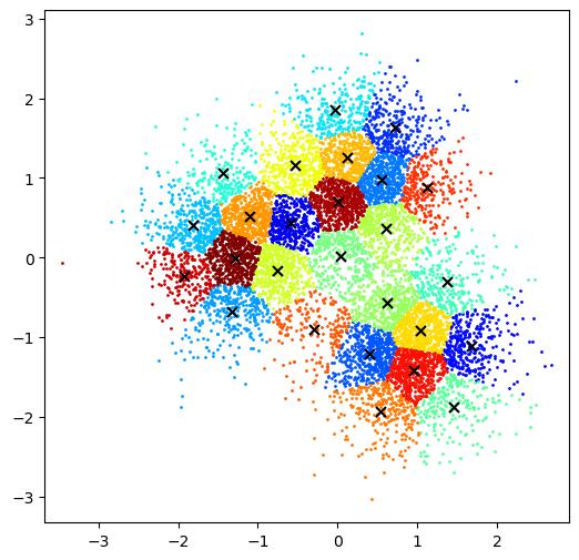
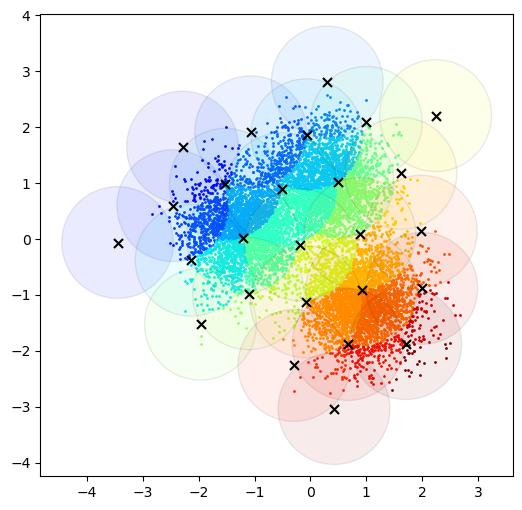
The visual difference between the two clustering methods is as shown in Figure 1. We can see that VQ (all achieved by k-means++ throughout the paper) assigns groups to form a Voronoi diagram while the GA partitions data of 10,000 points into groups that exist overlap. The partitions with overlap clusters (symbols) inherently model the natural semantic information of words in the real world, e.g., landlady and queen all refer to a woman. Therefore, we believe our joint symbolic representation has promising applications in time series with natural language processing techniques.
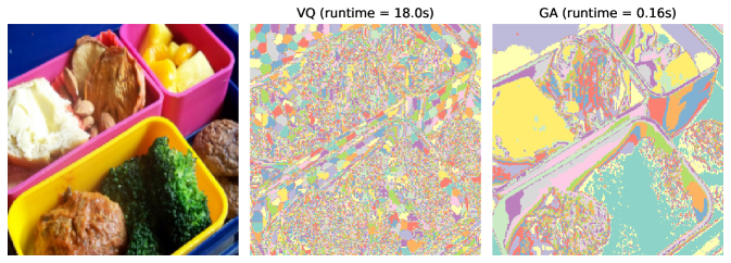
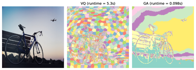
Both VQ and GA can perform clustering-based image segmentation tasks, where segmentation is completed by clustering the image’s pixels (each pixel represented as a 5-dimensional vector consisting of spatial coordinates and RGB color). Figure 2 shows the result of image segmentation of two images from the COCO dataset (Lin et al., 2014) by VQ and GA using the same number of clusters, respectively. GA performs clustering in image segmentation significantly faster than VQ, and we can also observe that GA performs well-separated segmentation which is closer to human perception compared to that of VQ which approaches a Voronoi-style segmentation.
4.1. Vector quantization
The k-means problems aim to find clusters within data in -dimensional space, so as to minimize the (5). However, solving this problem is NP-hard even is restricted to (Drineas et al., 2004; Dasgupta and Freund, 2008) or in the plane (Mahajan et al., 2012). Typically, the sub-optimal k-means problem can be solved by Lloyd’s algorithm (Lloyd, 1982b). In the implementation of ABBA software333https://github.com/nla-group/ABBA, the k-means algorithm is performed by scikit-learn library (Pedregosa et al., 2011) which runs a few times (this is controlled by the parameter n_init444The default to scikit-learn is 10 before the version 1.3.2.) of Lylod’s algorithm with seeding and pick up the best result. In the setting of this paper, we found setting n_init to 1 is good enough for the ABBA performance.
As already mentioned, Lloyd’s algorithm is a widely used method to solve the k-means problem, it starts with uniformly sampling centers from data, often referred to as seeding, and then each point is allocated to a cluster with the closest center, and the mean centers of clusters are recomputed again. The procedure keeps repeating until the iteration converges.
The seeding has a great impact on the final result. The improved algorithm is combined with optimal seeding “ weighting” introduced by (Arthur and Vassilvitskii, 2007), which can significantly improve Lloyd’s algorithm. Lloyd’s algorithm with weighting is called the “k-means++” algorithm. The k-means algorithm with “ weighting” shows -competitive with the optimal clustering.
ABBA digitization using this clustering method has been shown incredibly slow speed, though the reconstruction error meets the needs of most applications. It is very desired to design a faster clustering alternative while retaining the original reconstruction error to an ultimate degree. For this reason, we propose a sampling-based k-means clustering algorithm that can address the above concern. The idea is to perform k-means++ on a uniform sample of data where only percent of original data is used. The algorithm is as described in Algorithm 3. Section 6 will demonstrate its performance empirically.
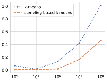
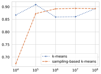
Figure 3 shows the simulation of k-means++ and sampling-based k-means (sampling of data) on Gaussian blobs data with 10 clusters, proceeding by increasing data sizes. The result is as illustrated in Figure 3. We can observe that sampling-based k-means runs in a fraction of the time compared to k-means++, while giving competitive performance in terms of adjusted mutual information (AMI).
4.2. Greedy aggregation
The greedy aggregation is introduced in (Chen and Güttel, 2022a), which proceeds first by sorting the data and performing greedy aggregation of data into groups. The sorting order naturally avoids unnecessary computations in aggregation by triggering an early stopping. The codebook set is constructed by the mean centers of the groups resulting from the aggregation as a suboptimal solution to the k-means problem. Though its accuracy is less significant than Lylod’s algorithm, it achieves a significant speedup and the SSE is upper bounded by for data points.
Sorting is essential to the success of aggregation in our context. Since sorting can determine the starting points selection and forming of groups, even helps to discard unnecessary distance computations. A bad sorting will result in inefficiency of aggregation and bad-performed SSE. For example, (Chen and Güttel, 2022b) proposes PCA sorting which ensures the pairwise distance between and is bounded by where is the second largest singular value of data matrix .
4.3. Parameter elimination
As aforementioned, digitization aims to partition described in (3) into clusters such that (5) is minimized. The tolerance-oriented digitization enables the natural relationship between compression tol and digitization . In this section, we discuss a novel way to eliminate the need of choosing a parameter for fABBA digitization. The Lemma 4.2 shows the reconstruction error still ensure the pin of start and end of time series.
Lemma 4.2 ((Elsworth and Güttel, 2020a)).
Mean-based clustering naturally leads to
Proof to Lemma 4.2 is as follows:
Also, we know that , hence, the reconstruction starts and ends at the same values as so is .
We assume variance of length and increment of pieces, denoted by and , are:
| (12) | ||||
Here we suppose the aggregation is performed on the length and increment values (1-dimensional data) of pieces simultaneously, which is referred to as hierarchical aggregation, and we denote the digitization tolerance for length and increment and , respectively. Obviously, we have
| (13) |
We assume , this yields
| (14) |
In the following, we will demonstrate that the Brownian bridge property as illustrated in (Elsworth and Güttel, 2020a) still holds in hierarchical aggregation for time series reconstruction. Though the length of each piece may not be consistent because of rounding error, we assume the length of the reconstructed time series is equal to the original length, i.e., (In practice, the assumption is true in most cases, but in some special cases, this does not hold true because of rounding). To simplify the modeling and facilitate the analysis, we consider only aggregating increment and assume each cluster of increment has the same mean length, i,e, . The local deviation of the increment and length value of on piece from the true increment and length of , which are given by
| (15) | ||||
respectively.
The global incremental errors, i.e., the accumulated incremental errors, according to (15), are given by:
| (16) |
Also, we must consider the error arisen from the rounding error of length. Similarly, the global length errors, i.e., the accumulated length errors, according to (12) and (13), can be calculated as:
| (17) | ||||
The global error of the reconstructed time series, denoted by , is caused by errors from reconstructed length and increment. Up to this point, the global error of the reconstructed time series is still difficult to determine since the estimated error caused by the length displacement is hard to get, so we consider an approximation:
| (18) |
According to (14) and Lemma 4.2, the is bounded by , and since they are consistent with the deviations from their respective cluster center. Also, as proved earlier. Therefore, referred to (Elsworth and Güttel, 2020a), we can model a random process of incremental errors , and its associated variance:
Following (Elsworth and Güttel, 2020a), is considered to stay standard deviations away from its zeros mean. That is, we consider a realization
| (19) |
The process of is modeled as a Brownian bridge following (Elsworth and Güttel, 2020a). Considering the interpolated quadratic function on the right-hand side is concave, based on the linear stitching procedure used in the reconstruction and by piecewise linear interpolation of the incremental errors from the course time grid to the fine time grid , it is natural to deduce that
| (20) |
Therefore, the squared Euclidean norm of this fine-grid “worst-case” realization is upper bounded by
It has previously been established that by (Elsworth and Güttel, 2020a), and based on this (4.3) is the worst-case realization of the Brownian bridge and thereby we have a probabilistic bound on the error incurred from digitization. By making , we can smartly choose
| (21) |
For simplicity we can set this hyperparameter controlling the tolerance of length to be the same as that of increment, i.e., . Therefore, the parameter of digitization is automatically determined by the compression tolerance, resulting in a non-parametric and error-bounded digitization procedure.
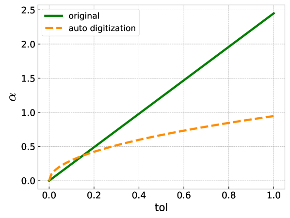
The procedure detailed above is referred to as auto digitization. On top of that, the method introduced in the Section 5 of (Elsworth and Güttel, 2020a) can also be used to approximate an error-bounded fABBA digitization and eliminate the need for tuning , however, this is not practical as it results in a linear relationship between tol and —the difference is as shown in Figure 4 which shows the method in (Elsworth and Güttel, 2020a) depicts a straight line (marked as green color). As a consequence, we can see our method (marked as orange color) as an improvement for choosing to some degree.
5. Joint symbolic approximation
After discussing the two ABBA methods, we introduce a joint symbolic aggregate approximation on how to perform fast ABBA symbolization on multiple time series while retaining the symbolic consistency. This joint approximation framework is also applicable to large-scale univariate time series and multivariate time series.
The ideal case of symbolization of multiple time series is that the symbolization should have consistent symbols used in each time series and as less distinct symbols used as possible. One intuitive idea is to fit one (or a given number of) time series and use the previous symbolic information to transform the rest of the data. However it does not consider the variety of characteristics in every single time series, this might result in serious information loss in some time series. Henceforth, we require an approach, i.e., joint symbolic approximation, that can symbolize the multiple time series simultaneously.
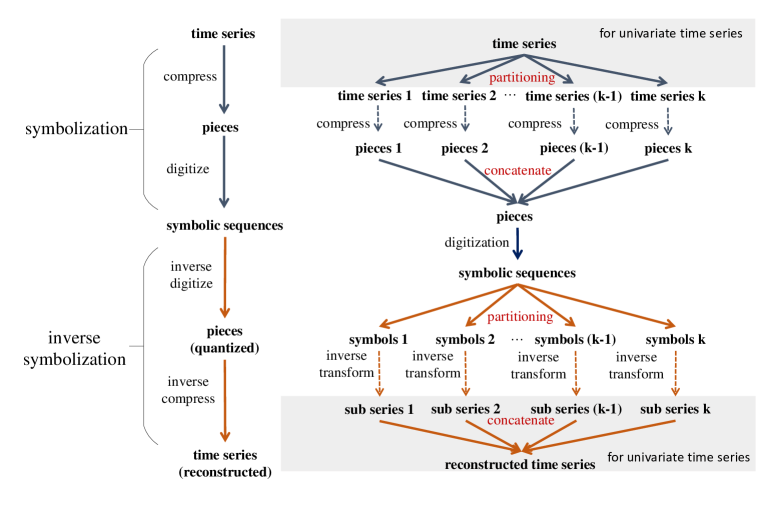
The essential idea of joint symbolic approximation is partitional compression. Let be a dataset of time series (If , simply partition the time series into multiple series). In contrast to the original compression, it proceeds by first computing the compression for each series. Then all outputs will be concatenated as an input to digitization which results in a single symbolic sequence. But for multiple time series, an additional step is required, i.e., divide the final symbolic sequence such that each partition corresponds to the symbolic representation of the original time series. The algorithm is as described in Algorithm 5. Since no dependencies occur between compression tasks, this allows for efficient parallel computing. The joint symbolic approximation as well as the parallel computing paradigm is as depicted in Figure 5 and the integral algorithm description is as illustrated in Algorithm 6. For the inverse symbolization, each time series can be reconstructed exactly from its first value and reconstructed pieces from inverse digitization.
The joint symbolic aggregate approximation essentially performs the same steps as the original ABBA method, the major difference is that the compression in ABBA is replaced with partitional compression. Since that, we refer to the method of joint symbolic aggregate approximation as JABBA for simplicity. The framework of joint symbolic aggregate approximation spawns two variants: (1) JABBA (VQ): performs partitional compression and digitization with k-means clustering; (2) JABBA (GA): performs partitional compression and digitization with greedy aggregation. Their performance will be evaluated in Section 6.
As aforementioned, the approach can be applied to datasets storing multiple time series such as UCR time series archive (Dau et al., 2019). With the availability of consistent symbols information, techniques of text mining and natural language processing are becoming promising in time series analysis.
6. Empirical Results
In this section, we focus on the experiments regarding runtime and reconstruction errors of symbolic representation. We conduct extensive experiments on the UEA Archive (Bagnall et al., 2018), which is a well-established dataset, and synthetic Gaussian noises for the multithreading test. We select the competing algorithms that provide publicly available software555Available at https://github.com/nla-group/ABBA and https://github.com/nla-group/fABBA., which is for simplicity and efficiency.
6.1. Multivariate time series test
The UEA Archive contains 30 multivariate time series datasets with a variety of dimensions and lengths. The datasets are very huge, therefore it is inefficient for the original ABBA and its variant fABBA to perform computations one at a time, so we select some datasets in the UEA Archive for the test, which are summarized in Table 2. Though impossible for ABBA and fABBA to symbolize time series in each dimension of multivariate time series with unified symbols, we still use them for benchmarking but without considering the symbolic consistency. In order to unify their compressed time series pieces as specified in (3), we use partitional compression for all four competing methods and reassign the subset of output corresponding to each multivariate time series dimension to ABBA and fABBA. We start with performing the partitional compression as described in Algorithm 5 with tol of 0.01, then for the two JABBA variants we perform their digitization all at once while for ABBA and fABBA we just perform their digitization on time series pieces for each dimension of the multivariate time series one at a time, and then record the runtime for their digitization, respectively.
It’s known that the more symbols are used the more accurate the reconstruction of the representation is. In order to use roughly the same number of symbols for each method as much as possible, we first perform JABBA (GA) digitization using (21) to confirm an value, and a total number of symbols used for the multivariate time series, denoted by , then we feed the number of symbols for JABBA (VQ) digitization (see Algorithm 3, we set to 0.5, same in the following). Then we feed the same value to fABBA digitization and use for ABBA where is the dimension of the multivariate time series. As a consequence, the number of symbols used will be unified for ABBA, JABBA (VQ), and JABBA (GA), but not guaranteed for fABBA since its digitization is tolerance-oriented.
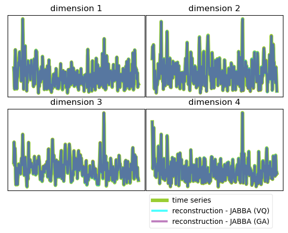
Table 3 showcases the average value of MSE, dynamic time warping (DTW), runtime for digitization, and the number of symbols used for each dataset. Information of compression tolerance tol used for each dataset is also given in Table 3. Accordingly, JABBA (GA) shows significant speedup over fABBA by order of magnitude though both use the same GA-based digitization. The speedup of JABBA (VQ) over ABBA is also remarkable while the reconstruction error of JABBA (VQ) is lower than ABBA in five out of the eight datasets though using sampling-based k-means is employed. Additionally, an example of reconstruction from symbolic representation for multivariate time series is presented in Figure 6, which only shows 4 out of 61 dimensions.
| Dataset | Size | Dimension | Length |
|---|---|---|---|
| AtrialFibrillation | 30 | 2 | 640 |
| BasicMotions | 80 | 6 | 100 |
| CharacterTrajectories | 2,858 | 3 | 182 |
| Epilepsy | 275 | 3 | 206 |
| Heartbeat | 409 | 61 | 405 |
| NATOPS | 360 | 24 | 51 |
| StandWalkJump | 27 | 4 | 2,500 |
| UWaveGestureLibrary | 440 | 3 | 315 |
| Dataset | Metric | ABBA | fABBA | JABBA (VQ) | JABBA (GA) |
| MSE | 6.7 | 69 | 9.7 | 63 | |
| AtrialFibrillation | DTW | 880 | 52,000 | 1,600 | 18,000 |
| () | Runtime | 160 | 15 | 23 | 2.6 |
| Symbols | 21 | 550 | 21 | 21 | |
| BasicMotions | MSE | 22 | 17 | 14 | 33 |
| DTW | 710 | 920 | 690 | 1,800 | |
| () | Runtime | 100 | 14 | 13 | 2.7 |
| Symbols | 17 | 460 | 18 | 18 | |
| CharacterTrajectories | MSE | 3.5 | 3.5 | 6.9 | 17 |
| DTW | 540 | 350 | 650 | 1,600 | |
| () | Runtime | 24 | 3.3 | 4.8 | 1.7 |
| Symbols | 3.1 | 47 | 3.5 | 3.5 | |
| Epilepsy | MSE | 20 | 50 | 15 | 86 |
| DTW | 1,700 | 20,000 | 1,400 | 13,000 | |
| () | Runtime | 83 | 12 | 31 | 2.2 |
| Symbols | 14 | 480 | 14 | 14 | |
| MSE | 5.2 | 0.0017 | 1.8 | 0.017 | |
| Heartbeat | DTW | 1,400 | 0.69 | 430 | 6.8 |
| () | Runtime | 17,000 | 1,500 | 3,500 | 110 |
| Symbols | 2,000 | 23,000 | 2,000 | 2,000 | |
| NATOPS | MSE | 38 | 18 | 9.1 | 28 |
| DTW | 1,700 | 270 | 150 | 430 | |
| () | Runtime | 110 | 28 | 100 | 2.5 |
| Symbols | 24 | 450 | 23 | 23 | |
| StandWalkJump | MSE | 2.2 | 8.7 | 3.7 | 5.7 |
| DTW | 550 | 5,100 | 730 | 1,200 | |
| () | Runtime | 900 | 60 | 55 | 11 |
| Symbols | 190 | 1,900 | 190 | 190 | |
| UWaveGestureLibrary | MSE | 3.1 | 2 | 3 | 8 |
| DTW | 350 | 180 | 340 | 1,100 | |
| () | Runtime | 37 | 3.8 | 5.7 | 1.9 |
| Symbols | 5.4 | 52 | 5.4 | 5.4 |
6.2. Multithreading simulation
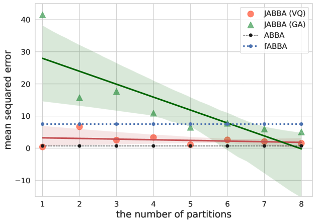
In this experiment, we will compare ABBA, fABBA, JABBA (GA), and JABBA (VQ) on synthetic Gaussian noise series in terms of runtime, and reconstruction accuracy with various number of time series partitions. The reconstruction accuracy is measured by MSE here.
We used Gaussian noises as the time series for benchmarking. The data generated for the test are of length 100,000 with zero mean and unit standard deviation. We first ran fABBA with and to compute the number of symbols it used. This simulation used 358 symbols accordingly. Second, we ran ABBA by feeding the same number of symbols fABBA used to , i.e., symbols. After that, we run the JABBA (VQ) and JABBA (GA) with varying partitions by the same tol and specifying a consistent hyperparameter setting for digitization, i.e., and , respectively. The number of threads scheduled for JABBA is set the same as the partition number. The result shows the compression rate computed for ABBA, fABBA, JABBA (GA), and JABBA (VQ) are , respectively.
The experimental result is as exhibited in Figure 7 and Figure 8. We mainly compare the methods with the same digitization technique. We can see that there is an obvious negative correlation between reconstruction error and the number of partitions, this can be explained by the increasing partition points that will be used for reconstruction. Figure 7 also shows that JABBA (VQ) which uses sampling-based k-means achieves similar performance against ABBA regarding MSE while performing speedup by orders of magnitude, a similar result applies to JABBA (GA) and fABBA.
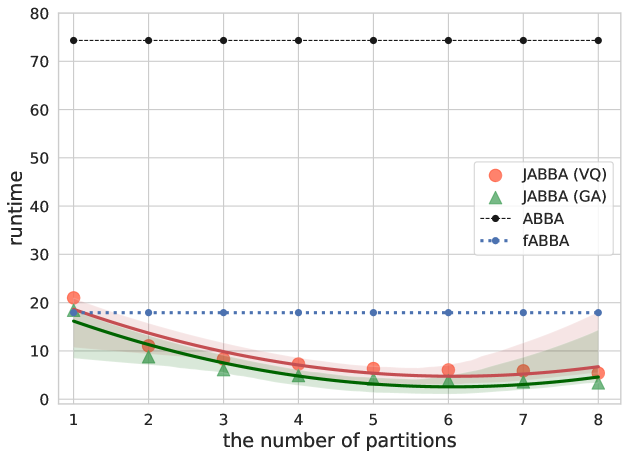
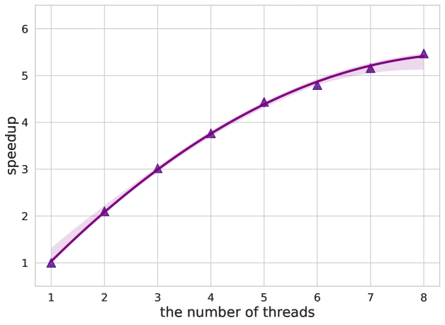
The parallel speedup processors is given by
where is referred to as the runtime of the processors. Without loss of generality, we only evaluate the speedup of Parallelism for JABBA (GA) as shown in Figure 9. We can see the speedup scale almost linearly with the number of threads . Since our algorithm is partially parallel in compression, which is hindered by the sequential part of the algorithm, that is, the digitization. This phenomenon can be naturally explained by Amdahl’s law which gives the theoretical speedup at a fixed workload where there are limits on the benefits one can derive from parallelizing a computation.
7. Summary and future work
The existing ABBA methods are incapable of handling the consistency of symbols for multiple time series and are inherently sequential, and it is not clear how to leverage the extra computational power such as multithreading processing. In this paper, we introduce a joint symbolic approximation method that improves the speed of ABBA symbolization and achieves symbolic consistency in each representation. The framework of joint symbolic approximation enables parallel computing for further speedup. Attributed to the symbolic consistency, a manipulation of natural language processing and text mining techniques is available in time series. The convergence analysis of our proposed sampling k-means method will be left as future work.
References
- (1)
- Agrawal et al. (1998) Rakesh Agrawal, Johannes Gehrke, Dimitrios Gunopulos, and Prabhakar Raghavan. 1998. Automatic subspace clustering of high dimensional data for data mining applications. Proceedings of the ACM SIGMOD International Conference on Management of Data 27 (1998), 94–105.
- Arthur and Vassilvitskii (2007) David Arthur and Sergei Vassilvitskii. 2007. k-means++: the advantages of careful seeding. In SODA ’07: Proceedings of the eighteenth annual ACM-SIAM symposium on Discrete algorithms. Society for Industrial and Applied Mathematics, 1027–1035.
- Bagnall et al. (2018) Anthony J. Bagnall, Hoang Anh Dau, Jason Lines, Michael Flynn, James Large, Aaron Bostrom, Paul Southam, and Eamonn J. Keogh. 2018. The UEA multivariate time series classification archive. CoRR (2018).
- Bountrogiannis et al. (2023) Konstantinos Bountrogiannis, George Tzagkarakis, and Panagiotis Tsakalides. 2023. Distribution Agnostic Symbolic Representations for Time Series Dimensionality Reduction and Online Anomaly Detection. IEEE Transactions on Knowledge and Data Engineering 35, 6 (2023), 5752–5766.
- Campello et al. (2013) Ricardo J. G. B. Campello, Davoud Moulavi, and Joerg Sander. 2013. Density-Based Clustering Based on Hierarchical Density Estimates. In Advances in Knowledge Discovery and Data Mining. Springer, 160–172.
- Chen and Güttel (2022a) Xinye Chen and Stefan Güttel. 2022a. An Efficient Aggregation Method for the Symbolic Representation of Temporal Data. ACM Transactions on Knowledge Discovery from Data (2022).
- Chen and Güttel (2022b) Xinye Chen and Stefan Güttel. 2022b. Fast and explainable clustering based on sorting. (2022), 25. arXiv:2202.01456
- Dasgupta and Freund (2008) Sanjoy Dasgupta and Yoav Freund. 2008. Random Projection Trees and Low Dimensional Manifolds. In Proceedings of the Fortieth Annual ACM Symposium on Theory of Computing (STOC ’08). ACM, 537–546.
- Dasgupta and Freund (2009) Sanjoy Dasgupta and Yoav Freund. 2009. Random Projection Trees for Vector Quantization. IEEE Transactions on Information Theory 55, 7 (2009), 3229–3242.
- Dau et al. (2019) Hoang Anh Dau, Anthony Bagnall, Kaveh Kamgar, Chin-Chia Michael Yeh, Yan Zhu, Shaghayegh Gharghabi, Chotirat Ann Ratanamahatana, and Eamonn Keogh. 2019. The UCR time series archive. IEEE/CAA Journal of Automatica Sinica 6, 6 (2019), 1293–1305.
- Drineas et al. (2004) P. Drineas, A. Frieze, R. Kannan, S. Vempala, and V. Vinay. 2004. Clustering large graphs via the singular value decomposition. Machine Learning 56, 1–3 (2004), 9–33.
- Elsworth and Güttel (2020a) Steven Elsworth and Stefan Güttel. 2020a. ABBA: adaptive Brownian bridge-based symbolic aggregation of time series. Data Mining and Knowledge Discovery 34 (2020), 1175–1200.
- Elsworth and Güttel (2020b) Steven Elsworth and Stefan Güttel. 2020b. Time series forecasting using LSTM networks: A symbolic approach. (2020), 12. arXiv:2003.05672
- Ester et al. (1996) Martin Ester, Hans-Peter Kriegel, Jörg Sander, and Xiaowei Xu. 1996. A Density-Based Algorithm for Discovering Clusters in Large Spatial Databases with Noise. In Proceedings of the Second International Conference on Knowledge Discovery and Data Mining (KDD’96). AAAI Press, 226–231.
- Gao and Lin (2019) Yifeng Gao and Jessica Lin. 2019. Discovering Subdimensional Motifs of Different Lengths in Large-Scale Multivariate Time Series. In IEEE International Conference on Data Mining. 220–229.
- Gray (1984) Robert Gray. 1984. Vector quantization. IEEE ASSP Magazine 1, 2 (1984), 4–29.
- Keogh et al. (2005) E. Keogh, J. Lin, and A. Fu. 2005. HOT SAX: efficiently finding the most unusual time series subsequence. In IEEE International Conference on Data Mining (ICDM’05). 1–8.
- Keogh et al. (2002) Eamonn Keogh, Stefano Lonardi, and Bill ’Yuan-chi’ Chiu. 2002. Finding Surprising Patterns in a Time Series Database in Linear Time and Space. In Proceedings of the Eighth ACM SIGKDD International Conference on Knowledge Discovery and Data Mining (KDD ’02). ACM, 550–556.
- Li and Lin (2017) Xiaosheng Li and Jessica Lin. 2017. Linear Time Complexity Time Series Classification with Bag-of-Pattern-Features. In IEEE International Conference on Data Mining. 277–286.
- Li et al. (2021) Xiaosheng Li, Jessica Lin, and Liang Zhao. 2021. Time Series Clustering in Linear Time Complexity. Data Mining and Knowledge Discovery 35, 6 (2021), 2369–2388.
- Li and Lin (2010) Yuan Li and Jessica Lin. 2010. Approximate Variable-Length Time Series Motif Discovery Using Grammar Inference. In Proceedings of the 10th International Workshop on Multimedia Data Mining (MDMKDD ’10). ACM, 9.
- Lin et al. (2003) Jessica Lin, Eamonn Keogh, Stefano Lonardi, and Bill Chiu. 2003. A symbolic representation of time series, with implications for streaming algorithms. In Proceedings of the 8th ACM SIGMOD Workshop on Research Issues in Data Mining and Knowledge Discovery. ACM, 2–11.
- Lin et al. (2007) Jessica Lin, Eamonn Keogh, Li Wei, and Stefano Lonardi. 2007. Experiencing SAX: a novel symbolic representation of time series. Data Mining and Knowledge Discovery 15, 2 (2007), 107–144.
- Lin et al. (2014) Tsung-Yi Lin, Michael Maire, Serge Belongie, James Hays, Pietro Perona, Deva Ramanan, Piotr Dollár, and C. Lawrence Zitnick. 2014. Microsoft COCO: Common Objects in Context. European Conference on Computer Vision (2014), 740–755.
- Lkhagva et al. (2006) B. Lkhagva, Yu Suzuki, and K. Kawagoe. 2006. New Time Series Data Representation ESAX for Financial Applications. In 22nd International Conference on Data Engineering Workshops (ICDEW’06). x115–x115. https://doi.org/10.1109/ICDEW.2006.99
- Lloyd (1982a) S. Lloyd. 1982a. Least squares quantization in PCM. IEEE Transactions on Information Theory 28, 2 (1982), 129–137.
- Lloyd (1982b) Stuart P. Lloyd. 1982b. Least squares quantization in PCM. Transactions on Information Theory 28 (1982), 129–137.
- Mahajan et al. (2012) Meena Mahajan, Prajakta Nimbhorkar, and Kasturi Varadarajan. 2012. The planar k-means problem is NP-hard. Theoretical Computer Science 442 (2012), 13–21. Special Issue on the Workshop on Algorithms and Computation (WALCOM 2009).
- Malinowski et al. (2013) Simon Malinowski, Thomas Guyet, René Quiniou, and Romain Tavenard. 2013. 1d-SAX: A Novel Symbolic Representation for Time Series. In Advances in Intelligent Data Analysis XII.
- Nguyen and Ifrim (2023) Thach Le Nguyen and Georgiana Ifrim. 2023. Fast Time Series Classification with Random Symbolic Subsequences. In Advanced Analytics and Learning on Temporal Data: 7th ECML PKDD Workshop, AALTD 2022, Grenoble, France, September 19–23, 2022, Revised Selected Papers. Springer, 50––65.
- Pedregosa et al. (2011) F. Pedregosa, G. Varoquaux, A. Gramfort, V. Michel, B. Thirion, O. Grisel, M. Blondel, P. Prettenhofer, R. Weiss, V. Dubourg, J. Vanderplas, A. Passos, D. Cournapeau, M. Brucher, M. Perrot, and E. Duchesnay. 2011. Scikit-learn: Machine Learning in Python. Journal of Machine Learning Research 12 (2011), 2825–2830.
- Ruta et al. (2019) N. Ruta, N. Sawada, K. McKeough, M. Behrisch, and J. Beyer. 2019. SAX Navigator: Time Series Exploration through Hierarchical Clustering. In 2019 IEEE Visualization Conference. IEEE, 236–240.
- Senin et al. (2015) Pavel Senin, Jessica Lin, Xing Wang, Tim Oates, Sunil Gandhi, Arnold P. Boedihardjo, Crystal Chen, and Susan Frankenstein. 2015. Time series anomaly discovery with grammar-based compression.. In 18th International Conference on Extending Database Technology. OpenProceedings.org, 481–492.
- Senin and Malinchik (2013) Pavel Senin and Sergey Malinchik. 2013. SAX-VSM: Interpretable Time Series Classification Using SAX and Vector Space Model. In IEEE International Conference on Data Mining. 1175–1180.
- Yu and Shi (2003) Stella X. Yu and Jianbo Shi. 2003. Multiclass spectral clustering. In Proceedings of the Ninth IEEE International Conference on Computer Vision, Vol. 2. IEEE, 313.
- Yu et al. (2023) Yuncong Yu, Tim Becker, Le Minh Trinh, and Michael Behrisch. 2023. SAXRegEx: Multivariate time series pattern search with symbolic representation, regular expression, and query expansion. Computers & Graphics 112 (2023), 13–21.
- Zhang et al. (2017) Shengdong Zhang, Soheil Bahrampour, Naveen Ramakrishnan, Lukas Schott, and Mohak Shah. 2017. Deep learning on symbolic representations for large-scale heterogeneous time-series event prediction. In 2017 IEEE International Conference on Acoustics, Speech and Signal Processing. 5970–5974.
- Zhang et al. (1996) Tian Zhang, Raghu Ramakrishnan, and Miron Livny. 1996. BIRCH: An efficient data clustering method for very large databases. In Proceedings of the ACM SIGMOD International Conference on Management of Data. ACM, 103–114.