Joint User Scheduling and Computing Resource Allocation Optimization in Asynchronous Mobile Edge Computing Networks
Abstract
In this paper, the problem of joint user scheduling and computing resource allocation in asynchronous mobile edge computing (MEC) networks is studied. In such networks, edge devices will offload their computational tasks to an MEC server, using the energy they harvest from this server. To get their tasks processed on time using the harvested energy, edge devices will strategically schedule their task offloading, and compete for the computational resource at the MEC server. Then, the MEC server will execute these tasks asynchronously based on the arrival of the tasks. This joint user scheduling, time and computation resource allocation problem is posed as an optimization framework whose goal is to find the optimal scheduling and allocation strategy that minimizes the energy consumption of these mobile computing tasks. To solve this mixed-integer non-linear programming problem, the general benders decomposition method is adopted which decomposes the original problem into a primal problem and a master problem. Specifically, the primal problem is related to computation resource and time slot allocation, of which the optimal closed-form solution is obtained. The master problem regarding discrete user scheduling variables is constructed by adding optimality cuts or feasibility cuts according to whether the primal problem is feasible, which is a standard mixed-integer linear programming problem and can be efficiently solved. By iteratively solving the primal problem and master problem, the optimal scheduling and resource allocation scheme is obtained. Simulation results demonstrate that the proposed asynchronous computing framework reduces energy consumption compared with conventional synchronous computing counterpart.
Index Terms:
Mobile edge computing, asynchronous computing, user scheduling, wireless power transfer.I Introduction
Mobile edge computing (MEC) provides powerful computing ability to edge devices [1, 2]. Numerous works have investigated MEC systems from the perspective of resource allocation. In [3], computing offloading and service caching are jointly optimized in MEC-enabled smart grid to minimize system cost. Work [4] proposed a reverse auction-based offloading and resource allocation scheme in MEC. With the aid of machine learning, a multi-agent deep deterministic policy gradient (MADDPG) algorithm is designed to maximize energy efficiency in [5]. However, deploying computing resources at edge servers of a wireless network faces several challenges. First, due to limited energy of edge servers, they may not be able to provide sufficient computation resource according to devices’ requirements [6, 7]. Second, executing all offloading tasks synchronously requires edge servers to wait the arrival of the task with maximum transmission delay which may not be efficient. Meanwhile, task scheduling sequence is nonnegligible in synchronous task offloading, which will also impact the network loads and task completion [8].
To address the first challenge, wireless power transfer (WPT) technology that exploits energy carried by radio frequency (RF) signals emerges [9]. Instead of using solar and wind sources, ambient RF signals can be a viable new source for energy scavenging. Harvesting energy from the environment provides perpetual energy supplies to wireless devices for tasks offloading [10]. Thus, WPT has been regarded as a promising paradigm for MEC scenarios. Combining WPT with MEC, the authors in [11] proposed a multi-user wireless-powered MEC framework aiming at minimizing the total energy consumption under latency constraints. In [12], considering binary computation offloading, the weighted sum computation rate of all wireless devices was maximized by optimizing computation mode selection and transmission time allocation. The work in [13] proposed a multiple intelligent reflecting surfaces (IRSs) assisted wireless powered MEC system, where the IRSs are deployed to assist both the downlink WPT from the access point (AP) to the wireless devices and the uplink computation offloading. However, the above works [14, 15, 16, 17, 11, 12, 13] assumed that all computational tasks offloaded by users will arrive at the server at the same time and then the server starts to process all tasks simultaneously, which is not efficient and even impractical due to users’ dynamic computational task processing requests [18].
Currently, only a few existing works [18, 19, 20, 21, 22, 23] optimized MEC networks under dynamic computation requests. The work in [18] designed a Whittle index based offloading algorithm to maximize the long-term reward for asynchronous MEC networks where computational tasks arrive randomly. In [19], the authors studied the co-channel interference caused by asynchronous task uploading in NOMA MEC systems. The work in [20] investigated the energy efficient asynchronous task offloading for a MEC system where computational tasks with various latency requirements arrive at different time slots. Task scheduling problem for MEC systems with task interruptions and insertions was studied in [21]. However, the above works [18, 19, 20, 21] that focused on the asynchronous task offloading neglected how the asynchronous task arrival affects the computation at the MEC server. The authors in [22] used a sequential computation method to solve the energy consumption minimization problem under asynchronous task arrivals. The work in [23] designed a computation strategy that only allows a task to be executed after the completion of the previous tasks. Yet, works in [22] and [23] are still constrained by their limited usage of the server computation capacity, and cannot act as resource efficient asynchronous task offloading solutions.
The sequential computation strategy [24] has shown to have the potential to improve the computation resource efficiency and task execution punctuality in an asynchronous MEC network. However, since the computation resource allocation at the server depends on the arrival of the offloaded tasks, the sequential scheduling of the tasks will inevitably affect system performance, which is a fact that has been wildly ignored [22, 25, 26].
The main contribution of this paper is a novel asynchronous MEC framework that jointly schedules tasks and allocates computation resource with optimized system energy efficiency. In brief, our key contributions include:
-
•
We develop a novel framework to manage computation resource for the sequential computation in asynchronous MEC networks. In particular, we consider a MEC network in which the edge devices sequentially harvest energy for transmission, offload their computational tasks to a MEC server, and then compete for computation source at the server to get their tasks accomplished. To achieve the high energy efficient task execution, a policy needs to be designed for determining the optimal task scheduling sequence, time and computational resource allocation. We pose this joint scheduling and resource allocation problem in an optimization framework and seek to find the strategy which minimizes the energy consumption of the tasks.
-
•
Then, a general benders decomposition (GBD) based algorithm is proposed to solve the formulated mixed-integer non-linear programming (MINLP) problem which is decomposed into a primal problem that allocates computation resource and time, and a master problem that schedules user tasks. By iteratively solving the primal problem and master problem, the optimal scheduling and resource allocation scheme is obtained.
-
•
To show the effectiveness of the proposed algorithm, we prove that the optimal energy efficient scheduling and resource allocation scheme also optimizes the task punctuality. Our analytical results also show that the optimal allocation scheme for a given offloading task follows a specific pattern: the computation frequency allocated to each task remains constant initially, then gradually decreases before eventually reaching zero. Notably, all tasks experience a simultaneous decrease, the time of which is given in a closed form, in terms of their required central processing unit (CPU) cycles. Leveraging these identified properties, we introduce a computation resource allocation algorithm that offers a low-complexity solution.
Simulation results demonstrate that the proposed asynchronous computing framework reduces energy consumption compared with conventional synchronous computing counterpart. Moreover, computational complexity of the proposed computation resource allocation algorithm is reduced by times compared with conventional interior point method.
The rest of this paper is structured as follows. Section II elaborates system model and problem formulation. In Section III, we investigate the properties of asynchronous frequency allocation with given time allocation and user scheduling. The joint optimization of user scheduling, time allocation, and computation resource allocation is rendered in Section IV. Simulation results are presented in Section V. Finally, Section VI draws the conclusions.
II System Model and Problem Formulation
Consider a MEC network consisting of one MEC server, and a set of energy harvesting enabled edge devices. Within this network, each device needs to execute an bits computational task, and will offload its computational task to the MEC server. As shown in Fig. 1, the devices need to first harvest energy from the server to enable such offloading. Then, using the time division multi-access (TDMA) technique, the devices need to schedule their offloading toward the MEC server. In other words, the computational tasks offloaded by devices will arrive at the MEC server asynchronously. To this end, the MEC server will process each device’s computational task in an asynchronous manner. In particular, the server will process devices’ computational tasks according to the time that it receives each of these computational tasks.
The server and edge devices must complete their computational tasks within a time period which is divided into time slots. The duration of each time slot is represented by , with . Each device uses one time slot to offload its computational task. Let be the index to indicate whether device offloads its task to the server at time slot . In particular, if device uses time slot to offload its computational task, we have ; otherwise, . Since each device uses only one time slot and each time slot can only be allocated to one device, we have , and . Meanwhile, when , device will harvest energy from time slot to . Once task arrives at the MEC server, i.e., at time slot slot , the server will process this computational task.
The task computation process of the server and a device jointly completing a computational task consists of three stages: 1) energy harvesting, 2) task offloading, and 3) remote computing. Next, we first introduce the process of the energy harvesting, task offloading, and remote computing stages. Then, the problem formulation is given.
II-A Energy Harvesting Model
The path loss model is given by , where represents antenna gain, denotes the speed of light, is the carrier frequency, denotes the path-loss factor, and represents the distance between device and the server [27]. The instant channel gain between device and server denoted by , follows an i.i.d. Rician distribution with line-of-sight (LoS) link gain equal to , where is Rician factor. If device offloads its task at time slot (i.e., ), the harvested energy of device is , where is the energy harvesting efficiency of each device, which is assumed to be equal for all devices [28]. denotes the transmit power of the server. Since each device has only a single time slot for task offloading (i.e., there exists only one such that for a certain device ), the energy harvested by device can be reformulated by .
II-B Tasks Offloading Model
Based on the monomial offloading power model [20, 29], the transmit power of device at its offloading time slot is
| (1) |
where is the transmission rate, is the energy coefficient related to the bandwidth and the noise power, and the order is the monomial order associated with coding scheme. Since the transmit power of devices comes from harvested energy, we have .
II-C Computing Model
The MEC server is equipped with multiple CPUs such that the computational tasks offloaded from different devices can be executed in parallel [30]. Let be the computation intensity of task in terms of CPU cycles per bit. As shown in Fig. 2, to sufficiently utilize asynchronous computing, the computation resource of the server will be reallocated to the computational tasks offloaded from devices at each time slot from to . Intuitively, the first uploading task can occupy the whole computation capacity of the server before the second offloading task arrives, while all the tasks compete for computation resource at time slot . At an arbitrary time slot , , is set to be the computation resource allocated to the task that arrives at the server at time slot . Given these definitions, we have , where represents the maximum computation capacity of the MEC server. To complete the task computation for each device , we have , where represents the computation cycles of device . Besides, the energy consumption of the MEC server for all tasks computation can be formulated by , where denotes the energy coefficient of the MEC server.
II-D Problem Formulation
Our goal is to minimize the MEC server’s energy consumption of completing the tasks offloaded by all devices, which is formulated as an optimization problem as
| (2) | ||||
| s.t. | (2a) | |||
| (2b) | ||||
| (2c) | ||||
| (2d) | ||||
| (2e) | ||||
| (2f) | ||||
| (2g) | ||||
where , , and . In (2), (2a) is energy consumption causality constraint; (2b) represents a computational resource allocation constraint; (2c) ensures the completion of task computing; (2d) implies that the execution time of all devices should be less than ; (2e)-(2g) are user scheduling constraints. Since the discrete user scheduling variables and continuous resource allocation variables , are highly coupled, problem (2) is a standard MINLP problem which is difficult to solve. To handle this issue, we first analyze the optimal computation resource allocation with given user scheduling and time allocation in Section III, based on which an efficient low-complexity computation frequency optimization algorithm is proposed. Finally, in Section IV, we propose a GBD-based algorithm to jointly optimize user scheduling and resource allocation so as to solve problem (2). 111 For multi-server edge computing systems, new indicator variables can be introduced to denote the association between tasks and servers. Then the energy minimization problem can be formulated as a MINLP problem containing two kinds of binary optimization variables for task-server association and scheduling sequence, respectively. Despite being more complex, the problem can be solved efficiently using conventional MINLP methods such as convex relaxation and branch-and-bound, or latest approach using machine learning (see e.g., [27]). It is worth noting that with given task-server association, the proposed algorithm in this work is still applicable to scheduling and resource allocation optimization for each server. The detailed transmission protocol and algorithm procedure are left for future works.
III Analysis and Algorithm of the Optimal Computation Resource Allocation
In this section, we first analyze the properties of the optimal computation resource allocation, and then a low-complexity computation resource allocation algorithm is accordingly proposed. For ease of notation, we use to represent the computation cycles to complete the task that arrives at the server with order . With given time slot allocation vector and user scheduling matrix , problem (2) is simplified as follows:
| (3) | ||||
| (3a) | ||||
| (3b) | ||||
| (3c) | ||||
Before solving problem (3), we provide the feasibility condition as follows.
Proposition 1.
Problem (3) is feasible if and only if .
Proof.
Please refer to Appendix A. ∎
Denote , , and as the non-negative Lagrangian multipliers associated with the maximum frequency constraints (3a), task computation completion constraints (3b) and non-negative frequency constraints (3c), respectively. The optimal computation resource allocation is given by the following proposition.
Proposition 2.
Given the optimal , , the optimal solution of problem (3) is given by
| (4) |
Proof.
Since (4) can be effectively obtained by solving Karush-Kuhn-Tucker (KKT) and Slater conditions, the proofs is omitted here. ∎
According to Propostion 2, we can use the sub-gradient method to obtain the optimal and so as to acquire the optimal computation resource allocation. To further reduce the computational complexity and provide some design insights, the properties of the optimal solution of problem (3) are summarized in the following theorem.
Theorem 3.
Denote . The optimal computation resource has the following properties:
-
1)
The optimal solution of problem (3) satisfies , where is referred as “transition point”.
-
2)
The optimal satisfies .
-
3)
The transition point is if and only if .
According to property 1) in Theorem 3, the optimal frequency allocation scheme for a certain offloading task always follows a specific pattern: the frequency allocated to each device remains constant initially, then gradually decreases and eventually reaches zero. This property motivates us to deduce the condition . The property 2) in Theorem 3 implies that the computation resource of the server is redundant at time slots from to , while the maximum computation resource is utilized at slots from to .
According to property 1) in Theorem 3, unless , there always exists a special time slot we called “transition point” such that . The transition point indicates the number of time slots that the computation resource remains the same. The computation resource decreases for all tasks at the transition point. The method to find out the transition point when it exists is given by property 3) in Theorem 3.
Property 3) in Theorem 3 also shows that the transition point is impacted by the computation ability of the server. We can directly determine the transition point utilizing property 3) in Theorem 3 without the need of solving problem (3). After determining the transition point, we have according to property 2) in Theorem 3.
Fig. 3 depicts an illustration of properties in the optimal computation resource allocation. As can be seen, before the transition point , the optimal and keeps unchanged as . Based on Theorem 3, a low-complexity algorithm is proposed in Algorithm 1. First, we check the feasibility of problem (3) according to Proposition 1. Then, we determine the transition point based on property 3) in Theorem 3. If there is no transition points, which means that the computation resource of server is abundant, we can directly obtain the optimal solution for ; otherwise, we obtain the transition point and have for . Hence, we only need to find out the optimal and . Note that with given , we can obtain the optimal by solving the following equalities
| (5) |
since the maximum frequency is utilized at time slots from to . Since decreases with respect to , the bisection method is adopted. It should be noticed that achieves the maximum value of when and the minimum value of when . Therefore, the upper bound of is set as . For the lower bound, we set according to property 2) in Theorem 3. After obtaining for , is updated by a sub-gradient method [31], where is the dynamically chosen step-size. Through repeating Steps 5 to 13 until the objective of (3) converges, we can obtain the optimal for and for .
The complexity of Algorithm 1 is , where denotes the accuracy of the bisection method and is the accuracy of the objective of problem (3). Compared with the complexity of by the interior point method, the complexity of the proposed algorithm is significantly reduced. Moreover, when is large, the complexity can be further reduced since more numbers of are zeros.
IV Joint User Scheduling and Resource Allocation Algorithm
In this section, we employ the GBD method to solve problem (2). The core idea of GBD method is decomposing the original MINLP problem into a primal problem related to continuous variables and a master problem associated with integer variables, which are iteratively solved222Interested readers may refer to [29, 32, 33, 34] for details. . Specifically, for problem (2), the primal problem is a joint communication and computation resource optimization problem with fixed user scheduling. The master problem optimizes user scheduling by utilizing the optimal solutions and dual variables of the primal problem. Next, we describe the detailed procedures.
IV-A Primal Problem
With given user scheduling , problem (2) is reduced to the following optimization problem:
| (6) | ||||
| (6a) | ||||
| (6b) | ||||
| (6c) | ||||
where denotes the index of the -th offloading device, i.e., we have if . Since the user scheduling scheme is known, the value of can be deduced and substituted into problem (2). Since problem (6) is non-convex due to the constraints (6a), (6b) and the objective, we introduce to represent computation amounts of the -th offloading task at time slot . Hence, problem (6) is equivalent to
| (7) | ||||
| (7a) | ||||
| (7b) | ||||
| (7c) | ||||
where is the collections of . It can be proved that problem (7) is convex utilizing the tricks of perspective function [35]. To further provide useful insights and reduce computation complexity, we utilize the block coordinate decent (BCD) method to iteratively optimize time allocation and computation resource. Since the low-complexity computation resource allocation algorithm with given time allocation has been provided in Algorithm 1, next we propose time allocation algorithm with fixed computation resource allocation.
The Lagrangian function of problem (7) with respect to is given by
| (8) |
where , and are dual variables related to constraints (6a), (7a) and (2d), respectively. Taking the derivative with respect to , we have
| (9) | ||||
| (10) | ||||
| (11) | ||||
| (12) | ||||
| (13) |
Through solving above equations, the optimal is obtained in the following proposition.
Proposition 4.
The optimal is given by
| (14) | |||
| (15) | |||
| (16) | |||
| (17) |
and is the null point of , where , .
Through iteratively optimizing time allocation and computation resource allocation, we can obtain the optimal solution of primal problem (7). However, if problem (7) is infeasible, we formulate the corresponding -minimization problem as follows:
| (18) | ||||
| (18a) | ||||
| (18b) | ||||
| (18c) | ||||
Since problem (18) is convex and always feasible, we can use the interior point method to obtain the optimal solution and corresponding dual variables.
Furthermore, we can observe that the solution of primal problem always provides a performance upper bound for problem (2) since user scheduling is fixed. Then the upper bound is updated as , where denotes the objective value of primal problem (6). As can be seen, the upper bound is always non-increasing as iteration proceeds. Subsequently, we construct master problem using the solutions and dual variables of primal problem (7) and feasibility problem (18).
IV-B Master Problem
At each iteration, optimality cut or feasibility cut are added to master problem depending on whether the primal problem is feasible. Denote and as the set of iteration indexes indicating the primal problem is feasible and infeasible, respectively. Specifically, the optimality cut for each of feasible iterations is defined as
| (19) |
where and represent the dual variables related to primal problem at the -th iteration, and denote the solution of primal problem at the -th iteration. The terms irrelavant to are omitted based on complementary slackness theorem [31]. Similarly, the feasibility cut for each of infeasible iterations is defined as
| (20) |
where and represent the dual variables related to feasibility problem at the -th iteration, and denote the solution of feasibility problem at the -th iteration. Therefore, master problem is formulated as
| (21) | ||||
| (21a) | ||||
| (21b) | ||||
| (21c) | ||||
In particular, (21a) and (21b) denote the set of hyperplanes spanned by the optimality cut and feasibility cut from the first to the -th iteration, respectively. The two different types of cuts are exploited to reduce the search region for the global optimal solution [36]. Master problem (21) is a standard mixed-integer linear programming (MILP) problem, which can be solved by numerical solvers such as Gurobi[37] and Mosek[38]. Since master problem is the relaxing problem of MINLP problem (2), solving master problem provides a performance lower bound for problem (2). The lower bound is given by . Since at each iteration, an additional cut (optimality cut or feasibility cut) is added to master problem which narrows the feasible zone, the lower bound is always non-decreasing. As a consequence, the performance upper bound obtained by primal problem and the performance lower bound obtained by the master problem are non-increasing and non-decreasing w.r.t. the iteration index, respectively. As a result, the performance upper bound and the performance lower bound go to converge [29]. Therefore, through iteratively solving primal problem and master problem, we can obtain the optimal solution when the upper bound and lower bound are sufficiently close [33, 36]. The detailed algorithm is summarized in Algorithm 2.
IV-C Complexity Analysis
The complexity of solving problem (2) by Algorithm 2 lies in solving the primal problem, feasibility problem, and master problem at each iteration. For primal problem, where we iteratively update time allocation variables and frequency variables. The frequency optimization method is given in Algorithm 1, whose complexity is as analyzed in Section III. The time allocation optimization is according to Proposition 4, whose complexity is estimated as . Therefore, the total complexity of solving primal problem is , where denotes the iteration number in the primal problems. For the feasibility problem, the complexity is given by by the interior point method. For the master problem, the computational complexity is by the Branch and Bound (BnB) method [39].
V Simulations
In this section, we perform simulations to validate the proposed scheme and algorithm. There are devices around the server. The task size and computation intensity obey uniform distribution on Kbits and cycles/bit, respectively. The transmit power of BS is W. The energy coefficient of the MEC server and energy conversion factor of devices are set as and . We set the energy constant of transmission . Furthermore, the maximum computation resource is GHz and the allowable delay is second. In channel model, we set antenna gain , carrier frequency MHz, path-loss factor , speed of light m/s, and the Rician factor is . The following benchmarking schemes are provided:
-
•
JSORA[26]: The joint sensing-and-offloading resource allocation algorithm, where the allocated frequency for each device keeps unchanged during its computation duration, i.e., .
- •
- •
-
•
Exhaustive search: We randomly choose multiple initial points for Algorithm 2 and select the smallest result as output. The results of exhaustive search method can be regarded as global optimal solutions.
Besides, all accuracies used in the simulations are set as for fairness.
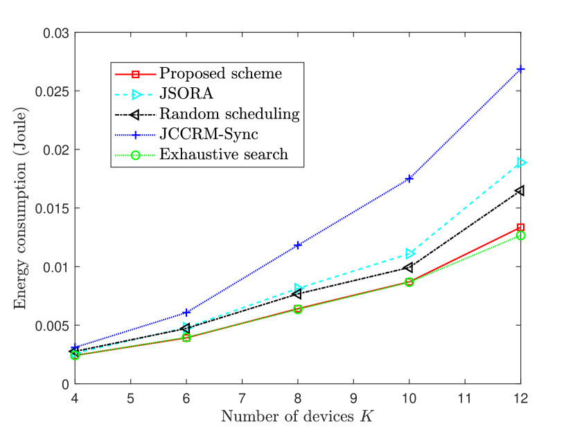
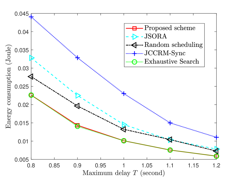
Fig. 5 demonstrates the energy consumption performance comparisons between different schemes under different numbers of devices. We can observe that the energy consumption of the proposed scheme as well as benchmark schemes increases with the number of devices getting large. This is because that devices have to compete for fixed communication and computation resource. As the number of devices increases, the average transmission time and computation time of each device get small, thus average computation resource becomes large. Therefore, larger energy consumption of server is required in order to finish devices’ tasks within the required delay. Moreover, as can be seen in Fig. 5, the gap between the proposed algorithm and exhaustive search scheme is small. This indicates that the proposed algorithm achieves close-to-optimal solutions. Compared with JSORA scheme, random scheduling scheme and JCCRM-Sync scheme, the proposed scheme achieves , , energy reductions, respectively. This can be explained by that the proposed algorithm can take full advantage of the flexibility of asynchronous computing and user scheduling. Particularly, compared with the proposed scheme, JCCRM-Sync scheme wastes the idle computation resource from time slots to . Similarly, JSORA scheme can not make full use of computation resource from time slots to . Hence, its performance is better than JCCRM-Sync but worse than the proposed scheme. Additionally, random scheduling, as most of the existing literature does, can not utilize the heterogeneity of tasks size and computation intensity well in MEC networks.
In Fig. 5, we depict the energy consumption curves of different schemes versus the maximum allowable delay. As can be seen, the energy consumption of all schemes decreases as the maximum delay becomes large. This is because as delay gets large, the server has more time to finish tasks. Thus, the fewer computation resource is allowable. Hence, energy consumption can be reduced. From Fig. 5, it can be verified that the proposed algorithm outperforms benchmarking schemes in terms of energy consumption in the considered region of delay, especially in resource-scarce scenarios. This phenomenon can be observed in Fig. 5 and Fig. 5 that the difference in energy consumption between the proposed algorithm and benchmark schemes gets small when resource is abundant. This is because the flaws of benchmark schemes compared with the proposed algorithm can be appropriately compensated by utilizing additional sources. Furthermore, it should be noticed that JSORA scheme is equivalent to the proposed scheme when computation resource is abundant according to Theorem 3.
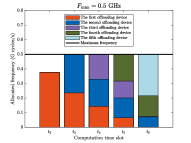
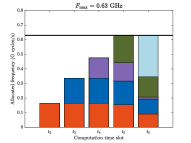
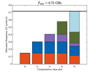
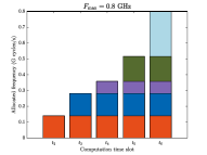
Fig. 6 illustrates a specific case of the allocated frequency of each device at each computation slot under different maximum computation frequencies when . It can be seen that as the maximum frequency becomes large, the transition point is gradually postponed, and finally no transition point exists when computation resource is sufficiently large which is in accordance with Theorem 3. Specifically, for each subfigure, we can find that before the transition point, the allocated frequency for each device being computed remains unchanged and the maximum frequency constraints do not work. From the transition point to the end, the allocated frequency for each device becomes small and the maximum frequency of the server is used. This verifies Theorem 3.
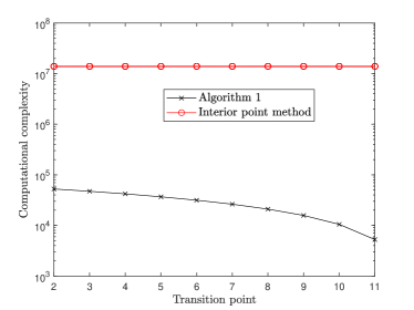
Fig. 7 depicts the computational complexity comparisons between the proposed Algorithm 1 and the interior point method under different transition points. As can be seen, the computational complexity of Algorithm 1 is significantly reduced compared with the interior point method, by more than times on average. As the transition point becomes larger, the complexity further decreases. For example, when the transition point , the complexity of Algorithm 1 is reduced by times. This is because the proposed computation resource allocation algorithm fully utilizes the properties in Theorem 3 to reduce algorithm complexity, especially when the computation resource of the server is abundant.
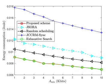
To test the compatibility of the proposed algorithm under different task scale differences, the energy consumption versus minimum task size is shown in Fig. 8, where task size obeys uniform distribution on with fixed mean value Kbits. With a large , the task scale difference is small. In Fig. 8, the proposed scheme and exhaustive search scheme achieve nearly the same performance, and outperform other schemes. One can observe that the energy consumption increases as task scale difference gets large. This can be explained by that the resources have to be tilted towards the devices with large task sizes, thus resulting in more energy consumption.
VI Conclusion
In this paper, we have investigated a joint user scheduling and resource optimization framework for MEC networks with asynchronous computing. An optimization problem of joint user scheduling, communication and computation resource management has been solved aiming to minimize the energy consumption of server under the delay constraint. Simulations verified that the proposed algorithm yields significant performance gains compared with benchmark schemes. This work establishes a new principle of asynchronous computing and verifies the superiority over its synchronous counterpart. For future works, we will generalize the proposed asynchronous computing framework to heterogeneous task deadlines scenarios so as to further activate its potential. As another direction, the extension to online algorithm design and accommodate new coming devices deserve further investigation.
Appendix A Proof of Proposition 1
The feasibility problem of (3) can be constructed as
| (A.1) | ||||
| (A.1a) | ||||
| (A.1b) | ||||
If the optimal objective of problem (A.1) is less than or equal to , problem (3) is feasible; otherwise, it is infeasible. Subsequently, we analyze the optimal solution of problem (A.1). First, when , i.e., there exists only one task, the optimal objective of problem (A.1) is . When , we consider two cases: 1) If , this indicates that the optimal scheme is computing task after task is finished. Therefore, the optimal solution is and . Hence, the optimal objective is . 2) If , this implies that part of task can be processed in parallel with task . Hence, the optimal solution is given by . Since , the optimal objective is . In conclusion, when , the optimal objective is . Similarly, by recursion, we can deduce that when there exist TD, the optimal solution is . That completes the proof.
Appendix B Proof of Property 1) in Theorem 3
Before that, we give the following two corollaries to facilitate the proof.
Corollary 5.
[Row property] The optimal computation resource of each task is non-increasing during its computation period, i.e., .
Proof.
Please refer to Appendix E. ∎
Corollary 6.
[Column property] Denote the sum computation cycles of the -th offloading device in time slots and by for and . If holds for all , the optimal frequency shifts are either all zeros or all positive, i.e., have the coincident zero or positive characteristics.
Proof.
Please refer to Appendix F. ∎
First, applying the KKT conditions gives
| (B.1) | |||
| (B.2) | |||
| (B.3) | |||
| (B.4) | |||
| (B.5) |
Based on (B.1), we obtain that
| (B.6) |
In case of , we have according to (B.4). Furthermore, is derived from (B.6). According to Corollary 5, the optimal solution satisfies . Thus, we have . Assume that there exists a certain such that . We have . If , i.e., and , we should have according to (B.2). Furthermore, due to , the computation cycles . According to Corollary 6, we have . Hence, it can be derived that which contradicts that is positive. Therefore, we have , i.e., . Since and , we can further obtain that . This indicates that if there exists a certain such that , we have .
Additionally, if there exists a certain such that , we can deduce that since .
Combing the above two cases, we complete the proof.
Appendix C Proof of Property 2) in Theorem 3
Appendix D Proof of Property 3) in Theorem 3
We first prove the “only if” part. According to property 1) in Theorem 3, if is the transition point, we have and . Since , we can obtain that . Thus, we have , i.e., .
Similarly, if is the transition point, we have . Since , we should have .
For the “if” part, if , we can deduce that . Moreover, since , we have , i.e., . Since , we can obtain that . Therefore, to let hold, we should have . Further, it can be deduced that .
Additionally, since , we can deduce that . Thus, we have , which indicates that the computation resource is abundant from to . Therefore, we can deduce that . Assume that is the transition point. We have . Since , is infeasible, which breaks the assumption. Therefore, we can conclude that is the transition point.
Combining the proofs of “if” and “only if” part, we complete the proof.
Appendix E Proof of Corollary 5
To find out the optimal computation resource allocation scheme, we first investigate the property of the most energy-efficient scheme without the maximum frequency restriction in Lemma 7, whose proof is provided in Appendix G.
Lemma 7.
Regardless of , and with given computation cycles in time slots and , scheme consumes the least energy among all the solutions satisfying .
For Corollary 5, we first prove that with given computation cycle and . Denote the sum computation cycles in and of the first offloading device as . Through relaxing the maximum computation resource constraint, the energy consumption is the least when according to Lemma 7. Since constraint (3a) should be satisfied, we have
| (E.1) |
We consider the following two cases; otherwise, and have no feasible solution with the given .
Case 1: . In this case, we can deduce that satisfies (E.1). Since is the most energy efficient solution, the optimal solution in this case is .
Case 2: . Obviously, is infeasible in this case. We then prove that is also impossible. Since , increases as decreases. If , we can deduce that . Therefore, we have which violates the maximum frequency constraint. As a consequence, the optimal solution is . According to Lemma 7, the energy consumption increases with in the considered region . Therefore, in order to achieve the fewest energy consumption, we should let as small as possible. Hence, we can obtain that and . The corresponding optimal .
Summarizing the above two cases, we can obtain that . Subsequently, we prove that in and , we always have for all .
Denote the sum computation cycles of the -th offloading device in time slots and by , i.e.,
| (E.2) |
According to Lemma 7, when for all , the minimum energy consumption of the -th offloading device can be achieved, thus the total energy consumption is minimum. Moreover, the following constraints should be satisfied:
| (E.3) |
We consider two cases.
Case 1: . In this case, we can deduce that for all satisfies (E.3). Thus, the optimal solution in this case is for all .
Case 2: . Obviously, is infeasible in this case. We then prove that by contradiction. By summing all the equalities in (E.2), we have . Thus, is negatively correlated with . If , it can be inferred that . We can further have which violates constraint (E.3). Similarly, if , we can obtain that . Hence, we have which breaks constraint (E.3). As a consequence, the optimal solution in this case satisfies .
Next, we prove that for all . With given and , we denote the energy consumption of the -th offloading device by , where . According to (G), is expressed by
| (E.4) |
which decreases when while increases when .
Furthermore, since , we have
| (E.5) |
According to (E), we have . Next, we utilize contradiction to prove that for all . Assume in the optimal solution there exists a certain . We can suitably decrease other positive and increase the negative to zero while keeping unchanged. In this case, the total energy consumption is effectively reduced, which contradicts the optimality. That completes the proof of , i.e., for all .
In summary, since we have proven and for and , we can deduce Corollary 5.
Appendix F Proof of Corollary 6
In case of , the optimal are all zeros according to Corollary 5. Therefore, we only need to justify the case of . In this case, we first prove that the optimal . Assume that the optimal . We can suitably reduce the positive such that the energy consumption is further reduced, which contradicts the optimality. Therefore, we can construct the following energy consumption minimization problem:
| (F.1) | ||||
| (F.1a) | ||||
| (F.1b) | ||||
where .
Based on (G.3), the second derivative of with respect to is given by
| (F.2) |
We can infer that the second derivative of is always positive in the considered region , no matter is larger than or smaller than, or equal to . Hence, is convex with respect to . Thus, problem (F.1) is convex. The partial Lagrangian function of this problem is expressed as
| (F.3) | ||||
| (F.3a) | ||||
where is the dual variable with respect to constraint (F.1a). Problem (F.3) can be decomposed into a series of parallel problems:
| (F.4) | ||||
| (F.4a) | ||||
Denote the objective of (F.4) by . Taking the derivative of with respect to , we have
| (F.5) |
It can be deduced that is non-negative when . If , we have . Thus, the optimal solution is achieved when for all , which contradicts (F.1a). Hence, we should have . Due to in the region of , we can obtain that monotonously increases. Moreover, we have . Therefore, we consider the following two cases.
Case 1: , i.e., . In this case, in the region of . Therefore, the optimal solution is .
Case 2: , i.e., . In this case, has a null point in the region of . Thus, decreases first and then increases. Through solving , we obtain that
| (F.6) |
where . Meanwhile, the optimal should satisfy constraint (F.1a). Obviously, both the above two cases satisfy , completing the proof.
Appendix G Proof of Lemma 7
Denote . Since and should be larger than or equal to zero, we can deduce that . Hence, we can obtain that
| (G.1) |
Therefore, the energy consumption in time slot and can be given by
| (G.2) |
Taking the first derivative of with respect to , we have
| (G.3) |
Equation (G.3) has two null points: and . We consider the following three cases.
Case 1: . In this case, we have . The energy consumption decreases when and while increases when , as shown in Fig. 9(a). Since we can easily prove that , the minimum energy consumption is obtained when , i.e., .
Case 2: . In this case, we have . The energy consumption increases when and while decreases when , as shown in Fig. 9(b). Similarly, since we can prove that , the minimum energy consumption is obtained when .
Case 3: . In this case, two null points coincide, i.e., . Therefore, the energy consumption decreases when while increases when , as shown in Fig. 9(c). is the solution that minimizes energy consumption.
In summary, the energy consumption when is the most energy efficient solution.
Appendix H Proof of Proposition 4
According to Theorem 3, we have . Hence, according to (11), we have . Therefore, it can be derived that . Similarly, based on (12) and (13), we have and .
Besides, according to (13), we have since . Therefore, we can obtain that . Furthermore, based on (10), we have . Due to that is positive, there exists at least an such that . This indicates that for energy causality constraints (6a), at least a device is run out of energy after offloading, i.e., this device uses all the harvested energy for transmission. Substituting (9) into (10), we have . If , we can deduce that . Moreover, since , we have . If , can be guaranteed for arbitrary satisfying . That means any pairs of and satisfying and are the optimal solutions. Hence, according to , we should have , i.e., . Taking the derivative of , we have , which has two null points and . Thus, increases in the region of and decreases in . Additionally, we can obtain that . Therefore, we can choose as the unique null point of in the range of without loss of generality.
References
- [1] Q.-V. Pham, F. Fang, V. N. Ha, M. J. Piran, M. Le, L. B. Le, W.-J. Hwang, and Z. Ding, “A Survey of Multi-Access Edge Computing in 5G and Beyond: Fundamentals, Technology Integration, and State-of-the-Art,” IEEE Access, vol. 8, pp. 116 974–117 017, June 2020.
- [2] Y. Mao, C. You, J. Zhang, K. Huang, and K. B. Letaief, “A Survey on Mobile Edge Computing: The Communication Perspective,” IEEE Commun. Surv. Tutor., vol. 19, no. 4, pp. 2322–2358, Fourthquarter 2017.
- [3] H. Zhou, Z. Zhang, D. Li, and Z. Su, “Joint Optimization of Computing Offloading and Service Caching in Edge Computing-Based Smart Grid,” IEEE Trans. Cloud Comp., vol. 11, no. 2, pp. 1122–1132, Apr. 2023.
- [4] X. Li, H. Zhang, H. Zhou, N. Wang, K. Long, S. Al-Rubaye, and G. K. Karagiannidis, “Multi-Agent DRL for Resource Allocation and Cache Design in Terrestrial-Satellite Networks,” IEEE Trans. Wirel. Commun., vol. 22, no. 8, pp. 5031–5042, Aug. 2023.
- [5] H. Zhou, T. Wu, X. Chen, S. He, D. Guo, and J. Wu, “Reverse Auction-Based Computation Offloading and Resource Allocation in Mobile Cloud-Edge Computing,” IEEE Trans. Mobile Comp., vol. 22, no. 10, pp. 6144–6159, Oct. 2023.
- [6] X. Cao, F. Wang, J. Xu, R. Zhang, and S. Cui, “Joint Computation and Communication Cooperation for Energy-Efficient Mobile Edge Computing,” IEEE Int. Things J., vol. 6, no. 3, pp. 4188–4200, June 2019.
- [7] Y. Pan, M. Chen, Z. Yang, N. Huang, and M. Shikh-Bahaei, “Energy-Efficient NOMA-Based Mobile Edge Computing Offloading,” IEEE Commun. Letters, vol. 23, no. 2, pp. 310–313, Feb. 2019.
- [8] Z. Yu, Y. Tang, L. Zhang, and H. Zeng, “Deep Reinforcement Learning Based Computing Offloading Decision and Task Scheduling in Internet of Vehicles,” in Proc. IEEE/CIC Int. Conf. Commun. China (ICCC), Xiamen, China, July 2021, pp. 1166–1171.
- [9] X. Lu, P. Wang, D. Niyato, D. I. Kim, and Z. Han, “Wireless networks with RF energy harvesting: A contemporary survey,” IEEE Commun. Surv. Tutor., vol. 17, no. 2, pp. 757–789, 2014.
- [10] Z. Zhang, H. Pang, A. Georgiadis, and C. Cecati, “Wireless Power Transfer—An Overview,” IEEE Trans. Industrial Electron., vol. 66, no. 2, pp. 1044–1058, Feb. 2019.
- [11] F. Wang, J. Xu, X. Wang, and S. Cui, “Joint Offloading and Computing Optimization in Wireless Powered Mobile-Edge Computing Systems,” IEEE Trans. Wirel. Commun., vol. 17, no. 3, pp. 1784–1797, Mar. 2018.
- [12] S. Bi and Y. J. Zhang, “Computation Rate Maximization for Wireless Powered Mobile-Edge Computing With Binary Computation Offloading,” IEEE Trans. Wirel. Commun., vol. 17, no. 6, pp. 4177–4190, June 2018.
- [13] P. Chen, B. Lyu, Y. Liu, H. Guo, and Z. Yang, “Multi-IRS Assisted Wireless-Powered Mobile Edge Computing for Internet of Things,” IEEE Trans. Green Commun. Netw., pp. 1–1, Sep. 2022.
- [14] X. Hu, K.-K. Wong, and K. Yang, “Wireless Powered Cooperation-Assisted Mobile Edge Computing,” IEEE Trans. Wirel. Commun., vol. 17, no. 4, pp. 2375–2388, Apr. 2018.
- [15] K. Zhang, Y. Mao, S. Leng, S. Maharjan, and Y. Zhang, “Optimal delay constrained offloading for vehicular edge computing networks,” in Proc. IEEE Int. Conf. Commun. (ICC), Paris, France, July 2017, pp. 1–6.
- [16] Z. Zhu, J. Peng, X. Gu, H. Li, K. Liu, Z. Zhou, and W. Liu, “Fair Resource Allocation for System Throughput Maximization in Mobile Edge Computing,” IEEE Access, vol. 6, pp. 5332–5340, Jan. 2018.
- [17] F. Zhou and R. Q. Hu, “Computation Efficiency Maximization in Wireless-Powered Mobile Edge Computing Networks,” IEEE Trans. Wirel. Commun., vol. 19, no. 5, pp. 3170–3184, Feb. 2020.
- [18] Y. Xu, P. Cheng, Z. Chen, M. Ding, Y. Li, and B. Vucetic, “Task offloading for large-scale asynchronous mobile edge computing: An index policy approach,” IEEE Trans. Signal Proc., vol. 69, pp. 401–416, Dec. 2020.
- [19] Y. Dai, M. Sheng, J. Liu, N. Cheng, and X. Shen, “Delay-efficient offloading for NOMA-MEC with asynchronous uploading completion awareness,” in Proc. IEEE Global Commun. Conf. (GLOBECOM). Waikoloa, HI, USA: IEEE, Feb. 2019, pp. 1–6.
- [20] C. You, Y. Zeng, R. Zhang, and K. Huang, “Asynchronous Mobile-Edge Computation Offloading: Energy-Efficient Resource Management,” IEEE Trans. Wirel. Commun., vol. 17, no. 11, pp. 7590–7605, Nov. 2018.
- [21] Y. Hu, M. Chen, Y. Wang, Z. Li, M. Pei, and Y. Cang, “Discrete-Time Joint Scheduling of Uploading and Computation for Deterministic MEC Systems Allowing for Task Interruptions and Insertions,” IEEE Wirel. Commun. Letters, vol. 12, no. 1, pp. 21–25, Jan. 2023.
- [22] S. Eom, H. Lee, J. Park, and I. Lee, “Asynchronous Protocol Designs for Energy Efficient Mobile Edge Computing Systems,” IEEE Trans. Veh. Techn., vol. 70, no. 1, pp. 1013–1018, Jan. 2021.
- [23] K. Guo and T. Q. S. Quek, “On the Asynchrony of Computation Offloading in Multi-User MEC Systems,” IEEE Trans. Commun., vol. 68, no. 12, pp. 7746–7761, Dec. 2020.
- [24] Z. Kuang, L. Li, J. Gao, L. Zhao, and A. Liu, “Partial Offloading Scheduling and Power Allocation for Mobile Edge Computing Systems,” IEEE Internet Things J., vol. 6, no. 4, pp. 6774–6785, Aug. 2019.
- [25] P. Cai, F. Yang, J. Wang, X. Wu, Y. Yang, and X. Luo, “JOTE: Joint Offloading of Tasks and Energy in Fog-Enabled IoT Networks,” IEEE Internet of Things Journal, vol. 7, no. 4, pp. 3067–3082, April 2020.
- [26] Z. Liang, H. Chen, Y. Liu, and F. Chen, “Data Sensing and Offloading in Edge Computing Networks: TDMA or NOMA?” IEEE Trans. Wirel. Commun., vol. 21, no. 6, pp. 4497–4508, June 2022.
- [27] S. Bi, L. Huang, H. Wang, and Y.-J. A. Zhang, “Lyapunov-Guided Deep Reinforcement Learning for Stable Online Computation Offloading in Mobile-Edge Computing Networks,” IEEE Trans. Wirel. Commun., vol. 20, no. 11, pp. 7519–7537, Nov. 2021.
- [28] F. Wang, J. Xu, and S. Cui, “Optimal Energy Allocation and Task Offloading Policy for Wireless Powered Mobile Edge Computing Systems,” IEEE Trans. Wireless Commun., vol. 19, no. 4, pp. 2443–2459, Apr. 2020.
- [29] J. Liu, K. Xiong, D. W. K. Ng, P. Fan, Z. Zhong, and K. B. Letaief, “Max-Min Energy Balance in Wireless-Powered Hierarchical Fog-Cloud Computing Networks,” IEEE Trans. Wirel. Commun., vol. 19, no. 11, pp. 7064–7080, Nov. 2020.
- [30] M. Li, N. Cheng, J. Gao, Y. Wang, L. Zhao, and X. Shen, “Energy-Efficient UAV-Assisted Mobile Edge Computing: Resource Allocation and Trajectory Optimization,” IEEE Trans. Veh. Techn., vol. 69, no. 3, pp. 3424–3438, Mar. 2020.
- [31] D. P. Bertsekas, Convex optimization Theory. Athena Scientific Belmont, 2009.
- [32] Y. Yu, X. Bu, K. Yang, H. Yang, X. Gao, and Z. Han, “UAV-Aided Low Latency Multi-Access Edge Computing,” IEEE Trans. Veh. Techn., vol. 70, no. 5, pp. 4955–4967, May 2021.
- [33] A. Ibrahim, O. A. Dobre, T. M. N. Ngatched, and A. G. Armada, “Bender’s Decomposition for Optimization Design Problems in Communication Networks,” IEEE Netw., vol. 34, no. 3, pp. 232–239, May 2020.
- [34] D. W. K. Ng, Y. Wu, and R. Schober, “Power Efficient Resource Allocation for Full-Duplex Radio Distributed Antenna Networks,” IEEE Trans. Wirel. Commun., vol. 15, no. 4, pp. 2896–2911, Apr. 2016.
- [35] S. Boyd, S. P. Boyd, and L. Vandenberghe, Convex optimization. Cambridge university press, 2004.
- [36] D. W. K. Ng and R. Schober, “Secure and Green SWIPT in Distributed Antenna Networks With Limited Backhaul Capacity,” IEEE Trans. Wirel. Commun., vol. 14, no. 9, pp. 5082–5097, Sep. 2015.
- [37] “GUROBI Optimization, State-of-the-Art Mathematical Programming Solver, v5.6”. Apr. 2014. [Online]. Available: http://www.gurobi.com/
- [38] “MOSEK ApS: Software for Large-Scale Mathematical Optimization Problems, Version 7.0.0.111”. Apr. 2014. [Online]. Available: http://www.mosek.com/
- [39] Y. Mezentsev, “Binary cut-and-branch method for solving mixed integer programming problems,” in Proc. Construct. Nonsmooth Analy. Related Topics (CNSA), St. Petersburg, Russia, May 2017, pp. 1–3.