Justification for zeta function regularization

The Riemann zeta function Riemann (1859); Elizalde (2012, 2021), $\zeta(x)$, gives a non-physical value for $x\leqslant 0$. For example, $\zeta(-1)$ is given by

$$\zeta(-1)=1+2+3+4+\cdots=-\frac{1}{12}$$

(1)

in which infinite sum of positive integers gives a negative fraction. For a diverging summation that appears in physics, if we adopt zeta function like Eq. (1), we can solve the physics problem, which is called zeta function regularization. We usually hesitate to adopt the zeta function regularization. However, the non-physical values of zeta function, which can be understood mathematically by analytical continuation in the complex plane Riemann (1859), or by introducing a slowly decaying function in the diverging summation Tao (2013), works surprisingly well for explaining the experimentally observed results. Thus we need justification of zeta function regularization.

One of the well-known examples of the application of zeta function regularization in physics is the Casimir force Casimir (1948); Lamoreaux (1997); Klimchitskaya et al. (2009); Rodriguez et al. (2011); Sushkov et al. (2011), which is observed in the cavity between two metallic plates Bressi et al. (2002); Decca et al. (2007). The Casimir force between two perfectly conducting plates at zero temperature ($T=0~{}\mathrm{K}$) is given by zeta function Hawking (1977); Escobar et al. (2020) to regularize infinite summation of zero-point energy Dalvit et al. (2011), in which a slowly decaying function is introduced to avoid divergence in the summation Casimir (1948); Hawking (1977); Svaiter and Svaiter (1993); Escobar et al. (2020). Another example of zeta function regularization is magnetization of grapheneGhosal et al. (2007); Pratama et al. (2021), where the summation of the Landau levels (LLs) is diverging. Ghosal Ghosal et al. (2007) calculated magnetization of graphene at the zero temperature by adopting zeta function regularization to avoid the divergence of thermodynamic potential. Recently, we also have adopted the zeta function regularization for calculating magnetization of the Dirac fermion as a function of magnetic field, temperature, and energy band gap Pratama et al. (2021), which reproduces the observed experimental results Li et al. (2015). However, the zeta function regularization does not physically justify the reason why we can use the zeta function except for the fact that the calculated results reproduces the experimental results.

In this Letter, using the fact that a finite sum of power series can be represented by a difference between two zeta functions, we justify the zeta function regularization. The zeta functions appears only in the finite sum in the discussion. The present treatment can be generally used for any physics that has a divergence in the summation.

Magnetization of undoped graphene, $M$ is given by the derivative of thermodynamic potential per unit area as follows:

$$M(B)=-\frac{\partial\Delta\Omega(B)}{\partial B},$$

(2)

where $\Delta\Omega(B)$ is the difference of thermodynamic potentials at a finite magnetic field $B$, $\Omega(B)$, from that for $B=0$, denoted by $\Omega^{(0)}$, as follows:

$$\Delta\Omega(B)\equiv\Omega(B)-\Omega^{(0)}.$$

(3)

Since $\Omega^{(0)}$ is not a function of $B$, we do not need to differentiate $\Omega^{(0)}$ by $B$ in Eq. (2). If we adopt the divergent summation in $\Omega(B)$ as a zeta function like Eq. (1), we obtain a finite value for $\Omega(B)$, which corresponds to the zeta function regularization. The role of $\Omega^{(0)}$ is to avoid the divergence of $\Delta\Omega(B)$ as a reference of energy. It is clear from Eq. (3) that $\Delta\Omega(0)=0$. We will show that $\Delta\Omega(B)$ does not diverge for any value of $B$, though $\Omega(B)$ and $\Omega^{(0)}$ diverge.

The LLs for graphene within the approximation of the linear energy dispersion is given byPratama et al. (2021)

$$\epsilon_{n}=\mathrm{sgn}(n)\sqrt{2|n|}\frac{\hbar v_{F}}{\ell_{B}}\equiv\mathrm{sgn}(n)\sqrt{|n|}\mathcal{E}(B),$$

(4)

where $\beta=1/(k_{B}T)$ ($k_{B}$ is the Boltzmann constant), $\ell_{B}\equiv\sqrt{\hbar/(eB)}$ is the magnetic length, and $\mathcal{E}\equiv\sqrt{2}\hbar v_{F}/\ell_{B}$ is the $n=1$ LL energy. Let us first consider the case of strong field and low temperature ($\mathcal{E}\gg k_{B}T$) in undoped graphene. Here, we only need to consider $\epsilon_{n}$ with $n\leqslant 0$ for $\Omega(B)$ as follows:

$$\begin{split}\Omega(B)&=-\frac{4}{\beta}\frac{eB}{2h}\mathrm{ln}~{}2+\frac{4eB}{h}\sum_{n=-\infty}^{-1}\epsilon_{n}\\ &\equiv\Omega_{S}(B)-C_{B}\sum_{n=1}^{\infty}\sqrt{n},\end{split}$$

(5)

where $C_{B}$ is defined by $C_{B}=2/(\pi{\ell_{B}}^{2})\mathcal{E}(B)$ and has the unit of energy density [$\mathrm{J/m^{2}}$]. $\Omega_{S}$ is the contribution of the zeroth LL to $\Omega(B)$. $\Omega_{S}$ is associated with with entropy Pratama et al. (2021) because of the linear dependence to $T$. For $\Omega^{(0)}$, we need to integrate states of electron at the valence band as follows:

$$\Omega^{(0)}=\int_{-\infty}^{0}\epsilon D(\epsilon)d\epsilon,$$

(6)

where $\epsilon=\hbar v_{F}k$, and $D(\epsilon)=(2|\epsilon|/\pi)/(\hbar v_{F})^{2}$ are the energy dispersion and the density of states per unit area of graphene in the absence of the magnetic field, respectively.

Since $\Delta\Omega(B)$ has one of mathematically indeterminate form such as $\Delta\Omega(B)=\infty-\infty$, we can not say that $\Delta\Omega(B)$ gives a finite value. In order to avoid the divergence of $\Omega(B)$ and $\Omega^{(0)}$, let us consider the energy cut-off for $\Omega(B)$ up to the $m$-th LL. The finite number of summation on $n=1$ to $m$ in the second term of Eq. (5) is given by the zeta functions as follows:

$$\begin{split}\Omega(B,m)&\equiv\Omega_{S}(B)-C_{B}\sum_{n=1}^{m}\sqrt{n}\\ &=\Omega_{S}(B)-C_{B}\Big{\{}\zeta\Big{(}-\frac{1}{2}\Big{)}-\zeta\Big{(}-\frac{1}{2},m+1\Big{)}\Big{\}}\end{split}$$

(7)

where $\zeta(s)$ and $\zeta(s,a)$ denote Riemann’s and Hurwitz’s zeta functions, respectively.Olver et al. (2010). The second term of Eq. (7) can be checked to be correct for any integer values of $m$ by numerical calculation. Practically, it is sufficient to check up to $m=10,000$.

For $m\gg 1$, we adopted the asymptotic expansion of $\zeta(-1/2,m+1)$ as follows Olver et al. (2010):

$\displaystyle\zeta\Big{(}-\frac{1}{2},m+1\Big{)}=-\frac{2}{3}m^{\frac{3}{2}}-\frac{1}{2}m^{\frac{1}{2}}-\frac{1}{24}m^{-\frac{1}{2}}+\mathcal{O}(m^{-\frac{3}{2}})$

(8)

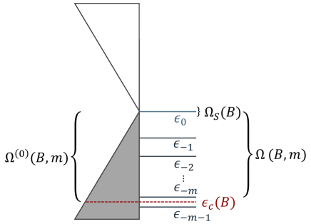
Further, we take an integration of Eq. (6) with an energy cut-off $\epsilon_{c}$ for $\Omega^{(0)}$, where $c\equiv-(m+x)$ as illustrated by Fig. 1. When we choose $x=1/2$, the finite integral of $\Omega^{(0)}$ from $\epsilon_{c}$ to 0 becomes $B$ dependent because of the $B$ dependece of $\epsilon_{c}$ as follows,

$$\Omega^{(0)}(B,m)\equiv\int_{\epsilon_{c}}^{0}\epsilon D(\epsilon)d\epsilon=-\frac{2}{3}C_{B}\left(m+\frac{1}{2}\right)^{3/2}.\\$$

(9)

The factor $(m+1/2)^{3/2}$ can be expanded by

$$\Big{(}m+\frac{1}{2}\Big{)}^{3/2}=m^{3/2}+\frac{3}{4}m^{1/2}+\frac{3}{32}m^{-1/2}+\mathcal{O}(m^{-3/2})$$

(10)

Using Eqs.  (7) to (10), we obtain $\Delta\Omega(B,m)\equiv\Omega(B,m)-\Omega^{(0)}(B,m)$ as follows:

	$\displaystyle\Delta\Omega(B,m)=$	$\displaystyle\Omega_{S}(B)-C_{B}\Bigg{[}\zeta\Big{(}-\frac{1}{2}\Big{)}-\frac{1}{48}m^{-1/2}$
		$\displaystyle+\mathcal{O}(m^{-3/2})\Bigg{]}.$		(11)

Since the two terms that are proportional to $m^{3/2}$ and $m^{1/2}$ are cancelled to each other, the second term of $\Delta\Omega(B,m)$ are converged to a finite value of $-C_{B}\zeta(-1/2)$ in the limit of $m\to\infty$. From Eq. (11), we obtain that $M$ of graphene for $\mathcal{E}\gg k_{B}T$ is given by $M(B)=\mathcal{C}_{1}T+\mathcal{C}_{2}\sqrt{B}$, where $\mathcal{C}_{1}$ and $\mathcal{C}_{2}$ are constants Pratama et al. (2021); Li et al. (2015).

It is important to note that we do not use zeta function regularization in Eq. (11). The value of zeta function $\zeta(-1/2)$ appears in the finite summation in Eq. (7). The role of $\Omega^{(0)}(B,m)$ is to cancel the terms proportional to $m^{3/2}$ and $m^{1/2}$ as a reference of energy. Thus we can justify the zeta function regularization for $\Omega(B)$ in which we do not need to consider $\Omega^{(0)}$ in Eq. (2). It should be mentioned that the selection of $x=1/2$ in Eq. (9) is essential to cancel the $m^{3/2}$ and $m^{1/2}$ terms. Generally, $x$ depends on $m$, which we discuss next.

Now, let us consider the case of weak-$B$ and high-$T$ limit for $M$ ($\mathcal{E}\ll k_{B}T$). In this limit, we need to consider the LLs from both valence and conduction bands. The $\Omega(B,m)$ and $\Omega(0,m)$ for $\mathcal{E}\ll k_{B}T$ are given by [See derivation in Section S1 B of the supplemental material]

$$\begin{split}\Omega(B,m)&=2\Omega_{S}^{(\mu)}+\sum_{\ell=0}^{\infty}C_{\ell}\left[\zeta(-\ell)-\zeta(-\ell,m+1)\right]\end{split}$$

(12)

and

$$\begin{split}\Omega^{(0)}(B,m)&=\sum_{\ell=0}^{\infty}C_{\ell}\frac{(m+x)^{\ell+1}}{\ell+1}\end{split}$$

(13)

where $\Omega_{S}^{(\mu)}=\ln{[1+\exp{(\beta\mu)}]}/(\pi{\ell_{B}}^{2}\beta)$ and $C_{\ell}$ is defined by

$\displaystyle C_{\ell}=\frac{4}{\pi{\ell_{B}}^{2}\beta}\frac{(\beta\mathcal{E})^{2\ell}}{(2\ell)!}\mathrm{Li}_{1-2\ell}(-e^{\beta\mu}),$

(14)

where $\mathrm{Li}_{s}(x)$ is polylogarithmic function. Therefore, the $\Delta\Omega(B,m)$ is given by a sum on $\ell$,

	$\displaystyle\Delta\Omega(B,m)=$	$\displaystyle~{}2\Omega_{S}^{(\mu)}+\sum_{\ell=0}^{\infty}C_{\ell}\Big{[}\zeta(-\ell)$
		$\displaystyle-\zeta(-\ell,m+1)-\frac{(m+x)^{\ell+1}}{\ell+1}\Big{]}.$		(15)

Similar to Eq. (8), we expand $\zeta(-\ell,m+1)$ in terms of $m$ as follows Olver et al. (2010):

	$\displaystyle\zeta(-\ell,m+1)\sim$	$\displaystyle-\frac{m^{\ell+1}}{\ell+1}-\frac{1}{2}m^{\ell}$
		$\displaystyle+\sum_{k=1}^{\infty}\begin{pmatrix}-\ell+2k-2\\ 2k-1\end{pmatrix}\frac{\mathcal{B}_{2k}}{2k}m^{\ell+1-2k},$		(16)

where $\mathcal{B}_{2k}$ is the Bernoulli number. In order to cancel the terms $m^{\alpha}$ for $\alpha\geqslant 0$ while keeping $\zeta(-\ell)$, we obtain $x$ as a function of $m$ in the finite region of $0<x(m)<1$ that satisfies the following equation for each $\ell$, ($\ell=0,1,2,\ldots)$,

	$\displaystyle\sum_{j=0}^{\ell}\begin{pmatrix}\ell+1\\ j\end{pmatrix}\frac{m^{j}}{\ell+1}x^{\ell+1-j}-\frac{1}{2}m^{\ell}$
	$\displaystyle+\sum_{k=1}^{\lfloor\frac{\ell+1}{2}\rfloor}\begin{pmatrix}-\ell+2k-2\\ 2k-1\end{pmatrix}\frac{\mathcal{B}_{2k}}{2k}m^{\ell+1-2k}$	$\displaystyle=0.$		(17)

If there exists a common solution of $x(m)$ for all $\ell$’s in Eq. (17), the zeta function regularization would be justified, which is not a trivial problem. As shown in Supplemental materials, the solutions of $x(m)$ for each $\ell$ are not the same. However, we always find any $x(m)$ in the region of $0<x(m)<1$ for all $\ell$’s and if we take a limit of $m\rightarrow\infty$, the solutions of $x(m)$ for all $\ell$’s are converging as follows

$\displaystyle x(m)\rightarrow\frac{1}{2}~{}~{}~{}\mathrm{for~{}all}~{}\ell,~{}~{}m\rightarrow\infty,$

(18)

[See Eqs. (S7) - (S16) of the supplemental material]. The meaning of Eq. (18) is that we can have the common $x$ in the limit of $m\to\infty$. By using Eq. (15), magnetization of graphene for $\mathcal{E}\ll k_{B}T$ is given by a linear response $M(B)\propto-(B/T)\mathrm{sech}^{2}(\beta\mu/2)$ whose result Pratama et al. (2021) is consistent with the formula of orbital susceptibilityMcClure (1956).

Now let us discuss the justification for the case of the Casimir force. The Casimir force is given by the derivative of the summation of zero-point energy of electro-magnetic wave between two metallic plates separated by a distance $d$,

$$F_{\textrm{C}}=-\frac{\partial\Delta V(d)}{\partial d},$$

(19)

Similar to Eq. (2), the summation of zero-point energy is given by $\Delta V(d)\equiv V(d)-V^{(0)}$, where $V(d)$ is the summation of zero-point energy when $d$ is sufficiently small compared with the one edge of the plates, $L$. $V^{(0)}$ is the reference energy of the vacuum. Similar to $\Omega^{(0)}$, the role of $V^{(0)}$ is to avoid the divergence for obtaining $F_{\textrm{C}}$. The $\Delta V(d)$ is expressed by [See Section S2 of the supplemental material for more detail derivation],

	$\displaystyle\Delta V(d)$	$\displaystyle=V(d)-V^{(0)}$
		$\displaystyle=-\frac{C}{d^{3}}\left(\sum\limits_{n=0}^{m}n^{3}-\int\limits_{0}^{m+x}dn~{}n^{3}\right),$		(20)

where constant $C$ is given by,

$\displaystyle C=\frac{L^{2}\pi^{2}\hbar c}{6}.$

(21)

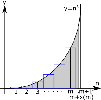
In Fig. 2, we illustrate for the summation in $V(d)$ and the integration in $V^{(0)}$, which is given by the shaded region. Similar to the cases of magnetization, we use the cut-off index $m$ in the summation and integration of Eq. (20). The $x$ in the cut-off for integration in Eq. (20) is determined so that the $\Delta V$ does not diverge for large $m$. Similar with the case of magnetization, we can consider the finite summation of Eq. (20) as the subtraction of the two zeta functions as follows:

	$\displaystyle\sum\limits_{n=0}^{m}n^{3}$	$\displaystyle=\zeta(-3)-\zeta(-3,m+1)$
		$\displaystyle=\zeta(-3)+\frac{m^{4}}{4}+\frac{m^{3}}{2}+\frac{m^{2}}{2},$		(22)

where Eq. (22) is obtained when we use the fact that $m\rightarrow\infty$ in evaluating the $\zeta(-3,m+1)$. However, the divergent terms in $V(d)$ and $V^{(0)}$ are cancelled to each other when we select $x=-m+m\sqrt{1+1/m}\approx 1/2+\mathcal{O}(m^{-1})$. In order to show how $\Delta V(d)$ is converged in the limit of $m\to\infty$, the $x$ is expanded for $1/m\ll 1$ up to fourth order [See Eq. (S23) of the supplemental material]. Finally we get $\Delta V(d)$ as follows:

$\displaystyle\Delta V(d)=-\frac{C}{d^{3}}\left[\zeta(-3)+\frac{7}{256m}+\mathcal{O}\left({m^{-2}}\right)\right],$

(23)

where the terms in the bracket converge to $\zeta(-3)$ for increasing $m$. Therefore, the $F_{\textrm{C}}$ is obtained from Eq. (19) as follows:

$\displaystyle F_{\textrm{C}}=-\frac{3C}{d^{4}}\zeta(-3),$

(24)

where $\zeta(-3)=1/120$. Thus, the two values of zeta functions in Eq. (22) has a physical meaning of the force. Once again, we do not use the zeta function regularization for obtaining the Casimir force, instead we consider a finite summation on $n^{3}$ in Eq. (22).

It is noted that the energies are measured from reference energies in the both cases of magnetization $\Delta\Omega$ and Casimir effect $\Delta V$. The reference energies are expressed by integration. In the Section S3 of the supplemental material, we also justify the zeta-function regularization when we use the definition of differential coefficient at a finite $B$

$$M(B)=-\left.\frac{\partial\Omega(B)}{\partial B}\right|_{B}=-\lim_{\delta B\to 0}\frac{\Omega(B+\delta B)-\Omega(B)}{\delta B}.$$

(25)

We can show that the $\Delta\Omega(B)$ (or $\Delta V(d)$) also converge to the corresponding zeta function by similar treatment.

In conclusion, zeta function regularization is justified by using the finite summation of energy up to finite discrete number $m$ that is subtracted by the reference energy. The zeta function appears as the remaining term when we subtract two diverging energies. The present treatment can be generally applied for any divergent summation in physics, which should be useful for understanding the zeta function regularization.

FRP acknowledges MEXT scholarship. MSU and RS acknowledge JSPS KAKENHI Grant Number JP18H01810.

References

- Riemann (1859) B. Riemann, Ges. Math. Werke und Wissenschaftlicher Nachlaß 2, 145 (1859).
- Elizalde (2012) E. Elizalde, Ten physical applications of spectral zeta functions, Vol. 855 (Springer, 2012).
- Elizalde (2021) E. Elizalde, Universe 7, 5 (2021).
- Tao (2013) T. Tao, Compactness and contradiction (American Mathematical Society Providence, RI, 2013).
- Casimir (1948) H. B. Casimir, in Proc. Kon. Ned. Akad. Wet., Vol. 51 (1948) p. 793.
- Lamoreaux (1997) S. K. Lamoreaux, Physical Review Letters 78, 5 (1997).
- Klimchitskaya et al. (2009) G. Klimchitskaya, U. Mohideen, and V. Mostepanenko, Reviews of Modern Physics 81, 1827 (2009).
- Rodriguez et al. (2011) A. W. Rodriguez, F. Capasso, and S. G. Johnson, Nature photonics 5, 211 (2011).
- Sushkov et al. (2011) A. Sushkov, W. Kim, D. Dalvit, and S. Lamoreaux, Nature Physics 7, 230 (2011).
- Bressi et al. (2002) G. Bressi, G. Carugno, R. Onofrio, and G. Ruoso, Physical review letters 88, 041804 (2002).
- Decca et al. (2007) R. Decca, D. López, E. Fischbach, G. Klimchitskaya, D. Krause, and V. Mostepanenko, Physical Review D 75, 077101 (2007).
- Hawking (1977) S. W. Hawking, in Euclidean quantum gravity (World Scientific, 1977) pp. 114–129.
- Escobar et al. (2020) C. Escobar, E. Chan-López, and A. Martín-Ruiz, Physical Review D 101, 046023 (2020).
- Dalvit et al. (2011) D. Dalvit, P. Milonni, D. Roberts, and F. Da Rosa, Casimir physics, Vol. 834 (Springer, 2011).
- Svaiter and Svaiter (1993) B. Svaiter and N. Svaiter, Physical Review D 47, 4581 (1993).
- Ghosal et al. (2007) A. Ghosal, P. Goswami, and S. Chakravarty, Physical Review B 75, 115123 (2007).
- Pratama et al. (2021) F. Pratama, M. S. Ukhtary, and R. Saito, Physical Review B 103, 245408 (2021).
- Li et al. (2015) Z. Li, L. Chen, S. Meng, L. Guo, J. Huang, Y. Liu, W. Wang, and X. Chen, Physical Review B 91, 094429 (2015).
- Olver et al. (2010) F. W. Olver, D. W. Lozier, R. F. Boisvert, and C. W. Clark, NIST handbook of mathematical functions hardback and CD-ROM (Cambridge university press, 2010).
- McClure (1956) J. McClure, Physical Review 104, 666 (1956).