JWST observations of K2-18b can be explained by a gas-rich mini-Neptune with no habitable surface
Abstract
JWST recently measured the transmission spectrum of K2-18b, a habitable-zone sub-Neptune exoplanet, detecting CH4 and CO2 in its atmosphere. The discovery paper argued the data are best explained by a habitable “Hycean” world, consisting of a relatively thin H2-dominated atmosphere overlying a liquid water ocean. Here, we use photochemical and climate models to simulate K2-18b as both a Hycean planet and a gas-rich mini-Neptune with no defined surface. We find that a lifeless Hycean world is hard to reconcile with the JWST observations because photochemistry only supports part-per-million CH4 in such an atmosphere while the data suggest about of the gas is present. Sustaining %-level CH4 on a Hycean K2-18b may require the presence of a methane-producing biosphere, similar to microbial life on Earth billion years ago. On the other hand, we predict that a gas-rich mini-Neptune with solar metallicity should have 4% CH4 and nearly 0.1% CO2, which are compatible with the JWST data. The CH4 and CO2 are produced thermochemically in the deep atmosphere and mixed upward to the low pressures sensitive to transmission spectroscopy. The model predicts H2O, NH3 and CO abundances broadly consistent with the non-detections. Given the additional obstacles to maintaining a stable temperate climate on Hycean worlds due to H2 escape and potential supercriticality at depth, we favor the mini-Neptune interpretation because of its relative simplicity and because it does not need a biosphere or other unknown source of methane to explain the data.
1 Introduction
Whether or not life is abundant in the galaxy depends on the frequency of habitable worlds. The Kepler era of exoplanet exploration revealed that close-in sub-Neptunes ( ) have high occurrence rates (Fulton & Petigura, 2018). These planets have bulk densities that can be explained by several planetary models that range from a massive H2 atmosphere similar to Neptune’s, to a thin hydrogen atmosphere (e.g., bar) overlying a H2O-rich interior. Researchers have suggested that H2O-rich sub-Neptunes could have habitable surface oceans provided that the climate is suitable for liquid water (Madhusudhan et al., 2021). These so-called “Hycean” worlds, if they exist, have the potential to be among the most common habitable planetary environments.
Perhaps the best known Hycean world candidate is the sub-Neptune K2-18b (8.63 M⊕, 2.61 R⊕; Benneke et al., 2019)), which was recently observed by the James Webb Space Telescope (i.e., JWST; Madhusudhan et al., 2023b). The transmission spectrum reveals strong evidence for CH4 and CO2 in a H2-rich atmosphere. Furthermore, JWST did not detect NH3, H2O or CO. Madhusudhan et al. (2023b) argued the data are best explained by a habitable Hycean world because, according to past photochemical studies, such a planet can be consistent with the NH3 non-detection (Tsai et al., 2021a; Yu et al., 2021; Madhusudhan et al., 2023a; Hu et al., 2021). Ammonia is instead expected on a mini-Neptune with a massive hydrogen atmosphere (e.g., Yu et al., 2021; Hu et al., 2021). Furthermore, Madhusudhan et al. (2023b) favored a Hycean world because their retrieved abundances for CH4 and CO2 are broadly compatible with photochemical modeling predictions made by Hu et al. (2021) for a Hycean K2-18b.
Here, we use 1-D photochemical and climate models to revisit the past calculations (Hu et al., 2021; Yu et al., 2021; Tsai et al., 2021a) that support a habitable ocean-world interpretation of the data. We simulate K2-18b as a Hycean planet to determine whether the CH4 and CO2 suggested by JWST are photochemically stable in such an atmosphere. Our Hycean models consider both a lifeless and inhabited planet, the latter represented by a primitive microbial biosphere that influence atmosphere chemistry. We also model K2-18b as a gas-rich mini-Neptune with a deep atmosphere. By comparing our simulations to the JWST data, and considering the relative complexities for each simulated composition, we suggest the most likely planetary model for K2-18b.
2 Methods
2.1 Hycean worlds
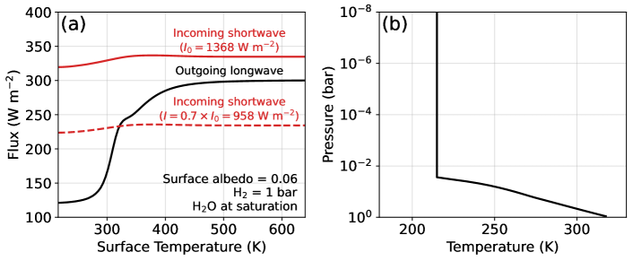
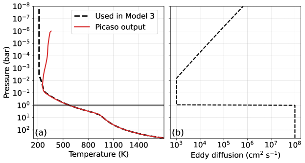
To simulate a Hycean K2-18b, we first modeled a pressure-temperature (P-T) profile using the climate code contained within the Photochem software package (Wogan et al., 2023). The climate model uses correlated-k radiative transfer with opacities detailed in Appendix D of Wogan et al. (2023). The code constructs P-T profiles assuming the lower atmosphere follows a moist-pseudo adiabat connected to an isothermal stratosphere. For K2-18b, we assume a 215 K stratosphere following Hu (2021). Our approach can consider any number of condensing species (e.g., Graham et al., 2021), but H2O is the most important condensable for a habitable K2-18b.
For a Hycean K2-18b, we nominally assume a 1-bar H2-dominated atmosphere with a water-saturated troposphere to facilitate comparison with previous work (Hu et al., 2021; Madhusudhan et al., 2023a; Innes et al., 2023). For such a composition, our cloud-free climate model predicts that K2-18b would not be habitable because the surface temperature would exceed the critical point of H2O (Figure 1a), consistent with past studies (Innes et al., 2023; Scheucher et al., 2020). However, it has been suggested that high-altitude clouds or hazes could potentially reflect short wave radiation allowing for a cooler climate (Madhusudhan et al., 2021; Piette & Madhusudhan, 2020). To approximate the cooling effects of clouds in our cloud-free climate simulations, following Hu et al. (2021), we arbitrarily reduce the incoming solar radiation by 30% which permits a K surface (Figure 1a). We adopt this habitable P-T profile, shown in Figure 1b, for all Hycean scenarios. Our photochemical simulations include up to %-level CH4 and CO2, but the Figure 1b P-T profile ignores their greenhouse contribution. For this analysis, this is justified because the climate of a Hycean K2-18b is uncertain, and our climate model predicts the surface temperature would increase by K when accounting for CH4 and CO2.
With our estimated P-T profile (Figure 1b), we then simulate steady-state photochemistry using Photochem (Wogan, 2024a). The photochemical model contained in Photochem solves a system of partial differential equations approximating molecular transport in the vertical direction and the effect of chemical reactions, photolysis and condensation. We have made several updates to the reaction network and thermodynamic data originally published in Wogan et al. (2023). We improved the kinetics and thermodynamics of , and related species, all of which are detailed in Appendix Table A1. For key reactions, we nominally adopt new kinetics following Xu et al. (2015), but we also consider alternative rates from Klippenstein (2023). Theses updates are important for estimating photochemical methane production on Hycean worlds as discussed in Section 3.1. We have also updated our H2O and H2 photolysis data (Appendix Table A1). The updated network is available on Zenodo (see the “.yaml” files in the “input/” folder of Wogan (2024b)). Because the UV spectrum of K2-18 has not been measured, we instead use the UV spectrum of GJ 176 measured by the MUSCLES survey for our photochemical calculations (France et al., 2016) following the Hu et al. (2021) analysis.
| Model type | Model # | Metallicity | Lower boundary condition | ||||
| N2 | CO2 | CH4 | CO | ||||
| Lifeless Hycean | 1 | - | |||||
| Inhabited Hycean | 2 | - | |||||
| Mini-Neptune | 3 | Figure A1b | solar | chemical equilibrium | |||
| The vertically-constant eddy diffusion coefficient in cm2 s-1 All Hycean models include cm s-1 deposition velocities for HCN and HCCCN (Wogan et al., 2023), and impose a cm s-1 deposition velocity for C2H6 (Hu et al., 2021). The mini-Neptune case has a solar C/O ratio and a 60 K intrinsic temperature. The variable indicates a fixed lower-boundary mixing ratio, indicates a fixed surface flux in molecules cm-2 s-1, and indicates a surface deposition velocity in cm s-1. If a fixed surface flux is specified, then the deposition velocity is zero. In Hycean simulations, unspecified molecules have a zero-flux lower boundary condition. In the mini-Neptune case, we assume fixed lower boundary conditions at chemical equilibrium for molecules with equilibrium concentrations mixing ratio. For lower concentration molecules, we permit molecules to mix into the deep atmosphere ( bar) with a deposition velocity , where is scale height, following past works (Moses et al., 2000). | |||||||
2.2 Mini-Neptune world
We additionally model K2-18b as a gas-giant mini-Neptune with no habitable surface. We take the same approach as Hu (2021) and simulate the massive hydrogen atmosphere over two stages: The first considers the deep atmosphere (500 to 1 bar), and the second simulates the upper atmosphere (1 to bar). The lower atmosphere stage captures the equilibrium-to-disequilibrium transition (i.e., gas quenching) that occurs deep in a gas-giant atmosphere (e.g., Zahnle et al., 2016), while the upper atmosphere model approximates the impact of UV photolysis and gas condensation on composition.
For the first stage, we use the PICASO climate model (Mukherjee et al., 2023) to generate a P-T profile with opacities appropriate for a solar metallicity with a solar C/O at chemical equilibrium assuming a geothermal heat flow consistent with an intrinsic temperature () of 60 K (Hu, 2021). Note that the intrinsic temperature affects the upper atmosphere abundance of gases such as CH4 (Fortney et al., 2020). We discuss this dependence in Section 3.2, but leave a full parameter space exploration for future work. Next, using the P-T profile, we do a full kinetics simulation with the Photochem model between 500 bar and 1 bar using our network of reversible reactions described previously (Section 2.1). We fix the lower boundary to chemical equilibrium composition, and allow the kinetics model to predict the chemical equilibrium-to-disequilibrium transition. The deep atmosphere adopts an altitude-independent eddy diffusion coefficient of cm2 s-1 following Hu (2021).
In the second stage we simulate K2-18b’s upper atmosphere using results from the first stage as lower boundary conditions. We do not use the PICASO P-T profile above 1 bar because PICASO assumes the entire atmospheric profile is at chemical equilibrium which would not be the case for the cool upper atmosphere of K2-18b. The chemical equilibrium assumption creates a stratospheric inversion in the P-T profile from greenhouse gases such as CH4. Furthermore, PICASO assumes a dry convective lapse rate but the P-T profile in much of the upper troposphere should follow a moist-pseudo adiabat because of water condensation. As an alternative to PICASO, we extrapolate the P-T profile above the 1 bar level by drawing an adiabat upwards using the Photochem climate model until it intersects an isothermal 215 K stratosphere. Appendix Figure A1a compares the PICASO profile to the modified profile that we adopt. Finally, using the modified P-T profile, we compute the photochemical steady-state of the upper atmosphere (1 to bar) to predict its composition. At the lower boundary, we fix all gas concentrations to the values predicted at the 1 bar level of the lower atmosphere kinetics simulation described in the previous paragraph. The upper atmosphere simulation assumes a Jupiter-like eddy diffusion profile as used in Hu (2021) (Appendix Figure A1b).
2.3 Transmission spectra
We use the PICASO code (Batalha et al., 2019) to compute the transmission spectra of simulated Hycean and mini-Neptune atmospheres adopting the R=60,000 resampled opacities archived on Zenodo (Batalha et al., 2022). The main text presents clear-sky spectra because the JWST data do not favor high altitude clouds. The Appendix shows the spectral effects of water, elemental sulfur (S2 and S8) and hydrocarbon clouds and hazes.
3 Results
3.1 Hycean worlds
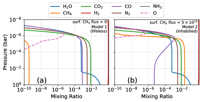
To investigate K2-18b as a Hycean world we first consider an uninhabited planet. Our nominal simulation, called “model 1”, assumes a 1 bar H2-dominated atmosphere, 0.8% CO2 fixed at the surface, and other settings and boundary conditions detailed in Table 1. We choose 0.8% CO2 because it is the median concentration implied by the JWST spectrum (Madhusudhan et al., 2023b). Methane has a zero-flux lower boundary condition, therefore all accumulated CH4 is the result of the photochemical reduction of CO2 to CH4. Figure 2a shows the steady-state composition of the model 1 atmosphere as a function of pressure revealing that only 0.4 part-per-billion (ppb) CH4 is photochemically stable. Methane is slowly produced by the following sequence of reactions:
| (1a) | ||||
| (1b) | ||||
| (1c) | ||||
| (1d) | ||||
| (1e) | ||||
| (1f) | ||||
| (1g) | ||||
| (1h) | ||||
| (1, net) | ||||
By analyzing column-integrated reaction rates we have determined that Reaction (1d) is the rate-limiting step. Another important path with the same net reaction replaces both reactions involving CH3O with alternatives that depend on the isomer H2COH:
| (2) | ||||
| (3) |
Methane is effectively destroyed by photolysis followed by several oxidizing reactions:
| (4a) | ||||
| (4b) | ||||
| (4c) | ||||
| (4d) | ||||
| (4e) | ||||
| (4f) | ||||
| (4, net) | ||||
In H2-rich solar system atmospheres (e.g., Saturn’s), methane has a long lifetime to destruction because, after photolysis (Reaction (4a)), it recombines: (Moses et al., 2000). The same recombination is inefficient in model 1 because, unlike the gas-giants in the solar system, model 1 has substantially more oxidizing gases like H2O. In particular, water vapor photolysis at Ly- wavelengths ( nm) produces oxygen atoms (Reaction (4b), Slanger & Black, 1982) that rapidly oxidize CH3 before CH4 is reformed. Methyl is also destroyed by atomic oxygen sourced from a sequence of reactions involving CO2 photolysis: , , and which has the net reaction . Overall, efficient methyl oxidation in additional to slow CH4 production (Reaction path (1)), results in only trace amounts of atmospheric CH4.
Our result that CH4 cannot accumulate in model 1 is not sensitive to many model assumptions. For example, we have recomputed model 1 with vertically constant between and cm2 s-1, N2 concentrations () between ppm and 1%, and troposphere relative humidities () spanning 0.1 to 1. Within this parameter space, our photochemical code predicts the maximum stable CH4 concentration is only 4 ppb for cm2 s-1, ppm, and . As an additional test, we recomputed model 1 using alternative rates for Reactions 1d and 2 derived by Klippenstein (2023) using ab initio methods. Klippenstein (2023) predicts that these important rate-limiting reactions are faster than the Xu et al. (2015) rates we nominally assume (Appendix Table A1) at the temperatures and pressures relevant to Hycean atmospheres. Despite this difference, our model using the Klippenstein (2023) rates predicts only 32 ppb CH4.
Up to this point, we have modeled K2-18b as a habitable, yet uninhabited planet. Now we consider an inhabited case, which we refer to as model 2. Model 1 imposes the surface concentration of H2, CO2 and N2, but most all other gases, including CH4 and CO, are dictated by photochemistry. If K2-18b is a Hycean world inhabited by microbial life then CH4 and CO could be biologically modulated gases like they were on the anoxic Archean Earth (Kharecha et al., 2005; Wogan & Catling, 2020; Thompson et al., 2022). Chemosynthetic methanogens can consume H2 and CO2 for energy, producing methane as a waste gas:
| (5) |
CO is also food for acetogenic microbes:
| (6) |
The produced could have been food for acetotrophic methanotrophs (). Model 2 simulates K2-18b as a Hycean world with boundary conditions representing biological influence from these early Archean metabolisms (Table 1). To model methanogenic life, we impose a surface CH4 flux needed to replicate the %-level concentration implied by the JWST data, which ended up being half the modern Earth’s biological methane flux ( molecules cm-2 s-1, Jackson et al., 2020). We also add a CO deposition velocity of cm s-1 to approximate the influence of CO-consuming acetogens (Reaction (6), Kharecha et al., 2005). At photochemical steady-state, model 2 has 2% CH4 and a CO mixing ratio at the surface (Figure 2b).
With a methanogenic biosphere, CH4 can accumulate to the %-levels suggested by recent JWST observations (Madhusudhan et al., 2023b). In contrast, on an uninhabited Hycean K2-18b, CH4 should be at only ppb-levels (model 1) because large concentrations can not accumulate photochemically and other non-biological sources of methane seem implausible (Section 4).
3.2 Mini-Neptune world
Figure 3 shows K2-18b modeled as a gas-giant mini-Neptune with no habitable surface (i.e., model 3 in Table 1). Deep in the atmosphere, at 500 bar and 1700 K, fast reactions enforce chemical equilibrium for our assumed composition of solar metallicity with a solar C/O ratio. As gases mix upward to lower pressures and temperatures, reactions slow, causing an equilibrium-to-disequilibrium transition (i.e., gas quenching). N2 and NH3 chemistry quenches near 200 bar and K, and the CO2-CO-CH4 system fails to maintain equilibrium near 100 bar and K. These quench points are broadly consistent with Hu (2021) who constructed similar mini-Neptune models of K2-18b.
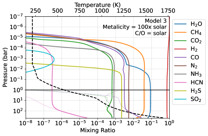
Quenched gases from the deep atmosphere mix upward to Model 3’s stratosphere where they are relevant to transmission spectroscopy. The atmosphere has 4% CH4 along with 0.06% CO2 at 1 mbar, which is broadly consistent with recent JWST observations (Madhusudhan et al., 2023b). Water vapor condensation between 0.07 bar and 4 mbar reduces its concentration, causing only 0.3% of the gas to be present at 1 mbar. At the same pressure level, there is also 0.3% CO and 0.07% NH3. Only trace photochemically produced SO2 is present ( mixing ratio) as most all sulfur is photochemically processed to S2 and S8 in the lower atmosphere where it condenses out (Zahnle et al., 2016).
We additionally tested the sensitivity of Model 3 to the assumed intrinsic temperature ( K), as this parameter can impact deep atmosphere quenching and the resulting stratospheric abundances of CH4, CO2, and CO (Fortney et al., 2020; Tsai et al., 2021b). Larger (e.g, 100 K) drives an increase in CO that is hard to reconcile with JWST observations. For lower values (e.g., 30 K), our model does not produce enough CO2 to explain the JWST data. Future abundance constraints from JWST offer an exciting avenue to study K2-18b’s internal temperature and thermal evolution. We leave detailed exploration of this topic to a future study.
3.3 Transmission spectra and comparison to JWST data
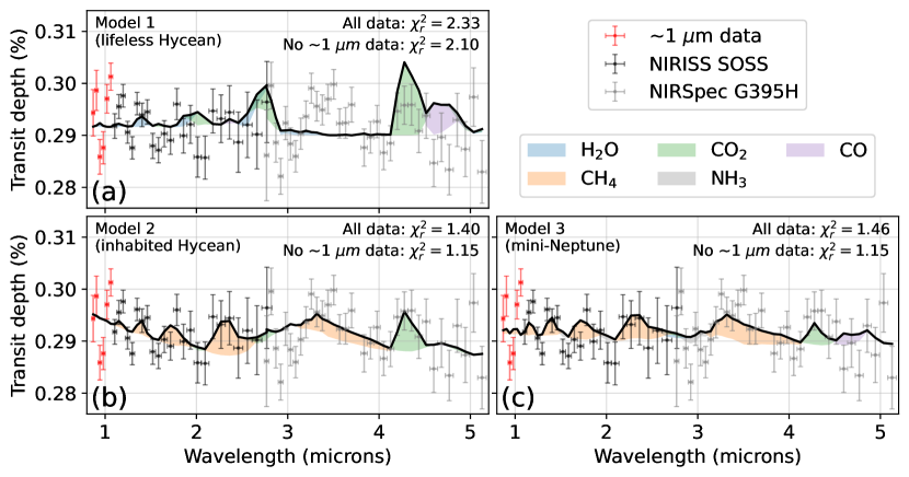
Figure 4 shows the simulated clear-sky transmission spectra of three scenarios for K2-18b compared to JWST NIRISS and NIRSpec observations: A lifeless Hycean planet (model 1), a Hycean world inhabited by an Archean-like biosphere (model 2) and a solar metallicity mini-Neptune with no habitable surface (Model 3). In all cases, we allow the simulated spectra to have an offset between the NIRISS and NIRSpec data as to best fit the observations, motivated by Madhusudhan et al. (2023b).
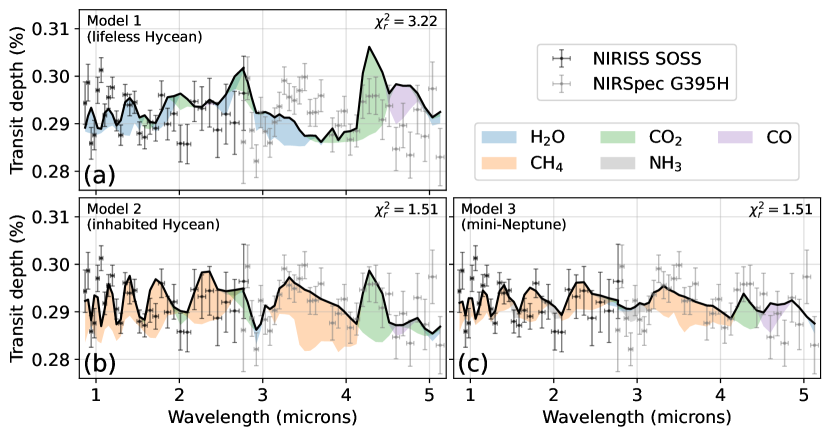
JWST data rules out model 1 () because the lifeless Hycean world does not have enough methane ( ppb, Figure 2) to explain the observed CH4 absorption shortwards of m. On the other hand, the data do not strongly exclude an inhabited Hycean world (model 2, ). Model 2 fits the CH4 and CO2 spectral features in the data because it has 2% of biologically-produced methane along with 0.8% CO2.
However, an inhabited Hycean world is not required to explain the data. Our model of a gas-giant mini-Neptune (model 3) has a comparable fit () largely because of its 4% CH4 and 0.06% CO2 at mbar. The spectra show small H2O absorption because water vapor is cold trapped at mbar (Figure 3). Also, NH3 has small absorption features at 1.5, 2, and 3 m. Madhusudhan et al. (2023b) used the JWST data to argue for an NH3 upper bound of at 95% confidence assuming a vertically constant NH3 concentration. At 1 mbar, our mini-Neptune model has NH3, but photolysis rapidly diminishes the gas’s concentration towards lower pressures (see Figure 3). Using a transmission contribution function (Equation 8 in Mollière et al. (2019)) we find that the 3 m NH3 feature (Figure 4c) is sensitive to pressures between and bar where the ammonia concentration is between and mixing ratio. While a direct comparison is challenging, our modeled heterogeneous NH3 profile appears broadly compatible with the vertically constant upper bound derived by Madhusudhan et al. (2023b).
Models 2 and 3, and the retrievals presented in Madhusudhan et al. (2023b), are not able to reproduce the apparent large absorption feature near m (red points in Appendix Figure A2). Disregarding these six data points reduces values for both model 2 and 3 to about . Future visits with NIRISS SOSS will be valuable to determine whether the scatter near m is physical or instrumental.
Our conclusion that the data strongly rule out model 1 but not model 2 or 3 is unchanged when including various aerosol opacities (Appendix Figure A2). Accounting for aerosols, the model 1 simulated spectrum remains a poor fit () when compared to model 2 and 3 ().
4 Discussion
4.1 Reconciling our lifeless Hycean model with past research
Hu et al. (2021) pioneered the use of photochemical models to simulate K2-18b as a lifeless Hycean planet. They consider a 1 bar H2 atmosphere, 1% N2, a comparable P-T profile to ours (Figure 1b), and CO2 concentrations between 400 ppm and 10%. In all scenarios, they predict the photochemical accumulation of %-levels CH4, which contrasts with the ppb-level CH4 we compute in very similar scenarios (e.g., model 1). There are two reasons our results differ. First, Hu et al. (2021) assumed that the photolysis of H2O produces only OH + H. However, we demonstrate here that the seemingly minor channel that produces O + H + H (Reaction 4b) is important for CH4 destruction in K2-18b’s atmosphere. To verify this insight, we have rerun the 400 ppm-CO2 model of Hu et al. (2021) using their photochemical network and code, and with the sole inclusion of the O + H + H channel the steady-state CH4 drops from 1% to mixing ratio.
The second reason our results differ has to do with CH4 production. Hu et al. (2021) modeled Reaction (1d), a critical step to methane formation, with its high-pressure limit rate constant. This approach can accurately estimate the rate at high pressures ( bar) but substantially over predicts the rate at bar where third body collisions are more scarce. We have also rerun the 400 ppm-CO2 model of Hu et al. (2021) using their code, now also with the Xu et al. (2015) pressure-dependent rate constant in Appendix Table A1, and find that the steady-state CH4 mixing ratio further drops to . This concentration is broadly consistent with model 1 shown in Section 3.1, given remaining subtle differences in the temperature, diffusivity, and radiative transfer.
To further test the above explanation, we have also used the Photochem code to reproduce the 400 ppm-CO2 case in Hu et al. (2021). Adopting their boundary conditions, P-T profile, and eddy diffusion profile, our chemical network predicts mixing ratio CH4 at steady state. When we perform the same simulation but use the Hu et al. (2021) pressure-independent rate for Reaction (1d), our code predicts mixing ratio CH4 should accumulate. When Photochem also omits the O + H + H branch of H2O photolysis, the CH4 concentration further rises to . These Photochem results are generally compatible with our Hu et al. (2021) code calculations for the same experiments.
Furthermore, Madhusudhan et al. (2023a) was unable to reproduce Hu et al. (2021) using an independent photochemical model and network. “Case 11” in Madhusudhan et al. (2023a) is very similar to the 10%-CO2 case in Hu et al. (2021), representing a 1 bar uninhabited Hycean world (i.e., zero-flux boundary conditions for CH4 and CO). At photochemical steady-state, Madhusudhan et al. (2023a) finds that only 55 ppb CH4 should persist, which aligns with our conclusion that methane should be a trace gas (e.g., ppm) on such a planet.
Yu et al. (2021) and Tsai et al. (2021a) also simulated a 1 bar H2-dominated atmosphere on K2-18b, but instead with a hot K rocky surface (i.e., no habitable ocean). They find that to 1% CH4 can accumulate alongside of CO2 and CO. We have done similar simulations with the Photochem code and found that larger CH4 concentrations are stable in this case because the hot K surface breaks down the kinetic barriers to CH4 production. For example, when temperature is increased from 320 K to 600 K, the rate of the reaction increases by about six orders of magnitude while Reaction (2) increases by a factor of . In contrast, methane production is far more kinetically inhibited on a Hycean planet with a habitable 320 K surface (e.g., model 1). Furthermore, the 1 bar scenarios in Yu et al. (2021) and Tsai et al. (2021a) with rocky surfaces can be ruled out because such a planet would be denser than K2-18b’s observed density. To explain the planet’s mass and radius with only a silicate interior and a H2-rich envelope, interior modeling suggests the atmosphere needs to be bars thick (Madhusudhan et al., 2020, 2023b).
4.2 Can CH4 accumulate from non-photochemical abiotic processes?
Substantial methane from non-photochemical abiotic processes is hard to sustain on a Hycean planet. To explain K2-18b’s density, a Hycean world needs a large high-pressure ice layer that separates deep rocky material from the surface water ocean (Madhusudhan et al., 2021). Water-rock reactions and subsequent transport of CH4 is conceivable (Thompson et al., 2022), but improbable in this case since the high overburden pressure of water and ice inhibits the production of fresh crust to be hydrated (Krissansen-Totton et al., 2021). Moreover, the shutdown of melting of deep-subsurface silicates also precludes the possibility of volcanic CH4 (Krissansen-Totton et al., 2021; Noack et al., 2016; Kite & Ford, 2018). Massive asteroid impacts on the early Earth may have made transient atmospheric methane (Wogan et al., 2023). However, ephemeral impact-induced CH4 is unlikely on K2-18b because the planet is billion years old (Guinan & Engle, 2019), while substantial bombardment is expected to end within the first several hundred million years of planet formation (Lichtenberg & Clement, 2022).
4.3 Inhabited Hycean vs. mini-Neptune: evaluating model complexity
Our results suggest that both an inhabited Hycean world (model 2) or a mini-Neptune with a massive H2 atmosphere (model 3) are not strongly ruled out by the JWST data (). However, in addition to evaluating the fit to the data, we also must assess the relative complexity of each scenario. The inhabited Hycean world (model 2) requires a cool habitable surface, but models suggest that a cloud-free -bar H2-rich atmosphere should trigger a hot runway greenhouse (Figure 1, Innes et al., 2023; Pierrehumbert, 2023). A supercritical steam-dominated atmosphere would have a small scale height incompatible with JWST observations (Scheucher et al., 2020). For a temperate surface, climate codes need to assume the presence of high-altitude clouds or hazes that scatter away starlight (Madhusudhan et al., 2021; Piette & Madhusudhan, 2020).
Beyond this climate paradox, bar of H2 may also be susceptible to rapid escape driven by extreme-ultraviolet radiation (i.e., XUV, Hu et al., 2023). Even if a 1 bar H2 atmosphere could withstand modern XUV radiation, K2-18b likely experienced exceptionally high XUV fluxes during the host M star’s pre-main sequence, potentially driving hundreds of bars of H2 loss (Luger et al., 2015), as so a remnant thin bar atmosphere would be highly fortuitous. As noted previously, replenishing H2 with volcanism would be unlikely on a Hycean K2-18b because rocky material in the deep subsurface would be at pressures too high for melting and outgassing (Kite & Ford, 2018; Noack et al., 2016).
In contrast, our model of a gas-giant mini-Neptune (model 3) is relatively straightforward. For a solar composition, solar C/O, and K, which are physically plausible given K2-18b’s mass, a spectrum broadly consistent with the JWST data falls out of our model. Unlike a Hycean world, a mini-Neptune does not require a biosphere to explain the disequilibrium combination of atmospheric CH4 and CO2. Instead, these gases emerge in model 3 from deep-atmosphere quenching (Figure 3). Even though both an inhabited Hycean world and a mini-Neptune are allowed by JWST data, the climate of a Hycean world and the atmosphere’s resilience to escape is hard to explain, so we favor the mini-Neptune model for its simplicity.
While our mini-Neptune simulation is relatively simple, it makes assumptions that should be investigated with more sophisticated modeling. Namely, we simulate the planet’s climate (Figure 3) using a two-stage approach that is not fully self-consistent with photochemistry (Section 2.2), yet an accurate tropopause temperature is important for predicting whether H2O cold-trapping can reproduce the JWST non-detection of water vapor. The water vapor cold trap would be better approximated by a model that is self-consistent with photochemistry and accounts for the possibility of convection inhibition (Innes et al., 2023). The need for a H2O cold trap is not unique to a mini-Neptune planet. A Hycean world would also need substantial water condensation to explain the H2O non-detection. An additional shortcoming of this study is that we only consider one mini-Neptune scenario with a composition of solar metallicity, and solar C/O. Further modeling could tune metallicity and the C/O ratio to get an even better fit to the JWST observations.
4.4 Future observations of K2-18b
Clearly distinguishing between the inhabited Hycean and mini-Neptune interpretations with future JWST observations will be challenging. Ammonia should be unique to a mini-Neptune K2-18b (Figure 3, Yu et al., 2021; Tsai et al., 2021a; Madhusudhan et al., 2023a; Hu et al., 2021). However, even if future observations are unable to detect NH3, this would not necessarily prove the inhabited Hycean case. In our mini-Neptune model, the NH3 features act to fill CH4 spectral windows (Figure 4). This small ammonia absorption is difficult to distinguish from clouds which have a similar effect on the spectrum (Figure A2). Additionally, there are several reasons why ammonia could be less abundant on a mini-Neptune K2-18b than we have estimated, making a detection even more challenging. Hu (2021) predicted stratospheric NH3 could be photochemically depleted to undetectable concentrations ( ppm) on a gas-rich K2-18b if tropospheric mixing is slow ( cm2 s-1). Also, nitrogen could dissolve into a magma ocean at the base of a thick H2-rich envelope, preventing a large observable NH3 abundance in the upper atmosphere (Shorttle et al., 2024).
An inhabited Hycean world could be identified with the detection of a biogenic gas. Madhusudhan et al. (2023b) found weak evidence for dimethyl sulfide (DMS) in K2-18b’s transmission spectrum, a gas almost exclusively produced by life on Earth (Catling et al., 2018). If DMS is detected with statistical significance, it might be difficult to account for its presence without a biosphere on a Hycean planet.
5 Conclusions
Recent JWST observations of K2-18b (Madhusudhan et al., 2023b), a habitable-zone sub-Neptune exoplanet, revealed the presence of atmospheric CH4 and CO2. Madhusudhan et al. (2023b) suggested that the data are best explained by a habitable “Hycean” world. Our photochemical and climate simulations of K2-18b as a lifeless Hycean world suggest such a planet would have ppb-level CH4 because the gas is rapidly destroyed by photolysis and subsequent oxidizing reactions. Lacking substantial CH4, an uninhabited Hycean planet cannot explain these recent JWST observations, which suggest of the gas is present (Madhusudhan et al., 2023b). However, there are still two scenarios that fit the JWST observations equally well according to a metric: a Hycean world inhabited by methanogenic life, or a mini-Neptune with no defined surface. The latter case is less complex and requires fewer assumptions.
Specifically, an inhabited Hycean K2-18b has the following difficulties:
-
•
To explain the CH4 detected by JWST, a Hycean planet needs biogenic CH4 or some other unknown source of the gas to maintain it against photochemical destruction.
-
•
Models predict that a stable temperate climate is challenging on a Hycean K2-18b. Such a planet is expected to experience a steam runaway greenhouse (Figure 1; Innes et al., 2023; Scheucher et al., 2020; Pierrehumbert, 2023), unless starlight can be reflected away by clouds (Madhusudhan et al., 2021; Piette & Madhusudhan, 2020).
- •
On the other hand, the benefits of the mini-Neptune case are:
-
•
The CH4 and CO2 detected by JWST can be broadly explained by deep-atmosphere thermochemical quenching for a solar metallicity, solar C/O, and 60 K intrinsic temperature.
-
•
Deep atmosphere kinetics also predicts NH3 and CO abundances generally compatible with the JWST non-detections of each gas.
-
•
The lack of H2O features in the spectrum can be accounted for by water vapor condensation and cold-trapping.
-
•
Basic 1-D radiative-convective-equilibrium modeling can explain the planet’s climate.
Overall, we favor the mini-Neptune explanation of K2-18b because it is simple and has fewer challenges than a Hycean interpretation.
Acknowledgements
We thank our anonymous reviewer who improved the quality of this article. Also, we thank Stephen Klippenstein for sharing unpublished reaction rate calculations and improving out understanding of methane kinetics. This work benefited from discussions with Giada Arney, Eddie Schwieterman, Victoria Meadows, Jacob Lustig-Yaeger, Tyler Robinson and Michaela Leung. N.F.W was supported by the NASA Postdoctoral Program. N.E.B acknowledges support from NASA’S Interdisciplinary Consortia for Astrobiology Research (NNH19ZDA001N-ICAR) under award number 19-ICAR19_2-0041. S.-M.T. acknowledges support from NASA Exobiology Grant No. 80NSSC20K1437. R.H. was supported in part by NASA Exoplanets Research Program grant #80NM0018F0612. The research was carried out in part at the Jet Propulsion Laboratory, California Institute of Technology, under a contract with the National Aeronautics and Space Administration.
Software
The source code needed to install the necessary software and reproduce all main text calculations (i.e., Figures 1 to 4) is archived on Zenodo: https://doi.org/10.5281/zenodo.10537133 (Wogan, 2024b).
Appendix A Reaction rate updates and the mini-Neptune P-T- profile
Table A1 archives the chemical reactions in our network that we updated for this study. Our updated branching ratios for H2O photolysis are listed in Table A2 based on Slanger & Black (1982) and Stief et al. (1975). Figure A1 illustrates our computed P-T profile for a mini-Neptune K2-18b using the PICASO code compared to the modified P-T profile we use in model 3 (see Section 2.2 for details). The figure also shows our assumed profile, which we adopted from Hu (2021).
Appendix B Clouds and hazes
Here, we consider the effects of clouds and hazes on our K2-18b simulations. In both model 1 and 2, water vapor condenses from the surface to about 0.03 bar forming a cloud deck. Model 3 may also have water vapor clouds caused by condensation between 0.07 bar to 4 mbar. Our photochemical model predicts that hydrocarbon aerosols, similar to Titan’s, are produce in model 2 and 3 at high altitudes (e.g., bar) because both atmospheres have abundant CH4. Finally, in model 3, photochemistry processes H2S to elemental sulfur which condenses to a haze in the same region as the water cloud (Zahnle et al., 2016).
Figure A2 shows simulated spectra of models 1, 2 and 3 that account for these clouds. The calculation uses a range of opacities appropriate for each aerosol. For hydrocarbon aerosols, we adopt real and imaginary indexes of refraction appropriate for a Titan-like haze (Khare et al., 1984). Condensed elemental sulfur has the optical properties shown in Figure S1 of Tian et al. (2010). These indexes of refraction only extent from 0.15 to 0.8 m, so, following Hu (2021), we constantly extrapolate to longer wavelengths. For both sulfur clouds and hydrocarbon hazes, we use particle densities predicted by the Photochem model and assume all aerosols are perfect Mie spheres with a 0.1 m radius, the size being motivated by the particle radii in Titan’s haze (Rages et al., 1983). Calculations approximate water clouds by simply adding an opaque cloud layer wherever H2O condenses in the atmosphere.
Overall, our conclusion in the main text that a lifeless Hycean planet (model 1) is ruled out by the JWST data remains unchanged when considering cloudy spectra (Figure A2a). Figure A2b and A2c shows that, like in our clear-sky simulations (Figure 4), the data do not exclude the inhabited Hycean (model 2) or mini-Neptune (model 3) scenarios. Furthermore, the figure reports two values for each panel: one that includes all the JWST data, and another that excludes the six red data points near 1 m. This shows that the data scatter near 1 m has a large effect on the .
| Reaction | Rate | Reference |
|
|
Xu et al. (2015) | |
|
|
Klippenstein (2023) | |
|
|
Xu et al. (2015) | |
|
|
Klippenstein (2023) | |
| Xu et al. (2015) | ||
| Xu et al. (2015) | ||
| Xu et al. (2015) | ||
| Determined by photolysis cross section | Slanger & Black (1982); Stief et al. (1975) | |
| Determined by photolysis cross section | Slanger & Black (1982); Stief et al. (1975) | |
| Determined by photolysis cross section | Slanger & Black (1982); Stief et al. (1975) | |
| Determined by photolysis cross section | Heays et al. (2017) | |
| Species | Enthalpy (KJ/mol) | Reference |
| 21.6 | Xu et al. (2015) | |
| -15.3 | Xu et al. (2015) | |
| Low pressure rate constants, , have units cm6 molecules-2 s-1. All other rates have units cm3 molecules-1 s-1. Reactions and have two rate entries. We nominally adopt the rate from Xu et al. (2015) but also consider the Klippenstein (2023) rate as a sensitivity test (Section 3.1). We updated the branching ratios for these three reactions, but not the total photolysis cross section. Enthalpy of formation at 298 K. | ||
| Wavelength (nm) | |||
|---|---|---|---|
| 92.5 | 0.89 | 0.11 | 0 |
| 120.9 | 0.89 | 0.11 | 0 |
| 121.0 | 0.78 | 0.1 | 0.12 |
| 122.1 | 0.89 | 0.11 | 0 |
| 145.0 | 1 | 0 | 0 |
| 251.6 | 1 | 0 | 0 |
| Branching ratios are linearly interpolate to intermediate wavelengths. | |||
References
- Batalha et al. (2022) Batalha, N., Freedman, R., Gharib-Nezhad, E., & Lupu, R. 2022, Resampled Opacity Database for PICASO, 2.0, Zenodo, doi: 10.5281/zenodo.6928501
- Batalha et al. (2019) Batalha, N. E., Marley, M. S., Lewis, N. K., & Fortney, J. J. 2019, ApJ, 878, 70, doi: 10.3847/1538-4357/ab1b51
- Benneke et al. (2019) Benneke, B., Wong, I., Piaulet, C., et al. 2019, ApJ, 887, L14, doi: 10.3847/2041-8213/ab59dc
- Catling et al. (2018) Catling, D. C., Krissansen-Totton, J., Kiang, N. Y., et al. 2018, Astrobiology, 18, 709, doi: 10.1089/ast.2017.1737
- Fortney et al. (2020) Fortney, J. J., Visscher, C., Marley, M. S., et al. 2020, AJ, 160, 288, doi: 10.3847/1538-3881/abc5bd
- France et al. (2016) France, K., Loyd, R. O. P., Youngblood, A., et al. 2016, ApJ, 820, 89, doi: 10.3847/0004-637X/820/2/89
- Fulton & Petigura (2018) Fulton, B. J., & Petigura, E. A. 2018, AJ, 156, 264, doi: 10.3847/1538-3881/aae828
- Graham et al. (2021) Graham, R. J., Lichtenberg, T., Boukrouche, R., & Pierrehumbert, R. T. 2021, \psj, 2, 207, doi: 10.3847/PSJ/ac214c
- Guinan & Engle (2019) Guinan, E. F., & Engle, S. G. 2019, Research Notes of the American Astronomical Society, 3, 189, doi: 10.3847/2515-5172/ab6086
- Heays et al. (2017) Heays, A. N., Bosman, A. D., & van Dishoeck, E. F. 2017, A&A, 602, A105, doi: 10.1051/0004-6361/201628742
- Hu (2021) Hu, R. 2021, ApJ, 921, 27, doi: 10.3847/1538-4357/ac1789
- Hu et al. (2021) Hu, R., Damiano, M., Scheucher, M., et al. 2021, ApJ, 921, L8, doi: 10.3847/2041-8213/ac1f92
- Hu et al. (2023) Hu, R., Gaillard, F., & Kite, E. S. 2023, ApJ, 948, L20, doi: 10.3847/2041-8213/acd0b4
- Innes et al. (2023) Innes, H., Tsai, S.-M., & Pierrehumbert, R. T. 2023, ApJ, 953, 168, doi: 10.3847/1538-4357/ace346
- Jackson et al. (2020) Jackson, R. B., Saunois, M., Bousquet, P., et al. 2020, Environmental Research Letters, 15, 071002, doi: 10.1088/1748-9326/ab9ed2
- Khare et al. (1984) Khare, B. N., Sagan, C., Arakawa, E. T., et al. 1984, Icarus, 60, 127, doi: 10.1016/0019-1035(84)90142-8
- Kharecha et al. (2005) Kharecha, P., Kasting, J., & Siefert, J. 2005, Geobiology, 3, 53, doi: 10.1111/j.1472-4669.2005.00049.x
- Kite & Ford (2018) Kite, E. S., & Ford, E. B. 2018, ApJ, 864, 75, doi: 10.3847/1538-4357/aad6e0
- Klippenstein (2023) Klippenstein, S. J. 2023, Private Communication
- Krissansen-Totton et al. (2021) Krissansen-Totton, J., Galloway, M. L., Wogan, N., Dhaliwal, J. K., & Fortney, J. J. 2021, ApJ, 913, 107, doi: 10.3847/1538-4357/abf560
- Lichtenberg & Clement (2022) Lichtenberg, T., & Clement, M. S. 2022, ApJ, 938, L3, doi: 10.3847/2041-8213/ac9521
- Luger et al. (2015) Luger, R., Barnes, R., Lopez, E., et al. 2015, Astrobiology, 15, 57, doi: 10.1089/ast.2014.1215
- Madhusudhan et al. (2023a) Madhusudhan, N., Moses, J. I., Rigby, F., & Barrier, E. 2023a, Faraday Discussions, 245, 80, doi: 10.1039/D3FD00075C
- Madhusudhan et al. (2020) Madhusudhan, N., Nixon, M. C., Welbanks, L., Piette, A. A. A., & Booth, R. A. 2020, ApJ, 891, L7, doi: 10.3847/2041-8213/ab7229
- Madhusudhan et al. (2021) Madhusudhan, N., Piette, A. A. A., & Constantinou, S. 2021, ApJ, 918, 1, doi: 10.3847/1538-4357/abfd9c
- Madhusudhan et al. (2023b) Madhusudhan, N., Sarkar, S., Constantinou, S., et al. 2023b, ApJ, 956, L13, doi: 10.3847/2041-8213/acf577
- Mollière et al. (2019) Mollière, P., Wardenier, J. P., van Boekel, R., et al. 2019, A&A, 627, A67, doi: 10.1051/0004-6361/201935470
- Moses et al. (2000) Moses, J. I., Bézard, B., Lellouch, E., et al. 2000, Icarus, 143, 244, doi: 10.1006/icar.1999.6270
- Mukherjee et al. (2023) Mukherjee, S., Batalha, N. E., Fortney, J. J., & Marley, M. S. 2023, ApJ, 942, 71, doi: 10.3847/1538-4357/ac9f48
- Noack et al. (2016) Noack, L., Höning, D., Rivoldini, A., et al. 2016, Icarus, 277, 215, doi: 10.1016/j.icarus.2016.05.009
- Pierrehumbert (2023) Pierrehumbert, R. T. 2023, ApJ, 944, 20, doi: 10.3847/1538-4357/acafdf
- Piette & Madhusudhan (2020) Piette, A. A. A., & Madhusudhan, N. 2020, ApJ, 904, 154, doi: 10.3847/1538-4357/abbfb1
- Rages et al. (1983) Rages, K., Pollack, J. B., & Smith, P. H. 1983, J. Geophys. Res., 88, 8721, doi: 10.1029/JA088iA11p08721
- Scheucher et al. (2020) Scheucher, M., Wunderlich, F., Grenfell, J. L., et al. 2020, ApJ, 898, 44, doi: 10.3847/1538-4357/ab9084
- Shorttle et al. (2024) Shorttle, O., Jordan, S., Nicholls, H., Lichtenberg, T., & Bower, D. J. 2024, arXiv e-prints, arXiv:2401.05864, doi: 10.48550/arXiv.2401.05864
- Slanger & Black (1982) Slanger, T. G., & Black, G. 1982, J. Chem. Phys., 77, 2432, doi: 10.1063/1.444111
- Stief et al. (1975) Stief, L. J., Payne, W. A., & Klemm, R. B. 1975, J. Chem. Phys., 62, 4000, doi: 10.1063/1.430323
- Thompson et al. (2022) Thompson, M. A., Krissansen-Totton, J., Wogan, N., Telus, M., & Fortney, J. J. 2022, Proceedings of the National Academy of Science, 119, e2117933119, doi: 10.1073/pnas.2117933119
- Tian et al. (2010) Tian, F., Claire, M. W., Haqq-Misra, J. D., et al. 2010, Earth and Planetary Science Letters, 295, 412, doi: 10.1016/j.epsl.2010.04.016
- Tsai et al. (2021a) Tsai, S.-M., Innes, H., Lichtenberg, T., et al. 2021a, ApJ, 922, L27, doi: 10.3847/2041-8213/ac399a
- Tsai et al. (2021b) Tsai, S.-M., Malik, M., Kitzmann, D., et al. 2021b, ApJ, 923, 264, doi: 10.3847/1538-4357/ac29bc
- Wogan (2024a) Wogan, N. 2024a, photochem, v0.4.5, Zenodo, doi: 10.5281/zenodo.10524976
- Wogan (2024b) —. 2024b, Code for reproducing K2-18b article, v1.0.1, Zenodo, doi: 10.5281/zenodo.10537133
- Wogan & Catling (2020) Wogan, N. F., & Catling, D. C. 2020, ApJ, 892, 127, doi: 10.3847/1538-4357/ab7b81
- Wogan et al. (2023) Wogan, N. F., Catling, D. C., Zahnle, K. J., & Lupu, R. 2023, \psj, 4, 169, doi: 10.3847/PSJ/aced83
- Xu et al. (2015) Xu, Z. F., Raghunath, P., & Lin, M. C. 2015, Journal of Physical Chemistry A, 119, 7404, doi: 10.1021/acs.jpca.5b00553
- Yu et al. (2021) Yu, X., Moses, J. I., Fortney, J. J., & Zhang, X. 2021, ApJ, 914, 38, doi: 10.3847/1538-4357/abfdc7
- Zahnle et al. (2016) Zahnle, K., Marley, M. S., Morley, C. V., & Moses, J. I. 2016, ApJ, 824, 137, doi: 10.3847/0004-637X/824/2/137