K-sample Multiple Hypothesis Testing for Signal Detection
Abstract
This paper studies the classical problem of estimating the locations of signal occurrences in a noisy measurement. Based on a multiple hypothesis testing scheme, we design a -sample statistical test to control the false discovery rate (FDR). Specifically, we first convolve the noisy measurement with a smoothing kernel, and find all local maxima. Then, we evaluate the joint probability of entries in the vicinity of each local maximum, derive the corresponding p-value, and apply the Benjamini-Hochberg procedure to account for multiplicity. We demonstrate through extensive experiments that our proposed method, with , controls the prescribed FDR while increasing the power compared to a one-sample test.
I Introduction
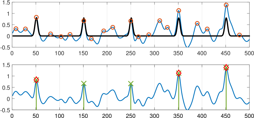
We study the classical problem of detecting the locations of multiple signal occurrences in a noisy measurement. Figure 1 illustrates an instance of the problem, where the goal is to estimate the locations of five signal occurrences from the noisy observation. This detection problem is an essential step in a wide variety of applications, including single-particle cryo-electron microscopy [10, 17], neuroimaging brain mapping [19], microscopy [9, 11], astronomy [5] and retina study [1].
Assuming the shape of the signal is approximately known, the most popular heuristic to detect signal occurrences is correlating the noisy measurement with the signal, and choosing the peaks of the correlation as the estimates of the signals’ locations. If the signal is known, then this method is referred to as a matched filter [15]. However, extending the matched filter to multiple signal occurrences is not trivial, and may lead to high false-alarm rates. This mostly manifests in high noise levels, and in cases where the signal occurrences are densely packed [21].
Following the work of Schwartzman et al. [18, 6], we study the signal detection problem from the perspective of multiple hypothesis testing. In particular, Schwartzman et al. [18] proposed to choose the local maxima of the measurement, after it was correlated with a template which ideally resembles the underlying signal, as the estimators of the locations of the signal occurrences. While this procedure is akin to matched filter, the main contribution of [18] is setting the threshold of the detection problem based on the Benjamini-Hochberg procedure [4] to control the false discovery rate under a desired level. In Section II we introduce the results of [18] in detail. Notably, the statistical test of Schwartzman et al. exploits only local maxima, while ignoring their local neighborhoods. Hereafter, we refer to this scheme as a one-sample statistical test.
In this work, we extend the one-sample statistical test of [18] to account for the neighborhood of the local maxima. In particular, we claim that taking the neighborhood of the local maxima, or its shape, may strengthen the statistical test. For example, if the noise is highly correlated, a narrow and sharp peak is more likely to indicate on a signal occurrence than a wider peak. The first contribution of this paper is extending the framework of [18] to a statistical test which is based on multiple samples around each local maxima; we refer to this procedure as the -sample statistical test. This entails calculating the joint probability distribution of the chosen samples and deriving the corresponding p-value required for the Benjamini-Hochberg procedure.
The second contribution of this work is implementing the new framework for two-sample test (), namely, when the statistical test relies on the local maxima and one additional point in their vicinity. As discussed in Section III, the computational complexity of the K-sample test grows exponentially fast with , and thus we leave the implementation of the -sample test with for future work. We conduct comprehensive numerical experiments, and show that the two-sample test outperforms the one-sample test of [18] in a wide range of scenarios. Figure 1 illustrates a simple example when our two-sample test outperforms the one-sample test of [18].
The rest of the paper is organized as follows. Section II provides mathematical and statistical background. Section III presents the main result of this paper. Section IV discusses computational considerations and presents numerical results. Section V concludes the paper and delineates future research directions.
II Mathematical model and background
Let be a continuous signal with a compact support of unknown location and . Let
| (1) |
be a train of unknown signals, where . Our goal is to estimate the locations of the signals from a noisy measurement of the form
| (2) |
where denotes the noise.
In our problem, the null hypothesis is that there are no signals, namely, a pure noise measurement . This problem can be thought of as a special case of multiple hypothesis testing [16], where our hypothesizes are the points at which we suspect the signal occurrences are located.
II-A Multiple hypothesis testing
In a classical (single) hypothesis testing problem, one considers two hypotheses (the null and the alternative) and decides whether the data at hand sufficiently support the null. Specifically, given a set of observations (e.g., coin tosses), our goal is to increase the probability of making a true discovery (e.g., declare that a coin is biased given that it is truly biased), while maintaining a prescribed level of type I error, (declaring that a coin is biased given that it is not). This is typically done by examining the p-value: the probability of obtaining test results at least as extreme as the result actually observed, under the assumption that the null hypothesis is correct. Specifically, we declare a discovery if the p-value is not greater than .
Multiple testing arises when a statistical analysis involves multiple simultaneous tests, each of which has a potential to produce a ”discovery”. A stated confidence level generally applies only to each test considered individually, but often it is desirable to have a confidence level for the whole family of simultaneous tests. Failure to compensate for multiple comparisons may produce severe consequences. For example, consider a set of coins, where our goal is to detect biased coins. Assume we test the hypothesis that a coin is biased with a confidence level of . Further, assume that all the coins are in-fact unbiased. Then, we expect to make false discoveries. Further, and perhaps more importantly, the probability that we make at least one false discovery (denoted family wise error rate, FWER) increases as grows. This means we are very likely to report that there is at least one biased coin in hand, even if they are all fair. A classical approach for the multiple testing problem is to control the FWER. This is done by applying the Bonferroni correction: it can be shown that by performing each test in a confidence level of , we are guaranteed to have a FWER not greater than . The Bonferroni correction is very intuitive and simple to apply. Yet, it is also very conservative and thus very few discoveries are likely to be made.
To overcome these caveats, Benjamini and Hochberg [4] proposed an alternative criterion. Instead of controlling the FWER, they suggested controlling the false discovery rate (FDR). The FDR is formally defined as the expected proportion of false discoveries from all the discoveries that are made. Thus, we allow more false discoveries if we make more discoveries.
Definition 1.
The false discovery rate (FDR) is defined by
| (3) |
where and are, respectively, the number of false positives and all positives (rejections of null hypothesis).
This criterion is evidently less conservative than the FWER. Thus, FDR-controlling procedures have greater power, at the cost of increased numbers of type I errors. Benjamini and Hochberg introduced a simple approach for controlling the FDR [4]. Their approach is based on sorting the p-values in ascending order . For a desired level , the Benjamini–Hochberg procedure suggests finding the largest such that and reject null hypothesis for all observations of equal or less p-value. The Benjamini-Hochberg procedure made a tremendous impact on modern statistical inference [3], with many important applications to biology [14], genetics [13, 20], bioinformatics [12], statistical learning [8], to name but a few.
II-B Controlling the FDR of local maxima
Going back to our problem, we aim to control the FDR of estimating the locations of the signal occurrences from the measurement . A direct approach is testing on every sampled point in the measurement [19]. However, this approach overlooks the spatial structure of the signals, and correlations in the measurement. In [18], Schwartzman, Gavrilov and Adler developed a method to control the FDR, while testing only the local maxima of a smoothed version of the measurement. Specifically, the algorithm of [18] begins with correlating the measurement with a smoothing kernel of compact connected support satisfying . This results in
| (4) |
where and denote the smoothed signal train and noise, respectively. The next step is finding the set of all local maxima of the smoothed measurement:
| (5) |
To apply the Benjamini-Hochberg procedure, we next need to compute the p-value of each local maxima with respect to the null hypothesis . The p-value is given by
| (6) |
This distribution, describing the probability of local maxima of , is called the Palm distribution [7, Chapter 11], and is given by the following CDF:
| (7) |
where and are the normal density and its CDF respectively, while , and are the first three moments of .
Finally, we apply the Benjamini–Hochberg procedure, to control the FDR at a desired level . The algorithm of Schwartzman et al., dubbed one-sample test, is summarized in Algorithm 1. Interestingly, it was shown that this procedure achieves maximal power under asymptotic conditions [18].
III Main Result
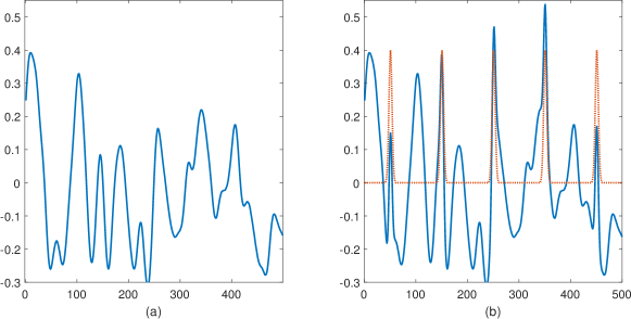
Careful examination of local maxima reveals that not all peaks of the same height are also of a similar shape: the existence of a signal occurrence underneath the noise varies the general shape of the local maximum; see Figure 2 for an example. Accordingly, we suggest taking into account the vicinity of the local maxima in the estimation process. In this section, we provide an explicit expression of the joint distribution of the local maximum and its closely-located samples. This in turn allows us to calculate the corresponding p-value which can be used to control the FDR using the Benjamini-Hochberg procedure.
Let be the maximum of a random Gaussian vector . We assume that consists of no more then a single local maximum. Our goal is to evaluate the joint distribution of and its neighbors, ordered in an arbitrary manner ,
| (8) |
Applying the chain rule, we have
| (9) | ||||
The one-dimensional distribution of a local maxima , or Palm distribution as mentioned earlier, was derived in [7]. Therefore, the following result allows us to evaluate the joint distribution (8).
Proposition 1.
Let be the maximum of a multivariate Gaussian vector . Let be an arbitrary order of points other than . Define
and
Then, for any , we have:
where is the cumulative distribution function (CDF) of and is an indicator function.
Proof.
Using Bayes’ Theorem, we have:
| (10) | |||
The denominator satisfies
while the numerator
∎
Equipped with the explicit expression of the joint distribution of the local maximum and its neighbors, we are ready to define the corresponding p-value. The p-value is essential in order to apply the Benjamini-Hochberg procedure. In this work the p-value at is defined by:
| (11) |
We emphasize that alternative definitions of p-value may be used, and we chose the conservative (11) to mitigate the computational complexity, which is the focus of the next section. Our proposed scheme is summarized in Algorithm 2.
IV Numerical experiments
Computing the p-value corresponding to (8) is computationally demanding as one needs to evaluate multi-dimensional integrals. In particular, the computational burden grows quickly with : the number of samples we consider around each local maximum. Therefore, we implemented our algorithm for a single neighbor (namely, ) at a distance from the local maxima; we refer to this algorithm as a two-sample test. In addition, to mitigate the computational burden, we approximate the marginal distribution as a truncated Gaussian distribution. This is only an approximation that we used to alleviate the computational load since the marginal of a truncated Gaussian distribution is not necessarily a truncated Gaussian distribution. Nevertheless, we found empirically that this approximation provides good numerical results.
We compared Algorithm 2 with with the one-sample test of [18], Algorithm 1. We set the length of the measurement to , with 10 truncated Gaussian signals
| (12) |
with . The parameter , the standard deviation of the Gaussian, controls the width of the signal, and has a significant influence on the performance of the algorithms. Following [18], we generated the noise with parameter according to where is Brownian motion and is a noise parameter. Notice that this noise is a convolution of white Gaussian noise of zero mean and variance with a CDF of Gaussian with zero mean and variance . The latter can be seen as a parameter governing the noise correlation level. This specific noise distribution was chosen because of available good approximations of its three first moments: , and . Those approximations will be useful in calculating p-values according to (7). The smoothing kernel is chosen to be with varying values of . We set the FDR level to be .
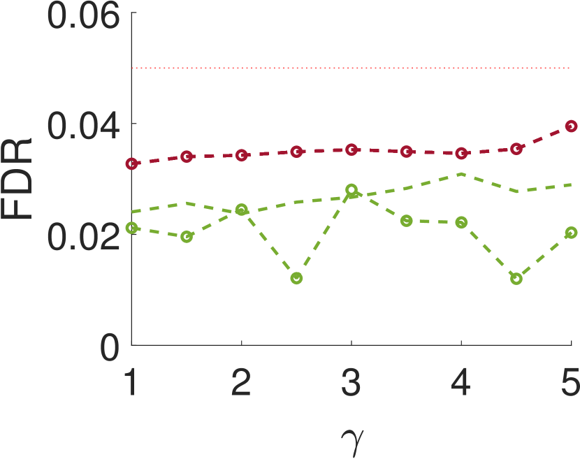
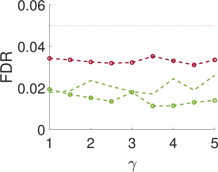
Following [18], we define a true positive to be any estimator inside the support of a true signal occurrence. Similarly, a false positive is an estimator outside the support of any true signal occurrence. We compare the algorithms for different values of (the variance of the Gaussian used to generate a correlated noise), (the variance of the Gaussian signal), and (the variance of the Gaussian smoothing kernel). For each set of parameters, we present the average power and false discovery rate, averaged over 1000 trials.
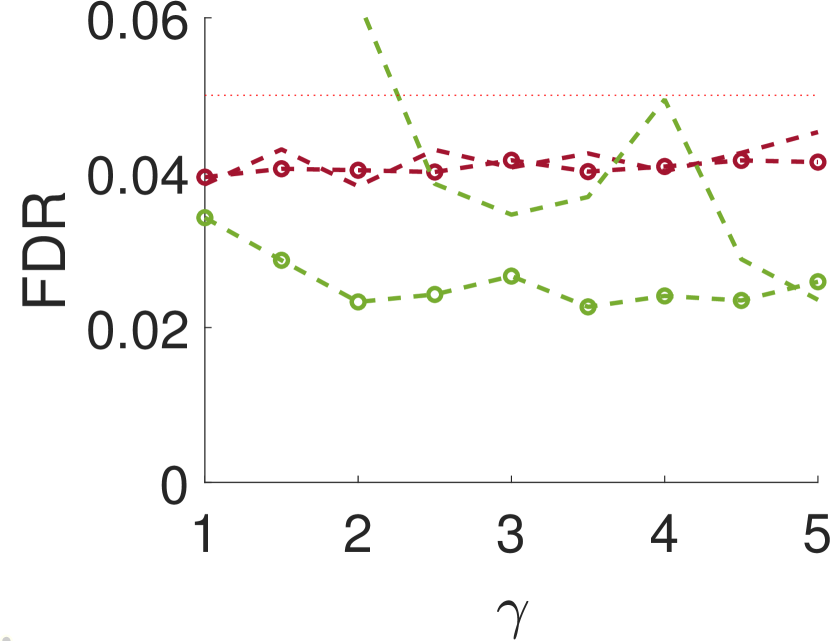
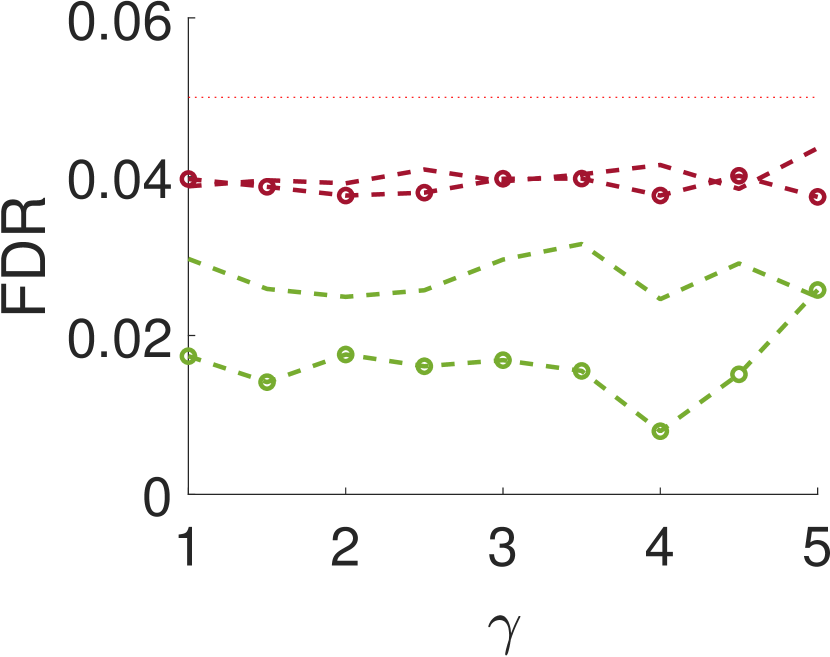
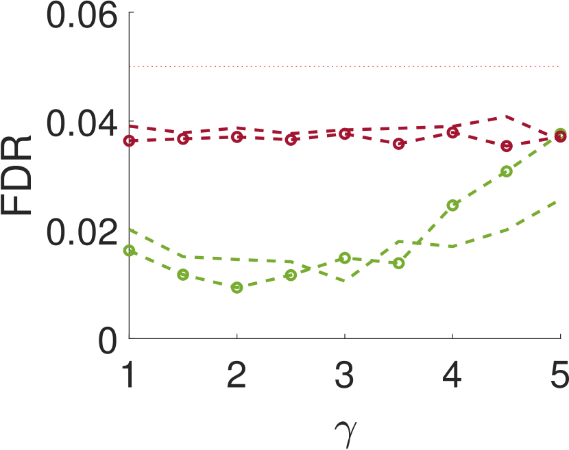
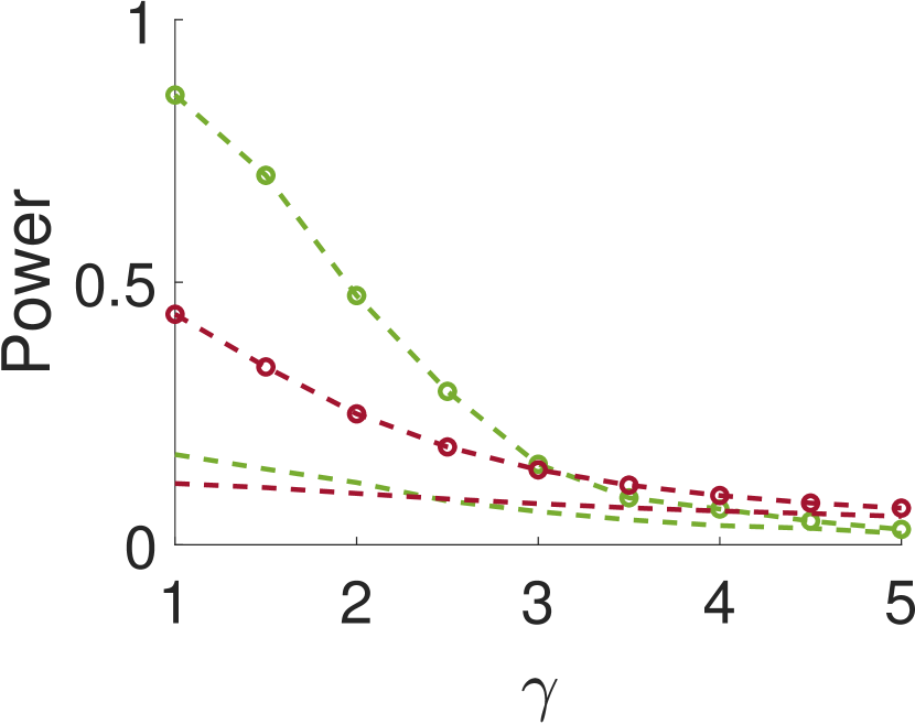
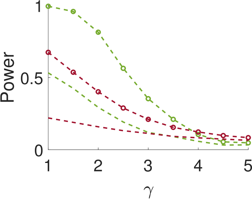
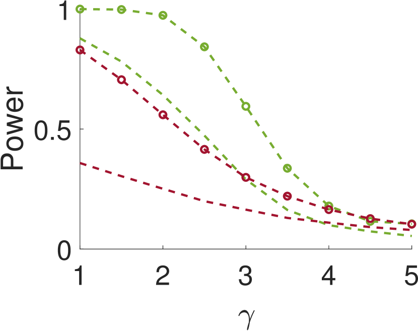
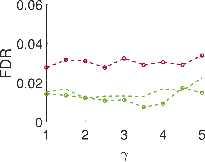
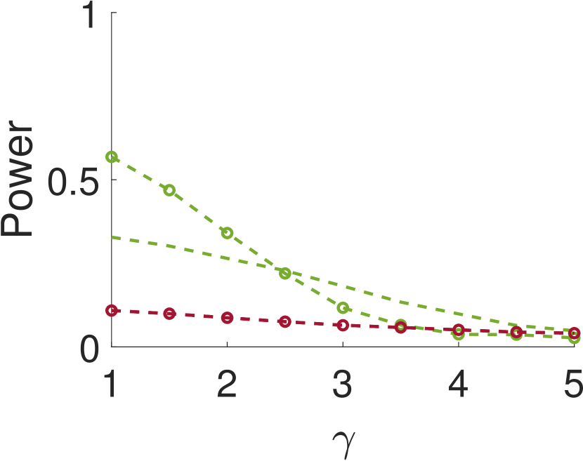
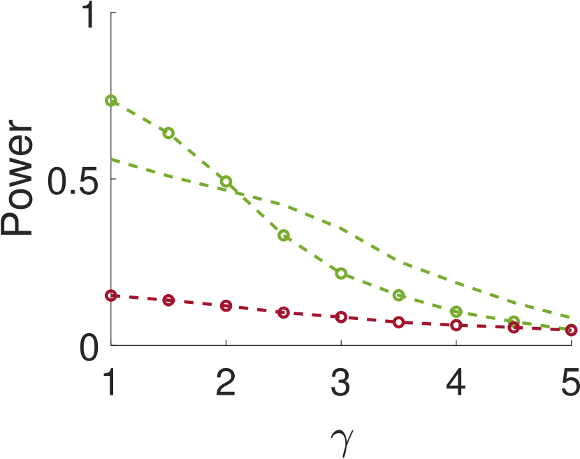
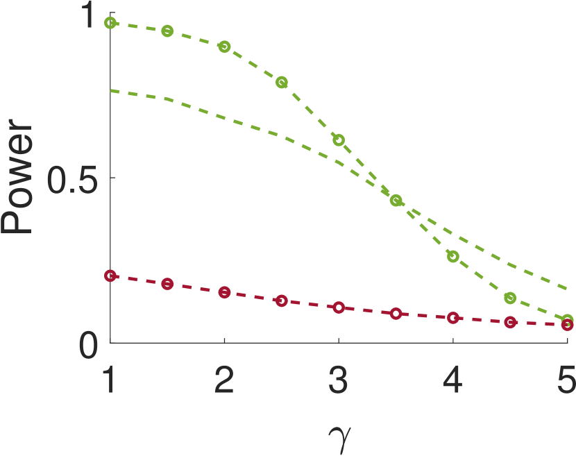
Figure 3 shows the power and FDR of Algorithms 1 and 2, for a range of values for the parameters and with a neighbor at distance of (for Algorithm 2). While both tests control the FDR below almost everywhere, the power of the two-sample test is clearly greater than the power of the one-sample test. The gap increases for smaller values of , namely, for narrower signals. This phenomenon can be explained as for wider signals the adjacent samples are similar to the local maxima; in the extreme, it can be thought of as sampling twice the same local maximum.
We repeat the same experiment with , and the results are presented in Figure 4. As can be seen, the results for large are quite similar to the case of . However, for small values of , when the noise is weakly correlated, the power is clearly inferior. This happens since, in this case, a sample entries away from the local maximum does not provide much information on the local maximum itself.
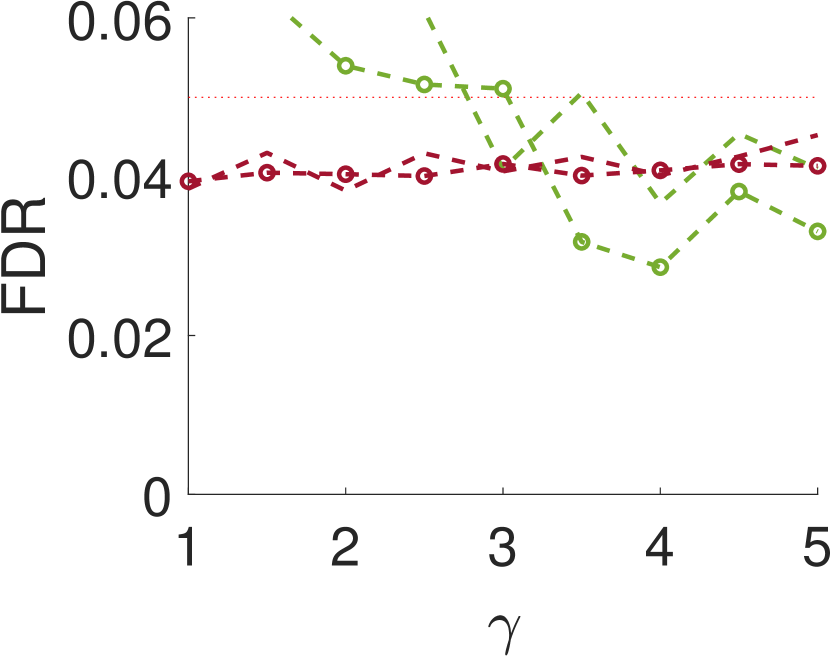
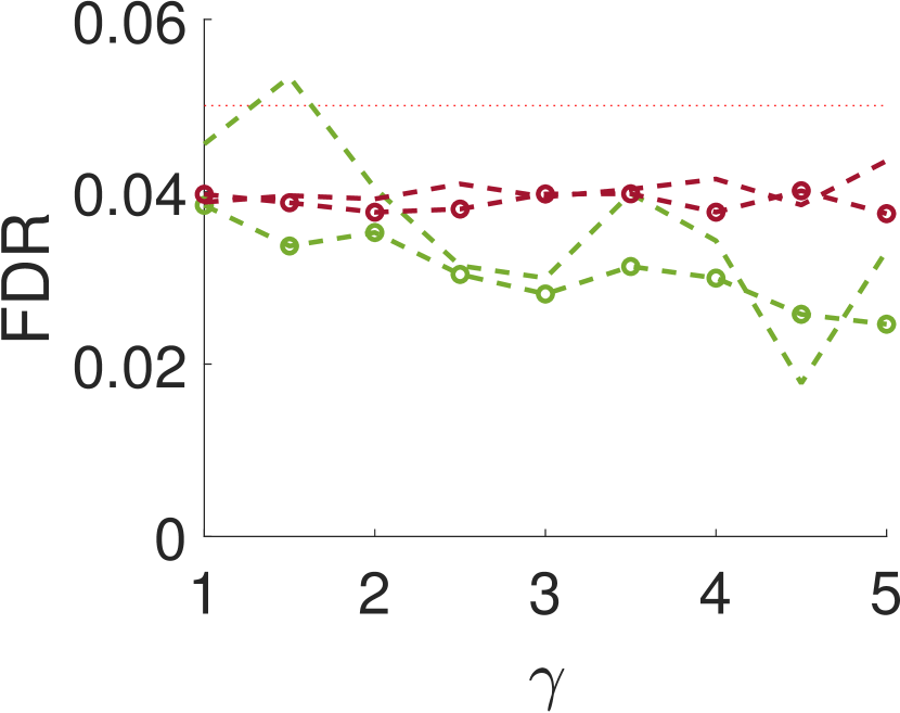
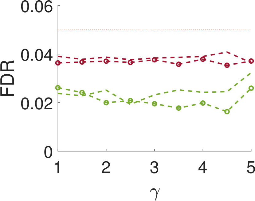
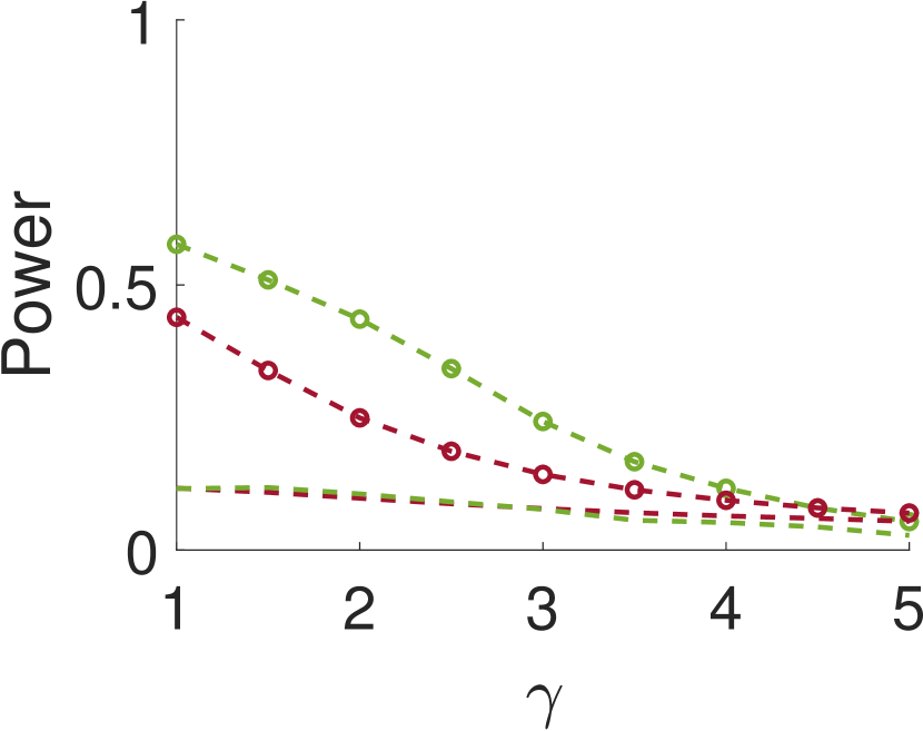
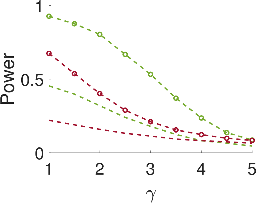
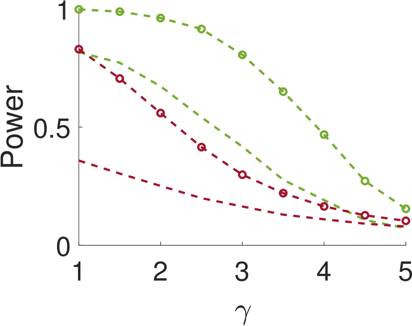
Figure 5 compares Algorithm 2 for and . For all values of , the case of outperforms for small values of (the parameter of the smoothing kernel). For large , on the other hand, the latter outperforms the former. This happens since large implies smoother noise and thus examining samples farther away from the local maxima provides more information.
V Conclusions and discusssion
This paper introduces a new statistical test for detecting signal occurrences in a noisy measurement that controls the FDR below a desired level. In particular, our procedure does not only consider the local maxima of the measurement, but also its neighbors. We numerically show that our two-sample test outperforms the one-sample test of [18] for correlated noise (large enough ). In particular, it seems that for about twice the variance of the signal and neighboring distance of around , our algorithm yields good performance. The FDR of our algorithm is usually lower than the FDR of the one-sample test, probably due to the conservative p-value definition (11).
The main impediment of the proposed procedure is evaluating the multi-dimensional integrals (III), limiting the current implementation to a two-sample test. We aim to extend this work to a -sample test with . To this end, we intend to examine different approximation schemes of the integrals, perhaps along the lines of the truncated Gaussian approximation we use in this work. We expect that such extension will significantly improve the performance of the algorithm. Another future work is to follow the blueprint of [6] and extend our -sample test to images. This might be particularly important for the particle picking task: an essential step in the computational pipeline of single-particle cryo-electron microscopy [2].
References
- [1] Stephen A Baccus and Markus Meister. Fast and slow contrast adaptation in retinal circuitry. Neuron, 36(5):909–919, 2002.
- [2] Tamir Bendory, Alberto Bartesaghi, and Amit Singer. Single-particle cryo-electron microscopy: Mathematical theory, computational challenges, and opportunities. IEEE Signal Processing Magazine, 37(2):58–76, 2020.
- [3] Yoav Benjamini. Simultaneous and selective inference: Current successes and future challenges. Biometrical Journal, 52(6):708–721, 2010.
- [4] Yoav Benjamini and Yosef Hochberg. Controlling the false discovery rate: a practical and powerful approach to multiple testing. Journal of the Royal statistical society: series B (Methodological), 57(1):289–300, 1995.
- [5] Pierpaulo Brutti, Christopher Genovese, Christopher J Miller, Robert C Nichol, and Larry Wasserman. Spike hunting in galaxy spectra. 2005.
- [6] Dan Cheng and Armin Schwartzman. Multiple testing of local maxima for detection of peaks in random fields. Annals of statistics, 45(2):529, 2017.
- [7] Harald Cramér and M Ross Leadbetter. Stationary and related stochastic processes: Sample function properties and their applications. Courier Corporation, 2013.
- [8] Bradley Efron, Trevor Hastie, Iain Johnstone, and Robert Tibshirani. Least angle regression. The Annals of statistics, 32(2):407–499, 2004.
- [9] Alexander Egner, Claudia Geisler, Claas Von Middendorff, Hannes Bock, Dirk Wenzel, Rebecca Medda, Martin Andresen, Andre C Stiel, Stefan Jakobs, Christian Eggeling, et al. Fluorescence nanoscopy in whole cells by asynchronous localization of photoswitching emitters. Biophysical journal, 93(9):3285–3290, 2007.
- [10] Joachim Frank. Three-dimensional electron microscopy of macromolecular assemblies: visualization of biological molecules in their native state. Oxford university press, 2006.
- [11] Claudia Geisler, Andreas Schönle, C Von Middendorff, Hannes Bock, Christian Eggeling, Alexander Egner, and SW Hell. Resolution of /10 in fluorescence microscopy using fast single molecule photo-switching. Applied Physics A, 88(2):223–226, 2007.
- [12] Da Wei Huang, Brad T Sherman, and Richard A Lempicki. Bioinformatics enrichment tools: paths toward the comprehensive functional analysis of large gene lists. Nucleic acids research, 37(1):1–13, 2009.
- [13] Michael I Love, Wolfgang Huber, and Simon Anders. Moderated estimation of fold change and dispersion for RNA-seq data with DESeq2. Genome biology, 15(12):1–21, 2014.
- [14] John H McDonald. Handbook of biological statistics, volume 2. sparky house publishing Baltimore, MD, 2009.
- [15] William K Pratt. Digital image processing: PIKS Scientific inside, volume 4. Wiley Online Library, 2007.
- [16] G Rupert Jr et al. Simultaneous statistical inference. 2012.
- [17] Sjors HW Scheres. RELION: implementation of a Bayesian approach to cryo-EM structure determination. Journal of structural biology, 180(3):519–530, 2012.
- [18] Armin Schwartzman, Yulia Gavrilov, and Robert J Adler. Multiple testing of local maxima for detection of peaks in 1D. Annals of statistics, 39(6):3290, 2011.
- [19] Jonathan E Taylor and Keith J Worsley. Detecting sparse signals in random fields, with an application to brain mapping. Journal of the American Statistical Association, 102(479):913–928, 2007.
- [20] Virginia Goss Tusher, Robert Tibshirani, and Gilbert Chu. Significance analysis of microarrays applied to the ionizing radiation response. Proceedings of the National Academy of Sciences, 98(9):5116–5121, 2001.
- [21] Vio, R., Andreani, P., Biggs, A., and Hayatsu, N. The correct estimate of the probability of false detection of the matched filter in weak-signal detection problems - iii. peak distribution method versus the gumbel distribution method. A&A, 627:A103, 2019.