K-Shell Photoabsorption of Magnesium Ions

M. F. Hasoğlu Department of Computer Engineering, Hasan Kalyoncu University, 27100 Sahinbey, Gaziantep, Turkey Sh. A. Abdel-Naby Department of Physics, Auburn University, Auburn, Alabama 36849, USA E. Gatuzz Centro de Física, Instituto Venezolano de Investigaciones Científicas, Caracas 1020, Venezuela J. García Harvard-Smithsonian Center for Astrophysics, MS-6, 60 Garden Street, Cambridge, MA 02138, USA T. R. Kallman NASA Goddard Space Flight Center, Greenbelt, MD 20771, USA C. Mendoza Department of Physics, Western Michigan University, Kalamazoo, MI 49008-5252, and Centro de Física, Instituto Venezolano de Investigaciones Científicas, Caracas 1020, Venezuela T. W. Gorczyca Department of Physics, Western Michigan University, Kalamazoo, MI 49008-5252, USA

Abstract

X-ray photoabsorption cross sections have been computed for all magnesium ions using the $R$ -matrix method. A comparison with the other available data for Mg II–Mg X shows good qualitative agreement in the resultant resonance shapes. However, for the lower ionization stages, and for singly-ionized Mg II in particular, the previous $R$ -matrix results (Witthoeft et al., 2009; Witthoeft et al., 2011) overestimate the K-edge position due to the neglect of important orbital relaxation effects, and a global shift downward in photon energy of those cross sections is therefore warranted. We have found that the cross sections for Mg I and Mg II are further complicated by the M-shell ( $n=3$ ) occupancy. As a result, the treatment of spectator Auger decay of $1s\rightarrow np$ resonances using a method based on multichannel quantum defect theory and an optical potential becomes problematic, making it necessary to implement an alternative, approximate treatment of Auger decay for neutral Mg I. The new cross sections are used to fit the Mg K edge in XMM-Newton spectra of the low-mass X-ray binary GS 1826-238, where most of the interstellar Mg is found to be in ionized form.

atomic processes — atomic data — line: formation — ISM: abundances

^†^†slugcomment: Not to appear in Nonlearned J., 45.

1 Introduction

Accurate K-shell photoabsorption cross sections are necessary for modeling astrophysical plasmas, interpreting the observed spectra from distant cosmic emitters, and determining the elemental abundances of the interstellar medium (ISM). Spectra of K-shell processes can be observed from all ionic stages of the most abundant elements between oxygen and nickel (Paerels & Kahn, 2003). Magnesium K lines, in particular, have been observed since the early days of X-ray astronomy; for instance, in the spectrum of the O4 $\zeta$ Puppis star taken with the Broad-Band X-Ray Telescope associated with a thermal plasma of $\sim 6\times 10^{6}$ K (Corcoran et al., 1993). These findings were used, in spite of observational shortcomings such as short exposure times, to constrain the location, temperature, and chemical abundances of the emitting region.

With the advent of high-resolution satellite-borne observatories such as Chandra, XMM-Newton, and Suzaku, X-ray spectroscopy has come of age to provide unique opportunities for studying in detail the physical conditions and processes of exotic and energetic sources. Such is the case of emission K lines from hydrogen-, helium-, and lithium-like Mg ions observed in the supernova remnant N132D (Behar et al., 2001); the active nucleus of the giant elliptical galaxy M 87 (Sakelliou et al., 2002); the massive X-ray binary Cen X-3, where the importance of resonant line scattering in photoionized plasmas was highlighted (Wojdowski et al., 2003); the accretion disk of the low-mass X-ray binary system EXO 0748-676 providing evidence of a neutron star (Jimenez-Garate et al., 2003); the Seyfert 2 galaxy Mkn 3 (Pounds & Page, 2005); the outflow component of quasar PG 1211+143 (Kaspi & Behar, 2006); the Cap region above the disk of the starburst galaxy M82, where metal abundance ratios are consistent with Type-II supernova nucleosynthesis (Tsuru et al., 2007); the Fornax intracluster medium allowing an accurate measurement of the Mg abundance that leads to an estimate of the ratio $[{\rm Mg/Fe}]\approx 0.5{-}0.7$ that reflects a stellar metalicity (Matsushita et al., 2007); the highly variable narrow-line Seyfert Type 1 galaxy NGC 4051 giving outflow velocities of $\sim 600$ km s^-1 (Lobban et al., 2011); and the Galactic supernova remnant G346.6-0.2 that suggests ejecta-dominated emission with relative abundances pointing to a Type Ia supernova explosion (Sezer et al., 2011). Yamaguchi et al. (2012) have recently studied the spectrum of the Galactic supernova remnant G344.7–0.1, detecting for the first time in an extended celestial source the K $\alpha$ line from Al XII at $\sim 1.6$ keV. This is an important finding because, since both Mg and Al are synthesized during C/Ne burning, the Al/Mg abundance ratio would be a sensitive metalicity diagnostic. This indicator is currently limited by both spectral resolution, which will be improved in the near future with the launching of the Astro-H telescope, and atomic data.

Absorption Mg K lines are also observed in ISM spectra towards X-ray sources where a desirable feature would be to determine the amount of this element locked up in grain minerals. Pinto et al. (2010) have measured the spectrum of the low-mass X-ray binary GS 1826-238, finding a Mg abundance of $2.45\pm 0.35$ solar that appears to be consistent with a proposed Galactic gradient. Also, the ultra-compact binary candidate 4U0614+091 observed by Schulz et al. (2010) shows a strong variability that causes an excess component intrinsic to the source that demands adjustments of the Ne edge; however, an excess in the Mg edge is not as yet conclusive partly due to its unestablished morphology.

In previous studies, we have carried out accurate calculations of K-shell photoabsorption cross sections that have been applied to X-ray spectral diagnostics; e.g. all ionization stages of carbon (Hasoğlu et al., 2010), oxygen (Gorczyca & McLaughlin, 2000; García et al., 2005; Juett et al., 2004), and neon (Gorczyca, 2000; Juett et al., 2006). This project is hereby extended to the magnesium isonuclear sequence where a further complication arises for the two lowest ionization stages (Mg I and Mg II) as the $n=3$ M-shell becomes occupied: the atomic radius now doubles in size, and our usual treatment based on multichannel quantum defect theory (MQDT) and an optical potential (Gorczyca & Robicheaux, 1999) becomes problematic for the lower $1s\rightarrow np$ resonances. We have nevertheless come up with an approximate procedure for treating these cases that yields reliable X-ray photoabsorption cross sections for all relevant magnesium ions, i.e. Mg I–Mg X. Furthermore, these new cross sections will allow us to revise the Mg abundance in the low-mass X-ray binary GS 1826-238 and, in particular, to determine the ionic fractions, if any, of the lowly ionized species.

2 Theoretical Approach

K-shell photoabsorption consists of the direct photoionization of the $1s$ electron, which is treated in a straightforward manner using $R$ -matrix methods, and the strong $1s\rightarrow np$ photoabsorption resonances. Photoexcitation of these resonance states is then followed by two competing decay routes. The first is participator Auger decay, where the $np$ valence electron takes part in the autoionization process with a decay rate that scales as $1/n^{3}$ and goes to zero near the K-shell threshold. These channels are included in the $R$ -matrix calculation. The second route is spectator Auger decay, in which $np$ the valence electron is oblivious to the autoionization process giving instead a decay width that is independent of $n$ . Therefore, the latter is the dominant decay route as $n\rightarrow\infty$ , and guarantees a smooth cross section as the K-shell threshold is approached. Above threshold, K-shell photoionization to the $1s2\ell^{q}$ states occurs instead.

For the present work we use the $R$ -matrix method (Berrington et al., 1995; Burke, 2011) with modifications to account for the spectator Auger broadening via an optical potential as described by Gorczyca & Robicheaux (1999). This enhanced $R$ -matrix method has been shown to be accurate in describing experimental synchrotron measurements for argon (Gorczyca & Robicheaux, 1999), oxygen (Gorczyca & McLaughlin, 2000), neon (Gorczyca, 2000), and carbon (Hasoğlu et al., 2010). The Auger widths for the $1s2\ell^{q}$ states are computed by applying the Smith (1960) time-delay method to the photoabsorption $R$ -matrix calculation of the neighboring $1s^{2}2\ell^{q-1}$ magnesium ion. Further details can be found in our previous work (Gorczyca & Robicheaux, 1999; Gorczyca & McLaughlin, 2000; Gorczyca, 2000; Hasoğlu et al., 2010).

3 Cross Section Results

As an assessment of the present atomic description, the computed target-state energies and binding energies are presented in Tables 1–10, which show fairly good agreement with the recommended NIST spectroscopic values. The computed core Auger widths, which are used within the MQDT optical potential approach for treating spectator Auger resonance broadening, are listed in Tables 11–19. Comparison with other available data shows fairly good agreement in most cases, indicating again that the present atomic representations are sufficient. It is worth mentioning that the spectator Auger width used in our calculations only changes the shape of the resonance absorption profile, not the strength.

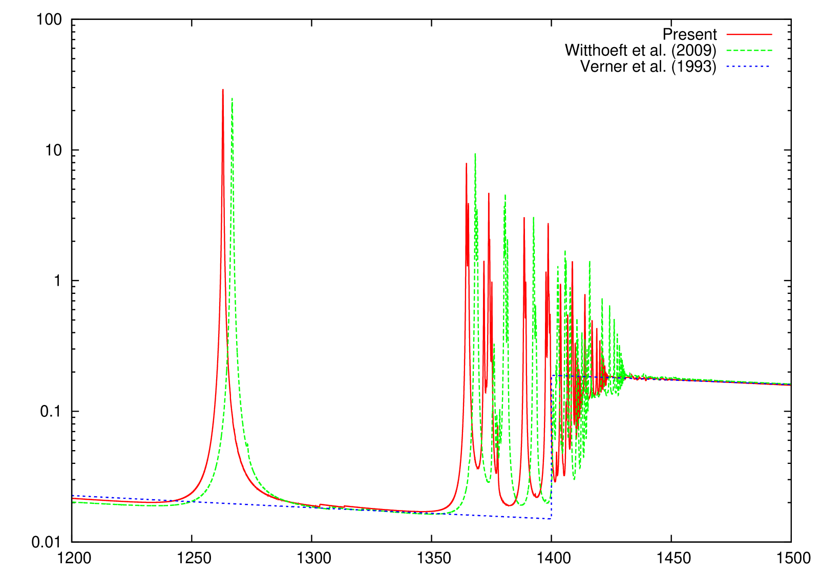
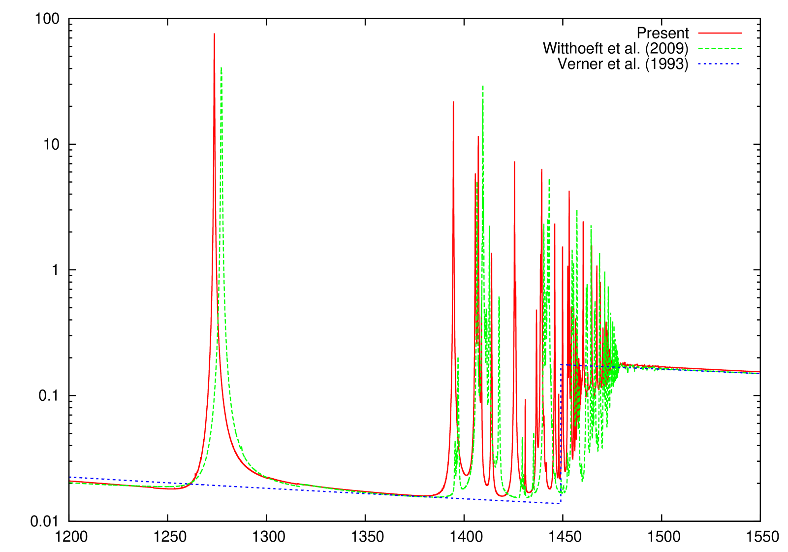
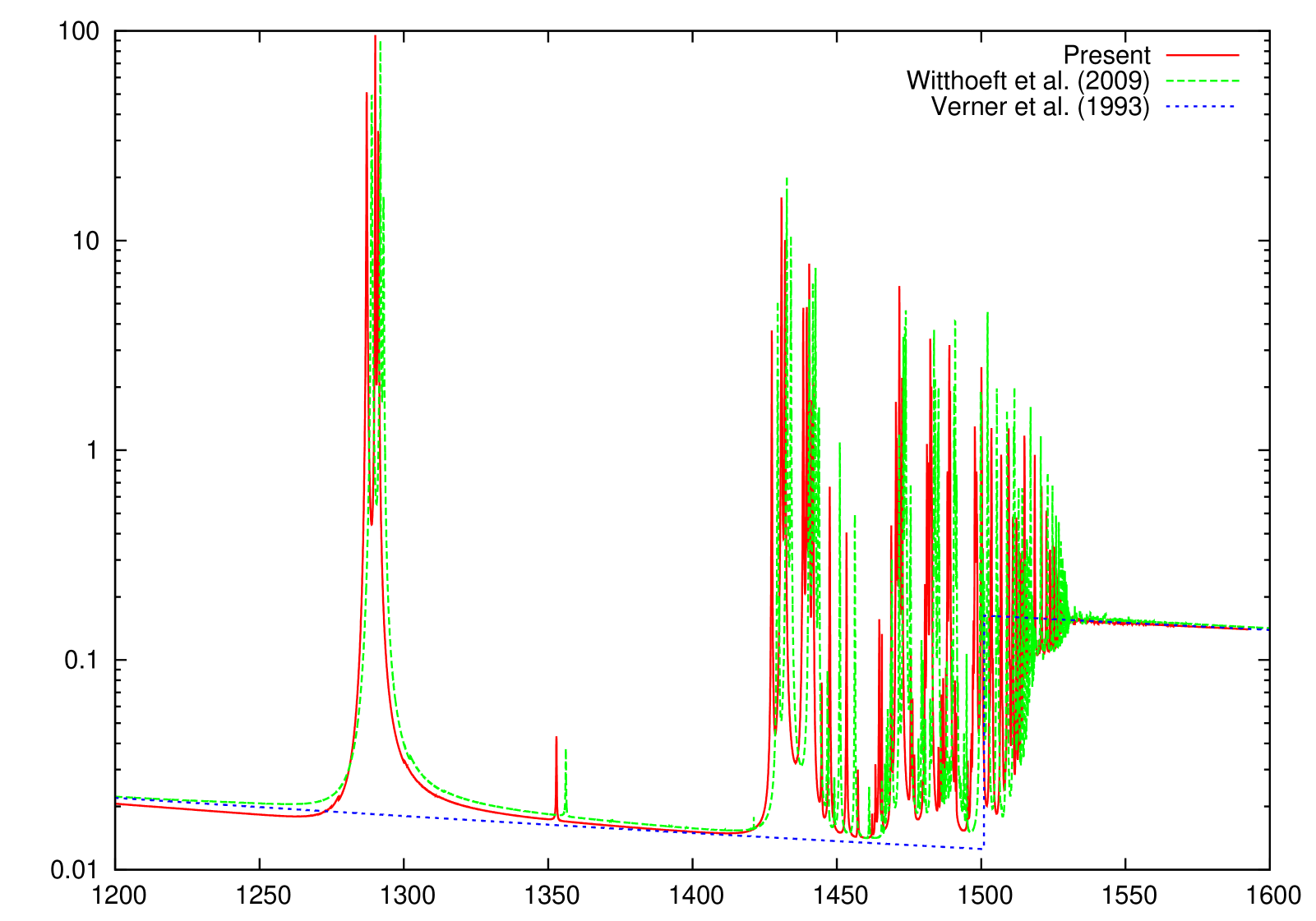
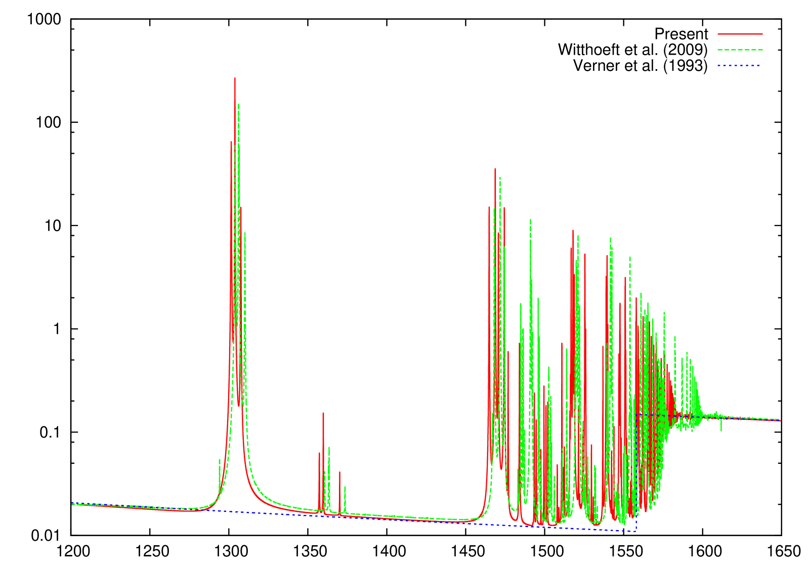
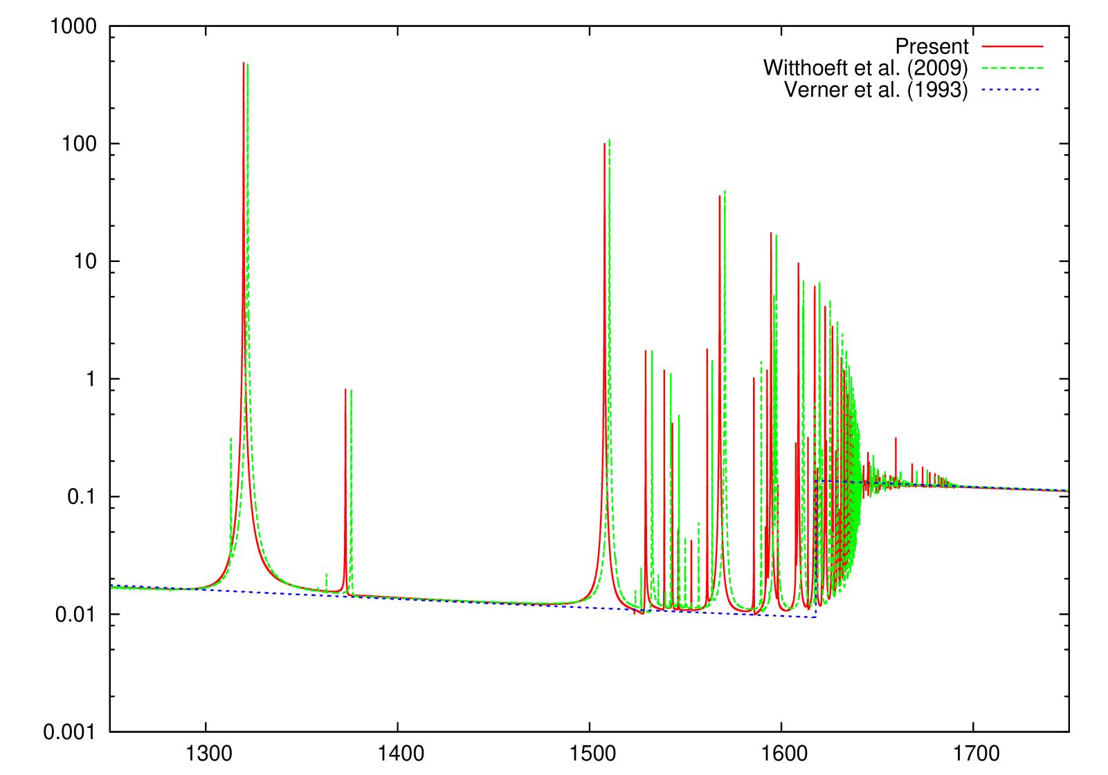
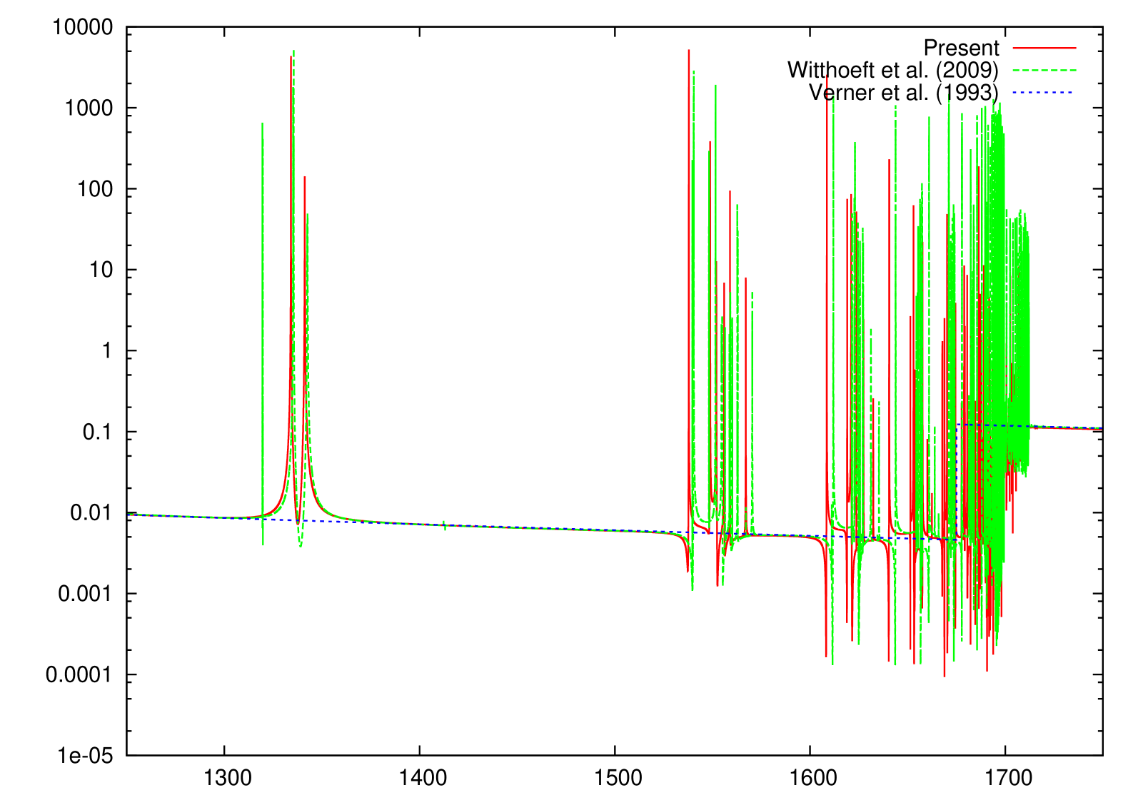
The present K-shell photoabsorption cross sections are shown in Figs. 1–10 where the independent-particle (IP) photoionization results of Verner et al. (1993) are also included. It can be seen that the present $R$ -matrix results are in good quantitative agreement with the IP results above the K-shell thresholds, but the IP cross sections lack the important resonance absorption lines below threshold.

3.1 Neutral Mg

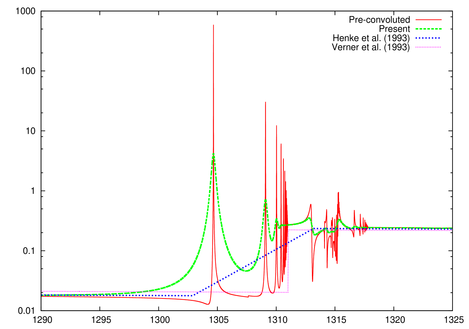
For the Mg I photoabsorption cross section (Fig. 1), there are no other $1s\rightarrow np$ resonance cross sections available for comparison. However, as can be deduced from Table 1, our theoretical K-shell threshold is at 1311.03 eV in fairly good agreement with the experimental value of 1311.4 eV (Banna et al., 1982). Furthermore, since our above-threshold cross section is seen to align with the IP results, we are confident about the below-threshold resonance oscillator strength that merges to the above-threshold oscillator strength density through continuity conditions intrinsic within the $R$ -matrix framework. Also shown in Fig. 1 are the solid-state experimental results of Henke et al. (1993); it is interesting to note that the present $R$ -matrix results for neutral magnesium align more closely with experiment than with the IP results which do not include relaxation effects but shift the threshold downward to align with experiment.

Regarding the $R$ -matrix calculations for Mg I, it was not possible to apply the usual MQDT optical potential method (Gorczyca & Robicheaux, 1999) to render spectator Auger broadening since, due to the larger radius of the $R$ -matrix box (Berrington et al., 1995; Burke, 2011), the energy dependence of the MQDT parameters at the lower resonances invalidated the simple $E\rightarrow E+i\Gamma/2$ substitution (Gorczyca & Robicheaux, 1999). Instead, a more rigorous approach (beyond the scope of this paper) is necessary for the adequate modeling of the Auger width. (As noted before, the strength is not affected by the particular width used.) In order to present reliable cross sections for this study, then, we first perform calculations using a spectator width that is small enough such that the energy-dependent MQDT parameters can still be treated as constant over the width of a resonance, but large enough such that the resonance Rydberg series can be mapped out with a finite number of $R$ -matrix energy points. These cross sections are then further convoluted with a Lorentzian profile of width 0.0254 Ryd (see Table 11) to simulate the known Auger broadening.

3.2 Ionized Mg species

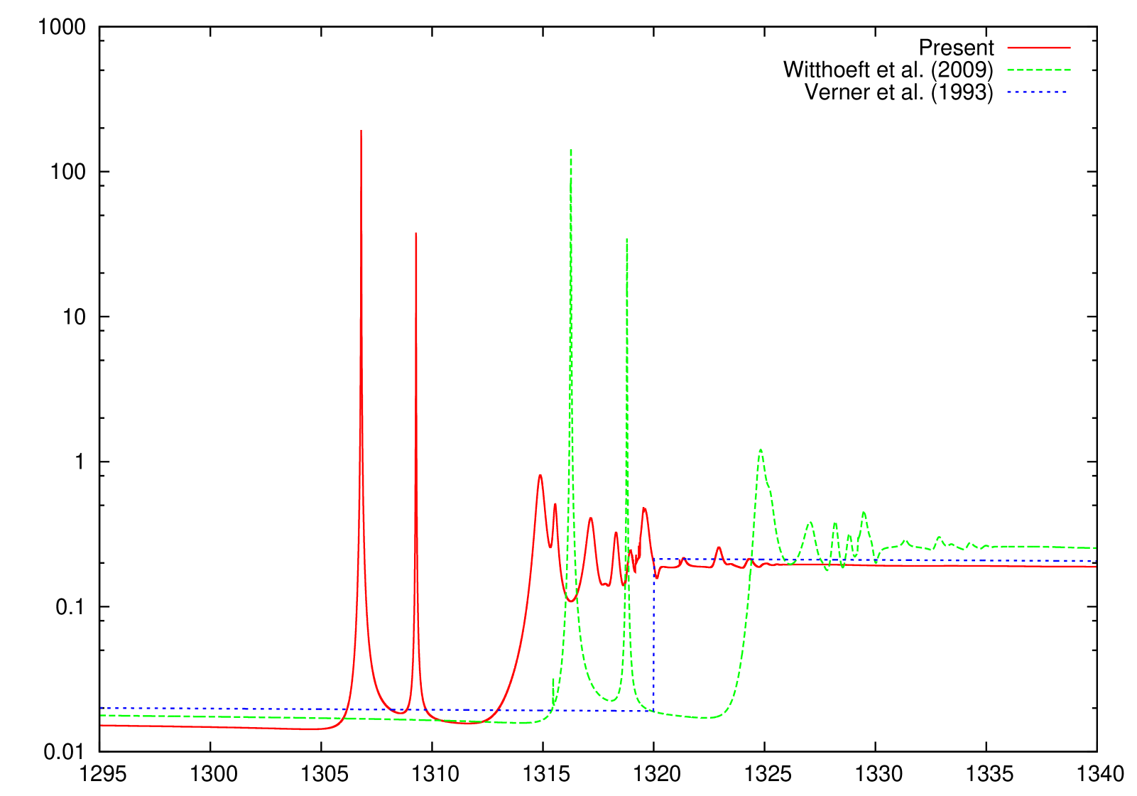
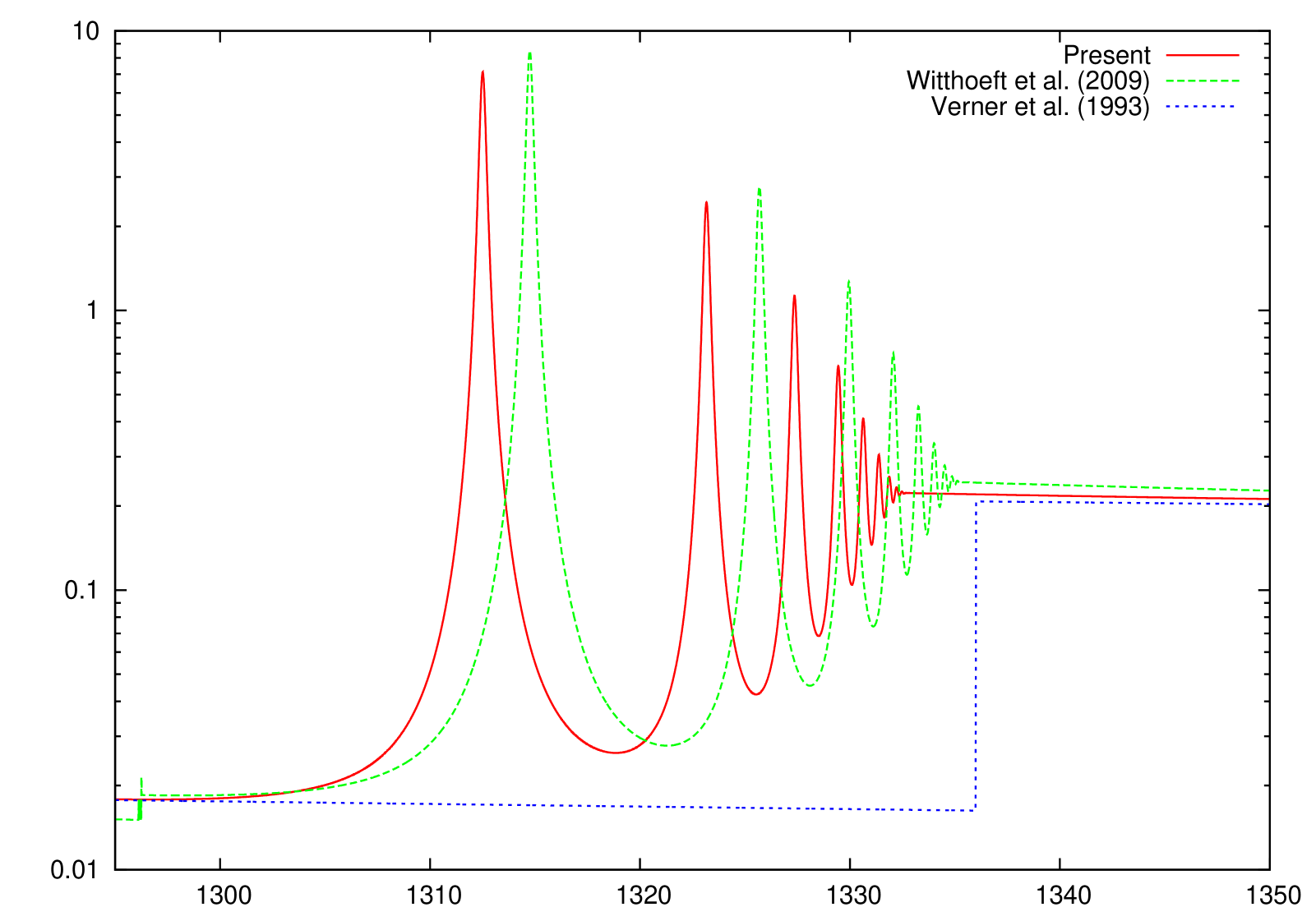
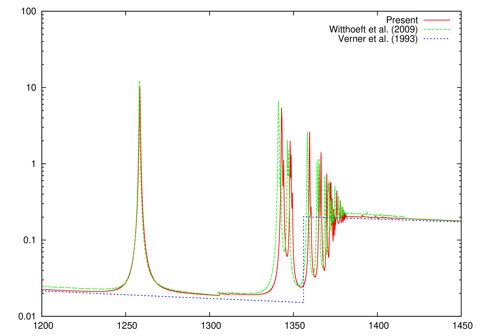
The only other reported K-absorption ( $1s\rightarrow np$ ) cross sections of Mg ionized species, to our knowledge, are those by Witthoeft et al. (2009) and Witthoeft et al. (2011), which have been computed with a similar $R$ -matrix approach; however, important orbital relaxation effects were therein neglected. Relaxation is due to the sudden change in the potential perceived by the outermost electrons following excitation or ionization of an inner-shell electron ( $1s$ electron in this case), the relative change in potential strength reaching a maximum at the lower ionization stages; hence, Mg II is expected to be the most affected by relaxation as evidenced by the K-shell threshold being overestimated by approximately 10 eV. This overestimate, due to the absence of relaxation effects, is seen to diminish as the ionic charge increases to the order of 2 eV, which seems to indicate lack of correlation perhaps from strong $2p^{2}\rightarrow\overline{3d}^{2}$ double promotions that, in addition, would require the inclusion of optimized $\overline{3d}$ pseudo-orbitals.

3.3 Final Atomic Data

Having computed reliable photoabsorption cross sections for Mg I-Mg X in the vicinity of their respective K-edges, we then produced final data sets, to be used in the xstar spectral modeling code (Bautista & Kallman, 2001), by a single fitting formula for each ion, as described more fully in a recent paper on O I (Gorczyca et al., 2013). Briefly, the X-ray photoabsorption cross section for each ion is modeled as a sum of contributions from all possible photoionization mechanisms. For the direct (non-resonant) photoionization cross sections of the $1s$ , $2s$ , $2p$ , and (for Mg I and Mg II) the $3s$ sub-shells, the analytic formulas given by Verner et al. (1993); Verner et al. (1996) are used. However, due to the relatively larger relaxation effects for neutral Mg I, we use instead a three-parameter asymptotic inverse power law fit to the data of Henke et al. (1993) for the $1s$ partial cross section; a similar procedure was done for neutral O I, for reasons discussed at length in that paper (Gorczyca et al., 2013).

While the Verner et al. (1993); Verner et al. (1996) or inverse power formulas yield the direct partial cross sections, the resonant absorption cross sections - predominantly due to the $1s\rightarrow np$ resonances - that contribute to the total cross section are represented by infinite sums of Lorentzian profiles for each Rydberg series. We note also that for the weaker, excited $1s2s^{2}2p^{6}3s3pns$ and $1s2s^{2}2p^{6}3s3pnd$ series in Mg I, as shown above the Mg II $1s2s^{2}2p^{6}3s^{2}$ threshold of 1311 eV in Fig. 1, a modified, asymmetric Fano for the profile is used rather than a Lorentzian fit. This single analytic expression for the total photoabsorption cross section - one for each Mg ion, differing only in the fitting parameters used - ensures a reliable and continuous data set for the entire x-ray region of interest, going well above and well below the Mg K-edge region.

4 Modeling the Mg K edge

We use XMM-Newton spectra from the low-mass X-ray binary GS 1826-238 (Galactic coordinates $l=9.27$ and $b=-6.08$ ) to analyze Mg photoabsorption in the ISM. The data were obtained with the Reflection Grating Spectrometers (RGS) and the reduction process was performed with the XMM-Newton Science Analysis System (SAS, Version 12.0.1). The two observations (see Table 20) are fitted simultaneously in the 8–11 Å wavelength region, the data being rebinned to obtain at least 20 counts per channel in order to use chi-square statistics (Nousek & Shue, 1989). For the analysis we have used the isis (Version 1.6.2-27) package to compare the TBnew and warmabs models to estimate the impact of the new atomic data on ISM indices such as ionization state, relative ionic fractions, and elemental abundances. TBnew is an X-ray absorption model that includes chemical species from H to Ni by implementing the cross sections of Verner et al. (1996) although it only considers photoabsorption in neutrals. On the other hand, warmabs takes into account both the neutral and all ionized species with $Z\leq 30$ , and their relative fractions are determined self-consistently by solving the ionization balance in the gas; moreover, its atomic database is being systematically improved and now includes the Mg photoionization cross sections presented here.

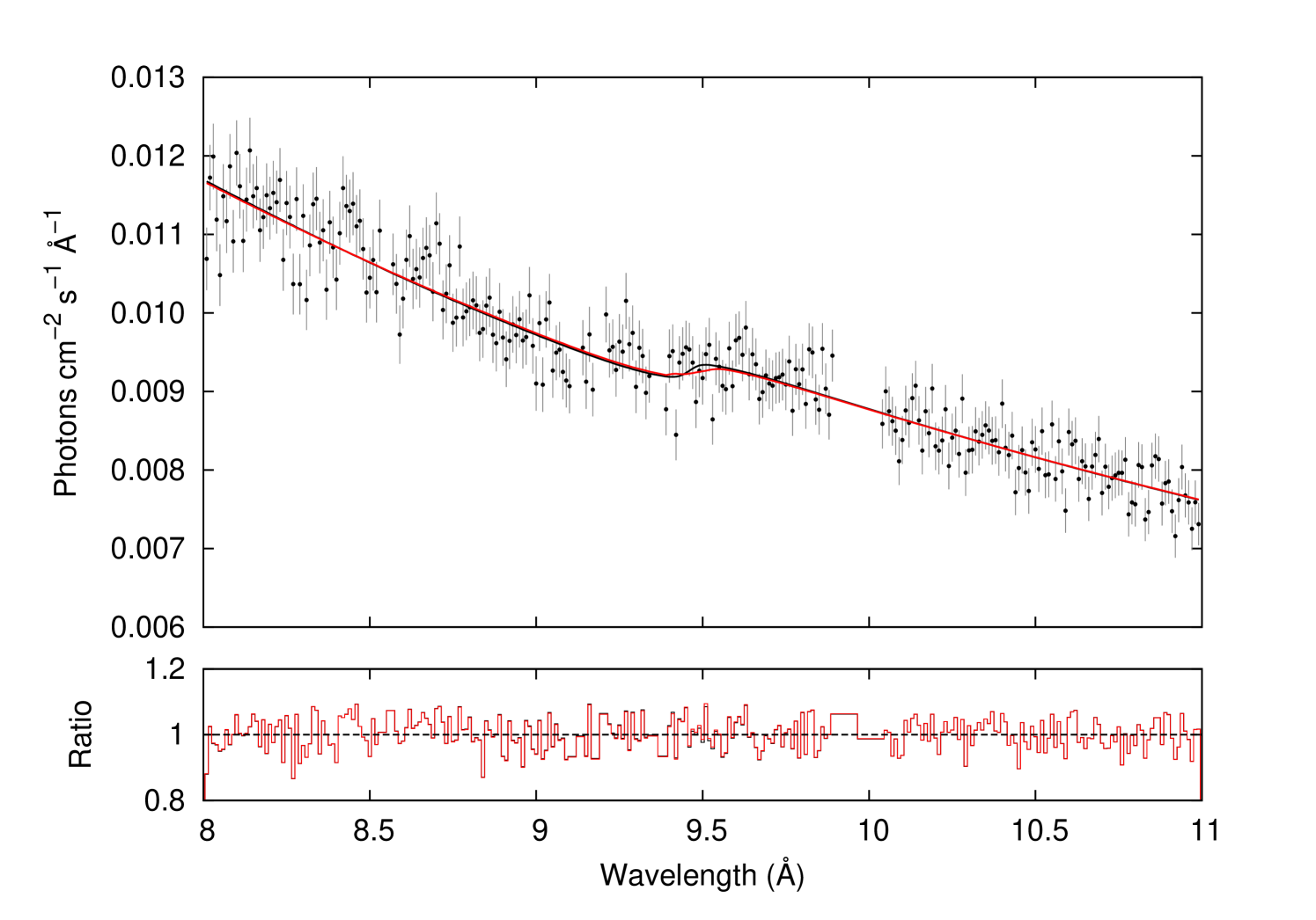
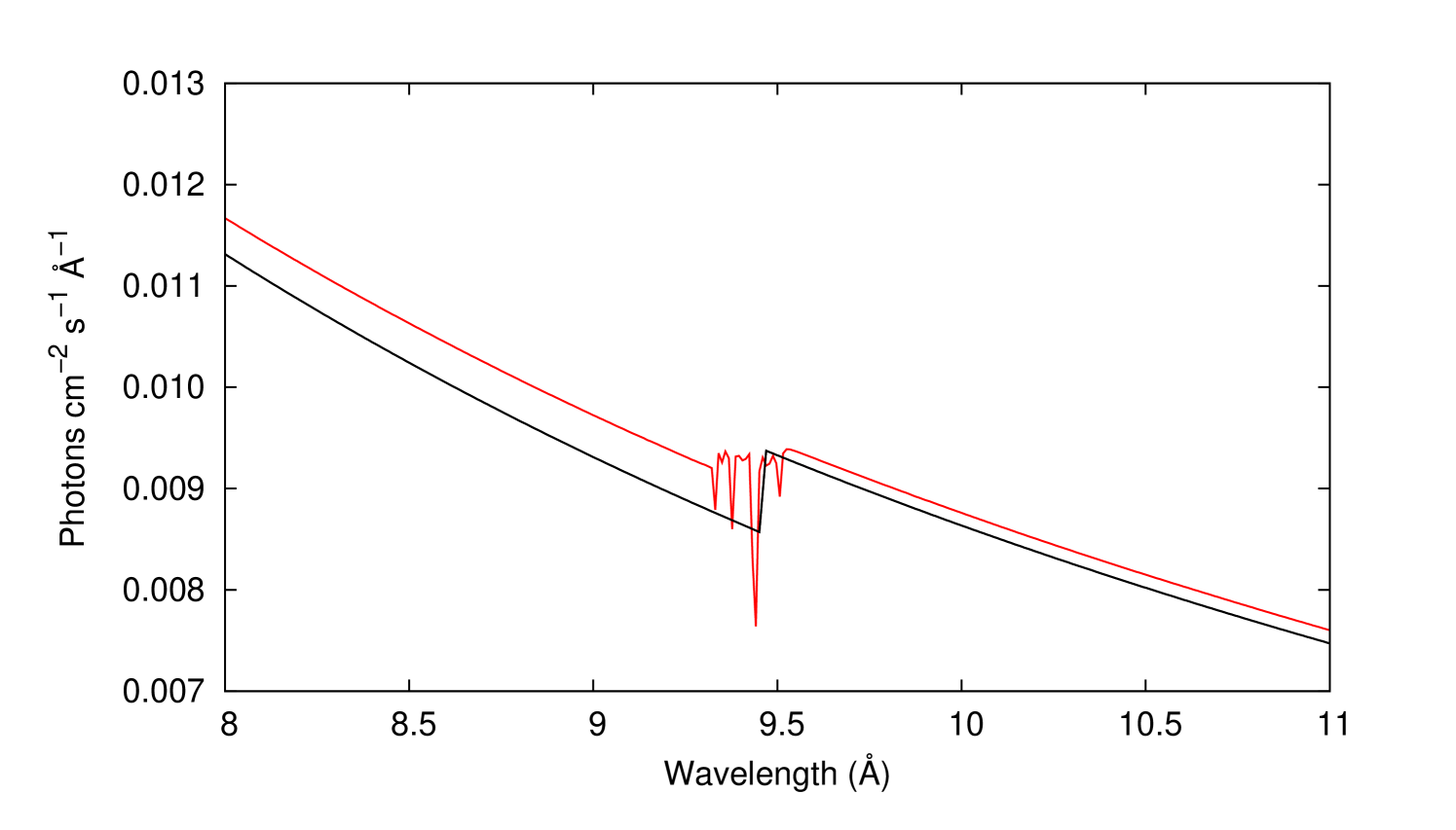
Figure 11 shows the best fit of both the TBnew (solid black line) and warmabs (solid red line) models to the XMM-Newton observations. Although the fit has been carried out simultaneously, the data are combined for visual purposes where the black dots correspond to the observations. The Mg K edge is located at $\approx 9.46$ Å. The model-to-data ratio shown in the lower panel indicates that both models fit the data satisfactorily, the best-fit parameters for both models being listed in Table 21 where abundances are given relative to Lodders (2003). It may be appreciated that the fit quality ( $\chi^{2}$ ) for both models is approximately the same although the physical predictions are different: the TBnew abundance ( $5.24^{+1.68}_{-1.52}$ ) is 16% greater than that of warmabs ( $4.51^{+2.11}_{-1.02}$ ), and the ionization parameter of the latter ( $-2.38^{+0.81}_{-0.97}$ ) indicates a strong presence of not only Mg I but also Mg II and Mg III ions. A calculation of the confidence region for the ionization parameter is included in Figure 12 where it may be noted that the best fit requires the presence of ionized states. Figure 13 shows a comparison of the models in units of flux (photons cm^-2 s^-1 Å^-1) in the Mg K-edge region: TBnew shows a simple neutral edge while the inclusion of the higher ionized species in warmabs results in a more complex and smeared edge. We have derived the Mg column densities using the ionization fractions from the warmabs fit (see Table 22), namely $(6.433\pm 1.28)\times 10^{16}$ cm^-2, $(7.085\pm 1.41)\times 10^{16}$ cm^-2, and $(1.29\pm 0.25)\times 10^{17}$ cm^-2 for Mg I–Mg III, respectively. These values are much larger than those expected in the ISM (e.g. Valencic & Smith, 2013) explaining the high abundance in both models; however, the warmabs ionization fractions agree with previous UV observations that indicate that Mg is expected to be found predominantly in ionized rather than neutral form (Gnacinski & Krogulec, 2006).

5 Summary and Conclusion

We have performed new R-matrix optical potential calculations for the K-shell photoabsorption cross sections of the Mg I–Mg X ions. Comparison with IP cross sections (Verner et al., 1993) indicates that we have computed accurate direct photoionization cross sections away from the resonant region. Concerning the Rydberg series of $1s\rightarrow np$ resonant photoabsorption below threshold, we compare to the only other existing calculations of Witthoeft et al. (2009) and Witthoeft et al. (2011) for Mg II–Mg X (i.e., excluding the all important neutral Mg I), and conclude the following. Whereas the cross sections compare well, at least for the background magnitude and the resonance strengths, between the two calculations for multiply-charged Mg ions, the two begin to differ more as the ionization stage is decreased, owing to the increased relaxation effects for low charged systems. The earlier R-matrix calculations (Witthoeft et al., 2009; Witthoeft et al., 2011) did not include relaxation effects, and as a result, their K-edge threshold positions were overestimated - by about 10 eV for Mg II, by about 5 eV for Mg III, and diminishing to roughly a constant of 2 eV for higher ionization stages. Furthermore,

Of equal importance, those earlier R-matrix calculations only treated ionized Mg ions, and no other resonant K-shell photoabsorption cross sections are available for neutral Mg I. As a result, the present calculations represent a significant improvement in the Mg ion K-shell photoabsorption database, correctly modeling all features in the vicinity of the K-edge.

These new cross sections have been included in the atomic database of the xstar modeling code (Bautista & Kallman, 2001) in order to continue the atomic data benchmarking with astronomical spectra currently being carried out by Gatuzz et al. (2013a, b) and Gorczyca et al. (2013). As an initial test, we have fitted the Mg edge in XMM-Newton spectra of the low-mass X-ray binary GS 1826-238 with models that include both the older IP cross sections of Verner et al. (1993) (TBnew) and the present cross sections (warmabs). Even though these observations are not good enough to give a reliable verdict, an interesting new finding is that most of the Mg happens to be in ionized form; this certainly justifies the present effort to compute accurate cross sections for the ionized species and perhaps explains the abundance difference (a factor of 2) with respect to the value quoted by Pinto et al. (2010).

6 Acknowledgment

This work was supported in part by a NASA APRA grant NNX11AF32G.

References

Banna et al. (1982) Banna, M. S., Slaughter, A. R., Mathews, R. D., Key, R. J., & Ballina, S. M. 1982, Chem. Phys. Lett., 92, 122
Bautista & Kallman (2001) Bautista, M. A., & Kallman, T. R. 2001, ApJS, 134, 139
Behar et al. (2001) Behar, E., Rasmussen, A. P., Griffiths, R. G., et al. 2001, A&A, 365, L242
Berrington et al. (1995) Berrington, K. A., Eissner, W., & Norrington, P. H. 1995, Comput. Phys. Commun., 92, 290
Burke (2011) Burke, P. G. 2011, R-matrix Theory of Atomic Collisions (New York: Springer)
Chen (1985) Chen, M. H. 1985, Phys. Rev. A, 31, 1449
Chen (1986) Chen, M. H. 1986, ADNDT, 34, 301
Chen & Craseman (1988) Chen, M. H. and Craseman, B. 1988, Atomic Data and Nuclear Data Tables, 38, 381
Corcoran et al. (1993) Corcoran, M. F., Swank, J. H., Serlemitsos, P. J., et al. 1993, ApJ, 412, 792
García et al. (2005) García, J., Mendoza, C., Bautista, M. A., Gorczyca, T. W., Kallman, T. R., & Palmeri, P. 2005, ApJS, 158, 68
Gatuzz et al. (2013a) Gatuzz, E., García, J., Mendoza, C., et al. 2013a, ApJ, 778, 83
Gatuzz et al. (2013b) Gatuzz, E., García, J., Mendoza, C., et al. 2013b, ApJ, 768, 60
Gorczyca (2000) Gorczyca, T. W. 2000, Phys. Rev. A, 61, 024702
Gorczyca et al. (2013) Gorczyca, T. W., Bautista, M. A., Hasoglu, M. F., et al. 2013, ApJ, 779, 78
Gorczyca et al. (2006) Gorczyca, T. W., Dumitriu, I., Hasoğlu, M. F., Korista, K. T., Badnell, N. R., Savin, D. W., & Manson, S. T. 2006, ApJ, 638, L121
Gorczyca & McLaughlin (2000) Gorczyca, T. W., & McLaughlin, B. M. 2000, J. Phys. B, 33, L859
Gorczyca & Robicheaux (1999) Gorczyca, T. W., & Robicheaux, F. 1999, Phys. Rev. A, 60, 1216
Gorczyca et al. (2003) Gorczyca, T. W., et al. 2003, ApJ, 592, 636
Gnacinski & Krogulec (2006) Gnacinski, P., & Krogulec, M. 2006, Acta Astron., 56, 373
Hasoğlu et al. (2010) Hasoğlu, M. F., Abdel-Naby, Sh. A., Gorczyca, T. W., Drake, J. J., & McLaughlin, B. M. 2010, ApJ, 724, 1296
Hasoğlu et al. (2006) Hasoğlu, M. F., Gorczyca, T. W., Korista, K. T., Manson, S. T., Badnell, N. R., & Savin, D. W. 2006, ApJ, 649, L149
Hasoğlu et al. (2008) Hasoğlu, M. F., Nikolic, D., Gorczyca, T. W., Manson, S. T., Chen, M. H., & Badnell, N. R. 2008, Phys. Rev. A, 78, 032509
Henke et al. (1993) Henke, B. L., Gullikson, E. M., & Davis, J. C. 1993, ADNDT, 54, 181
Jimenez-Garate et al. (2003) Jimenez-Garate, M. A., Schulz, N. S., & Marshall, H. L. 2003, ApJ, 590, 432
Juett et al. (2004) Juett, A. M., Schulz, N. S., & Chakrabarty, D. 2004, ApJ, 612, 308
Juett et al. (2006) Juett, A. M., Schulz, N. S., Chakrabarty, D., & Gorczyca, T. W. 2006, ApJ, 648, 1066
Kalberla et al. (2005) Kalberla, P. M. W., Burton, W. B., Hartmann, D., Arnal, E. M., Bajaja, E., Morras, R., & Pöppel, W. G. L. 2005, A&A, 440, 775
Kaspi & Behar (2006) Kaspi, S., & Behar, E. 2006, ApJ, 636, 674
Lobban et al. (2011) Lobban, A. P., Reeves, J. N., Miller, L., et al. 2011, MNRAS, 414, 1965
Lodders (2003) Lodders, K. 2003, ApJ, 591, 1220
Matsushita et al. (2007) Matsushita, K., Fukazawa, Y., Hughes, J. P., et al. 2007, PASJ, 59, 327
Nousek & Shue (1989) Nousek, J. A., & Shue, D. R. 1989, ApJ, 342, 1207
Paerels & Kahn (2003) Paerels, F. B. S., & Kahn, S. M. 2003, ARA&A, 41, 291
Palmeri et al. (2008) Palmeri, P., Quinet, P., Mendoza, C., Bautista, M. A., Garcia, J., & Kallman, T. R. 2008, ApJS, 177, 408
Pinto et al. (2010) Pinto, C., Kaastra, J. S., Costantini, E., & Verbunt, F. 2010, A&A, 521, A79
Pounds & Page (2005) Pounds, K. A., & Page, K. L. 2005, MNRAS, 360, 1123
Sakelliou et al. (2002) Sakelliou, I., Peterson, J. R., Tamura, T., et al. 2002, A&A, 391, 903
Schulz et al. (2010) Schulz, N. S., Nowak, M. A., Chakrabarty, D., & Canizares, C. R. 2010, ApJ, 725, 2417
Sezer et al. (2011) Sezer, A., Gök, F., Hudaverdi, M., Kimura, M., & Ercan, E. N. 2011, MNRAS, 415, 301
Smith (1960) Smith, F. T. 1960, Phys. Rev., 118, 349
Tsuru et al. (2007) Tsuru, T. G., Ozawa, M., Hyodo, Y., et al. 2007, PASJ, 59, 269
Valencic & Smith (2013) Valencic, L. A., & Smith, R. K. 2013, ApJ, 770, 22
Verner et al. (1996) Verner, D. A., Ferland, G. J. Korista, K. T., & Yakovlev, D. G. 1996, ApJ, 465, 487
Verner et al. (1993) Verner, D. A., Yakovlev, D. G., Band, I. M., & Trzhaskovskaya, M. B. 1993, ADNDT, 55, 233
Witthoeft et al. (2009) Witthoeft, M. C., Bautista, M. A., Mendoza, C., Kallman, T. R., Palmeri, P., & Quinet, P. 2009, ApJS, 182, 127
Witthoeft et al. (2011) Witthoeft, M. C., García, J., Kallman, T. R., et al. 2011, ApJS, 192, 7
Wojdowski et al. (2003) Wojdowski, P. S., Liedahl, D. A., Sako, M., Kahn, S. M., & Paerels, F. 2003, ApJ, 582, 959
Yamaguchi et al. (2012) Yamaguchi, H., Tanaka, M., Maeda, K., et al. 2012, ApJ, 749, 137

Refer to caption — Figure 1: Mg I photoabsorption cross sections. Pre-convoluted cross section obtained by damping the core excited states (see Table 1) with an artificially smaller 0.001 Ryd spectator Auger width, then performing a Lorentzian convolution with the calculated Auger-width of $0.0254$ Ryd for the $1s^{2}2s^{2}2p^{6}3s^{2}\,{}^{2}S$ state (see Table 11) to get the final cross section. Also shown are the IP results (Verner et al., 1993) and solid-state experimental results (Henke et al., 1993).

Table 1: Energies (Ryd) of the Mg II target states and Mg I ground state. Also shown are NIST spectroscopic values and HFR1 results (Palmeri et al., 2008).

State	Present	NIST	HFR1
$1s^{2}2s^{2}2p^{6}3s^{2}\ {}^{1}S$	$-0.5428$	$-0.5620$
$1s^{2}2s^{2}2p^{6}3s\ ^{2}S$	$0.0000$	$0.0000$	$0.0000$
$1s^{2}2s^{2}2p^{6}3p\ ^{2}P$	$0.3162$	$0.3256$	$0.3300$
$1s^{2}2s^{2}2p^{5}3s^{2}\ {}^{2}P$	$3.8240$	$3.6745$	$3.6235$
$1s^{2}2s2p^{6}3s^{2}\ {}^{2}S$	$6.7244$
$1s^{2}s22p^{6}3s^{2}\ {}^{2}S$	$95.8157$		$95.8295$
$1s^{2}s22p^{6}3s(^{1}S)3p\ ^{2}P$	$96.1441$		$96.1612$
$1s2s^{2}2p^{6}3s(^{3}S)3p\ ^{2}P$	$96.3185$		$96.5066$

Table 2: Energies (Ryd) of the Mg III target states and Mg II ground state.

State	Present	NIST
$1s^{2}2s^{2}2p^{6}3s\ ^{2}S)$	$-1.0928$	$-1.1051$
$1s^{2}2s^{2}2p^{6}\ {}^{1}S$	$0.0000$	$0.0000$
$1s^{2}2s^{2}2p^{5}3s\ ^{3}P$	$3.8897$	$3.8847$
$1s^{2}2s^{2}2p^{5}3s\ ^{1}P$	$3.9384$	$3.9324$
$1s^{2}2s^{2}2p^{5}3p\ ^{3}S$	$4.2561$	$4.2591$
$1s^{2}2s^{2}2p^{5}3p\ ^{1}P$	$4.3615$	$4.3593$
$1s^{2}2s^{2}2p^{5}3p\ ^{3}P$	$4.3624$	$4.3658$
$1s^{2}2s^{2}2p^{5}3p\ ^{1}S$	$4.5778$	$4.5200$
$1s^{2}2s^{2}2p^{5}3d\ ^{3}P$	$4.8345$	$4.8360$
$1s^{2}2s^{2}2p^{5}3d\ ^{1}P$	$4.8821$	$4.8858$
$1s^{2}2s2p^{6}3s\ ^{3}S$	$6.7391$
$1s^{2}2s2p^{6}3s\ ^{1}S$	$6.8192$
$1s^{2}2s2p^{6}3p\ ^{3}P$	$7.1714$
$1s^{2}2s2p^{6}3p\ ^{1}P$	$7.2026$	$7.204$
$1s2s^{2}2p^{6}3s\ ^{3}S$	$95.9528$
$1s2s^{2}2p^{6}3s\ ^{1}S$	$96.0030$
$1s2s^{2}2p^{6}3p\ ^{3}P$	$96.3928$
$1s2s^{2}2p^{6}3p\ ^{1}P$	$96.4199$

Table 3: Energies (Ryd) of the Mg IV target states and Mg III ground state.

State	Present	NIST
$1s^{2}2s^{2}2p^{6}\ {}^{1}S$	$-6.0727$	$-5.8955$
$1s^{2}2s^{2}2p^{5}\ {}^{2}P$	$0.0000$	$0.0000$
$1s^{2}2s2p^{6}\ {}^{2}S$	$2.6694$	$2.8321$
$1s2s^{2}2p^{6}\ {}^{2}S$	$91.9430$

Table 4: Energies (Ryd) of the Mg V target states and Mg IV ground state.

State	Present	NIST
$1s^{2}2s^{2}p^{5}\ {}^{2}P$	$-8.2847$	$-8.0471$
$1s^{2}2s^{2}p^{4}\ {}^{3}P$	$0.0000$	$0.0000$
$1s^{2}2s^{2}p^{4}\ {}^{1}D$	$0.3369$	$0.3194$
$1s^{2}2s^{2}p^{4}\ {}^{1}S$	$0.7227$	$0.6963$
$1s^{2}2s^{2}p^{5}\ {}^{3}P$	$2.3940$	$2.5803$
$1s^{2}2s^{2}p^{5}\ {}^{1}P$	$3.4698$	$3.6142$
$1s^{2}2p^{6}\ {}^{1}S$	$5.9444$	$6.0335$
$1s2s^{2}2p^{5}\ {}^{3}P$	$92.9165$
$1s2s^{2}2p^{5}\ {}^{1}P$	$93.3603$
$1s2s2p^{6}\ {}^{3}S$	$95.3646$
$1s2s2p^{6}\ {}^{1}S$	$96.0868$

Table 5: Energies (Ryd) of the Mg VI target states and Mg V ground state.

State	Present	NIST
$1s^{2}2s^{2}p^{4}\ {}^{3}P$	$-10.3562$	$-10.3880$
$1s^{2}2s^{2}2p^{3}\ {}^{4}S$	$0.00000$	$0.0000$
$1s^{2}2s^{2}2p^{3}\ {}^{2}D$	$0.52952$	$0.5045$
$1s^{2}2s^{2}2p^{3}\ {}^{2}P$	$0.79048$	$0.7654$
$1s^{2}2s2p^{4}\ {}^{4}P$	$2.24151$	$2.2682$
$1s^{2}2s2p^{4}\ {}^{2}D$	$3.12096$	$3.1144$
$1s^{2}2s2p^{4}\ {}^{2}S$	$3.67859$	$3.6617$
$1s^{2}2s2p^{4}\ {}^{2}P$	$3.90098$	$3.8805$
$1s^{2}2p^{5}\ {}^{2}P$	$5.92479$	$5.9482$
$1s2s^{2}2p^{4}\ {}^{4}P$	$93.60545$
$1s2s^{2}2p^{4}\ {}^{2}D$	$94.23068$
$1s2s^{2}2p^{4}\ {}^{2}P$	$94.36199$
$1s2s^{2}2p^{4}\ {}^{2}S$	$94.61941$
$1s2s2p^{5}(^{3}P)\ ^{4}P$	$95.82506$
$1s2s2p^{5}(^{3}P)\ ^{2}P$	$96.70406$
$1s2s2p^{5}(^{1}P)\ ^{2}P$	$97.27956$
$1s2p^{6}\ {}^{2}S$	$99.41050$

Table 6: Energies (Ryd) of the Mg VII target states and Mg VI ground state.

State	Present	NIST
$1s^{2}2s^{2}2p^{3}\ {}^{4}S$	$-13.7208$	$-13.7260$
$1s^{2}2s^{2}2p^{2}\ {}^{3}P$	$0.0000$	$0.0000$
$1s^{2}2s2p^{3}\ {}^{5}S$	$1.0016$	$1.0580$
$1s^{2}2s2p^{3}\ {}^{3}D$	$2.0873$	$2.1044$
$1s^{2}2s2p^{3}\ {}^{3}P$	$2.4774$	$2.4870$
$1s^{2}2s2p^{3}\ {}^{3}S$	$3.2739$	$3.2817$
$1s^{2}2p^{4}\ {}^{3}P$	$4.8865$	$4.9331$
$1s2s^{2}2p^{3}\ {}^{5}S$	$93.6369$
$1s2s^{2}2p^{3}\ {}^{3}D$	$94.4994$
$1s2s^{2}2p^{3}\ {}^{3}S$	$94.7250$
$1s2s^{2}2p^{3}\ {}^{3}P$	$94.7628$
$1s2s2p^{4}\ {}^{5}P$	$95.4771$
$1s2s2p^{4}(^{4}P)\ ^{3}P$	$96.6606$
$1s2s2p^{4}\ {}^{3}D$	$96.6883$
$1s2s2p^{4}\ {}^{3}S$	$97.3056$
$1s2s2p^{4}(^{2}P)\ ^{3}P$	$97.5790$
$1s2p^{5}\ {}^{3}P$	$99.2593$

Table 7: Energies (Ryd) of the Mg VIII target states and Mg VII ground state.

State	Present	NIST
$1s^{2}2s^{2}2p^{2}\ {}^{3}P$	$-16.6018$	$-16.5380$
$1s^{2}2s^{2}2p\ ^{2}P$	$0.0000$	$0.0000$
$1s^{2}2s2p^{2}\ {}^{4}P$	$1.0960$	$1.1799$
$1s^{2}2s2p^{2}\ {}^{2}D$	$2.0518$	$2.0967$
$1s^{2}2s2p^{2}\ {}^{2}S$	$2.7119$	$2.6981$
$1s^{2}2s2p^{2}\ {}^{2}P$	$2.8492$	$2.8965$
$1s^{2}2p^{3}\ {}^{4}S$	$3.6653$	$3.7490$
$1s^{2}2p^{3}\ {}^{2}D$	$4.1728$	$4.2244$
$1s^{2}2p^{3}\ {}^{2}P$	$4.7639$	$4.7621$
$1s2s^{2}2p^{2}\ {}^{4}P$	$94.9623$
$1s2s^{2}2p^{2}\ {}^{2}D$	$95.6660$
$1s2s^{2}2p^{2}\ {}^{2}P$	$95.8214$
$1s2s^{2}2p^{2}\ {}^{2}S$	$96.0915$
$1s2s2p^{3}\ {}^{4}D$	$96.5601$
$1s2s2p^{3}\ {}^{4}S$	$96.6315$
$1s2s2p^{3}\ {}^{4}P$	$97.0167$
$1s2s2p^{3}\ {}^{2}D$	$97.5622$
$1s2s2p^{3}\ {}^{4}S$	$97.8941$
$1s2s2p^{3}\ {}^{2}P$	$98.0187$
$1s2s2p^{3}\ {}^{2}D$	$98.1266$
$1s2s2p^{3}\ {}^{2}P$	$98.5930$
$1s2s2p^{3}\ {}^{2}S$	$98.6195$
$1s2p^{4}\ {}^{4}P$	$99.0702$
$1s2p^{4}\ {}^{2}D$	$99.7024$
$1s2p^{4}\ {}^{2}P$	$99.8864$
$1s2p^{4}\ {}^{2}S$	$100.6505$

Table 8: Energies (Ryd) of the Mg IX target states and Mg VIII ground state.

State	Present	NIST
$1s^{2}2s^{2}2p\ ^{2}P$	$-19.5175$	$-19.5450$
$1s^{2}2s^{2}\ {}^{1}S$	$0.0000$	$0.0000$
$1s^{2}2s2p\ ^{3}P$	$1.2720$	$1.3020$
$1s^{2}2s2p\ ^{1}P$	$2.4716$	$2.4758$
$1s^{2}2p^{2}\ {}^{3}P$	$3.3112$	$3.3555$
$1s^{2}2p^{2}\ {}^{1}D$	$3.6698$	$3.6915$
$1s^{2}2p^{2}\ {}^{1}S$	$4.6220$	$4.5530$
$1s2s^{2}2p\ ^{3}P$	$96.3470$
$1s2s^{2}2p\ ^{1}P$	$96.9743$	$97.1192$
$1s2s(^{3}S)2p^{2}\ {}^{3}D$	$97.9274$
$1s2s(^{1}S)2p^{2}\ {}^{3}P$	$97.9575$
$1s2s(^{3}S)2p^{2}\ {}^{3}S$	$98.6507$
$1s2s(^{3}S)2p^{2}\ {}^{1}D$	$98.7677$
$1s2s(^{3}S)2p^{2}\ {}^{3}P$	$98.8326$
$1s2s(^{3}S)2p^{2}\ {}^{1}P$	$99.3433$
$1s2s(^{1}S)2p^{2}\ {}^{1}S$	$99.4907$
$1s2p^{3}\ {}^{3}D$	$99.6064$
$1s2p^{3}\ {}^{3}S$	$99.9059$
$1s2p^{3}\ {}^{1}D$	$100.1887$
$1s2p^{3}\ {}^{3}P$	$100.2962$
$1s2p^{3}\ {}^{1}P$	$100.8812$

Table 9: Energies (Ryd) of the Mg X target states and Mg IX ground state.

State	Present	NIST
$1s^{2}2s^{2}\ {}^{1}$	$-24.0872$	$-24.1060$
$1s^{2}2s\ ^{2}S$	$0.0000$	$0.0000$
$1s^{2}2p\ ^{2}P$	$1.4855$	$1.4823$
$1s2s^{2}\ {}^{2}S$	$96.4886$
$1s2s(^{1}S)2p\ ^{2}P$	$97.9741$	$98.1544$
$1s2s(^{3}S)2p\ ^{2}P$	$98.5011$	$98.6810$
$1s2p^{2}\ {}^{2}D$	$99.0911$	$99.2730$
$1s2p^{2}\ {}^{2}P$	$99.3072$	$99.5100$
$1s2p^{2}\ {}^{2}S$	$100.2157$	$100.310$

Table 10: Energies (Ryd) of the Mg XI target states and Mg X ground state.

State	Present	NIST
$1s^{2}2s\ ^{2}S$	$-26.9543$	$-27.0100$
$1s^{2}\ {}^{1}S$	$0.0000$	$0.0000$
$1s2s\ ^{3}S$	$97.6959$	$97.8349$
$1s2p\ ^{3}P$	$98.5492$	$98.7331$
$1s2s\ ^{1}S$	$98.6309$	$98.7702$
$1s2p\ ^{1}P$	$99.2148$	$99.3884$

Table 11: Present Auger widths (in Ryd) for the three Mg II autoionizing target states above the K-shell threshold (see Table 1). Also shown are the level-averaged HFR1 results (Palmeri et al., 2008).

	State	Present	HFR1
1	$1s^{2}2s22p^{6}3s^{2}\ {}^{2}S$	2.54 $\times 10^{-2}$	2.39 $\times 10^{-2}$
2	$1s^{2}2s22p^{6}3s(^{1}S)3p\ ^{2}P$	1.73 $\times 10^{-2}$	2.37 $\times 10^{-2}$
3	$1s2s^{2}2p^{6}3s(^{3}S)3p\ ^{2}P$	2.26 $\times 10^{-2}$	2.36 $\times 10^{-2}$

Table 12: Present Auger widths (in Ryd) for the four Mg III autoionizing target states above the K-shell threshold (see Table 2). Also shown are the level-averaged HFR1 results (Palmeri et al., 2008).

	State	Present	MCBP
1	$1s2s^{2}2p^{6}3s\ ^{3}S$	2.39 $\times 10^{-2}$	2.68 $\times 10^{-2}$
2	$1s2s^{2}2p^{6}3s\ ^{1}S$	2.41 $\times 10^{-2}$	2.52 $\times 10^{-2}$
3	$1s2s^{2}2p^{6}3p\ ^{3}P$	2.37 $\times 10^{-2}$	2.45 $\times 10^{-2}$
4	$1s2s^{2}2p^{6}3p\ ^{1}P$	2.33 $\times 10^{-2}$	2.44 $\times 10^{-2}$

Table 13: Present Auger widths (in Ryd) for the Mg IV autoionizing target state above the K-shell threshold (see Table 3). Also shown are level-averaged HFR1 widths (Palmeri et al., 2008) and AUTOSTRUCTURE results (Gorczyca et al., 2003).

State		Present		HFR1		AUTO
$1s2s^{2}2p^{6}\ {}^{2}S$		2.45 $\times 10^{-2}$		2.45 $\times 10^{-3}$		3.01 $\times 10^{-2}$

Table 14: Present Auger widths (in Ryd) for the four Mg V autoionizing target states above the K-shell threshold (see Table 4). Also shown are the level-averaged results (Palmeri et al., 2008).

	State	Present	MCBP
1	$1s2s^{2}2p^{5}\ {}^{3}P$	2.13 $\times 10^{-2}$	2.22 $\times 10^{-2}$
2	$1s2s^{2}2p^{5}\ {}^{1}P$	2.02 $\times 10^{-2}$	2.06 $\times 10^{-2}$
3	$1s2s2p^{6}\ {}^{3}S$	1.90 $\times 10^{-2}$	2.00 $\times 10^{-2}$
4	$1s2s2p^{6}\ {}^{1}S$	2.84 $\times 10^{-2}$	3.05 $\times 10^{-2}$

Table 15: Present Auger widths (in Ryd) for the eight Mg VI autoionizing target states above the K-shell threshold (see Table 5). Also shown are the level-averaged HFR1 results (Palmeri et al., 2008).

	State	Present	HFR1
1	$1s2s^{2}2p^{4}\ {}^{4}P$	1.66 $\times 10^{-2}$	1.64 $\times 10^{-2}$
2	$1s2s^{2}2p^{4}\ {}^{2}D$	2.00 $\times 10^{-2}$	1.96 $\times 10^{-2}$
3	$1s2s^{2}2p^{4}\ {}^{2}P$	1.45 $\times 10^{-2}$	1.39 $\times 10^{-2}$
4	$1s2s^{2}2p^{4}\ {}^{2}S$	1.87 $\times 10^{-2}$	1.83 $\times 10^{-2}$
5	$1s2s2p^{5}(^{3}P)\ ^{4}P$	1.49 $\times 10^{-2}$	1.46 $\times 10^{-2}$
6	$1s2s2p^{5}(^{3}P)\ ^{2}P$	1.97 $\times 10^{-2}$	1.89 $\times 10^{-2}$
7	$1s2s2p^{5}(^{1}P)\ ^{2}P$	2.02 $\times 10^{-2}$	2.03 $\times 10^{-2}$
8	$1s2p^{6}\ {}^{2}S$	1.89 $\times 10^{-2}$	1.87 $\times 10^{-2}$

Table 16: Present Auger widths (in Ryd) for the ten Mg VII autoionizing target states above the K-shell threshold (see Table 6). Also shown are level-averaged HFR1 (Palmeri et al., 2008), level-averaged MCBP (Hasoğlu et al., 2008), and level-averaged MCDF (Hasoğlu et al., 2008) widths.

	State	Present	HFR1	MCDF	MCBP
1	$1s2s^{2}2p^{3}\ {}^{5}S$	9.31 $\times 10^{-3}$	9.53 $\times 10^{-3}$	1.36 $\times 10^{-2}$	9.95 $\times 10^{-3}$
2	$1s2s^{2}2p^{3}\ {}^{3}D$	1.54 $\times 10^{-2}$	1.53 $\times 10^{-2}$	1.91 $\times 10^{-2}$	1.59 $\times 10^{-2}$
3	$1s2s^{2}2p^{3}\ {}^{3}S$	5.82 $\times 10^{-3}$	5.52 $\times 10^{-3}$	8.89 $\times 10^{-3}$	5.72 $\times 10^{-3}$
4	$1s2s^{2}2p^{3}\ {}^{3}P$	1.45 $\times 10^{-2}$	1.40 $\times 10^{-2}$	1.77 $\times 10^{-2}$	1.46 $\times 10^{-2}$
5	$1s2s2p^{4}\ {}^{5}P$	8.57 $\times 10^{-3}$	8.56 $\times 10^{-3}$
6	$1s2s2p^{4}(^{4}P)\ ^{3}P$	1.18 $\times 10^{-2}$	1.15 $\times 10^{-2}$
7	$1s2s2p^{4}\ {}^{3}D$	1.37 $\times 10^{-2}$	1.36 $\times 10^{-2}$
8	$1s2s2p^{4}\ {}^{3}S$	1.10 $\times 10^{-2}$	1.08 $\times 10^{-2}$
9	$1s2s2p^{4}(^{2}P)\ ^{3}P$	1.50 $\times 10^{-2}$	1.51 $\times 10^{-2}$
10	$1s2p^{5}\ {}^{3}P$	1.46 $\times 10^{-2}$	1.48 $\times 10^{-2}$

Table 17: Present Auger widths (in Ryd) for the 17 Mg VIII autoionizing target states above the K-shell threshold (see Table 7). Also shown are level-averaged HFR1 (Palmeri et al., 2008), level-averaged MCDF (Chen & Craseman, 1988), and level-averaged MCBP (Hasoğlu et al., 2006) widths.

	State	Present	HFR1	MCDF	MCBP
1	$1s2s^{2}2p^{2}\ {}^{4}P$	8.73 $\times 10^{-3}$	7.81 $\times 10^{-3}$	8.98 $\times 10^{-3}$	9.06 $\times 10^{-3}$
2	$1s2s^{2}2p^{2}\ {}^{2}D$	1.30 $\times 10^{-2}$	1.23 $\times 10^{-2}$	1.27 $\times 10^{-2}$	1.30 $\times 10^{-2}$
3	$1s2s^{2}2p^{2}\ {}^{2}P$	5.63 $\times 10^{-3}$	4.60 $\times 10^{-3}$	5.37 $\times 10^{-3}$	5.32 $\times 10^{-3}$
4	$1s2s^{2}2p^{2}\ {}^{2}S$	1.15 $\times 10^{-2}$	1.00 $\times 10^{-2}$	1.12 $\times 10^{-2}$	1.11 $\times 10^{-2}$
5	$1s2s(^{3}S)2p^{3}\ {}^{4}D$	8.35 $\times 10^{-3}$	8.71 $\times 10^{-3}$	8.17 $\times 10^{-3}$
6	$1s2s(^{1}S)2p^{3}\ {}^{4}S$	1.46 $\times 10^{-3}$	6.92 $\times 10^{-4}$	1.91 $\times 10^{-3}$
7	$1s2s(^{3}S)2p^{3}\ {}^{4}P$	6.40 $\times 10^{-3}$	6.63 $\times 10^{-3}$	6.28 $\times 10^{-3}$
8	$1s2s(^{1}S)2p^{3}\ {}^{2}D$	1.13 $\times 10^{-2}$	1.06 $\times 10^{-2}$	1.15 $\times 10^{-2}$
9	$1s2s(^{3}S)2p^{3}\ {}^{4}S$	7.63 $\times 10^{-3}$	6.97 $\times 10^{-3}$	8.51 $\times 10^{-3}$
10	$1s2s(^{1}S)2p^{3}\ {}^{2}P$	9.45 $\times 10^{-3}$	8.45 $\times 10^{-3}$	9.59 $\times 10^{-3}$
11	$1s2s(^{3}S)2p^{3}\ {}^{2}D$	1.33 $\times 10^{-2}$	1.30 $\times 10^{-2}$	1.39 $\times 10^{-2}$
12	$1s2s(^{3}S)2p^{3}\ {}^{2}P$	1.14 $\times 10^{-2}$	1.07 $\times 10^{-2}$	1.16 $\times 10^{-2}$
13	$1s2s(^{3}S)2p^{3}\ {}^{2}S$	2.86 $\times 10^{-3}$	3.71 $\times 10^{-3}$	3.41 $\times 10^{-3}$
14	$1s2p^{4}\ {}^{4}P$	8.38 $\times 10^{-3}$	6.48 $\times 10^{-3}$	8.73 $\times 10^{-3}$
15	$1s2p^{4}\ {}^{2}D$	1.33 $\times 10^{-2}$	1.01 $\times 10^{-2}$	1.37 $\times 10^{-2}$
16	$1s2p^{4}\ {}^{2}P$	8.34 $\times 10^{-3}$	6.47 $\times 10^{-3}$	8.58 $\times 10^{-3}$
17	$1s2p^{4}\ {}^{2}S$	9.18 $\times 10^{-3}$	6.72 $\times 10^{-3}$	9.48 $\times 10^{-3}$

Table 18: Present Auger widths (in Ryd) for the Mg IX autoionizing target states above the K-shell threshold (see Table 8). Also shown are level-averaged HFR1 (Palmeri et al., 2008), level-averaged MCDF (Chen, 1985), and level-averaged MBCP (Gorczyca et al., 2003) widths.

	State	Present	HFR1	MCDF	MCBP
1	$1s2s^{2}2p\ ^{3}P$	7.44 $\times 10^{-3}$	7.35 $\times 10^{-3}$	7.61 $\times 10^{-3}$	7.89 $\times 10^{-3}$
2	$1s2s^{2}2p\ ^{1}P$	5.26 $\times 10^{-3}$	4.84 $\times 10^{-3}$	5.08 $\times 10^{-3}$	5.12 $\times 10^{-3}$
3	$1s2s(^{3}S)2p^{2}\ {}^{3}D$	6.62 $\times 10^{-3}$	5.95 $\times 10^{-3}$	5.87 $\times 10^{-3}$
4	$1s2s(^{1}S)2p^{2}\ {}^{3}P$	8.51 $\times 10^{-4}$	2.30 $\times 10^{-3}$	2.01 $\times 10^{-3}$
5	$1s2s(^{3}S)2p^{2}\ {}^{3}S$	3.36 $\times 10^{-3}$	3.29 $\times 10^{-3}$	3.10 $\times 10^{-3}$
6	$1s2s(^{3}S)2p^{2}\ {}^{1}D$	1.12 $\times 10^{-2}$	1.17 $\times 10^{-2}$	1.23 $\times 10^{-2}$
7	$1s2s(^{3}S)2p^{2}\ {}^{3}P$	6.06 $\times 10^{-3}$	6.27 $\times 10^{-3}$	6.40 $\times 10^{-3}$
8	$1s2s(^{3}S)2p^{2}\ {}^{1}P$	2.44 $\times 10^{-3}$	2.16 $\times 10^{-3}$	1.89 $\times 10^{-3}$
9	$1s2s(^{1}S)2p^{2}\ {}^{1}S$	8.24 $\times 10^{-3}$	8.03 $\times 10^{-3}$	8.76 $\times 10^{-3}$
10	$1s2p^{3}\ {}^{3}D$	8.43 $\times 10^{-3}$	8.80 $\times 10^{-3}$	8.50 $\times 10^{-3}$
11	$1s2p^{3}\ {}^{3}S$		1.14 $\times 10^{-5}$	1.49 $\times 10^{-5}$
12	$1s2p^{3}\ {}^{1}D$	8.39 $\times 10^{-3}$	8.61 $\times 10^{-3}$	8.27 $\times 10^{-3}$
13	$1s2p^{3}\ {}^{3}P$	5.32 $\times 10^{-3}$	5.53 $\times 10^{-3}$	5.31 $\times 10^{-3}$
14	$1s2p^{3}\ {}^{1}P$	5.05 $\times 10^{-3}$	5.27 $\times 10^{-3}$	5.03 $\times 10^{-3}$

Table 19: Present Auger widths (in Ryd) for the Mg X autoionizing target states above the K-shell threshold (see Table 9). Also shown are level-averaged HFR1 (Palmeri et al., 2008), level-averaged MCDF(Chen, 1986), and level-averaged MBCP (Gorczyca et al., 2006) widths.

	State	Present	HFR1	MCDF	MCBP
1	$1s2s^{2}\ {}^{2}S$	6.27 $\times 10^{-3}$	5.81 $\times 10^{-3}$	5.42 $\times 10^{-3}$	6.28 $\times 10^{-3}$
2	$1s2s(^{1}S)2p\ ^{2}P$	4.06 $\times 10^{-3}$	4.02 $\times 10^{-3}$	3.53 $\times 10^{-3}$
3	$1s2s(^{3}S)2p\ ^{2}P$	2.89 $\times 10^{-4}$	3.21 $\times 10^{-4}$	5.44 $\times 10^{-4}$
4	$1s2p^{2}\ {}^{2}D$	6.39 $\times 10^{-3}$	6.90 $\times 10^{-3}$	6.61 $\times 10^{-3}$
5	$1s2p^{2}\ {}^{2}P$		3.98 $\times 10^{-5}$	3.37 $\times 10^{-5}$
6	$1s2p^{2}\ {}^{2}S$	9.41 $\times 10^{-4}$	1.05 $\times 10^{-3}$	1.10 $\times 10^{-3}$

Table 20: XMM-Newton RGS observations used in this paper

ObsID	Date	Exposure (ks)
0150390101	2003 April 6	106
0150390301	2003 April 8	91.5

Table 21: GS1826-238 Mg Edge Fit

Parameter	TBnew	warmabs
$N_{\rm H}(10^{21}$ cm ${}^{-2})^{a}$	$1.68$	$1.68$
A ${}_{\rm Mg}^{b}$	$5.24^{+1.68}_{-1.52}$	$4.51^{+2.11}_{-1.02}$
$\log\xi$		$-2.38^{+0.81}_{-0.97}$
$\chi^{2}$	$0.974$	$0.974$

^a^afootnotetext: Fixed to the

21

cm value (Kalberla et al., 2005).

^b^bfootnotetext: Abundances relative to the solar values of Lodders (2003).

Table 22: Mg Ionic Column Densities

Ion	Ionization Fraction	Column Density
Mg I	$0.24\pm 0.04$	$6.43\pm 1.28$
Mg II	$0.26\pm 0.05$	$7.08\pm 1.41$
Mg III	$0.48\pm 0.09$	$12.98\pm 2.51$

Note. — Mg column densities in units of $10^{16}$ cm^-2. Values are derived from the warmabs fit using the Mg solar abundance in Lodders (2003).