subsecref \newrefsubsecname = \RSsectxt \RS@ifundefinedthmref \newrefthmname = theorem \RS@ifundefinedlemref \newreflemname = lemma
Katu: a fast open-source full lepto-hadronic kinetic code suitable for Bayesian inference modeling of blazars
Abstract
In the modelling of blazars and other radiating plasma flows, correctly evolving in time a series of kinetic equation coupled for different particle species is a computationally challenging problem. In this paper we introduce the code Katu, capable of simultaneously evolving a large number of particle species including photons, leptons and hadrons and their interactions. For each particle, the numerical expressions for the kinetic equations are optimized for efficiency and the code is written to easily allow for extensions and modifications. Additionally, we tie Katu to two pieces of statistical software, emcee and pymultinest, which makes a suite ready to apply to blazars and extract relevant statistical information from their electromagnetic (and neutrino, if applicable) flux. As an example, we apply Katu to Mrk 421 and compare a leptonic and a leptohadronic model. In this first ever direct Bayesian comparison between full kinetic simulations of these models, we find substantial evidence (Bayes factor ) for the leptohadronic model purely from the electromagnetic spectrum. The code is available online at https://github.com/hveerten/katu under the LGPL license111Alternatively, a mirror is maintained at https://gitlab.com/Noxbru/Katu.
keywords:
Radiation mechanisms: non-thermal, methods: statistical, methods: numerical, BL Lacertae objects: individual: Mrk 421.1 Introduction
Simulating the behaviour of energetic particles both individually and collectively is relevant in many fields of particle physics and astrophysics. In the first case, understanding how a particle emits and interacts with others has allowed us to build the theory of the standard model of particle physics. In the second case, by putting together all the results from the first, we can develop theories to explain the emission from astrophysical objects such as stars, planetary nebulae or, as for this work, blazars.
The theory of emission processess that occur between interacting non-thermal distributions of lepto-hadronic particles has evolved over many years (see e.g. Jones, 1968; Lightman & Zdziarski, 1987; Mastichiadis & Kirk, 1992), as have methods to solve these systems numerically (e.g. Mastichiadis & Kirk, 1995). More recently, the increase in computational power has allowed for the development of more complete models with better approximations to the different processes and models that deal explicitly with more kinds of particles, such as Mastichiadis et al. (2005); Dimitrakoudis et al. (2012); Cerruti et al. (2015); Petropoulou et al. (2015) and Gao et al. (2017).
In most cases, the computation of a final steady state for a model given a series of parameters is time-consuming, which has prevented the use of complex statistical tools in order to analyze the data, the models, the parameters and their relations. Although some studies use grid-based searches Gao et al. (2019) or genetic algorithms Rodrigues (2019) in order to systematically look for the set of parameters that best fit the data, numerous studies still fit models by eye Keivani et al. (2018); Petropoulou et al. (2020).
In this work we introduce a novel code to model the behaviour of different particle species in a relativistic plasma, Katu222Basque word for ’cat’ https://en.wiktionary.org/wiki/katu#Basque. Katu aims to be an efficient, highly-configurable model that simulates the kinetic equations in a time-dependent manner.
Besides Katu, we also introduce two wrappers over commonly used bayesian statistical packages: multinest Feroz et al. (2013) and emcee Foreman-Mackey et al. (2013). This allows us to not only have a powerful tool for simulating the emission from plasmas, but to have a full suite ready to quickly analyse and fit datasets producing high level statistical information. By having comprehensive statistical information that goes beyond assigning a likelihood value to a set of parameters, we also obtain converged probability distributions of the parameters and their correlations along with a measure of their Bayesian evidence that can be used for model comparisons..
This paper is structured as follows. We start in 2 by presenting the physics of the model, in particular, the kinetic equation. We continue by presenting the two numerical approaches that we take for solving the kinetic equation in 3, with some of the details of the implementation in 4. Some simple tests of the numerical schemes we implement are shown in 5. Next, an overview of bayesian inference, along with a simple presentation of emcee and multinest is presented in 6. We continue with a demonstration of the suite by analysing the data of Mrk 421 during 2009 in 7. We wrap up with our conclusions in 8. Additionally, we include a full explanation of all the processes that we solve in Appendix A and the configuration options for Katu in Appendix B.
2 Physics of the model
The model that the code Katu simulates is based on solving the kinetic equation associated with different species of particles: photons, protons, neutrons, electrons positrons, charged and neutral pions, muons and antimuons, separated between left and right handed333The decay rates from pions and to neutrinos are different depending on the handedness of the muons, and electron and muon neutrinos and antineutrinos. The general form of a kinetic equation is:
| (1) |
Here, is an external injection of particles; is an internal injection of particles, that is particles that are produced from processes inside the simulated volume; is the term that denotes the loss of particles due to internal processes; represents the escape timescale of the particle, which we take to be a multiple of the free escape timescale ; represents the decay timescale of the particle; and represents continuous gains and losses of energy that affect the particles, where represents the energy of the particle normalized to its energy at rest.
In our model, the last term is used to represent accelerations proportional to the energy of the particle, and losses due to synchrotron emission and inverse Compton scattering, which are quadratic in energy. Thus, we take:
| (2) |
where represents the acceleration timescale and represents the proportionality constant between synchrotron and inverse Compton losses and the energy squared.
Usually, the expressions for photon injection and losses are given in terms of emission and absorption coefficients , which can be related to the injection and losses terms as:
| (3) | ||||
| (4) |
where is the energy of the photons normalized to the energy of an electron at rest and is the reduced Plank constant.
In general, models that simulate the emission from relativistic plasmas can be separated in three types depending on their treatment of the primary and secondary particles. With primary and secondary particles we refer, respectively, to those that are set up at the beginning of the simulation or are injected from outside versus those that are created by any internal process.
Of the first type we have the static models, where the primary particles are set to a static distribution and the resulting photon field is derived. Typically, no secondary particles are included. Effectively, this usually corresponds to fixing the populations of electrons and deriving the resulting photon population by applying (LABEL:kinetic_equation) with . The main disadvantage of this kind of models is, evidently, that the primary particles can not evolve and phenomena such as dynamic cascades can only be included in an approximate manner.
The second type uses a hybrid approach where a population of primary particles is fixed but a population of secondaries is allowed to vary dynamically allowing the production of cascades of particles. Some examples of these models are Dimitrakoudis et al. (2012); Cerruti et al. (2015).
The final option when modelling the system is to allow both primary and secondary particles to vary with time. Examples of this third type of models can be found in Mastichiadis & Kirk (1995); Gao et al. (2017).
Aiming to be comprehensive, we have set up Katu to include a large number of processes in a large amount of detail. Appendix A provides an in-depth description of each process, along with the equations that are implemented in Katu. For general reference, we recommend Rybicki & Lightman (1979, chapter 3); Böttcher et al. (2012, chapter 3) and Ghisellini (2013). LABEL:Tab:List-of-processes presents all the processes that we simulate along with the main references that we have consulted.
| Process | References |
|---|---|
| Synchrotron Emission | Crusius & Schlickeiser (1986) |
| and Absorption | Böttcher et al. (2012) |
| Inverse Compton Scattering | Jones (1968) |
| Böttcher et al. (2012) | |
| Two Photon Pair Production | Böttcher & Schlickeiser (1997) |
| Pair Annihilation | Svensson (1982) |
| Photo-meson Production | Hümmer et al. (2010) |
| Bethe-Heitler Pair Production | Kelner & Aharonian (2008, Section IV) |
| Pion & Muon decays | Lipari et al. (2007) |
| Hümmer et al. (2010) |
3 Numerics
LABEL:Eq:kinetic_equation has a very complex form which can not be solved analytically. Therefore, we must solve it numerically. Depending on the type of particle whose population we want to evolve, certain terms will not appear and the equation will be simpler to solve. But first, we show the general solution of (LABEL:kinetic_equation) in terms of exponential integrators and an alternative solution using an implicit scheme.
First, we substitute (LABEL:energy_change) in (LABEL:kinetic_equation), expand the derivative in energy and merge similar terms:
| (5) |
where:
| (6) | ||||
| (7) |
In general, every term in this equation depends on time, whether explicitly (for example, if external injection is varied over time), through a variable of the model (for example, depends on the size of the volume we are simulating, which can evolve over time) or through the dependency on the population of other particles.
The loss term can be separated as (see for example (LABEL:[)s]L_for_photons and 65) and can be grouped with . As a final step in transforming the original equation, we note that depends on , so we can change the derivative to logarithmic space. Additionally, we know that it is common that the dependency of the population on the energy takes the form of a power law. In this case, it is best to take the derivatives of the logarithm of the population with respect to the logarithm of the energy as it tends to be a small constant that does not depend upon the population or the energy. Then we have the two compact forms of the kinetic equation:
| (8) | ||||
| (9) |
where:
| (10) | ||||
| (11) |
In the first case (equation 8), by taking the derivative as an operator, we have a simple equation that can be solved with an exponential integrator. This solution, under the assumptions of constant , and is exact (unless not binned numerically over a finite number over energies with a given representation of the derivative). This solution is very interesting because, for cases where there is no acceleration or cooling, that is, there is no derivative term, this remains exact when implemented numerically. This is the case for neutral particles, which have and , and thus .
Where this is not the case and we have to keep the derivative, even though the solution that we find through the exponential integrator is correct, its calculation involves obtaining the exponential and the inverse of an operator, which is very costly in computational time, so we explore other solutions in the form of an implicit scheme of (LABEL:kinetic_equation_compact_log_log).
3.1 Exponential Integrator Solutions
Taking the derivative as an operator, the solution of (LABEL:kinetic_equation_compact) is:
| (12) |
where , and all depend on time.
To obtain the first order solution to (LABEL:Exponential_Integrator_Solution), we consider that every term varies very little between and and can be taken as constant. Then we obtain:
| (13) |
where the exponential and the inverse of an operator are defined through their Taylor expansions:
| (14) | ||||
| (15) |
Note that both and depend on , so the cross terms of and are not null.
This step usually involves the exponentiation and inversion of an operator, which is very costly computationally. But, as we have said in the previous section, this solution is very interesting in the case that as it reduces to:
| (16) |
where the exponential and the inverse are easily calculable. This is the solution that we employ for neutral particles (neutrons, neutral pions and neutrinos).
3.2 Implicit Method Solution
An alternative way of solving (LABEL:kinetic_equation) is to discretize the derivative in energy as the first step and then look for a solution. In order to make the solution stable for high values of , we work from an implicit expression for the derivative. In this case, it is better to work with logarithmic derivatives, as this makes the numerical solution more stable. To account for the possible flows of particles due to the acceleration and cooling, we have to look for an equilibrium point where the two fluxes converge and separate the solution in two parts at the equilibrium energy.
We note from (LABEL:energy_change) that there is an equilibrium point in energy at (remember that ) and that for , we have that and conversely, for , we have that . This gives us the energy direction and thus, the direction in which we have to take the derivatives when discretizing. This is equivalent to upwind schemes for flows of matter, although in energy space.
In this case the discretized version of (LABEL:kinetic_equation_compact_log_log), taking index as the index of the highest energy that is lower than , now reads:
| (17) |
Discretizing now in time, and isolating the terms in we obtain:
| (18) |
For convenience, we define the following constants:
| (19) | ||||
| (20) |
The solution can now be found in terms of the Lambert W-function:
| (21) |
The Lambert function has the property that for , so we can obtain the logarithm of the population as:
| (22) |
By imposing some boundary conditions for and , the rest of the populations can be solved for in a straightforward manner. This is the solution that we employ for charged particles (protons, electrons and positrons, muons and charged pions).
4 Computational Implementation
4.1 Initialization
Katu is initialized according to a configuration file with an extensive range of options (explained in Appendix B). Here, we explain how the configuration settings are translated into the model variables.
The initial electron and proton populations are set using background density , ratio of protons to electrons and the shapes of their distributions over energies as set in the configuration file. The resulting initial number densities for electrons and protons respectively are therefore given by:
| (23) | ||||
| (24) |
Here is the normalized distribution function for electrons and the total electron number density (likewise for protons).
For the external injection of particles, we follow a similar procedure, except that instead of using the density of the fluid , we use the total particle luminosity . Then, if we inject protons and electrons in a plasma volume we have:
| (25) |
where and are respectively the number densities of injected electrons and protons, respectively. Injecting protons per electron , and calculating the integrals, we have that:
where is the average energy of the injected particles. Solving for , we can obtain that the injection distributions are given by:
| (26) | ||||
| (27) |
The external injection of photons is much simpler as only one particle kind is involved and thus we have:
| (28) |
where is the luminosity of the external photon field and is its normalized average energy.
The value of the free escape timescale is calculated from the volume as:
| (29) |
where is the radius of the sphere and is the height of the disk.
4.1.1 Numerical Initialization
Even though mathematically the values that we have found for the different injections, initial number densities and so on are exact, some of the distributions that we use do not have formulas with which to get their normalized form. This means that we actually have to numerically calculate them.
Then, to obtain the values of the injection in the population distribution, we bin the corresponding injection onto the population binning.
Only the boundary values for the ranges of the proton, electron and photon populations are set by the user (see Appendix B). For other particles, their boundaries have to be calculated so that we are sure that the injection of secondary particles does not fall outside the range of their distributions. In particular we take:
| (30) | ||||
| (31) | ||||
| (32) | ||||
| (33) | ||||
| (34) | ||||
| (35) | ||||
| (36) | ||||
| (37) | ||||
| (38) | ||||
| (39) |
where and refer to the limits for neutrons, positrons, pions, muons and neutrinos respectively. It must be noted that we do not modify the higher limit for the electron population, and thus, the user must make sure that the electrons created by the Bethe-Heitler process do not fall outside the boundaries.
In order for the numerical schemes to be stable, the maximum possible timestep has to be selected as lower than the free escape timescale:
| (40) |
4.2 Stopping Criteria
Katu evolves the population of the particles according to the kinetic equation (1). As such, it would continuing stepping indefinitely if no stopping criteria are provided. In our modelling, and in the examples that we provide with the code, we have added two stopping criteria.
In the first case, we stop the modelling if the elapsed time is bigger than a set in the configuration file.
In the second case, we stop if the simulation reaches a steady state with a tolerance better than the one required in the configuration file. For this, we check the evolution of three species of particles: electrons, photons and neutrinos, according to the following formula:
| (41) |
where is the number density for a given type of particle.
4.3 Computational Optimizations
A number of strategies have been implemented to optimize the computational efficiency of our code.
4.3.1 Look-Up-Tables
Most, if not all, processes have an equation that fall into one of the following forms:
| (42) | ||||
| (43) |
where is a generic function describing an interaction between particles.
For example, synchrotron emission and absorption and almost all loss terms follow the first form, whereas all the processes that require two particles interacting follow the second form. The important part is that the function does only depend on the energy of the implied particles and thus, can be tabulated as part of the start-up of the modelling process once and be used repeatedly.
For the more extreme cases of complicated functions, such as for the Bethe-Heitler process, we create a super-table that encompasses the most likely boundaries for the energy and interpolate it onto the energy grid.
Reducing every processes to the form of (LABEL:[)s]lut_1 and (43) allows us to transform their implementations into a loop over the produced particles along with two nested integrals. In practice, this means that the worst case scenario for a process is to scale cubically with the number of bins for a particle population. The processes currently included in Katu scale at most quadratically with the population sizes of photons and electrons and linearly with the other particles.
4.3.2 Threading
During a single time step (assumed to be sufficiently small) all processes are treated as independent and can therefore be computed in parallel. As part of the start-up process, we create a series of workers and add them to a pool to wait for work. When the moment of calculating each process arrives, the manager thread adds each process to a queue and wakes up the workers, which take a work item from the queue and complete it. Then, the workers check the queue until it is empty and go back to sleep, with the last one signalling the manager thread that it can all have finished and the program can continue.
5 Tests of the model
The model on which we base our code included linear acceleration, handled through an acceleration timescale , and cooling caused by the synchrotron and inverse Compton processes. These terms, while mathematically simple, pose a computational challenge to calculate correctly, as discussed in 3. Hence, we concentrate our tests on verifying acceleration and cooling.
All tests have an extremely low value of background plasma , injection and ratio of protons to electrons . This is in order to have a low population of pure electrons and a minimal quantity of photons, so that the losses through Inverse Compton cooling are minimal and the cooling behaviour can be controlled by setting the magnetic field strength. The geometry of the blob is chosen as a sphere with , which gives s.
To test the acceleration code, we inject electrons at low energy and wait until the system has reached a steady state. According to Mastichiadis & Kirk (1995), above the maximum energy of injection, the electron population should adopt a power law behaviour with index .
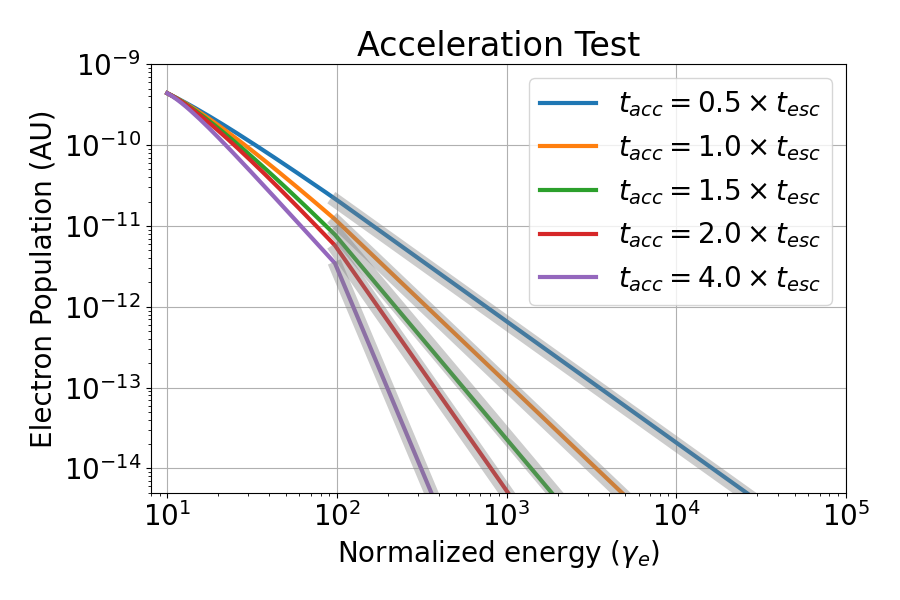
LABEL:Fig:Acceleration_Tests shows the result of the tests with different ratios of implemented by varying the value of . We obtain a near-exact match between the numerical curves and their theoretical values.
To test the cooling code, we take a similar approach to the acceleration test, but we inject electrons only at high energies with a power law index of . The first part of this test studies the behaviour of the particle population below the injection point. By assuming a simplified version of (LABEL:kinetic_equation) in which there is neither injection nor acceleration and the only losses are due to escape and cooling, we can obtain a steady state solution for the population as:
| (44) |
where is a constant. In the absence of other contributions to the particle population, this solution fully represents the particle population distribution below the lower cut-off of the injection. For values of , the exponential term tends to and we obtain the result that the population behaves like a power law with index . For other cases, the exponential term is important and causes an exponential drop in the population towards lower energies. Physically, the first case represents that the cooling timescale is lower than the escape timescale where particles cool faster than they escape, which gives the power law behaviour. In the second case, we have that particles can escape much faster than they cool, so the population drops exponentially towards lower energies.
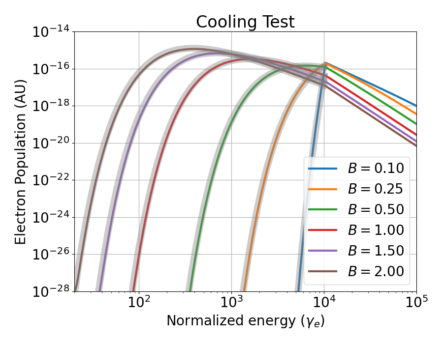
In 2 we show the resulting population of electrons for six different values of the magnetic field where on one extreme we have that the main driver of the particle population is escape, whereas for the other it is cooling. The bands follow (LABEL:population_low_energy_steady_state) with chosen as to match approximately the value of the population at the lower end of the injection point. As we can see, the match is quite good, which demonstrates the validity of our approach for the cooling algorithms.
The second part of the cooling test involves the behaviour of the particles in the injection range. For this range, we have again two behaviours depending on the cooling and escape timescales. The transition between these two behaviours is defined by a cooling break energy, which can be estimated as . Hence, keeping and constant, we can vary the value of the magnetic field to control the position of the cooling break. Below the cooling break, we have a population that is escape dominated, and develops into a population that keeps the original behaviour of the injection profile. Above the cooling break, the population is cooling dominated and as a result the population follows a power law steepened by .
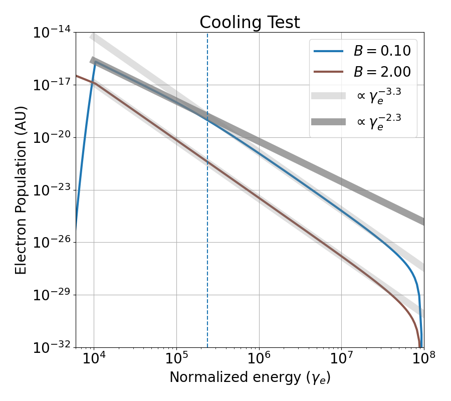
For 3 we have tested two values of the magnetic field . In the first case (blue line), the cooling break is between the injection ends, so we get two behaviours as expected. For the lower energy part, the resulting population has an index of and for the higher energy part, the index is , just as expected. Below the injection lower limit, the population of electrons escapes freely and that is reflected by the abrupt drop in population. For the second case (brown line), the cooling timescale is much lower and the cooling break is below the lower injection limit. Hence, between the injection ends, we see that the whole population has a index of .
In addition to the above tests, which are designed to stress the acceleration and cooling parts of our numerical schemes, we have also performed tests aimed towards checking the correctness of the implementation of the physical processes. In this case, we have checked that the tests of Dimitrakoudis et al. (2012) pass. Further demonstrations of the code can be found in Jiménez-Fernández & van Eerten (2020).
6 Bayesian Inference, Markov Chain Monte Carlo and Nested Sampling analysis
Bayesian inference provides a useful approach to parameter estimation and model selection. In this section we describe some of the key concepts of Bayesian inference and how it can be used in the task of fitting a model. For the case of blazar modelling, we additionally describe two different approaches that Katu is able to work with via two available wrappers: Markov Chain Monte Carlo (MCMC) analysis in the form of an ensemble sampler with affine invariance Goodman & Weare (2010) and Nested Sampling (NS) analysis in the form of nested elliptical sampling Feroz & Hobson (2008).
6.1 Bayesian Inference
We define a dataset as the combination of observations and their associated errors . A model is defined as some function that can be applied to a set of parameters to obtain some model predictions that can be compared with the dataset. Then, we can define the probability that a dataset has been obtained given a model and a set or parameters as:
| (45) |
where is called the likelihood. Likewise, we can also define the a priori probability, or belief, of the parameters that we have used:
| (46) |
where is denoted the prior. For example, when comparing leptonic and lepto-hadronic models, the parameter that most determines this division is . If we have any a priori information suggesting a certain distribution for , we can include this information as a prior. If not, the prior is typically set to be flat. Note however that this does not mean that no prior assumptions were included: a flat prior in logarithmic space will for example have a different impact than a flat prior in linear space.
By integrating over the whole parameter space , we can obtain the probability of obtaining a dataset given a model:
| (47) |
where is the evidence of the model, or, simplifying the notation:
| (48) |
The evidence can be understood as a weighted average of the likelihood over the whole parameter space with the prior as a weight function. Thus, only the regions where the product of both the likelihood and the prior is high will mainly contribute to the value of the evidence. By integrating over the whole parameter space with a normalized prior, we are implicitly dividing by the volume of the space so models with more parameters that do not improve the likelihood will obtain a lower evidence.
By applying Bayes’ theorem, we can find the probability of a model given a dataset:
| (49) |
where and are the a priori probability, or belief, of the model and the data respectively. Here, denotes the probability of measuring the dataset from the underlying physics and the observation method. encapsulates our prior belief in the model that is not already reflected in the priors of the parameters. For example, if we know that blazars could be fit from two different models with a ratio of to , we can incorporate this information in this term.
Denoting two models by and , we can take the ratio of their probabilities to obtain:
| (50) |
Assuming that both models have the same a priori probability, we are left with the ratio of evidences as a way of comparing two models, so that if model is more likely and vice versa, if , model is more likely.
As with all criteria for model selection, the actual amount of (relative) confidence in a given model that is linked to a given numerical value of R remains subjective. Taking as a guideline Kass & Raftery (1995), we give the following references for the value of : , ‘not worth more than a bare mention’; , ‘substantial’; , ‘strong’ and , ‘decisive’.
By inverting (LABEL:evidence_expanded) and the conditioning, we can find the probability of a point in parameter space given a dataset and a model:
| (51) |
which we call the posterior distribution of : . Simplifying the notation, we obtain:
| (52) |
For the purpose of parameter estimation, it is not necessary to compute the evidence.
Assuming that the data follow a Gaussian distribution, we can define the log-likelihood444The reader should not confuse the Likelihood with the log-likelihood . associated between a dataset and the model predictions as:
| (53) |
The first term is a constant for every log-likelihood, as it does not depend on the model, only on the errors of the data. It can be proven that this term appears as a constant multiplicative factor upon the calculation of the evidence, so it divides out when comparing the evidence of two models.
6.2 MCMC and Nested Sampling
MCMC and Nested Sampling are two different approaches to analyse, using bayesian inference, a model given its likelihood. MCMC can sample from a given function, which in this case it is the likelihood of the model, and thus, we can reconstruct the shape of the likelihood and the posterior probabilities of any of its parameters. Nested sampling works by sampling from the likelihood function in a monotonically increasingly way. By assigning a statistical weight to each of the samples, the shape of the likelihood can be reconstructed and the evidence of the model can be calculated.
Even though sampling using MCMC is simple in principle, it has some drawbacks when the shape of the sampled distribution has various maxima and/or is very different from a simple gaussian. In order to avoid partially these problems, Goodman & Weare (2010) introduce the ’Ensemble Samplers with Affine Invariance’ and Foreman-Mackey et al. (2013) creates, using ideas from that work, emcee. The MCMC steps introduced in Goodman & Weare (2010) and implemented in emcee allows for sampling efficiently from any distribution that can be reduced to a multivariate gaussian by an affine transformation, increasing greatly the distributions for which MCMC is efficient at the cost of increasing the memory requirements. In particular, whereas simple MCMC uses a ’walker’ to traverse the parameter space, emcee uses an ensemble of them.
Even though the affine invariant ensemble samplers and emcee are a great statistical tool, they still have some problems inherited from the basic MCMC analysis. First, MCMC tends to perform very badly in situations where multiple modes exist, as it can take a long time for a walker to go from one maximum to another because in its path there is a volume of likelihood that is taken with lower probability than other steps. Second, MCMC needs some period of burn-in until the sampler starts to produce samples that are independent and representative of the sampled probability distribution. Third, not every distribution is well represented by affine transformations of a multivariate gaussian, so there are cases where emcee will still perform not optimally.
Nevertheless, after some iterations, we obtain a chain of parameters for each walker from which we can derive the sought for posterior probabilities by simply plotting the appropiate histograms.
In contrast to MCMC analysis, nested sampled is aimed towards the calculation of the evidence. The basic idea is that, by creating a sequence of points with increasingly likelihood and by assigning a weight to each of them depending on their position in the sequence, the evidence can be calculated. As the value of the likelihood increases in the sequence, the probability of drawing a new point with a better value decreases. multinest avoids this problem by using a set of points as ’live points’ and using them to define ellipses from where to drawn the new points (Feroz et al., 2009). This way, the sampling is much more efficient and the sequence can grow faster.
As the set of ’live points’ define the sampled volume, it can happen that this volume can be separated into isolated sub-volumes. In these cases, each of the sub-volumes is associated with one maximum of the likelihood function, and Nested Sampling, and multinest by extension, can detect and handle these separated maxima with ease.
Even though the length of the sequence can be made as big as wanted, there is a point where the last points contribute very little to the calculation of the evidence. multinest, by default, is set to stop the calculation of the evidence when the best point of the sequence increases the value of the log evidence by less than some tolerance.
Each of the points in the sequence is assigned a weight, and thus, can be used to create the histograms of the posterior probabilities of the parameters.
7 Application to Mrk 421
7.1 Dataset
The blazar Markarian 421 (Mrk 421) has been observed for decades. Mrk 421 is one of the nearest blazars to earth, and therefore one of the brightest. Mrk 421 is a BL Lacertae object, which tend to be variable in their flux levels and can typically be modelled without a need for an external source of photons.
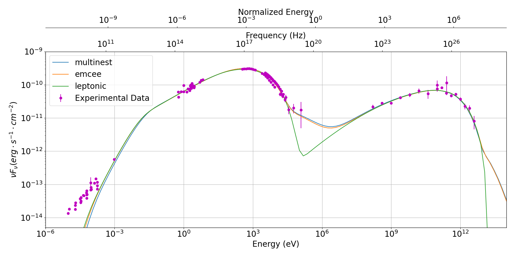
The full dataset that we study was gathered during a year long multi-wavelength campaing during 2009, whose details are reported on Abdo et al. (2011) and we reproduce it in 4. It is important to notice that not all the experimental points follow the same trend, even when taking into account their errors. As an example of this problem, we reproduce the X-rays part of the SED in 5, where it can be clearly seen that there are two different trends with the different instruments, Swift and RXTE, where the first shows a lower flux than the second.
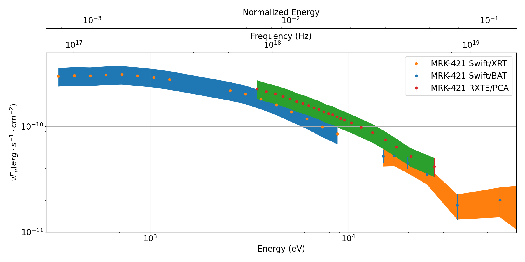
Similarly, observations at optical frequencies display a spectral variability that goes beyond their (very small) observational errors. To account for these systematic deviations from the base line physics captured by our model, we take a conservative approach to the sizes of the error bars of the observations (for an alternative approach when fitting complex models to broadband transient data, see Aksulu et al. (2020)). By increasing the error bars according to the prescription below, we acknowledge that our model fit is to the generic state of the blazar SED during the period of observation rather than to its instantaneous value at a given time of observation for a specific instrument. We use
| (54) |
where is the final error that we take, is a constant, is the experimental flux and is the experimental error. For this analysis, we have chosen to separate the value of by band and have set and . In 5 we show with bands the resulting error bands that we obtain and see that a common trend can be more easily fitted between the observations.
For the case of X-rays, the existence of two trends in the data had an important impact upon the fitting procedure and its results. The first consequence is that it creates two maxima in the likelihood function where each one is linked to each of the trends. The existence of more than one maximum can cause problems to fitting algorithms. For emcee, as we have discussed in 6.2, because it needs to have walkers in both maxima as it would be complicated for the walkers to go from one maxima to the other, and because in the degenerate case of having all walkers in one of the maxima the fitting procedure would need a very high time to ’discover’ the other maxima. For multinest the multiples maxima are not such a serious problem as it has the capability of discovering, separating and analysing each of the maxima separately, although in some cases, depending on the shape of the likelihood function this is not easy, or even doable. In both cases, what we would find is that the running time and the acceptance ratio of the fitting algorithms would be very high and low respectively.
The flux detected by SMA and most of the radio observatories should be handled carefully as they can not resolve the jet and instead detect the integrated flux from the galaxy. To take this into account, we have chosen to use the SMA point as an upper limit in our fits. Upper limits can be treated in different ways in a model fit. In this case, we have chosen to discard all model-generated SEDs that led to flux levels above the SMA value. Because the SMA upper limit in practice then automatically forces the SED to go below the radio upper limits at longer wavelengths, we can safely omit these from our fitting process without changing the outcome (confirmation of this is provided in 7.3).
7.2 Configuration
As we have discussed in 4 and can be seen in B, Katu supports a high number of configuration options. To focus on one particular set of models, we choose to set the plasma volume to a sphere and to allow for all the particles to evolve. Additionally, all the initial population distributions have ben set to simple power laws.
The background density and its ratio of protons to electrons has been set to and respectively. Note that these values have no reflection on the final steady state, as the initial distribution will be overwhelmed by the injected one.
For the electrons, we have chosen a lower cut-off for the energy range of and higher cut-off of , where and are the values of the upper cut-offs of the electron and proton injection distributions respectively. These limits allow that electrons can cool down to very low energies and that all the electrons that are produced through photo-meson and the Bethe-Heitler processes can be injected in the distribution.
Photons are also produced by many processes, so their energy limits have to be chosen to reflect this. We have taken a lower cut-off of and a higher cutoff of , which is the value of the higher energy cut-off for the electrons. We have also chosen to not inject photons from the exterior of the volume, so we set the value of the photon luminosity as .
For protons, we have taken that both, the initial and the injection distribution have the same shape, with a lower cut-off value of , a higher cut-off value of and a power law index of .
We assume that the charged particles scape slower than neutral particles, so we have set the charged to free escape ratio as .
Even though we do not know of any process that would preferentially accelerate one kind of particle over the other, we have chosen to set the ratio of protons to electrons as a free variable to further explore the hadronic capabilities of our model. In 7.4 we fix this ratio to in order to have virtually no protons and thus, be able to simulate a fully leptonic model.
Numerically, we have chosen to set the tolerance to and have set the number of bins for the primary particles as: and . Experience shows that these settings provide a good balance between numerical accuracy and reasonable convergence times for the simulations.
Finally, we are left with free variables, which are gathered in 2, along with the respective search ranges. , and correspond to the parameters of the injected population of electrons. and are the magnetic field and the Doppler boosting parameter of the volume, respectively; is the radius of the sphere we simulate; and and correspond to the total luminosity of the injected particles (in the plasma frame) and its ratio of protons to electrons. As cosmological parameters, we have chosen those of Collaboration et al. (2019): , and .
| Parameter | Search Range |
|---|---|
7.3 Results
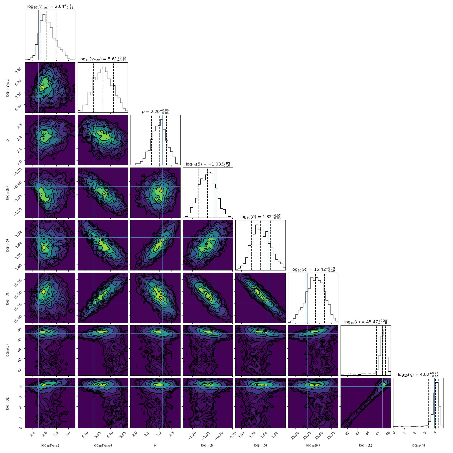
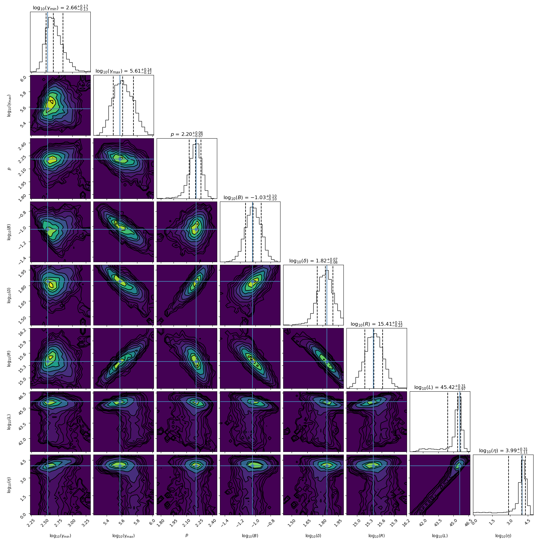
The results of the two statistical packages that we have tested are presented in 3 and 4. The corresponding corner plots for both packages can be seen in LABEL:fig:[s]Corner-Plot-multinestand 7 respectively.
| Parameter | multinest | emcee | ||
|---|---|---|---|---|
| Best | Median | Best | Median | |
It can be clearly seen from 3 that both approaches give very similar results for the best parameters, the median and the and percentiles, which show the consistency of the analysis of both packages. Likewise, from both corner plots, LABEL:fig:[s]Corner-Plot-multinestand 7, we see that the posterior shape and the 2D correlations are consistent. Furthermore, we see in 4 that both SEDs are very close together, and indeed, their log likelihoods are and for multinest and emcee, respectively. For multinest, we can also quote the value of the log evidence, which is not available for emcee, .
The choice that we made in 7.1, namely to choose the SMA datapoint as an upper limit and ignore the rest of the radio detections on the basis that the SMA was the most restricting one, is correct, as none of the best fits of the SED go above any of the radio datapoints.
In computational terms, it is complicated to compare both algorithms due to how they handle points with null likelihood, as multinest silently discards them while emcee treats them as any other point; and how the first steps of emcee had been handled. multinest has taken about a day of computations and at least on the order of evaluations of the log likelihood function, whereas emcee has taken more than evaluations and more than double the time, although part of these evaluations were done in initial short runs and due to leaving emcee to work overnight without a clear stopping condition.555All the computations were done on a server with 32 available cores with multinest and emcee calculating 8 log likelihoods in parallel and Katu with 4 threads. Even though emcee seems worse from the point of view of finishing the runs, it tends to give a result for the best log likelihood much sooner, and usually better, than multinest.
From 4, it can be seen that in the range of eV, there is a small hump between the synchrotron and inverse Compton peaks. In our simulations, this is caused by the pairs created by the Bethe-Heitler process Mastichiadis et al. (2005); Petropoulou & Mastichiadis (2015), highlighting the need for protons in order to completely fit the SED.
Abdo et al. (2011) estimate the luminosity of the blazar between and . Taking that the luminosity from the jet frame to the blazar frame transforms as , we obtain and . Both values are clearly above the estimation of Abdo et al. (2011), an issue shared with other lepto hadronic models Liodakis & Petropoulou (2020).
7.4 Model selection using Bayesian inference: leptonic versus lepto-hadronic models
To verify that the small hump that appears between the peaks in 4 is indeed caused by the presence of protons and to compare our results against a purely leptonic model, we choose to repeat the statistical analysis of Mrk 421’s data with multinest but setting . This ratio of injected protons to electrons means that, effectively, the hadronic processes have no impact upon the final fit. The choice of multinest over emcee is to allow us to obtain a value for the evidence that we can compare against the evidence for the hadronic model.
As we can see in 4, the best SED that the leptonic model can produce is unable to fit the high energy part of the X-ray observations, and this is indeed reflected in the best log likelihood that it can achieve: . We also find that the log evidence has a value of .
Assuming that both models have the same a priori probability, we find that the hadronic model is favoured as:
The corresponding Bayes’ Factor is . This value is consistent with the qualification substantial for the evidence in favour of the lepto-hadronic model, as discussed in 6.1. Note that this measure already accounts for the different number of parameters between the two models.
Lepto-hadronic models can successfully explain some of the features of blazar SEDs, such as the gamma ray peak being caused by neutral pion decay or proton synchrotron Mannheim (1993); Cerruti et al. (2015). But, leptonic models can also fit this peak with inverse compton scattering of synchrotron photons, and the energy requirements for the proton population are usually above the Eddington luminosity Liodakis & Petropoulou (2020). Some characteristics of the SEDs can only be explained by a hadronic population, such as a population of pairs produced by the Bethe-Heitler pair production process, or the presence of neutrinos Mastichiadis et al. (2005); Petropoulou & Mastichiadis (2015); Petropoulou et al. (2015); Rodrigues (2019); Rodrigues et al. (2020). However, to our knowledge, this is the first time that the dichotomy of leptonic vs. lepto-hadronic modelling has been explored from a fully bayesian point of view using kinetic equation modelling.
8 Summary
In this work we introduce the code Katu, for simulating the evolution of plasmas according to a set of kinetic equation for a series of particles. We have tried to capture as much of the physics as possible by adding diverse processes in a detailed way. We have tried to make it as performant as possible, on the mathematical front by adapting the kinetic equation to the species of particle and separating neutral from charged particles, and on the computational front by takind advantage of multi-threading and by calculating as much as possible up-front.
Given that Katu is fast, we are able to tie it to two commonly used statistical packages that can perform bayesian analysis of models, emcee and multinest. emcee is a python package that performs bayesian analysis by using affine invariant samplers for MCMC and multinest is a Fortran package, which we employ using pymultinest, which implements Elliptical Nested Sampling.
As an example of its usage, we show how Katu and both wrappers can be used to analyse the well known blazar Mrk 421 obtaining, as expected, that both statistical packages report similar values for the best, median and and percentiles of the posterior of the parameters.
Additionally, we perform the test of exploring a purely leptonic model, finding that there is substantial evidence to reject it in favour of a lepto-hadronic model.
The code Katu was also employed for the study of TXS 0506+056, as described in Jiménez-Fernández & van Eerten (2020).
Acknowledgements
The authors would like to thank Matteo Cerruti and Anatoli Fedynitch for the valuable discussions about their models and Petar Mimica for hosting them during their meetings at the University of Valencia. B.J.F. would also like to thank the late Cosmo the Cat, Jinx, Loki and Mina the Cats and Lottie the Dog for their support. B.J.F. acknowledges funding from STFC through the joint STFC-IAC scholarship program. H.J.v.E. acknowledges partial support by the European Union Horizon 2020 Programme under the AHEAD2020 project (grant agreement number 871158).
References
- Abdo et al. (2011) Abdo A. A., et al., 2011, The Astrophysical Journal, 736, 131
- Aksulu et al. (2020) Aksulu M. D., Wijers R. A. M. J., van Eerten H. J., van der Horst A. J., 2020, Monthly Notices of the Royal Astronomical Society, 497, 4672
- Blumenthal (1970) Blumenthal G. R., 1970, Physical Review D, 1, 1596
- Böttcher & Schlickeiser (1997) Böttcher M., Schlickeiser R., 1997, Astronomy & Astrophysics, p. 5
- Böttcher et al. (2012) Böttcher M., Harris D. E., Krawczynski H., 2012, Relativistic Jets from Active Galactic Nuclei
- Cerruti et al. (2015) Cerruti M., Zech A., Boisson C., Inoue S., 2015, Monthly Notices of the Royal Astronomical Society, 448, 910
- Collaboration et al. (2019) Collaboration P., et al., 2019, arXiv:1807.06209 [astro-ph]
- Crusius & Schlickeiser (1986) Crusius A., Schlickeiser R., 1986, Astronomy & Astrophysics, 164, L16
- Dimitrakoudis et al. (2012) Dimitrakoudis S., Mastichiadis A., Protheroe R. J., Reimer A., 2012, Astronomy & Astrophysics, 546, A120
- Feroz & Hobson (2008) Feroz F., Hobson M. P., 2008, Monthly Notices of the Royal Astronomical Society, 384, 449
- Feroz et al. (2009) Feroz F., Hobson M. P., Bridges M., 2009, Monthly Notices of the Royal Astronomical Society, 398, 1601
- Feroz et al. (2013) Feroz F., Hobson M. P., Cameron E., Pettitt A. N., 2013, arXiv:1306.2144 [astro-ph, physics:physics, stat]
- Foreman-Mackey et al. (2013) Foreman-Mackey D., Hogg D. W., Lang D., Goodman J., 2013, Publications of the Astronomical Society of the Pacific, 125, 306
- Gao et al. (2017) Gao S., Pohl M., Winter W., 2017, The Astrophysical Journal, 843, 109
- Gao et al. (2019) Gao S., Fedynitch A., Winter W., Pohl M., 2019, Nature Astronomy, 3, 88
- Ghisellini (2013) Ghisellini G., 2013, arXiv:1202.5949 [astro-ph 10.1007/978-3-319-00612-3, 873
- Goodman & Weare (2010) Goodman J., Weare J., 2010, Communications in Applied Mathematics and Computational Science, 5, 65
- Hümmer et al. (2010) Hümmer S., Rüger M., Spanier F., Winter W., 2010, The Astrophysical Journal, 721, 630
- Jiménez-Fernández & van Eerten (2020) Jiménez-Fernández B., van Eerten H. J., 2020, Monthly Notices of the Royal Astronomical Society, 500, 3613
- Jones (1968) Jones F. C., 1968, Physical Review, 167, 1159
- Kass & Raftery (1995) Kass R. E., Raftery A. E., 1995, Journal of the American Statistical Association, 90, 773
- Keivani et al. (2018) Keivani A., et al., 2018, The Astrophysical Journal, 864, 84
- Kelner & Aharonian (2008) Kelner S. R., Aharonian F. A., 2008, Physical Review D, 78
- Lightman & Zdziarski (1987) Lightman A. P., Zdziarski A. A., 1987, The Astrophysical Journal, 319, 643
- Liodakis & Petropoulou (2020) Liodakis I., Petropoulou M., 2020, The Astrophysical Journal, 893, L20
- Lipari et al. (2007) Lipari P., Lusignoli M., Meloni D., 2007, Physical Review D, 75
- Mannheim (1993) Mannheim K., 1993, arXiv:astro-ph/9302006
- Mastichiadis & Kirk (1992) Mastichiadis A., Kirk J. G., 1992, Nature, 360, 135
- Mastichiadis & Kirk (1995) Mastichiadis A., Kirk J. G., 1995, Astronomy & Astrophysics, 295, 613
- Mastichiadis et al. (2005) Mastichiadis A., Protheroe R. J., Kirk J. G., 2005, Astronomy & Astrophysics, 433, 765
- Petropoulou & Mastichiadis (2015) Petropoulou M., Mastichiadis A., 2015, Monthly Notices of the Royal Astronomical Society, 447, 36
- Petropoulou et al. (2015) Petropoulou M., Dimitrakoudis S., Padovani P., Mastichiadis A., Resconi E., 2015, Monthly Notices of the Royal Astronomical Society, 448, 2412
- Petropoulou et al. (2020) Petropoulou M., Oikonomou F., Mastichiadis A., Murase K., Padovani P., Vasilopoulos G., Giommi P., 2020, The Astrophysical Journal, 899, 113
- Rodrigues (2019) Rodrigues X., 2019, PhD thesis, Humboldt University, https://ui.adsabs.harvard.edu/abs/2019PhDT........87R/abstract
- Rodrigues et al. (2020) Rodrigues X., Garrappa S., Gao S., Paliya V. S., Franckowiak A., Winter W., 2020, arXiv:2009.04026 [astro-ph]
- Rybicki & Lightman (1979) Rybicki G. B., Lightman A. P., 1979, Radiative processes in astrophysics. Wiley, New York
- Svensson (1982) Svensson R., 1982, The Astrophysical Journal, 258, 321
Appendix A Detailed Description of the processes
In this appendix we try to give a detailed description of the equations that we implement in our model, along with the references. The reader must notice two things. First, we have adapted the notation to make it consistent with our conventions through the text. Additionally, some equations have been rearranged into equivalent forms that are a bit simpler. Second, our numerical implementation, even though it follows these equations as closely as possible, has some quirks that the reader and anyone implementing the model should be aware of.
Note also that we do not explicitly add anything about the losses of particles due to decay because this term is explicitly tracked in the kinetic equation, 1.
In the first place, some of the equations are physically valid in limits such as , , , etc. but numerically they either become unstable or they fall into regimes where ’catastrophic loss of precision’ could happen. In these cases, the special cases have been pulled out and are treated separately or are accounted for by using approximations.
In the second case, in general, the integrals are taken in logarithmic space in energy, as that makes the bins equally sized and in general the energy term that is introduced can be simplified, which also simplifies the equations. Numerically, they are performed using the trapezium rule, which gives a good precision taking into account the errors already introduced by the approximations in the models and the final data we compare with. Likewise, the derivatives are calculated using a first order scheme, although in log-log space, as they are much more stable this way.
A.1 Synchrotron Emission and Absorption
In our model, all the charged particles create synchrotron emission, have synchrotron losses and cause synchrotron absorption. For this, we model the emission as:
| (55) |
where is the energy emitted by a particle with energy at frequency and has the form (Crusius & Schlickeiser, 1986):
| (56) |
where and are the charge and the mass of the emitting particle, is the magnetic field strength, is the frequency normalized to a critical frequency with
| (57) |
and is a function given in terms of Whittaker functions:
| (58) |
The loss of energy of the emitting particles is modelled as:
| (59) |
where is the Thomson cross-section and is the energy density of the magnetic field.
The absorption of photons is modelled as:
| (60) |
A.2 Inverse Compton
Photons interact with energetic electrons due to the inverse Compton process, which we model as:
| (61) |
where is the initial energy of the photon, is the energy after the scattering, is the electron population, is the photon population and are two functions referring to the upscattering and downscattering of photons which where calculated by Jones (Jones, 1968, equations 40 and 44):
| (62) | ||||
| (63) |
with
| (64) |
The loss term for photons can be obtained as:
| (65) |
where is the reaction rate of electrons of energy with photons of energy and can be found from integrating the Klein-Nishina cross section.
| (66) |
where:
| (67) |
and the dilogarithm.
Following Böttcher et al. (2012), we use the simplified prescription for the electron energy losses in inverse Compton scattering:
| (68) |
where is the energy density of the photon field:
| (69) |
A.3 Two photon Pair Production
Photons can interact among themselves creating electron and positron pairs, which we model according to (Böttcher & Schlickeiser, 1997).
Let us define
| (70) | ||||||
| (71) |
where are the energies of the initial photons and is the energy of the final electron or positron.
Then we can obtain the rate of created particles as:
| (72) |
where
| (73) |
The values for are given by energetic and kinematic reasoning:
| (74) |
where
| (75) |
The function is given depending on the value of :
| (76) |
with
| (77) |
Photon losses are modelled according to the fully integrated cross section in a similar way to the photon loss term for IC.
| (78) |
where and .
A.4 Pair Annihilation
Just like a pair of photons can interact to produce a pair electron-positron, the opposite process can happen where electrons and positrons annihilate among themselves to produce a pair of photons. We model this process following Svensson (1982).
Let us start by defining the auxiliary variables:
| (79) | ||||||
| (80) |
note that these definitions are similar but different to the case of pair production. In particular, and go with not the other way around.
Svensson (1982) defines the spectral emissivity as:
| (81) |
where is the angle averaged emissivity and the limits and are defined using the auxiliary functions:
| (82) | ||||||
| (83) |
which give the integration limits as:
| (84) | ||||||
| (85) | ||||||
The angle averaged emissivity is given by:
| (86) |
where the limits are given by kinetic reasoning:
| (87) | ||||||
| (88) | ||||||
The is given again in a form that depends on whether is equal or different from .
| (89) |
where
| (90) |
A.5 Photo-Meson Production
Hadrons (protons and neutrons) interact with photons producing hadronic resonances which ultimately decay in the form of hadrons and pions. To model this we follow the approximations of Hümmer et al (Hümmer et al., 2010) in their SimB model. We diverge though in the calculations of the loss and self-injection term for hadrons as, instead of applying a cooling term, we model every process as a loss and where applicable, we reinject the corresponding hadron with reduced energies.
For this process, and in order to avoid adding constants and units we choose to follow the original convention on units and notation. We begin with the equation for the injection of particles from an interaction between a photon and a proton:
| (91) |
where makes reference to the Interaction Type and to the daughter particle. The constants , and and the function depend on the interaction type.
For the Resonant Pion production, we follow their Simplified Model B (Hümmer et al., 2010, section 4.2.2 & Table 4), whose parameters we reproduce in 4.
| IT | Range (GeV) | (barn) | Initial Proton | Initial Neutron | K | ||||||
| LR | |||||||||||
| HR | |||||||||||
The functions are given depending on the Interaction Type as:
| (92) |
| (93) |
For the direct pion production, we follow (Hümmer et al., 2010, section 4.3 & Table 5), whose parameters we reproduce in 5.
| IT | (GeV) | (GeV) | K | Initial Proton | Initial Neutron | |||||
The functions are given by;
| (94) |
The functions are parametrized in terms of and are different depending on the interaction type:
| (95) |
| (96) |
For the multi pion production, we follow (Hümmer et al., 2010, section 4.4.2 & Table 6), whose parameters we reproduce in 6.
| IT | (GeV) | (GeV) | K | Initial Proton | Initial Neutron | ||||||
|---|---|---|---|---|---|---|---|---|---|---|---|
| 0.5 | 0.9 | 60 | 0.1 | 0.27 | 0.32 | 0.34 | 0.04 | 0.32 | 0.04 | 0.34 | |
| 0.5 | 0.9 | 60 | 0.4 | 0.17 | 0.29 | 0.05 | 0.17 | 0.05 | 0.29 | ||
| 0.9 | 1.5 | 85 | 0.15 | 0.34 | 0.42 | 0.31 | 0.07 | 0.42 | 0.07 | 0.31 | |
| 0.9 | 1.5 | 85 | 0.35 | 0.19 | 0.35 | 0.08 | 0.19 | 0.08 | 0.35 | ||
| 1.5 | 5.0 | 120 | 0.15 | 0.39 | 0.59 | 0.57 | 0.30 | 0.59 | 0.30 | 0.57 | |
| 1.5 | 5.0 | 120 | 0.35 | 0.16 | 0.21 | 0.13 | 0.16 | 0.13 | 0.21 | ||
| 5.0 | 50 | 120 | 0.07 | 0.49 | 1.38 | 1.37 | 1.11 | 1.38 | 1.11 | 1.37 | |
| 5.0 | 50 | 120 | 0.35 | 0.16 | 0.25 | 0.23 | 0.16 | 0.23 | 0.25 | ||
| 50 | 500 | 120 | 0.02 | 0.45 | 3.01 | 2.86 | 2.64 | 3.01 | 2.64 | 2.86 | |
| 50 | 500 | 120 | 0.5 | 0.20 | 0.21 | 0.14 | 0.20 | 0.14 | 0.21 | ||
| 500 | 5000 | 120 | 0.007 | 0.44 | 5.13 | 4.68 | 4.57 | 5.13 | 4.57 | 4.68 | |
| 500 | 5000 | 120 | 0.5 | 0.27 | 0.29 | 0.12 | 0.27 | 0.12 | 0.29 | ||
| 5000 | 120 | 0.002 | 0.44 | 7.59 | 6.80 | 6.65 | 7.59 | 6.65 | 6.80 | ||
| 5000 | 120 | 0.6 | 0.26 | 0.27 | 0.13 | 0.26 | 0.13 | 0.27 | |||
The functions are given by;
| (97) |
To account for energy losses in protons and neutrons, we also follow Hümmer et al. (2010, Appendix B), although we apply the framework of reinjection to all the particles and we ignore cooling. This way, all the losses can be treated with the same equation:
| (98) |
where is the resulting hadron and is the inelasticity of the interaction type and the corresponding channel.
A.6 Bethe-Heitler Process
Besides producing mesons, a photon interacting with a proton can produce pairs electron-positron through the Bethe-Heitler process. We have chosen to model this process using the results of Kelner & Aharonian (2008, Section IV).
First, the injection of produced particles is defined as:
| (99) |
where is the energy of the final electron (or correspondingly positron), is the energy of the initial proton and is the energy of the incoming photon. and act as integration variables which act as energies in the rest frame of the proton. Note that we have added a factor with respect to the original equation to correct the units.
In the limit of highly energetic protons we have that:
| (100) |
is the differential reaction rate:
| (101) |
which is available in Blumenthal (1970, equation 10) under de assumption of having a proton with infinite mass:
| (102) | ||||
where
| (103) | ||||||
| (104) | ||||||
| (105) | ||||||
and is the fine structure constant, is the electric charge of the scattering nucleus (in our case for protons ) and is the classical radius of the electron. We have chosen to keep the notation compact to denote the modulus of the momentum of a particle. Under the assumption of the proton having infinite mass, or being at rest, we have that .
We will focus on the second and third integrals, which only depend on external variables:
| (106) |
Pulling out some constants we obtain:
| (107) | ||||
| (108) | ||||
| (109) | ||||
| (110) | ||||
| (111) | ||||
| (112) |
As far as we know, no simple form for these integrals exist so they are performed numerically using an adaptive integration procedure from the Gnu Scientific Library.
Finally, to calculate the injection rate for electrons or positrons, (LABEL:BH_dne/dgp) has to be integrated over the proton population:
| (113) |
A.7 Pion-Muon Decays
To account for the cascade of pion and muon decays we follow the same model of Lipari et al. (2007) and Hümmer et al. (2010).
The injection of produced particles can be factorized as:
| (114) |
where and are the energies of the parent and daughter particles (not normalized), is the decay timescale of the parent particle and is a function that gives the ratio of decaying.
Charged pions decay to muons, which subsequently decay through the following channels:
The rate of charged pions decaying into neutrinos is given by Lipari et al. (2007):
| (115) |
For the decay into muons we need to track the helicity of the final muons, as it will impact the subsequent decays into neutrinos, Hümmer et al. (2010):
| (116) | ||||
| (117) |
Then, decay of muons to neutrinos is given by Hümmer et al. (2010):
| (118) | ||||
| (119) |
with for right handed muons and for left handed muons.
The functions that govern the subsequent injection of electrons and positrons do depend on the helicity of the parent muons and can be simplified to:
| (120) | ||||
| (121) |
A.8 Neutral Pion Decay
The injection of photons from neutral pions follows the simple equation:
| (122) |
Appendix B Configuration File
Katu is very easy to configure, this is done is done with the Toml666https://toml.io/en/ language, which allows us to separate variables per tables and subtables. An example configuration can be found in the default.toml file. As a reference, we detail all the possible options here.
The [general] table refers to general options for the simulation and the plasma. The possible keys are:
-
•
density: The density of the background plasma
-
•
magnetic_field: The magnitude of the background magnetic field
-
•
eta: The ratio of protons to electrons in the background plasma
-
•
cfe_ratio: The ratio of charged to free escape
-
•
t_acc: The acceleration timescale
-
•
dt: The initial value of the time step
-
•
dt_max: The maximum value of the time step
-
•
t_max: The maximum simulation time
-
•
tol: The requested tolerance for the steady state
The [volume] table refers to options referred to the shape of the simulation volume.
-
•
shape: The shape of the volume, currently it supports "sphere" and "disk"
-
•
R: The radius of the volume
-
•
h: The height of the disk. (Only used for the "disk" shape)
The external_injection table refers to the injection of particles from outside the simulated volume. The possible keys are:
-
•
luminosity: The integrated luminosity of the injected particles
-
•
eta: The ratio of protons to electrons to inject.
Note that the subtable external_injection.photons also has luminosity as a key separated from the particle injection.
The distribution tables and subtables ([protons], [electrons] and [photons]) refer to the distribution of particles, their limits and number of bins. The available keys are:
-
•
gamma_min: The minimum value for gamma for protons and electrons
-
•
gamma_max: The maximum value for gamma for protons and electrons
-
•
epsilon_min: The minimum value for epsilon for photons
-
•
epsilon_max: The maximum value for epsilon for photons
-
•
size: The number of bins for the particle kind
The distribution of the corresponding particle is controlled by the key distribution_type and supports the following options, along with the corresponding keys:
-
•
"maxwell_juttner": This option gives a thermal distribution of particles
-
–
temperature: The temperature of the distribution, in terms of the rest mass energy of the particle
-
–
-
•
"black_body": This option gives a thermal distribution of photons
-
–
temperature: The temperature of the distribution, in terms of the rest mass energy of an electron
-
–
-
•
"power_law": This option gives a simple power law
-
–
slope: The value of the exponent of the power law
-
–
-
•
"broken_power_law": This option gives a broken power law
-
–
break_point: The value of the energy where the the power law changes from the first slope to the second
-
–
first_slope: The value of the first exponent of the power law
-
–
second_slope: The value of the second exponent of the power law
-
–
-
•
"connected_power_law": This option gives a smooth power law with two slopes
-
–
connection_point: The value of the energy where the the power law changes from the first slope to the second
-
–
first_slope: The value of the first exponent of the power law
-
–
second_slope: The value of the second exponent of the power law
-
–
-
•
"power_law_with_exponential_cutoff": This option gives a power law with an exponential cutoff
-
–
slope: The value of the exponent of the power law
-
–
break_point: The normalization value for the energy in the exponential cutoff
-
–
-
•
"hybrid": This option gives a thermal distribution of particles at low energies coupled with a power law at higher energies
-
–
temperature: The temperature of the distribution, in terms of the rest mass energy
-
–
slope: The value of the exponent of the power law
-
–
Appendix C Corner Plots