Keck/KPIC Emission Spectroscopy of WASP-33b
Abstract
We present Keck/KPIC high-resolution () -band thermal emission spectroscopy of the ultra-hot Jupiter WASP-33b. The use of KPIC’s single-mode fibers greatly improves both blaze and line-spread stabilities relative to slit spectrographs, enhancing the cross-correlation detection strength. We retrieve the dayside emission spectrum with a nested sampling pipeline which fits for orbital parameters, the atmospheric pressure-temperature profile, and molecular abundances.We strongly detect the thermally-inverted dayside and measure mass-mixing ratios for CO (), H2O () and OH (), suggesting near-complete dayside photodissociation of H2O. The retrieved abundances suggest a carbon- and possibly metal-enriched atmosphere, with a gas-phase C/O ratio of , consistent with the accretion of high-metallicity gas near the CO2 snow line and post-disk migration or with accretion between the soot and H2O snow lines. We also find tentative evidence for , consistent with values expected in protoplanetary disks, as well as tentative evidence for a metal-enriched atmosphere (2–15 solar). These observations demonstrate KPIC’s ability to characterize close-in planets and the utility of KPIC’s improved instrumental stability for cross-correlation techniques.
1 Introduction
While large surveys have started to provide population-level insight into the physical and orbital properties of exoplanet systems, the details of exoplanet atmospheres, including composition, formation history, and 3D thermal structure, remain uncertain, with known trends suggesting substantial diversity (Mansfield et al., 2021). Improved knowledge of hot Jupiter atmospheres in particular may be a key piece to understanding the process of giant planet formation. Different formation scenarios are expected to produce differences in both relative atmospheric abundances (e.g. Öberg et al., 2011; Booth et al., 2017) and/or overall metallicity (e.g. Espinoza et al., 2017; Madhusudhan et al., 2017; Cridland et al., 2019). Recent observations (Pelletier et al., 2021; Line et al., 2021) have retrieved abundances which appear to conflict with the predictions from some of these theories, particularly the expectation of an inverse correlation between metallicity and C/O ratio (Espinoza et al., 2017; Cridland et al., 2019). These abundances may be explained by pebble drift (Booth et al., 2017), but these discrepancies suggest our understanding of either the planet formation process or atmospheric retrievals may be substantially incomplete.
Ultra-hot Jupiters (UHJs), with equilibrium temperatures , are a particularly interesting case for understanding planet formation processes.Two of the three hottest-known UHJs, KELT-9b and WASP-33b, orbit A-type stars on significantly misaligned orbits (Gaudi et al., 2017; Collier Cameron et al., 2010), suggesting a dynamical history of eccentric Kozai-Lidov effects (Naoz et al., 2011), though no additional planets are currently known in either system. Several A/B-type stars (e.g. HR 8799, Pic) have been found to host one or more massive planets on wide orbits, raising the possibility that UHJs are an alternative evolutionary outcome of such systems. UHJ atmospheres may thus hold indications of when and how planet migration occurred.
Understanding the formation of UHJs will also require understanding their extreme atmospheric chemistry. Commonly-used chemical equilibrium assumptions are expected to fail in the case of UHJs, particularly on the dayside, where extreme UV fluxes are expected to produce thermal inversions, drive mass loss, dissociate molecules, and even ionize some transition metals (Wyttenbach et al., 2020; Fu et al., 2022; Yan et al., 2021; Nugroho et al., 2021; Casasayas-Barris et al., 2019). These effects must be incorporated into 3D models in order to accurately model global energy transport (e.g. Roth et al., 2021). Transitions in phase/ionization state are expected on the nightside, when UV fluxes decline, though this will depend on the details of thermal redistribution between the hemispheres. Indications of rainout have been reported from analyses of transit observations of some UHJs (Ehrenreich et al., 2020; Wardenier et al., 2021; Johnson et al., 2023), but such observations have difficulty in unambiguously localizing a signal to a particular longitudinal range due to the complexity of 3D atmospheric circulation (Savel et al., 2022). Even the possibilities of photodissociation and rainout processes suggest current global circulation models (GCMs) coupled to a chemical-equilibrium radiative transfer framework are inadequate for modeling UHJ atmospheres, though understanding the modes of these failures and when they occur will require additional observational constraints (Pluriel et al., 2022). Understanding such modeling issues is critical for successfully interpreting chemical abundances as indicators of planetary formation and evolutionary history.
Recent advances in both analysis techniques and instrumentation have positioned high-resolution cross-correlation spectroscopy (HRCCS) as a promising method for obtaining constraints on the thermal and chemical properties of hot Jupiter atmospheres. This technique uses the change in the radial velocity of a close-in planet over several hours to isolate velocity-variable planetary spectral features from quasi-fixed stellar features using a cross-correlation (CC) template believed to match the planet and previously known orbital properties. Initially used to detect molecules such as CO and H2O in hot Jupiter atmospheres (e.g. Snellen et al., 2010; Brogi et al., 2012; Lockwood et al., 2014; Buzard et al., 2020), Brogi & Line (2019) developed a log-likelihood (logL) function that enables Bayesian retrievals of high-resolution observations, using forward models to produce CC templates which better match observations. Using this approach, Pelletier et al. (2021) retrieved a CO abundance and pressure-temperature (PT) profile for the hot Jupiter Boo A b, and Line et al. (2021) were able to retrieve both CO and H2O abundances for WASP-77A b, yielding the first robust C/O ratio measurement for an unresolved planetary companion from high-resolution spectroscopy. Key to these retrievals are fast radiative transfer tools, which can quickly produce high-resolution spectra for planets with arbitrary molecular abundances and PT profiles, obviating assumptions about atmospheric chemistry or bulk composition.
Concurrent with these improvements in data analysis, new instruments are being developed and deployed with design features better suited for CC-based techniques than previous facilities. In particular, Rasmussen et al. (2021) identified correlated noise and minor blaze function variations as having major impacts on the final detection strength when using these techniques, which can be improved by using highly stable instruments. The use of single-mode fibers (SMFs) in Keck/KPIC (Delorme et al., 2021) accomplishes this for the NIRSPEC (McLean et al., 1998; Martin et al., 2018; López et al., 2020) high-resolution () spectrograph on Keck. While the the Keck AO system and fiber coupling losses reduce overall throughput by a factor of compared with a seeing-limited slit spectrograph in KPIC phase I (Delorme et al., 2021), the SMFs offer an ultra-stable line-spread function, as well as improvements in the blaze function and wavelength solution stabilities (though systematics may persist below the level, well below the NIRSPEC resolution). Our analysis of KPIC phase I data showed no indications of intra-night variations in either the blaze function or wavelength solution. While Finnerty et al. (2022) reported no apparent variation at the level in the KPIC LSF over phase I, KPIC suffers from a time-varying fringing effect which must be corrected (see Section 3), caused by interference between two pickoff dichroics (Finnerty et al., 2022). KPIC is a prototype instrument with ongoing hardware upgrades, which will correct this in the future.
In this paper, we present Keck/KPIC phase I observations of the UHJ WASP-33b covering the dayside hemisphere. We use a free-retrieval approach to recover orbital velocity parameters, chemical abundances, and pressure-temperature (PT) profiles. Section 2.1 presents properties of the system and previous results for atmospheric characterization of WASP-33b, followed by a presentation of our KPIC observations in Section 2.2. We discuss our retrieval procedure and choice of parameters/priors in Section 3, including a verification of our retrieval setup using simulated datasets with known inputs. The results of our retrievals for WASP-33b are presented in Section 4. We discuss these results in the context of previous studies of UHJ atmospheres and planet formation predictions in Section 5. Section 6 summarizes our results.
2 Observations and Data Reduction
2.1 Target Properties
| Property | Value | Ref. |
|---|---|---|
| WASP-33 | ||
| RA | 02:26:51.06 | Gaia Collaboration (2020) |
| Dec | +37:33:01.7 | Gaia Collaboration (2020) |
| Spectral Type | A5 | Grenier et al. (1999) |
| 7.47 | Cutri et al. (2003) | |
| Mass | 1.495 | Collier Cameron et al. (2010) |
| Radius | 1.44 | Collier Cameron et al. (2010) |
| Teff | 7400 K | Collier Cameron et al. (2010) |
| 86.6 | Johnson et al. (2015) | |
| -9.2 | Gontcharov (2006) | |
| Age | Myr | Collier Cameron et al. (2010) |
| +0.1 dex | Collier Cameron et al. (2010) | |
| WASP-33b | ||
| Period | 1.2198697 days | Smith et al. (2011) |
| JD 2459509.9195 | Smith et al. (2011) | |
| 0.02558 AU | Smith et al. (2011) | |
| 84.6∘ | Stephan et al. (2022) | |
| 226 | Est. | |
| Mass | 2.8 | von Essen et al. (2014) |
| Radius | 1.5 | Collier Cameron et al. (2010) |
| 3300 K | Smith et al. (2011) | |
| C/O | This work |
WASP-33 (HD 15082) is a bright ( = 7.47, Cutri et al., 2003), rapidly rotating ( ) A5 star (Collier Cameron et al., 2010; Johnson et al., 2015). WASP-33b was first discovered by Christian et al. (2006) in SuperWASP (Pollacco et al., 2006) transit photometry with a 1.22-day orbital period. Subsequent radial velocity measurements obtained a mass of 2.8 (von Essen et al., 2014). The estimated planet mass and host star spectral type are similar to the HR 8799 system (Goździewski & Migaszewski, 2020), though the WASP-33b semimajor axis is more than 103 times smaller.
As a transiting planet around a rapid rotator, WASP-33b is an ideal target for observing the Rossiter-McLaughlin Effect (RME; Ohta et al., 2005). Observations by Collier Cameron et al. (2010) found that WASP-33b has a near-polar retrograde orbit, with subsequent observations measuring orbital precession and the stellar quadrupole moment (Johnson et al., 2015; Stephan et al., 2022). The extremely small semimajor axis and near-polar orbit suggest the possibility of eccentric Kozai-Lidov dynamical effects (Naoz et al., 2011), though there are presently no additional planets known in the system to act as perturbers. This system architecture and misaligned orbit is extremely similar to the UHJ KELT-9b (Gaudi et al., 2017), which may be a result of a common formation pathway for both systems.
WASP-33b has been a frequent target for previous atmospheric characterization studies. Near-IR dayside observations have detected CO and OH in emission, but found only weak signs of H2O, indicative of high-temperature thermochemistry (Nugroho et al., 2021; van Sluijs et al., 2022; Yan et al., 2022). Optical observations have detected a number of oxides and atomic species, including AlO (von Essen et al., 2019), Si I (Cont et al., 2022a), Fe I (Cont et al., 2021; Herman et al., 2022), Ti I, and V I (Cont et al., 2022b), while transit observations of Balmer lines suggest an extended escaping hydrogen envelope driving mass loss at a rate of (Yan et al., 2021). These observations have focused on dayside longitudes or the terminators, with phase curve observations suggesting inefficient redistribution of heat to the nightside (Zhang et al., 2018; Herman et al., 2022). These findings paint the picture of WASP-33b as an extreme ultra-hot Jupiter, with mass loss, photochemistry, and dramatic day/night differences.
2.2 Observations
| UT Date | Wall Time [min] | Integration Time [min] | Orbital Phase | Airmass | Throughput |
|---|---|---|---|---|---|
| 2021 November 21 | 192 | 144 | 0.52-0.64 | 1.08-1.05-1.21 | |
| 2021 November 22 | 185 | 130 | 0.28-0.38 | 1.31-1.05 |
We observed WASP-33 with Keck/KPIC (Delorme et al., 2021) on UT dates 2021 November 21 and 2021 November 22. KPIC (Keck Planet Imager and Characterizer) is a series of upgrades to Keck II/NIRSPEC (McLean et al., 1998; Martin et al., 2018; López et al., 2020) and Keck II AO to enable high-resolution () diffraction-limited spectroscopy for Keck. Primarily intended for spectroscopic follow-up of directly imaged companions, the use of single-mode fibers offers a factor of 100 reduction in sky background, as well as long-term blaze and line-spread function (LSF) stability. Rasmussen et al. (2021) demonstrated that even minor variations in the LSF or blaze function can significantly impact detection of close-in planets through cross-correlation techniques. Previously, Finnerty et al. (2021) found that cross-correlation techniques are much more severely impacted by minor systematic errors compared with modest increases in Gaussian noise. These findings suggest that the improvements in LSF/blaze stability with KPIC may offset the increase in Poisson noise due to lower throughput in high-resolution cross-correlation applications compared with seeing-limited slit-fed spectrographs. We note that the KPIC phase I throughput was comparable to AO-fed NIRSPEC (Finnerty et al., 2022) and that KPIC phase II significantly exceeds the throughput performance of NIRSPAO (Echeverri et al., 2022).
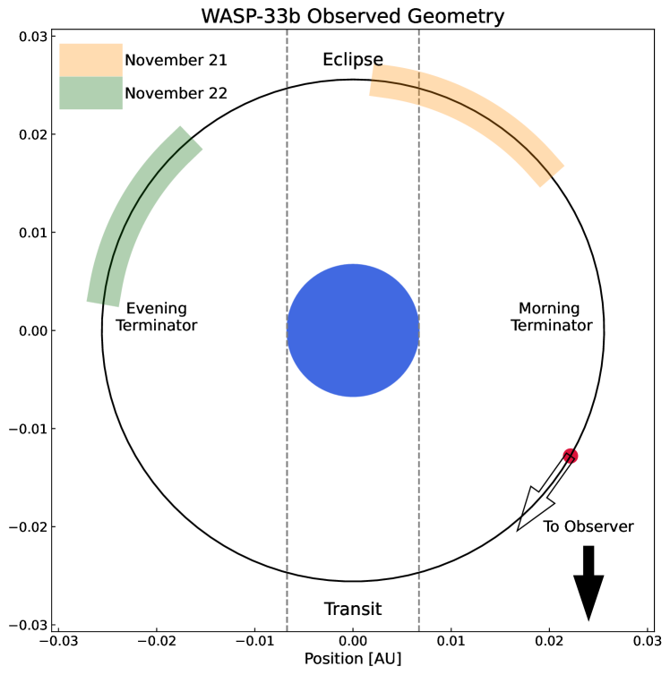
Our observations are summarized in Table 2. For all observations, we used an ABBA pattern nodding between KPIC science fibers 1 and 2. These fibers had the highest throughputs of the four science fibers in KPIC phase I (tested at the start of each night), and the nodding allows us to effectively subtract sky emission features and thermal emission from warm front-end optics on the Keck AO bench. We obtained 90-s exposures at each nod position, giving our observations a time resolution of approximately four minutes after read time/overheads and coadding frames. We chose a time resolution under five minutes based on simulations showing that the orbital motion of WASP-33b would begin to significantly broaden the final cross-correlation peak for longer timescales (known as Doppler smearing). Figure 1 presents a diagram of the system with the observed orbital phases shaded by observation date.
The 2021 November 21 observations began during secondary eclipse, providing a stellar spectrum with no planet contribution. Observations continued post-eclipse for just under three hours, covering roughly noon to mid-morning longitudes. Conditions were good, with throughput from the top of Earth’s atmosphere through detection peaking at consistently around 2.5%.
We attempted to obtain additional observations on 22 November covering late-evening to afternoon longitudes. However, high clouds caused significant extinction and poor AO performance, leading to top-of-atmosphere throughput consistently below 1%. We therefore omitted these observations from subsequent cross-correlation and retrieval analysis.
2.3 Data Reduction
We began by fitting the echellogram trace location and width for each fiber and order from observations of a bright calibrator star (typically the telluric standard for the wavelength calibrator, discussed below). Because the KPIC fiber-extraction unit (FEU) does not move relative to the spectrometer backend during science operations, this only needs to be done once per night. We then AB subtracted the science frames (taken in an ABBA sequence) to remove sky emission and thermal background. Spectral extraction was performed by summing over slices in the detector-Y direction (which is well aligned with the cross-dispersion direction) centered on the best-fit trace center with a width five times the standard deviation of the best-fit Gaussian.
Each fiber was individually wavelength-calibrated by comparing to a radial velocity standard following the procedure described in Section 3.2 of Wang et al. (2021). In brief, we observed a late-type giant star (HIP 95771 in the case of the WASP-33 observations) at the start of each night and fit the observed spectrum with a combined telluric spectrum generated using PSG (Villanueva et al., 2018) and stellar model from the PHOENIX library (Husser et al., 2013). Using a late-type star greatly increases the number of lines used for calibration compared with using only the sparse -band telluric absorption features, enabling a more robust calibration.
We next resampled all the extracted spectra from science fiber 1 onto the wavelength grid obtained for science fiber 2 using a cubic spline. While each fiber is stable in detector location and wavelength over a single night, manufacturing and alignment differences can lead to small variations between fibers in both fringing and LSF that we wish to average. We arrange the extracted spectra for each order into a times series, giving arrays each of shape . These arrays, along with the Julian date/time at the midpoint of each nod pair and the corresponding barycentric radial velocity to WASP-33 from Keck, are the inputs to our retrieval code. We omit the first three orders (blueward of 2.1 ) due to strong telluric contamination, and the following two orders due to wavelength calibration inaccuracies, leaving four NIRSPEC orders spanning m, with significant gaps. Additional post-processing performed as part of the retrieval is discussed in Section 3.1.1.
3 Atmospheric Retrieval
Our approach to atmospheric retrieval is similar to that of Line et al. (2021), with the most significant differences being our use of a negative injection of the proposed planet model (see Section 3.1.1) prior to the principal component analysis and the use of petitRADTRANS (Mollière et al., 2019, 2020) for radiative-transfer calculations. In brief, we use petitRADTRANS to generate simulated time-series spectra matched to our detrended observations, and calculate a log-likelihood following Brogi & Line (2019). We use this log-likelihood function to find best-fit orbital and atmospheric parameters using nested sampling (Skilling, 2004), specifically the dynesty (Speagle, 2020) implementation. We discuss the details of this procedure below.
3.1 Retrieval Procedure
3.1.1 Data Processing

At the end of the data reduction process, we can write each extracted spectrum as:
| (1) |
Where is the observed flux in each exposure, is the stellar flux and associated photon noise, including rotational broadening as well as limb and gravity darkening. is the planet flux and associated photon noise, which varies in time both due to the Doppler shift from the planet’s orbital motion and due to variations in the visible longitudinal range. describes telluric transmission, which varies in time as the airmass and precipitable water vapor change. encapsulates the spectrograph blaze function and flat-field effects and is stable over a given night. Finally, we describe the fringing with both a static term , arising from the NIRSPEC entrance window, and a time-varying term which is the result of the KPIC tracking camera dichroic and the pyramid wavefront sensor dichroic producing an etalon with a varying angle of incidence (Finnerty et al., 2022).
Because the projected radial velocity variation of WASP-33b over each observation sequence is substantially more than 3 the velocity resolution of NIRSPEC, taking a median of the time series should leave only the terms which do not vary significantly over time. However, frame-to-frame variations in coupling efficiency as a result of variable AO correction require that we first divide each spectrum by its median (see Figure 2, top panel) before taking the median over the time series. We can then write the time-series median spectrum as:
| (2) |
Where is the average stellar spectrum and represents the time-averaged telluric spectrum. We can then scale all spectra in the time series by the median and divide to obtain:
| (3) |
This is shown in the second panel of Figure 2. Both and vary around unity, so we can combine these terms and rewrite them as:
| (4) |
Using the above expression to rewrite equation 3 and expanding gives:
| (5) |
At this point, a number of approaches have been used to remove the time-varying systematic noise/telluric residual term (note that the cross term can generally be taken to be smaller than the others). One approach, used in e.g. Brogi & Line (2019); Pelletier et al. (2021), is to fit and divide a low-order polynomial to the time series of each spectral channel. This is effective when the temporal variation is slow, such as airmass-induced variations, and may be followed by additional processing such as PCA. For KPIC data, the time-varying fringe cannot be corrected with this approach, and we therefore do not use it.
An additional or alternative technique used in e.g., Pelletier et al. (2021); Line et al. (2021), is to perform principal component analysis (PCA) on the time series. PCA is a dimensionality reduction technique which projects the observed spectra onto a basis which maximizes the time-series variation in each successive component. This allows most of the variation in the time series to be encapsulated in the first few principal components, which can then be “zeroed-out” via a projection matrix in order to eliminate the variation. While this effectively eliminates most of the time-varying tellurics and fringing, it also removes/distorts some of the planet signal we are attempting to retrieve. This can be minimized by using the smallest number of principal components (PCs) needed to eliminate tellurics/fringing, as the planet signal is generally much lower amplitude and therefore should be more present in higher PCs.
The distortion of the spectrum caused by PCA can then be estimated by using the calculated PCs to apply a similar “stretch” to the data (Line et al., 2021). Specifically, we can write the observed flux, post-PCA and median division, as:
| (6) |
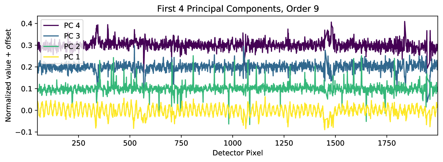
Where we have subtracted the bias term from Equation 5. represents the dropped principal components, which we use to “stretch” the model in our log-likelihood calculations and reproduce the term. Note that this assumes does not contain any contribution from , which is generally not valid, although the contribution may be negligible in some cases. These processing steps may inadvertently impact the strength of the planet features relative to the continuum. We therefore include a multiplicative scaling to the planet model () as a free parameter in our retrievals, which we expect to be of order unity. The third panel of Figure 2 shows the post-PCA time series for one order, with the time-varying fringing effectively removed. We show an example of the dropped principal components in Figure 3, which appear to be dominated by fringing and airmass variation.
Occasionally the post-PCA data show a temporally fixed fringing pattern at much lower amplitude than the original fringe. While Figure 2 indicates this is not substantially impacting these observations, we include a second median division after PCA in order to eliminate any residual fringing, though doing so does not appear to impact the results of our retrievals. The fourth panel of Figure 2 shows the time series after this final division and an additional masking of values differing from the median by (approximately 6 times the median absolute deviation)
3.1.2 Negative Injection and Number of PCs
Our initial tests found that removing 4 PCs enabled a detection of WASP-33b at a velocity similar to previous results from the literature (e.g. Nugroho et al., 2021; van Sluijs et al., 2022). However, PCA will remove or distort the underlying planet signal, which must be mitigated in order to run retrievals. We adopt a negative-injection approach, where we subtract the proposed planet/star time series from the observed prior to performing the PCA. In the case where the planet model accurately reproduces the data, this eliminates the PCA self-subtraction issue, while potentially exaggerating it for poorly-matched models. This approach is sensitive to the exact match between the observations and the template, requiring PCA to be performed as part of each logL evaluation. While this significantly increases the computational cost of each log-likelihood call, it should reduce the sensitivity of the retrieval to the precise number of omitted principal components.

Using PCA requires a decision as to the number of principal components to omit. Removing too few principal components can lead to significant contamination from fringing or tellurics, while removing too many can distort or even eliminate the planet signal. We believe that our negative-injection approach should substantially reduce the sensitivity of the planet detection to the number of omitted PCs, provided the planet is injected at approximately the correct strength relative to the continuum.
To test the impact of varying the number of omitted PCs, we computed the stellar-frame cross-correlation function of the maximum-likelihood retrieved planet spectrum with each frame in the 21 November data for varying numbers of omitted PCs. This is shown in Figure 4, where the CCF has been divided by the variance for in order to estimate the signal-to-noise ratio. We then shift to the planet rest frame and sum in order to estimate a 1D CCF. Without PCA, the 2D cross-correlation space is clearly dominated by the time-varying fringe, and the planet signal is barely detectable even in the stacked CCF. Between 2 and 10 omitted principal components, the planet signal is clear even in the 2D CCF, and the number of PCs dropped does not appear to significantly change the CCF.
The apparent independence of the planet detection on the number of PCs makes the choice of how many PCs to omit somewhat arbitrary. We opted to omit 4 PCs based on examination of the components in Figure 3, which show substantial contributions from fringing and tellurics in these components. While Figure 4 suggests we could safely drop additional components, we are concerned that model mismatch may still result in self-subtraction when many PCs are dropped, despite the negative injection. Omitting 4 components is a qualitative balance between removing known contaminants while avoiding self-subtraction issues and is consistent with other high-resolution retrievals (e.g Line et al., 2021). For consistency and to avoid possible overfitting, we omit the same number of components for and all orders. In the future, it would be preferable to develop and use a quantitative set of criteria for the number of PCs to remove. Alternatively, improved forward modeling of the KPIC fringing could reduce or eliminate the need for PCA.
3.1.3 Template Spectra and Opacities
Calculating a log-likelihood requires comparing the detrended time series obtained from the steps described in the previous subsection to an analogous simulated data set with known orbital and planetary parameters. This requires models of both stellar and planetary spectra in order to calculate the equivalent to the term obtained above.
For the stellar template, we use a PHOENIX model (Husser et al., 2013) with , , and , chosen to be similar to the stellar parameters in Table 1. We then simulate the observed stellar disk as a 6060 array of these 1D spectra, Doppler shift by the expected at the location of each grid point on the stellar disk, and apply limb darkening coefficients from Sing (2010). We neglect the impacts of both gravity darkening and the Scuti pulsations of WASP-33. Each of these may lead to an achromatic systematic offset between our simulated and the true stellar spectrum, which the scaling parameter in the retrieval should account for. We note that Cauley et al. (2021) reported the pulsation of WASP-33 leads to time-varying velocity shifts in the cross-correlation function for high resolution optical data. We do not expect this phenomenon to impact -band observations, as we do not anticipate H2O or CO features in the A-type stellar spectrum.
For the planet templates, we use petitRADTRANS (Mollière et al., 2019, 2020) to perform the radiative-transfer calculation with 80 log-uniform spaced pressure slabs from bar to bar and a spectral resolution of over the – range covered by our observations. We use molecular opacities for CO, H2O, and OH generated using ExoCross (Yurchenko et al., 2018) from the HITEMP linelists (HITEMP 2010 for H2O, HITEMP 2019 for CO, HITEMP 2020 for OH; Rothman et al., 2010; Gordon et al., 2022). We use the Li et al. (2015) partition function for CO, the Polyansky et al. (2018) partition function for H2O, and the Yousefi et al. (2018) partition function for OH. For SiO, we use the ExoMol-recommended linelists and partition functions from Yurchenko et al. (2021). Opacities are generated on pressure-temperature grids ranging from – bar in pressure and from 80–6000 K in temperature, which petitRADTRANS interpolates to the desired pressure/temperature values for each layer. We allow molecular abundances for each species to vary freely during the retrieval but hold abundances constant at all pressures.
3.1.4 Pressure-Temperature Profile
To describe the atmospheric temperature at each pressure layer, we use the pressure-temperature (PT) profile parameterization from Madhusudhan & Seager (2009). This 6-parameter model divides the atmosphere into three zones — two upper zones with exponential behavior and an isothermal lower atmosphere. Using two upper zones allows this model to fit both inverted and non-inverted PT profiles, and the isothermal lower atmosphere is expected for hot Jupiters due to high optical depths (Madhusudhan & Seager, 2009). Based on previous results from WASP-33b (Nugroho et al., 2021; van Sluijs et al., 2022; Yan et al., 2022) we require a thermal inversion for the dayside PT profile. This requirement speeds convergence and avoids issues with fitting inverted sidelobes of the cross-correlation function. We also enforce throughout the atmosphere in order to avoid hitting the limits of our opacity tables.
3.1.5 H-
The temperature and irradiation of WASP-33b suggest a significant fraction of upper atmospheric H2 may be dissociated, and H- may be a significant source of continuum opacity. We experimented with several ways of incorporating H-. Our first approach used the poor_mans_nonequ_chemistry calculator from petitRADTRANS (Mollière et al., 2017, 2020) to estimate the chemical equilibrium H2, He, H, H-, and e- fractions in the atmosphere for the proposed PT profile, which petitRADTRANS then uses to calculate H- opacity. While this accounts for the strongly-varying vertical abundance of H-, this is inconsistent with our free-retrieval approach used for other species. We next attempted to include H- and e- as species in the retrieval, but both were effectively unconstrained over a prior based on the typical equilibrium chemistry values.
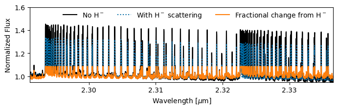
Finally, after comparing model planet spectra with and without H- (see Figure 5), we opted not to include H- opacity in our retrievals. We find that on the scale of a single NIRSPEC order, H- is effectively achromatic, resulting in a consistent reduction in line strengths (see Figure 5, orange line) relative to the continuum. As we do not preserve the continuum level through the detrending process, the overall scaling parameter is already effectively scaling the line strengths relative to the continuum, making the additional inclusion of H- opacity redundant. The CO and H2O abundances retrieved without H- opacity are statistically consistent with the retrievals including H- based on equilibrium abundances.
Neglecting H- should result in a smaller value for the scaling parameter, as the lines will be weaker relative to the continuum than we assume. This achromatic behavior may not hold over wider bandpasses, in which case H- should be included in the retrieval model.
3.1.6 Model Processing
Using the planet spectra calculated by petitRADTRANS, we next calculate a model time series. We first scale the planet flux by the planet/star area ratio and then Doppler shift the planet to the proposed velocity for each exposure. We subsequently divide the planet model by the stellar model, Doppler shift by the systemic velocity, and interpolate onto the observed wavelength grid. We then convolve the model spectrum with a 1.7 pixel Gaussian representing the NIRSPEC instrument profile and divide by the time-series median. The optimum kernel was determined by maximizing the log-likelihood at the planet peak identified in a diagram with a fixed planet template and is slightly larger than expected based on the instrument resolution, most likely as a result of the motion of WASP-33b along its orbit within a single set of exposures(known as Doppler smearing). Finally, we apply the PCA “stretch” to the model and perform a second median division in order to match the treatment of the observations. At this point the model spectra should be exactly analogous to the data, and we calculate the log-likelihood as described in Brogi & Line (2019).
3.1.7 Parameter Selection
| Name | Symbol | Prior |
|---|---|---|
| Upper-atmosphere scaling | Uniform(0,1) | |
| Lower-atmosphere scaling | Uniform(0,1) | |
| Top-of-atmosphere temperature [K] | T | Uniform(2000, 6000) |
| Reference pressure [bar] | log P1 | Uniform(-6, 0) |
| Mid-atmosphere fraction | Uniform(0,1) | |
| Lower-atmosphere fraction | Uniform(0,1) | |
| offset [ ] | Uniform(-40, 40) | |
| offset [ ] | Uniform(-30, 30) | |
| log H2O mass-mixing ratio | log H2O | Uniform(-6, -1) |
| log CO mass-mixing ratio | log CO | Uniform(-6, -0.1) |
| log OH mass-mixing ratio | log OH | Uniform(-6, -1) |
| log SiO mass-mixing ratio | log SiO | Uniform(-6, -1) |
| log | Uniform(-2.5, -0.5) | |
| Total H mass-fraction | log allH | Uniform(-0.2, -0.05) |
| HI fraction | Uniform(0, 1) | |
| Scale factor | scale | Uniform(0, 2) |
, in order to avoid going beyond the bounds of our opacity grids.
Our retrieval model consists of 16 free parameters. We list these parameters and priors in Table 3, and provide a brief description and motivation here. For the PT profile, we adopt the six-parameter model from Madhusudhan & Seager (2009), setting . This takes a top-of-atmosphere temperature, two coefficients to scale the argument of the exponential functions, and three reference pressures for the transition between the different exponentials and the isothermal lower atmosphere. We implement this as a single physical pressure, and two fractional breakpoints (in log space) between that pressure and the top/bottom of the atmosphere respectively. This allows inequality constraints to be more easily placed on the different pressures in order to enforce the presence/absence of a thermal inversion. We choose priors for the temperature based on previous literature values (Nugroho et al., 2021; van Sluijs et al., 2022), while we allow the scaling and pressure parameters to vary over a broad range. We require a thermal inversion based on the initial qualitative cross-correlation analysis discussed in Section 4 and previous literature (Nugroho et al., 2021; Yan et al., 2022; van Sluijs et al., 2022).
We also fit two parameters for the orbital properties of WASP-33b. While the planet radial velocity semi-amplitude () and systemic velocity () are well-constrained by previous literature, the 3D atmospheric structure may introduce phase-dependent velocity shifts due to winds or outflows (Beltz et al., 2022). We choose priors based on the approximate extent of the planet peaks obtained from cross-correlation with an assumed template (see Figure 6) and to cover the range of values reported in van Sluijs et al. (2022).
We fit for seven abundances – H2O, CO, OH, SiO, H2, the 13CO/12CO ratio, and the H2 dissociation fraction. H2O and CO are expected to dominate the -band spectrum for UHJs and are expected to be the dominant forms of C, O, and overall metals in the atmosphere of WASP-33b. We also include , as we expect it to be detectable in an atmosphere with a high overall CO abundance (Mollière & Snellen, 2019). While simulations suggested that the limited wavelength coverage of our observations may be insufficient to make an independent detection of OH, we include it for completeness based on the previous dayside detection reported by Nugroho et al. (2021), which used prominent OH features in the -band. Brogi et al. (2023) also detected OH in the atmosphere of the UHJ WASP-18b with -band observations. We also fit for SiO, as the petitRADTRANS equilibrium chemistry models suggest that it may be a significant oxygen reservoir in the high-C/O, high-metallicity regime, and (Cont et al., 2021) previously reported a detection of atomic Si in the dayside upper atmosphere of WASP-33b. The final abundance parameters are the total (molecular and atomic) hydrogen mass fraction and the H2 dissociation fraction. The remainder of the atmosphere is assumed to be entirely He.
Finally, we fit an additional multiplicative scaling parameter applied to the planet model. This accounts for a number of possible biases in our retrieval setup, while also serving as a check for their severity. Ideally, we should retrieve a scaling parameter of 1. However, we neglected both Scuti pulsations and gravity darkening of the host star, which may introduce systematic differences in the relative flux of the planet. We also ignore H- opacity in the planet atmosphere, which could produce achromatic changes in the line strengths. The scale factor allows us to correct for these omissions, while also checking the size of these effects.
3.1.8 Nested Sampling
We compare our forward-models described above to the processed observations using the log-likelihood function from Brogi & Line (2019). Specifically:
| (7) |
Where is the number of valid points in each observed spectrum, is the cleaned data, and is the proposed spectrum, which already includes the scaling parameter. This is calculated for each order and each science frame taken out-of-eclipse, then summed to produce a total log-likelihood for the observation sequence.
This log-likelihood calculation enables us to use the full range of Bayesian fitting tools. As in Line et al. (2021), we opt for a nested-sampling approach (Skilling, 2004), in our case the dynesty implementation (Speagle, 2020). Nested sampling is suitable for high-dimensional problems with computationally expensive likelihood functions and potentially complicated posteriors, making it ideal for atmospheric retrievals. It is also easily parallelizable, allowing us to take advantage of cluster computing resources. Our retrievals using 16 CPU slots typically take 2–4 days to reach , which is sufficient to obtain good estimates of the posteriors.
3.2 Validation Simulations
| Symbol | Input | Retrieved |
|---|---|---|
| 0.48 | ||
| 0.10 | ||
| T | 3420 | |
| log P1 | -2.6 | |
| 0.29 | ||
| 0.42 | ||
| [ ] | 0 | |
| [ ] | 0 | |
| log H2O | -4.3 | |
| log CO | -1.5 | |
| log OH | -2.5 | |
| log SiO | -3.7 | |
| log | -1.8 | |
| log allH | -0.13 | |
| log | 0.42 | |
| scale | 1.0 | |
| 110 |
As our retrieval framework by necessity includes a forward-modeling capability, we can easily test our retrievals on a simulated system with known inputs. This provides a check on systematic biases in the retrieval and ensures that the reported uncertainties are reasonably accurate. These checks also allow us to determine if any parameters are inherently poorly constrained by the available data. All simulated data sets used the same orbital phase sampling as the observations (2021 November 21).
As our forward modeling does not include fringing or airmass variation, we do not include the PCA step in the test retrievals. The planet spectrum is the only time-varying component in the simulated spectrum. Even with our negative-injection approach, the planet spectrum is distorted by the PCA in the absence of stronger fringe/airmass-induced variations. This limits our ability to identify biases introduced from the PCA and may result in a mild overestimation of the retrieved errors in the simulations, as the negative-injection PCA approach is expected to increase preference for the true planet model. Ongoing developments in forward modeling of the KPIC fringing should reduce future reliance on PCA for defringing.
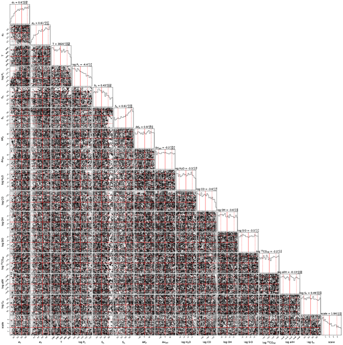
Our first test case was a star-only (no planet) simulated data set. This provides a non-detection baseline for comparison. Figure 10 shows the full corner plot (Foreman-Mackey, 2016) in Appendix A. Despite using the same stopping criteria as other retrievals, the star-only simulation shows much flatter and noisier posteriors and reached the stopping criteria in far fewer iterations. Additionally, the scale parameter shows a weak preference towards smaller values, suggesting a preference for the absence of the planet, as expected. The retrieved pressure-temperature profile is nearly isothermal, and the maximum-likelihood planet spectrum is nearly flat, as the fitting minimizes the strength of the planet features.
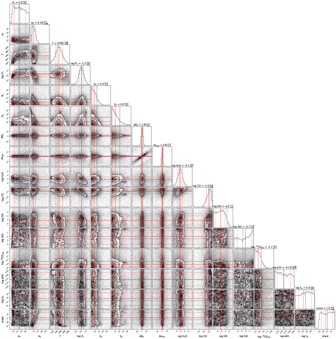
Our second test case was based on the retrieved parameters for WASP-33b listed in the “Input” column of Table 4. The signal-to-noise ratio of the simulations was chosen to be similar to that of the observations. This provides both a general check for systematics or unconstrained parameters in our retrieval framework as well as a specific injection/recovery test for the retrieved dayside atmosphere. Retrieved values and uncertainties are listed in the “Retrieved” column of Table 4, and the full corner plot is presented in Figure 11.
All parameters except the OH mass fraction are retrieved to within 1 of the input values, with error bars similar to those retrieved from the observations. The PT profile retrieved from the simulations is slightly hotter than the input profile but is generally within the 1 bound and does not impact the retrieved abundances. The SiO mass fraction, H mass fraction, and H dissociation fraction are all poorly-constrained in both the observations and the simulated retrieval, suggesting our observations have limited sensitivity to these parameters.
While the OH posterior shows a peak in the observations, this is not the case in the simulated retrieval. The 13CO isotopologue ratio and the scale factor are also better-constrained in the observations than the simulations, though not to the same degree as the OH abundance. While this may be a result of the negative-injection PCA approach used for the observations improving sensitivity to relatively small changes in the spectrum, the poor sensitivity in simulated retrievals suggests both apparent constraints may be artifacts.
We also ran retrievals using emcee (Foreman-Mackey et al., 2013). This provides a check that any biases are not due to the particulars of our nested sampling approach, such as the stopping criteria or the number of live points. The resulting median values and uncertainties from emcee were consistent with the nested sampling results. This suggests that systematics are more likely to be related to limitations in the radiative transfer calculation, log-likelihood function, or inherent limitations in the data, rather than the statistical framework used.
4 Results
We present qualitative results from cross-correlation analysis in Section 4.1. Quantitative results from our retrieval framework are presented in Section 4.2.
| Name | Symbol | Retrieved |
|---|---|---|
| Upper-atmosphere scaling | ||
| Lower-atmosphere scaling | ||
| Top-of-atmosphere temperature [K] | T | |
| Reference pressure [bar] | log P1 | |
| Mid-atmosphere fraction | ||
| Lower-atmosphere fraction | ||
| offset [ ] | ||
| offset [ ] | ||
| log H2O mass-mixing ratio | log H2O | |
| log CO mass-mixing ratio | log CO | |
| log OH mass-mixing ratio | log OH | |
| log SiO mass-mixing ratio | log SiO | |
| log | log | |
| Total H mass fraction | log allH | |
| HI fraction | ||
| Scale factor | scale | |
| Derived Parameters | ||
| C/O ratio | C/O | |
| log C/HVMR | log C/H | |
| log O/HVMR | log O/H |
4.1 Cross-Correlation Analysis
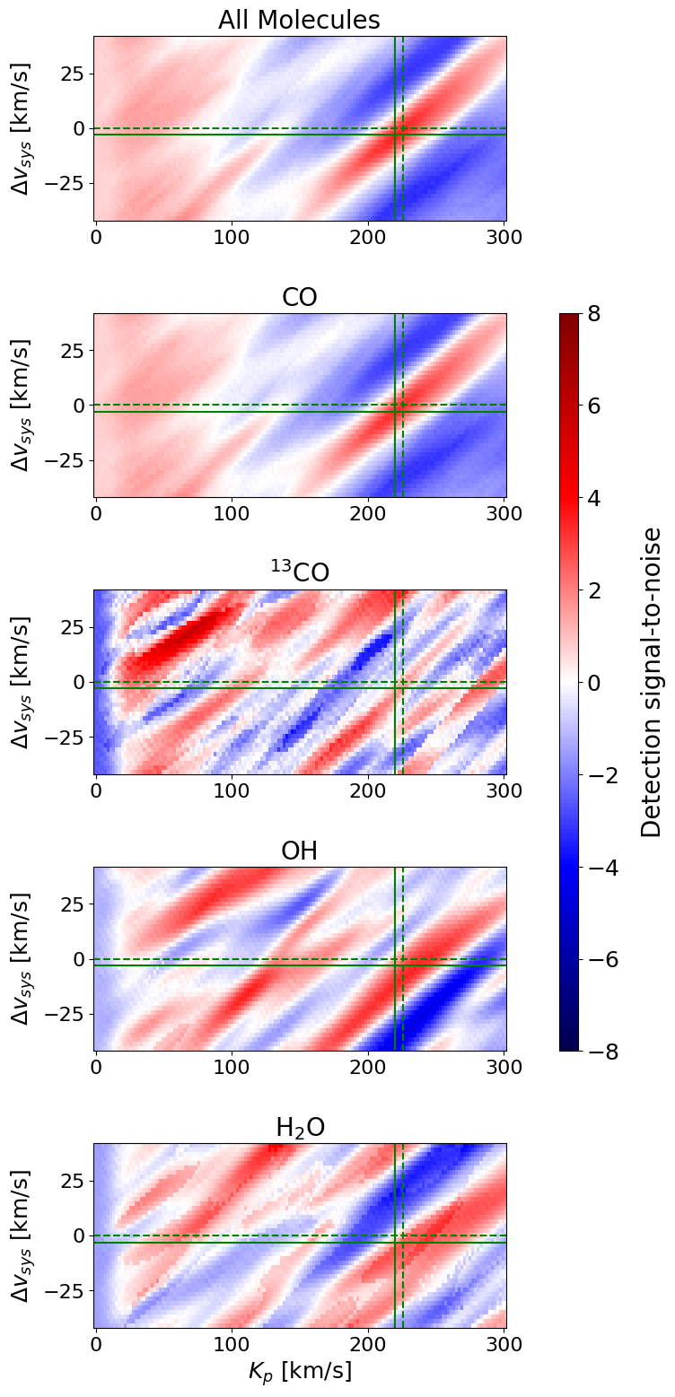
We use the best-fit retrieval parameters to compute diagrams, both for the overall model and for each individual species. These are plotted in Figure 6, with the retrieved and values indicated in dashed green. This is the approach that previous high-resolution studies have used to make molecular detections (e.g. Brogi et al., 2012; Buzard et al., 2020, and many others). We note that attempts to quantify strengths for this type of detection have been fraught (e.g. Buzard et al., 2020; Finnerty et al., 2021; Buzard et al., 2021), but these plots can still provide useful qualitative insight.
Specifically, quantitative estimates of the detection strength from plots typically assume values far from the planet peak are normally-distributed and use the standard deviation far from the planet as an estimate of the noise. In the case of Figure 6, this is complicated by the clear presence of systematic variations as a function of due to the detrending suppressing the planet at small . We therefore estimate the noise in Figure 6 by first masking to exclude the region where the PCA is having a significant impact, then additionally masking values above/below the 10th/90th percentile to remove the planet feature. We then calculate the standard deviation and use this to make the detection strength map. These thresholds are arbitrary, and the remaining points after masking still do not appear to be normally distributed. We emphasize that Figure 6 is intended for a qualitative assessment of the detection of different species. For a quantitative assessment, Figure 4 is better for estimating the strength of the overall detection, and Table 6 presents Bayes factors for the detection of each molecules.
The strong dependence of the detrending signal on allows it to be removed by subtracting each column of Figure 6 by its median. This results in a detection strength of 0 at , as expected when the planet is totally removed by detrending. For the all molecule case, the planet is detected at an SNR12, which is more consistent with expectations based on Figure 4 than the scale of Figure 6. However, this removal of the detrending systematics is not statistically rigorous. We emphasize that Figure 4 offers the most robust estimate of the overall detection strength.
The planet is clearly detected in the diagram plotted in the top panel of Figure 6. In the 2D plots of cross-correlation versus time in Figure 4, planet velocity track is clearly visible, and the retrieved velocities are in good agreement with the nominal values. Additional validation of the detection is provided by the disappearance of the planet feature during secondary eclipse in Figure 4.
The cross-correlation detection is dominated by based on comparing the first and second panels of Figure 6. OH also produces a strong signal at the expected location in the space (fourth panel of Figure 6), while the H2O template produces a somewhat weaker signal (fifth panel of Figure 6). The template has a weak feature coincident with the expected planet velocity, but this feature does not dominate and we do not consider this to be an independent detection of . The SiO template does not produce any features in the space and is not shown.
4.2 Retrieval Results
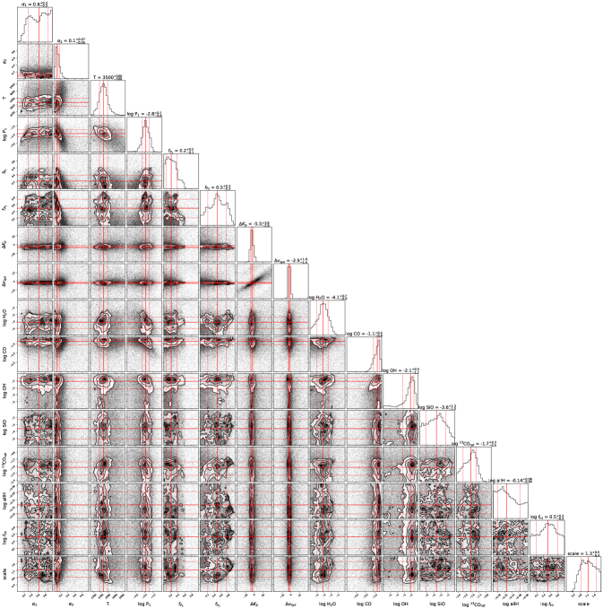
Retrieved atmospheric parameters are listed in Table 5. The full corner plot (Foreman-Mackey, 2016) for the retrieval is presented in Figure 12. The retrieved dayside PT profile, emission contribution function, and median spectrum are plotted in Figure 7.
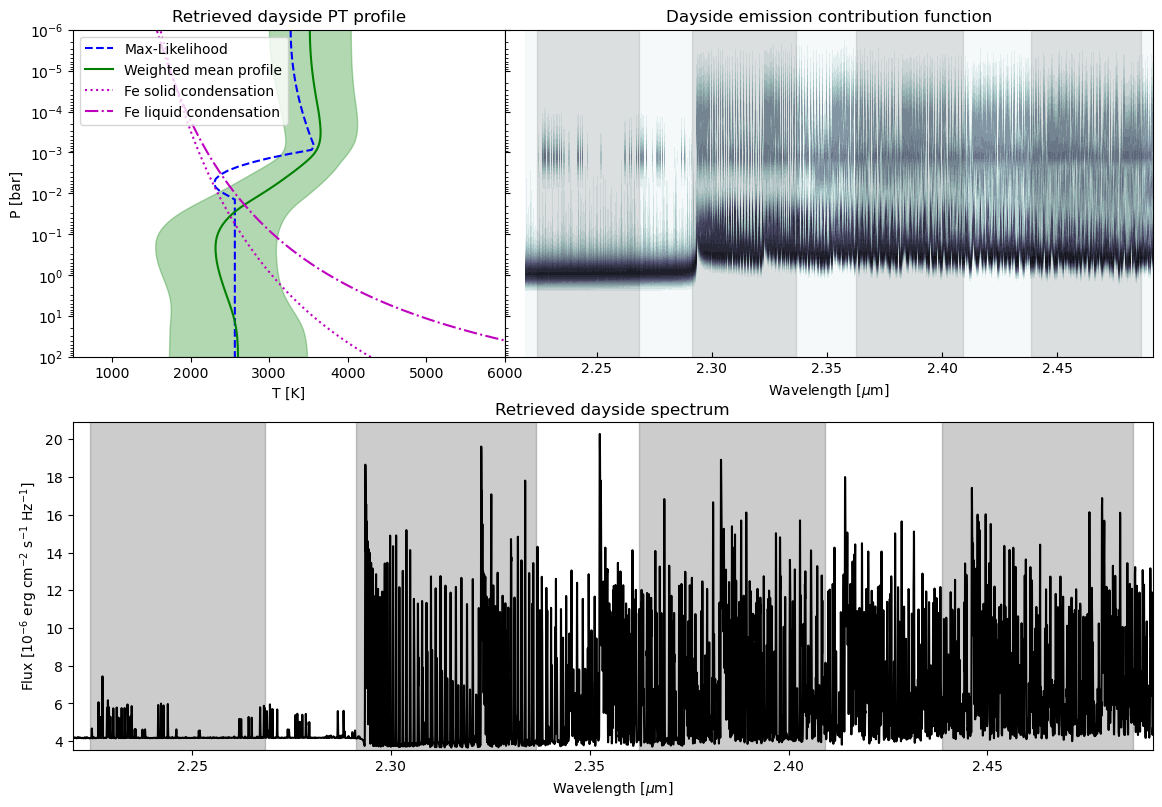
The dayside atmosphere shows a clear inversion beginning at approximately 0.1 bar, consistent with previous results (e.g. Nugroho et al., 2021; van Sluijs et al., 2022). The -band emission contribution function (Figure 7, top right panel) indicates that the bulk of the observed emission arises near this pressure, though CO continues to contribute to the line cores from altitudes up to bar. Pressures greater than bar do not contribute to the observed emission, and the retrieved PT profile is therefore unlikely to be accurate at these pressures. We note that the high-resolution spectroscopy is sensitive to the line strength relative to the continuum, which is determined by the shape and contrast of the PT profile, the atmospheric metallicity, the scaling parameter, and possible impacts from H-. This can allow “cold” PT profiles to produce similar output spectra to those of “hotter” PT profiles. While temperature will also change the relative strengths of different lines, this is a comparatively small effect over a limited bandpass. We therefore caution against relying on the exact temperatures of the retrieved PT profiles.
We obtain log mass fractions of for H2O, for CO, and for OH. This indicates that H2O is almost entirely dissociated on the dayside of WASP-33b, consistent with previous findings from Nugroho et al. (2021). SiO is effectively unconstrained due to its relatively low -band opacity, but peaks at a log mass fraction of , which would be consistent with the neutral Si detection reported in Cont et al. (2022a). We also obtain a weak constraint on the 13CO/12CO ratio, peaking around but with a significant tail giving a median value of . The abundance parameters show a strong positive covariance, which enables better constraints on the C/O ratio than would be expected from the marginalized uncertainties.
Finally, we note that while the scaling parameter peaks near unity, there is a long tail towards higher values. The scaling parameter controls the strength of lines relative to the host star continuum, which can also be influenced by changes in the PT profile. Figure 12 shows weak degeneracies between the PT profile parameters and the scaling parameter, with larger values of the scaling parameter corresponding to PT profiles which produce weaker lines. This suggests the tail of the scaling parameter is a result of under-constraining the PT profile.
There are a number of systematics or physical effects that could also change the value of the scaling parameter. Our test retrievals suggest this may be a result of our data processing (see Figure 11). Physical factors include underestimates of the planet radius or temperature, H- opacity, thermal expansion of the dayside atmosphere, extended emission from an outflow, or stellar pulsations. The retrieved posterior peaks at a scale factor , suggesting that these effects are either relatively minor or largely cancel.
5 Discussion
We present Bayes factors for the detection of each molecule compared with a flat planet model in Table 6 and discuss the detection significance for each molecule in Section 5.1. We discuss the retrieved wind speeds and thermal structure in Section 5.2. The C/O ratio and metallicity of WASP-33b are discussed in Section 5.3, including a comparison to equilibrium chemistry models. We discuss the weak constraint retrieved for the CO isotopologue ratio in Section 5.4 and finally discuss the implications of our results for the formation history of WASP-33b in Section 5.5.
5.1 Detection Confidence
| Model | Bayes Factor |
|---|---|
| All molecules | 111 |
| CO only | 102 |
| 13CO only | 9.8 |
| H2O only | 6.9 |
| OH only | 5.6 |
To assess the strength of our detections, we compute the Bayes factor comparing a flat/no planet model and the best-fit models for all molecules together and for each molecule independently. These values are presented in Table 6. The best-fit planet model is strongly preferred () , with CO dominating the detection. The evidence for H2O and OH is substantial but weaker than CO, consistent with expectations based on the weaker features in the space in Figure 6.
5.2 Winds and Thermal Structure
Consistent with both previous results (Nugroho et al., 2021; van Sluijs et al., 2022) and global circulation models of UHJs (Wardenier et al., 2021; Komacek et al., 2022; Beltz et al., 2022), our retrievals confirm our assumption of a thermal inversion on the dayside. We find that constant offsets in the PT profile appear to have a limited impact on the final spectrum, suggesting our observations are not particularly sensitive to absolute temperature, with the curvature of the PT profile having a much more substantial impact. The inclusion of the scaling parameter may compound this, as it provides an alternative way to change line depths in the planet model. Figure 7 shows that our -band observations are most sensitive to a relatively narrow range of pressures and therefore have limited ability to constrain the overall PT profile. Additional observations at other bands may improve the vertical constraints.
The velocity parameters prefer a slight blueshift compared to the nominal values in Table 1. While this could be a result of morning-to-evening winds, the shift is only 1-2 and is well within the model-dependent variations in velocity parameters reported in van Sluijs et al. (2022). Additional observations providing continuous coverage of a larger phase range would provide better constraints on dayside winds.
We adopted the systemic velocity from Gontcharov (2006). More recent observations have found in the range of -3 (Collier Cameron et al., 2010) to 0 (Nugroho et al., 2021). van Sluijs et al. (2022) found systemic velocities from -15 to +6 , depending on the orbital phase of the observations and the type of model used for cross-correlation. A more positive systemic velocity would imply larger blueshifts in the retrieved planet parameters relative to the expected Keplerian motion in the host star reference frame.
5.3 C/O ratio and Metallicity


The retrieved abundances yield a gas-phase . The derived posteriors for C/H, O/H, and C/O are shown in Figure 8. However, these retrievals are missing several potential oxygen reservoirs in ultra-hot Jupiter atmospheres, whose presence in significant quantities would lower the atmospheric C/O ratio. Metal oxides including TiO (Cont et al., 2021; Serindag et al., 2021) and AlO (von Essen et al., 2019) have previously been detected in WASP-33b, neutral atomic oxygen has been detected in the similar UHJ KELT-9b (Borsa et al., 2021), and Si has been detected in low-pressure ( mbar) optical observations of WASP-33b (Cont et al., 2022a), suggesting the possible presence of SiO deeper in the atmosphere. Our limited wavelength coverage precludes detection of any of these species, though a significant reduction in C/O as a result would require either significant neutral oxygen or an atmosphere substantially enriched in refractory elements compared with volatiles.
The atmospheric metallicity of WASP-33b is more difficult to infer from these observations than the C/O ratio. The retrieved abundances suggest a moderately metal-enriched atmosphere, but the lack of continuum information in high-resolution observations leads to strong correlations between species abundances, making absolute abundance estimates difficult. Previously, Cont et al. (2022a) found a solar-metallicity model best explained the observed Si signal, though they used a widely-spaced model grid. In subsequent analysis Cont et al. (2022b) estimated a metallicity of +1.5 dex based on retrievals of several atomic species from optical data, including Ti, Fe, and V, consistent with the retrieved metallicity from the KPIC observations.
In order to better understand the range of possible C/O ratios and metallicities, we compare our retrieved abundances with grids of equilibrium chemistry models from the poor_mans_nonequ_chem package of petitRADTRANS (Mollière et al., 2017, 2019). These comparisons are plotted in Figure 9. In our parameterization scheme, the CO abundance is determined primarily by the atmospheric metallicity, while the H2O/OH abundance is significantly impacted by the C/O ratio. As the equilibrium grid does not include OH, we assume the equilibrium H2O abundance as the prediction for the dayside OH abundance.
Figure 9 shows the retrieved abundances are most consistent with equilibrium models having and C/O = 0.8. These values are consistent with Thorngren & Fortney (2019) modeled upper limits on metallicity for a planet the mass of WASP-33b as well as the retrieved metallicity from Cont et al. (2022b) based on optical observations. However, varying the in the chemical model suggests that our metallicity uncertainty is approximately 1 dex, and we therefore cannot confidently exclude stellar or even sub-stellar atmospheric metallicities for WASP-33b. C/O appears to be better constrained, with a margin consistent with the posterior shown in Figure 8. Note that the strong covariance between species abundances suggests that this C/O ratio will hold even if the metallicity varies significantly (see Figure 8).
The chemical equilibrium models suggest significant SiO abundances at the pressures probed by our observations. At lower pressures, the SiO abundance drops due to thermal dissociation, consistent with the optical detection of Si by Cont et al. (2022a). While our -band observations are not sensitive to SiO, -band observations of the SiO bands from 4–4.2 m could measure the SiO abundance. Assuming SiO is the dominant undetected oxygen reservoir at bar pressures, this would significantly improve estimates of the overall oxygen abundance.
5.4 CO Isotopologue Ratio
The posterior peaks at , with a tail towards lower values bringing the median to . While the posterior is somewhat poorly-constrained, the fact that we see even a weak preference is an argument in favor of high abundances. In simulated observations, mass-mixing ratios as high as do not always lead to a preference in the isotopologue ratio posterior. The peak of this weak preference is consistent with estimated CO isotopologue ratios from protoplanetary disks (Woods & Willacy, 2009) and is consistent with the value measured for WASP-77Ab in Line et al. (2021). Constraints on isotopologue ratios as well as abundances may provide a complementary path to probing formation history and physical conditions in exoplanetary atmospheres (Mollière & Snellen, 2019; Zhang et al., 2021).
5.5 Implications for Planet Formation
The high-C/O, potentially high-metallicity atmosphere suggested by our retrievals is consistent with the Pelletier et al. (2021) observations of the hot Jupiter Boo b. These observations conflict with predictions from pebble accretion models that atmospheric metallicity and C/O ratios should be inversely correlated, as secondary pebble accretion is expected to be dominated by oxygen-rich grains (Espinoza et al., 2017; Madhusudhan et al., 2017; Cridland et al., 2019; Khorshid et al., 2021). High C/O, high-metallicity atmospheres require formation and/or substantial accretion in an environment that is enriched in both carbon and solids. Such conditions are consistent with models that incorporate pebble drift (Booth et al., 2017), formation near CO or CO2 snow lines (Öberg et al., 2011), or with pollution by C-rich grains interior to the H2O snow line (Chachan et al., 2023).
As discussed in Section 5.3, one possible explanation for this discrepancy is that our -band high-resolution retrievals are simply missing a significant source of oxygen. Figure 9 suggests relatively high SiO abundances for WASP-33b, which we cannot measure with our -band observations. However, comparison with the equilibrium chemistry models suggests including SiO would not substantially decrease the C/O ratio under equilibrium conditions without substantial enrichment of Si relative to other metals (see Figure 9, third panel) Alternatively, additional oxygen could be present in the atomic form, as (Borsa et al., 2021) reported from transit observations of KELT-9b. In the future, Keck/HISPEC will offer simultaneous yJHK coverage at R (Mawet et al., 2019) with substantially improved throughput compared with KPIC, enabling characterization of a broader range of chemical species and reducing the likelihood of missing significant oxygen or carbon reservoirs.
Missing oxygen could also be the result of errors in linelists or molecular opacity calculations rather than chemistry. A poorly-matched H2O or OH opacity in the retrieval setup could lead to a bias towards lower abundances. However, both this work and Pelletier et al. (2021) retrieved high-C/O atmospheres using different H2O opacity tables and linelists, indicating that such an error would have to be systematic across multiple independent calculations, while simultaneously not significantly impacting the same calculations for CO. This suggests that the problem would have to be related to a common assumption specific to the H2O high-temperature linelists. Computing high-resolution, high-temperature H2O opacities for the -band alone required nearly one year of CPU time using exocross (Yurchenko et al., 2018), limiting our ability to compute and compare multiple opacity tables.
Alternatively, superstellar metallicity and C/O may arise either from accretion near evaporation fronts close to snow lines (Öberg et al., 2011) or from carbon-rich grain accretion between the carbon soot line and the H2O snow line (Chachan et al., 2023). Pebble accretion studies have found grain accretion within the snow line should boost oxygen abundances rather than carbon (e.g. Madhusudhan et al., 2017; Espinoza et al., 2017; Cridland et al., 2019), but models incorporating pebble drift can produce giant planet atmospheres with both high metallicity and high C/O. In particular, Booth et al. (2017) finds that the C/O and high carbon abundance we observe in WASP-33b is a specific indication that a planet accreted high-metallicity gas near the CO2 snow line, which is located at AU for an A-type primary (Öberg et al., 2011). The present observed location and polar orbit of WASP-33b may then be explained through the eccentric Kozai-Lidov Effect (Naoz et al., 2011) after the protoplanetary disk dissipated. Future incorporation of refractory species abundances, such as Si and Fe, would allow the formation location to be specifically identified, as the refractory-to-volatile ratio is a diagnostic of the formation and accretion history (Lothringer et al., 2021). The presence of these species in the gas phase in the atmospheres of UHJs such as WASP-33b presents a unique opportunity to obtain a clear understanding of the evolutionary history of an exoplanet population.
6 Summary and Conclusions
We present high-resolution () Keck/KPIC -band observations of WASP-33b covering the dayside of the planet. We successfully retrieve CO, H2O, and OH abundances. We find:
-
•
WASP-33b has a dayside thermal inversion. Additional observations covering a larger phase range would offer more precise geographic constraints on the inversion. -band data alone offer only weak constraints on the absolute temperature profile. Larger wavelength coverage may be needed to precisely constrain PT profiles.
-
•
H2O appears to be mostly dissociated into OH on the dayside. Multi-phase -band observations could constrain the extent of this dissociation by measuring variations in OH and H2O features.
-
•
WASP-33b has a high C/O ratio, C/O = . While the metallicity is poorly constrained, there appears to be a weak preference for super-stellar metallicities (roughly 2–12 WASP-33, but with a 1 dex uncertainty). Chemical models suggest large SiO abundances which may be detectable in the -band, providing an additional check on the metallicity.
-
•
The high-C/O ratio, (possibly) high-metallicity atmosphere of WASP-33b suggests that the atmospheric chemistry of WASP-33b has been significantly influenced by the accretion and migration history of the system. One possible scenario is that WASP-33b accreted most of its envelope from just beyond the CO2 snow line and migrated to its present location after the dissipation of the protoplanetary disk through high-eccentricity migration. Alternatively, WASP-33b could have formed between the carbon sublimation and H2O ice lines if it was substantially contaminated by C-rich grains. There are likely to be other scenarios which could also produce a composition compatible with the observations presented here.
These observations also demonstrate KPIC’s ability to characterize unresolved exoplanet atmospheres. While the reduced throughput of KPIC results in a lower SNR than a slit-based spectrograph, the increased line-spread, blaze, and wavelength stabilities from KPIC’s single-mode fiber result in a strong cross-correlation detection suitable for atmospheric retrievals. This detection of WASP-33b demonstrates KPIC’s capability to characterize unresolved exoplanets for the first time. Future observations of additional hot and ultra-hot Jupiters, coupled with observations of directly imaged systems, will enable population-level understanding of the thermal and chemical environments of giant exoplanet atmospheres.
Appendix A Corner Plots
Full corner plots are included here for completeness. We discuss the retrievals in Section 4, including poorly constrained and degenerate parameters.
References
- Ackerman & Marley (2001) Ackerman, A. S., & Marley, M. S. 2001, ApJ, 556, 872, doi: 10.1086/321540
- Astropy Collaboration et al. (2013) Astropy Collaboration, Robitaille, T. P., Tollerud, E. J., et al. 2013, A&A, 558, A33, doi: 10.1051/0004-6361/201322068
- Astropy Collaboration et al. (2018) Astropy Collaboration, Price-Whelan, A. M., Sipőcz, B. M., et al. 2018, AJ, 156, 123, doi: 10.3847/1538-3881/aabc4f
- Beltz et al. (2022) Beltz, H., Rauscher, E., M. -R Kempton, E., et al. 2022, arXiv e-prints, arXiv:2204.12996. https://arxiv.org/abs/2204.12996
- Booth et al. (2017) Booth, R. A., Clarke, C. J., Madhusudhan, N., & Ilee, J. D. 2017, MNRAS, 469, 3994, doi: 10.1093/mnras/stx1103
- Borsa et al. (2021) Borsa, F., Fossati, L., Koskinen, T., Young, M. E., & Shulyak, D. 2021, Nature Astronomy, doi: 10.1038/s41550-021-01544-4
- Brogi & Line (2019) Brogi, M., & Line, M. R. 2019, AJ, 157, 114, doi: 10.3847/1538-3881/aaffd3
- Brogi et al. (2012) Brogi, M., Snellen, I. A. G., de Kok, R. J., et al. 2012, Nature, 486, 502, doi: 10.1038/nature11161
- Brogi et al. (2023) Brogi, M., Emeka-Okafor, V., Line, M. R., et al. 2023, AJ, 165, 91, doi: 10.3847/1538-3881/acaf5c
- Buzard et al. (2021) Buzard, C., Piskorz, D., Lockwood, A. C., et al. 2021, AJ, 162, 269, doi: 10.3847/1538-3881/ac2a2c
- Buzard et al. (2020) Buzard, C., Finnerty, L., Piskorz, D., et al. 2020, AJ, 160, 1, doi: 10.3847/1538-3881/ab8f9c
- Casasayas-Barris et al. (2019) Casasayas-Barris, N., Pallé, E., Yan, F., et al. 2019, A&A, 628, A9, doi: 10.1051/0004-6361/201935623
- Cauley et al. (2021) Cauley, P. W., Wang, J., Shkolnik, E. L., et al. 2021, AJ, 161, 152, doi: 10.3847/1538-3881/abde43
- Chachan et al. (2023) Chachan, Y., Knutson, H. A., Lothringer, J., & Blake, G. A. 2023, ApJ, 943, 112, doi: 10.3847/1538-4357/aca614
- Christian et al. (2006) Christian, D. J., Pollacco, D. L., Skillen, I., et al. 2006, MNRAS, 372, 1117, doi: 10.1111/j.1365-2966.2006.10913.x
- Collier Cameron et al. (2010) Collier Cameron, A., Guenther, E., Smalley, B., et al. 2010, MNRAS, 407, 507, doi: 10.1111/j.1365-2966.2010.16922.x
- Cont et al. (2021) Cont, D., Yan, F., Reiners, A., et al. 2021, A&A, 651, A33, doi: 10.1051/0004-6361/202140732
- Cont et al. (2022a) —. 2022a, A&A, 657, L2, doi: 10.1051/0004-6361/202142776
- Cont et al. (2022b) —. 2022b, A&A, 668, A53, doi: 10.1051/0004-6361/202244277
- Cridland et al. (2019) Cridland, A. J., van Dishoeck, E. F., Alessi, M., & Pudritz, R. E. 2019, A&A, 632, A63, doi: 10.1051/0004-6361/201936105
- Cutri et al. (2003) Cutri, R. M., Skrutskie, M. F., van Dyk, S., et al. 2003, VizieR Online Data Catalog, II/246
- Delorme et al. (2021) Delorme, J.-R., Jovanovic, N., Echeverri, D., et al. 2021, Journal of Astronomical Telescopes, Instruments, and Systems, 7, 035006, doi: 10.1117/1.JATIS.7.3.035006
- Echeverri et al. (2022) Echeverri, D., Jovanovic, N., Delorme, J.-R., et al. 2022, in Ground-based and Airborne Instrumentation for Astronomy IX, ed. C. J. Evans, J. J. Bryant, & K. Motohara, Vol. 12184, International Society for Optics and Photonics (SPIE), 121841W, doi: 10.1117/12.2630518
- Ehrenreich et al. (2020) Ehrenreich, D., Lovis, C., Allart, R., et al. 2020, Nature, 580, 597, doi: 10.1038/s41586-020-2107-1
- Espinoza et al. (2017) Espinoza, N., Fortney, J. J., Miguel, Y., Thorngren, D., & Murray-Clay, R. 2017, ApJ, 838, L9, doi: 10.3847/2041-8213/aa65ca
- Finnerty et al. (2021) Finnerty, L., Buzard, C., Pelletier, S., et al. 2021, AJ, 161, 104, doi: 10.3847/1538-3881/abd6ec
- Finnerty et al. (2022) Finnerty, L., Schofield, T., Delorme, J.-R., et al. 2022, in Ground-based and Airborne Instrumentation for Astronomy IX, ed. C. J. Evans, J. J. Bryant, & K. Motohara, Vol. 12184, International Society for Optics and Photonics (SPIE), 121844Y, doi: 10.1117/12.2630276
- Foreman-Mackey (2016) Foreman-Mackey, D. 2016, The Journal of Open Source Software, 1, 24, doi: 10.21105/joss.00024
- Foreman-Mackey et al. (2013) Foreman-Mackey, D., Hogg, D. W., Lang, D., & Goodman, J. 2013, PASP, 125, 306, doi: 10.1086/670067
- Fu et al. (2022) Fu, G., Sing, D. K., Lothringer, J. D., et al. 2022, ApJ, 925, L3, doi: 10.3847/2041-8213/ac4968
- Gaia Collaboration (2020) Gaia Collaboration. 2020, VizieR Online Data Catalog, I/350
- Gaudi et al. (2017) Gaudi, B. S., Stassun, K. G., Collins, K. A., et al. 2017, Nature, 546, 514, doi: 10.1038/nature22392
- Gontcharov (2006) Gontcharov, G. A. 2006, Astronomy Letters, 32, 759, doi: 10.1134/S1063773706110065
- Gordon et al. (2022) Gordon, I. E., Rothman, L. S., Hargreaves, R. J., et al. 2022, J. Quant. Spec. Radiat. Transf., 277, 107949, doi: 10.1016/j.jqsrt.2021.107949
- Goździewski & Migaszewski (2020) Goździewski, K., & Migaszewski, C. 2020, ApJ, 902, L40, doi: 10.3847/2041-8213/abb881
- Grenier et al. (1999) Grenier, S., Baylac, M. O., Rolland, L., et al. 1999, A&AS, 137, 451, doi: 10.1051/aas:1999489
- Herman et al. (2022) Herman, M. K., de Mooij, E. J. W., Nugroho, S. K., Gibson, N. P., & Jayawardhana, R. 2022, arXiv e-prints, arXiv:2203.11188. https://arxiv.org/abs/2203.11188
- Herrero et al. (2011) Herrero, E., Morales, J. C., Ribas, I., & Naves, R. 2011, A&A, 526, L10, doi: 10.1051/0004-6361/201015875
- Husser et al. (2013) Husser, T. O., Wende-von Berg, S., Dreizler, S., et al. 2013, A&A, 553, A6, doi: 10.1051/0004-6361/201219058
- Johnson et al. (2015) Johnson, M. C., Cochran, W. D., Collier Cameron, A., & Bayliss, D. 2015, ApJ, 810, L23, doi: 10.1088/2041-8205/810/2/L23
- Johnson et al. (2023) Johnson, M. C., Wang, J., Asnodkar, A. P., et al. 2023, AJ, 165, 157, doi: 10.3847/1538-3881/acb7e2
- Khorshid et al. (2021) Khorshid, N., Min, M., Désert, J. M., Woitke, P., & Dominik, C. 2021, arXiv e-prints, arXiv:2111.00279. https://arxiv.org/abs/2111.00279
- Komacek et al. (2022) Komacek, T. D., Tan, X., Gao, P., & Lee, E. K. H. 2022, arXiv e-prints, arXiv:2205.07834. https://arxiv.org/abs/2205.07834
- Li et al. (2015) Li, G., Gordon, I. E., Rothman, L. S., et al. 2015, ApJS, 216, 15, doi: 10.1088/0067-0049/216/1/15
- Line et al. (2021) Line, M. R., Brogi, M., Bean, J. L., et al. 2021, Nature, 598, 580, doi: 10.1038/s41586-021-03912-6
- Lockwood et al. (2014) Lockwood, A. C., Johnson, J. A., Bender, C. F., et al. 2014, ApJ, 783, L29, doi: 10.1088/2041-8205/783/2/L29
- López et al. (2020) López, R. A., Hoffman, E. B., Doppmann, G., et al. 2020, in Society of Photo-Optical Instrumentation Engineers (SPIE) Conference Series, Vol. 11447, Society of Photo-Optical Instrumentation Engineers (SPIE) Conference Series, 114476B, doi: 10.1117/12.2563075
- Lothringer et al. (2021) Lothringer, J. D., Rustamkulov, Z., Sing, D. K., et al. 2021, ApJ, 914, 12, doi: 10.3847/1538-4357/abf8a9
- Madhusudhan et al. (2017) Madhusudhan, N., Bitsch, B., Johansen, A., & Eriksson, L. 2017, MNRAS, 469, 4102, doi: 10.1093/mnras/stx1139
- Madhusudhan & Seager (2009) Madhusudhan, N., & Seager, S. 2009, ApJ, 707, 24, doi: 10.1088/0004-637X/707/1/24
- Mansfield et al. (2021) Mansfield, M., Line, M. R., Bean, J. L., et al. 2021, Nature Astronomy, 5, 1224, doi: 10.1038/s41550-021-01455-4
- Martin et al. (2018) Martin, E. C., Fitzgerald, M. P., McLean, I. S., et al. 2018, in Society of Photo-Optical Instrumentation Engineers (SPIE) Conference Series, Vol. 10702, Ground-based and Airborne Instrumentation for Astronomy VII, ed. C. J. Evans, L. Simard, & H. Takami, 107020A, doi: 10.1117/12.2312266
- Mawet et al. (2019) Mawet, D., Fitzgerald, M., Konopacky, Q., et al. 2019, doi: 10.48550/ARXIV.1908.03623
- McLean et al. (1998) McLean, I. S., Becklin, E. E., Bendiksen, O., et al. 1998, in Society of Photo-Optical Instrumentation Engineers (SPIE) Conference Series, Vol. 3354, Infrared Astronomical Instrumentation, ed. A. M. Fowler, 566–578, doi: 10.1117/12.317283
- Mollière & Snellen (2019) Mollière, P., & Snellen, I. A. G. 2019, A&A, 622, A139, doi: 10.1051/0004-6361/201834169
- Mollière et al. (2017) Mollière, P., van Boekel, R., Bouwman, J., et al. 2017, A&A, 600, A10, doi: 10.1051/0004-6361/201629800
- Mollière et al. (2019) Mollière, P., Wardenier, J. P., van Boekel, R., et al. 2019, A&A, 627, A67, doi: 10.1051/0004-6361/201935470
- Mollière et al. (2020) Mollière, P., Stolker, T., Lacour, S., et al. 2020, A&A, 640, A131, doi: 10.1051/0004-6361/202038325
- Naoz et al. (2011) Naoz, S., Farr, W. M., Lithwick, Y., Rasio, F. A., & Teyssandier, J. 2011, Nature, 473, 187, doi: 10.1038/nature10076
- Nugroho et al. (2021) Nugroho, S. K., Kawahara, H., Gibson, N. P., et al. 2021, ApJ, 910, L9, doi: 10.3847/2041-8213/abec71
- Öberg et al. (2011) Öberg, K. I., Murray-Clay, R., & Bergin, E. A. 2011, ApJ, 743, L16, doi: 10.1088/2041-8205/743/1/L16
- Ohta et al. (2005) Ohta, Y., Taruya, A., & Suto, Y. 2005, ApJ, 622, 1118, doi: 10.1086/428344
- Pelletier et al. (2021) Pelletier, S., Benneke, B., Darveau-Bernier, A., et al. 2021, AJ, 162, 73, doi: 10.3847/1538-3881/ac0428
- Pluriel et al. (2022) Pluriel, W., Leconte, J., Parmentier, V., et al. 2022, A&A, 658, A42, doi: 10.1051/0004-6361/202141943
- Pollacco et al. (2006) Pollacco, D. L., Skillen, I., Collier Cameron, A., et al. 2006, PASP, 118, 1407, doi: 10.1086/508556
- Polyansky et al. (2018) Polyansky, O. L., Kyuberis, A. A., Zobov, N. F., et al. 2018, MNRAS, 480, 2597, doi: 10.1093/mnras/sty1877
- Rasmussen et al. (2021) Rasmussen, K. C., Brogi, M., Rahman, F., et al. 2021, arXiv e-prints, arXiv:2108.12057. https://arxiv.org/abs/2108.12057
- Roth et al. (2021) Roth, A., Drummond, B., Hébrard, E., et al. 2021, MNRAS, 505, 4515, doi: 10.1093/mnras/stab1256
- Rothman et al. (2010) Rothman, L. S., Gordon, I. E., Barber, R. J., et al. 2010, J. Quant. Spec. Radiat. Transf., 111, 2139, doi: 10.1016/j.jqsrt.2010.05.001
- Savel et al. (2022) Savel, A. B., Kempton, E. M. R., Malik, M., et al. 2022, ApJ, 926, 85, doi: 10.3847/1538-4357/ac423f
- Serindag et al. (2021) Serindag, D. B., Nugroho, S. K., Mollière, P., et al. 2021, A&A, 645, A90, doi: 10.1051/0004-6361/202039135
- Sing (2010) Sing, D. K. 2010, A&A, 510, A21, doi: 10.1051/0004-6361/200913675
- Skilling (2004) Skilling, J. 2004, AIP Conference Proceedings, 735, 395, doi: 10.1063/1.1835238
- Smith et al. (2011) Smith, A. M. S., Anderson, D. R., Skillen, I., Collier Cameron, A., & Smalley, B. 2011, MNRAS, 416, 2096, doi: 10.1111/j.1365-2966.2011.19187.x
- Snellen et al. (2010) Snellen, I. A. G., de Kok, R. J., de Mooij, E. J. W., & Albrecht, S. 2010, Nature, 465, 1049, doi: 10.1038/nature09111
- Speagle (2020) Speagle, J. S. 2020, MNRAS, 493, 3132, doi: 10.1093/mnras/staa278
- Stephan et al. (2022) Stephan, A. P., Wang, J., Cauley, P. W., et al. 2022, arXiv e-prints, arXiv:2203.02546. https://arxiv.org/abs/2203.02546
- Thorngren & Fortney (2019) Thorngren, D., & Fortney, J. J. 2019, ApJ, 874, L31, doi: 10.3847/2041-8213/ab1137
- van Sluijs et al. (2022) van Sluijs, L., Birkby, J. L., Lothringer, J., et al. 2022, arXiv e-prints, arXiv:2203.13234. https://arxiv.org/abs/2203.13234
- Villanueva et al. (2018) Villanueva, G. L., Smith, M. D., Protopapa, S., Faggi, S., & Mandell, A. M. 2018, J. Quant. Spec. Radiat. Transf., 217, 86, doi: 10.1016/j.jqsrt.2018.05.023
- von Essen et al. (2019) von Essen, C., Mallonn, M., Welbanks, L., et al. 2019, A&A, 622, A71, doi: 10.1051/0004-6361/201833837
- von Essen et al. (2014) von Essen, C., Czesla, S., Wolter, U., et al. 2014, A&A, 561, A48, doi: 10.1051/0004-6361/201322453
- Wang et al. (2021) Wang, J. J., Ruffio, J.-B., Morris, E., et al. 2021, AJ, 162, 148, doi: 10.3847/1538-3881/ac1349
- Wardenier et al. (2021) Wardenier, J. P., Parmentier, V., Lee, E. K. H., Line, M. R., & Gharib-Nezhad, E. 2021, MNRAS, 506, 1258, doi: 10.1093/mnras/stab1797
- Woods & Willacy (2009) Woods, P. M., & Willacy, K. 2009, ApJ, 693, 1360, doi: 10.1088/0004-637X/693/2/1360
- Wyttenbach et al. (2020) Wyttenbach, A., Mollière, P., Ehrenreich, D., et al. 2020, A&A, 638, A87, doi: 10.1051/0004-6361/201937316
- Yan et al. (2019) Yan, F., Casasayas-Barris, N., Molaverdikhani, K., et al. 2019, A&A, 632, A69, doi: 10.1051/0004-6361/201936396
- Yan et al. (2021) Yan, F., Wyttenbach, A., Casasayas-Barris, N., et al. 2021, A&A, 645, A22, doi: 10.1051/0004-6361/202039302
- Yan et al. (2022) Yan, F., Pallé, E., Reiners, A., et al. 2022, A&A, 661, L6, doi: 10.1051/0004-6361/202243503
- Yousefi et al. (2018) Yousefi, M., Bernath, P. F., Hodges, J., & Masseron, T. 2018, Journal of Quantitative Spectroscopy and Radiative Transfer, 217, 416, doi: https://doi.org/10.1016/j.jqsrt.2018.06.016
- Yurchenko et al. (2018) Yurchenko, S. N., Al-Refaie, A. F., & Tennyson, J. 2018, A&A, 614, A131, doi: 10.1051/0004-6361/201732531
- Yurchenko et al. (2021) Yurchenko, S. N., Tennyson, J., Syme, A.-M., et al. 2021, Monthly Notices of the Royal Astronomical Society, 510, 903, doi: 10.1093/mnras/stab3267
- Zhang et al. (2018) Zhang, M., Knutson, H. A., Kataria, T., et al. 2018, AJ, 155, 83, doi: 10.3847/1538-3881/aaa458
- Zhang et al. (2021) Zhang, Y., Snellen, I. A. G., & Mollière, P. 2021, A&A, 656, A76, doi: 10.1051/0004-6361/202141502