Kernel-based estimation for partially functional linear model: Minimax rates and randomized sketches
Abstract
This paper considers the partially functional linear model (PFLM) where all predictive features consist of a functional covariate and a high dimensional scalar vector. Over an infinite dimensional reproducing kernel Hilbert space, the proposed estimation for PFLM is a least square approach with two mixed regularizations of a function-norm and an -norm. Our main task in this paper is to establish the minimax rates for PFLM under high dimensional setting, and the optimal minimax rates of estimation is established by using various techniques in empirical process theory for analyzing kernel classes. In addition, we propose an efficient numerical algorithm based on randomized sketches of the kernel matrix. Several numerical experiments are implemented to support our method and optimization strategy.
Keywords: Functional linear models, minimax rates, sparsity, randomized sketches, reproducing kernel Hilbert space.
1 Introduction
In the problem of functional linear regression, a single functional feature is assumed to be square-integrable over an interval , and the classical functional linear regression between the response and is given as
| (1.1) |
where the inner product is defined as for any . Here is some slope function within and denotes a error term with zero-mean. Let denote independent and identically distributed (i.i.d.) realizations from the population , there is extensive literature on estimation of the slope function , or the value of .
In practice, it is often the case that a response is affected by both a high-dimensional scalar vector and some random functional variables as predictive features. These scenarios partially motivates us to study PFLM under high dimensional setting. For simplifying the notations, this paper assumes that and are centered. To be more precise, we are concerned with partially functional linear regression with the functional feature and scalar predictors , and a linear model links the response and predictive features that
| (1.2) |
where denotes the regression coefficients of the scalar covariates, and is a standard normal variable and independent of and . Under the sparse high dimensional setting, a standard assumption is that the cardinality of the active set is far less than , while and are allowed to diverge as the sample size increases. In fact, estimation and variable selection issues for partially functional linear models have been investigated via FPCA methods by Shin and Lee (2012); Lu et al. (2014) and Kong et al. (2016), respectively.
In this paper, we focus on a least square regularized estimation for the slope function and the regression coefficients in (1.2) under a kernel-based framework and high dimension setting. The estimators obtained are based on a combination of the least-squared loss with a -type penalty and the square of a functional norm, where the former penalty corresponds to the regression coefficients and the latter one is used to control the kernel complexity. The optimal minimax rates of estimation is established by using various techniques in empirical process theory for analyzing kernel classes, and an efficient numerical algorithm based on randomized sketches of the kernel matrix is implemented to verify our theoretical findings.
1.1 Our Contributions
This paper makes three main contributions to this functional modeling literature.
Our first contribution is to establish Theorem 1 stating that with high probability, under mild regularity conditions, the prediction error of our procedure under the squared -norm is bounded by , where the quantity corresponds to the kernel complexity of one composition kernel . The proof of this upper bound involves two different penalties for analyzing the obtained estimator in high dimensions, and we want to emphasize that it is very hard to prove constraint cone set that has often been used to define a critical condition (constraint eigenvalues constant) for high-dimensional problems (Bickel, Ritov, and Tsybakov, 2009; Verzelen, 2012). To handle this technical difficulty, we combine the methods used in Müller and Van de Geer (2015) for high dimensional partial linear models with various techniques in empirical process theory for analyzing kernel classes (Aronszajn, 1950; Cai and Yuan, 2012; Yuan and Cai, 2010; Zhu et al., 2014).
Our second contribution is to establish algorithm-independent minimax lower bounds under the squared norm. These minimax lower bounds, stated in Theorem 2, are determined in terms of the metric entropy of the composition kernel and the sparsity structure of high dimensional scalar coefficients. For the commonly-used kernels, including the Sobolev classes, these lower bounds match our achievable results, showing optimality of our estimator for PFLM. It is worthy noting that, the lower bound of parametric part does not depend on nonparametric smoothness indices, coinciding with the classical sparse estimation rate in the high dimensional linear models (Verzelen, 2012). By contrast, the lower bound for estimating turns out to be affected by the regression coefficient . The proof of Theorem 2 is based on characterizing the packing entropies of the class of nonparametric kernel models, interaction between the composition kernel and high dimensional scalar vector, combined with classical information theoretic techniques involving Fano’s inequality and variants (Yang and Barron, 1999; Van. de. Geer, 2000; Tsybakov, 2009).
Our third contribution is to consider randomized sketches for our original estimation with statistical dimension. Despite these attractive statistical properties stated as above, the computational complexity of computing our original estimate prevents it from being routinely used in large-scale problems. In fact, a standard implementation for any kernel estimator leads to the time complexity and space complexity respectively. To this end, we employ the random projection and sketching techniques developed in Yang et al. (2017); Mahoney (2011), where it is proposed to approximate -dimensional kernel matrix by projecting its row and column subspaces to a randomly chosen m-dimensional subspace with . We give the sketch dimension proportional to the statistical dimension, under which the resulting estimator has a comparable numerical performance.
1.2 Related Work
A class of conventional estimation procedures for functional linear regressions in the statistical literature are based on functional principal components regression (FPCA) or spline functions; see (Ramsay and Silverman, 2005; Ferraty and Vieu, 2006; Kong, Xue, Yao, and Zhang, 2016) and (Cardot, Ferraty, and Sarda, 2003) for details. These truncation approaches to handle an infinity-dimensional function only depend on the information of the feature . In particular, commonly-used FPCA methods that form an available basis for the slope function are determined solely by empirical covariance of the observed feature , and these basis may not act as an efficient representation to approximate , since the slope function and the leading functional components are essentially unrelated. Similar problems also arise when spline-based finite representation are used.
To avoid inappropriate representation for the slope function, reproducing kernel methods have been known to be a family of powerful tools for directly estimating infinity-dimensional functions. When the slope function is assumed to reside in a reproducing kernel Hilbert Space (RKHS), denoted by , several existing work (Yuan and Cai, 2010; Cai and Yuan, 2012; Zhu, Yao, and Zhang, 2014) for functional linear or additive regression have proved that the minimax rate of convergence depends on both the kernel and the covariance function of the functional feature . In particular, the alignment of and can significantly affect the optimal rate of convergence. However, it is well known that kernel-based methods suffer a lot from storage cost and computational burden. Specially, kernel-based methods need to store a matrix before running algorithms and are limited to small-scale problems.
1.3 Paper organization
The rest of this paper is organized as follows. Section 2 introduces some notations and the basic knowledge on kernel method, and formulates the proposed kernel-based regularized estimation method. Section 3 is devoted to establish the minimax rate of the prediction problem for PFLM and provide detailed discussion on the obtained results, including the desired convergence rate of the upper bounds and a matching set of minimax lower bounds. In Section 4, a general sketching-based strategy is provided, and an approximate algorithm for solving (2.2) is employed. Several numerical experiments are implemented in Section 5 to support the proposed approach and the employed optimization strategy. A brief summary of this paper is provided in Section 6. Appendix A contains several core proof procedures of the main results, including the technical proofs of Theorems 1–3. Some useful lemmas and more technical details are provided in Appendix B.
2 Problem Statement and Proposed Method
2.1 Notation
Let be two general random variables, and denote the joint distribution of by and the marginal distribution of by . For a measurable function , we define the squared -norm by , and the squared empirical norm is given by , where are i.i.d. copies of . Note that may differ from line to line. For a vector , the -norm and -norm are given by and , respectively. With a slight abuse of notation, we write with . For two sequences and , (or ) means that there exists some constant such that for all . Also, we write if there is some positive constant such that for all . Accordingly, we write if both and are satisfied.
2.2 Kernel Method
Kernel methods are one of the most powerful learning schemes in machine learning, which often take the form of regularization schemes in a reproducing kernel Hilbert space (RKHS) associated with a Mercer kernel (Aronszajn, 1950). A major advantage of employing the kernel methods is that the corresponding optimization task over an infinite dimensional RKHS are equivalent to a -dimensional optimization problems, benefiting from the so-called reproducing property.
Recall that a kernel is a continuous, symmetric, and positive semi-definite function. Let be the closure of the linear span of functions endowed with the inner product , for any and . An important property on is the reproducing property stating that
This property ensures that an RKHS inherits many nice properties from the standard finite dimensional Euclidean spaces. Throughout this paper, we assume that the slope function resides in a specified RKHS, still denoted by . In addition, another RKHS can be naturally induced by the stochastic process of . Without loss of generality, we assume that is square integrable over with zero-mean, ant thus the covariance function of , defining as
is also a real, semi-definite kernel.
Note that the kernel complexity is characterized explicitly by a kernel-induced integral operator. Precisely, for any kernel , we define the integral operator by
By the reproducing property, can be equivalently defined as
Since the operator is linear, bounded and self-adjoint in , the spectral theorem implies that there exists a family of orthonormalized eigenfunctions and a sequence of eigenvalues such that
and thus by definition, it holds
Based on the semi-definiteness of , we can always decompose it into the following form
where is also a kernel-induced integral operator associated with a fractional kernel that
Also, it holds
Given two kernels , we define
and then it holds . Note that is not necessarily a symmetric kernel.
In the rest of this paper, we focus on the RKHS in which the slope function in (1.2) resides. Given the kernel , the covariance function and by using the above notation, we define the linear operator by
If the both operators and are linear, bounded and self-adjoint, so is . By the spectral theorem, there exist a sequence of positive eigenvalues and a set of orthonormalied eigenfunctions such that
and particularly
It is worthwhile to note that the eigenvalues of the linear operator depend on the eigenvalues of both the reproducing kernel and the covariance function . We shall show in Section 3 that the minimax rate of convergence of the excess prediction risk is determined by the decay rate of the eigenvalues .
2.3 Regularized Estimation and Randomized Sketches
Given the sample which are independently drawn from (1.2), the proposed estimation procedure for PFLM (1.2) is formulated in a least square regularization scheme by solving
| (2.1) |
where the parameter is used to control the smoothness of the nonparametric component and associated with the -type penalty is used to generate sparsity with respect to the scalar covariates.
Note that although the proposed estimation procedure (2.1) is formulated within an infinite-dimensional Hilbert space, the following lemma shows that this optimization task is equivalent to a finite-dimensional minimization problem.
Lemma 1
The proposed estimation procedure (2.1) defined on is equivalent to a finite-dimensional parametric convex optimization. That is, with unknown coefficients , for any . Here each basis function , .
To rewrite the minimization problem (2.1) into a matrix form, we define a semi-definite matrix with , and by the reproducing property on , we also get , . Thus, by Lemma 1, the matrix form of (2.1) is given as
| (2.2) |
where denotes the design matrix of . Since the unconstrained problem (2.2) is convex for both and , the standard alternative optimization (Boyd and Vandenberghe, 2004) can be applied directly to approximate a global minimizer of (2.2). Yet, due to the fact that is a matrix, both computation cost and storage burden are very heavy in standard implementation, with the orders and respectively. To alleviate the computational issue, we propose an approximate numerical optimization instead of (2.2) in Section 4. Precisely, a class of general random projections are adopted to compress the original kernel matrix and improve the computational efficiency.
3 Main Results: Minimax Rates
In this section, we present the main theoretical results of the proposed estimation in the minimax sense. Specifically, we derive the minimax rates in term of prediction error for the estimators in (2.1) under high dimensional and kernel-based frameworks. The first two theorems prove the convergence of the obtained estimators, while the last one provides an algorithmic-independent lower bound for the prediction error.
3.1 Upper Bounds
We denote the short-hand notation
and the functional for . With a slight confusion of notation, we sometimes also write . To split the scalar components and the functional component involved in our analysis, we define the projection of concerning as . Let and , and then we denote as a random vector of . For any and , we have the following orthogonal decomposition that
and by the definition of projection, it holds
| (3.1) |
To establish the refined upper bounds of the prediction and estimation errors, we summarize and discuss the main conditions needed in the theoretical analysis below.
Condition A(Eigenvalues condition). The smallest eigenvalue of is positive, and the largest eigenvalue of is finite.
Condition B(Design condition). For some positive constants , there holds:
Condition C(Light tail condition). There exist two constants such that
Condition D(Entropy condition). For some constant , the sequence of eigenvalues satisfy that
Condition A is commonly used in literature of semiparametric modelling ; see (Müller and Van de Geer, 2015) for reference. This condition ensures that there is enough information in the data to identify the parameters in the scalar part. Condition B imposes some boundedness assumptions, which are not essential and are used only for simplifying the technical proofs. Condition C implies that the random process has an exponential decay rate and the same condition is also considered in Cai and Yuan (2012). Particularly, it is naturally satisfied if is a Gaussian process. In Condition D, the parameters are related to the alignment between and , which plays an important role in determining the minimax optimal rates. Moreover, the decay of characterizes the kernel complexity and has close relation with various covering numbers and Radmeacher complexity. Specially, the polynomial decay assumed in Condition D is satisfied for the classical Sobolev class and Besov class.
The following theorem states that with an appropriately chosen , the predictor attains a sharp convergence rate under -norm.
Theorem 1
Suppose that Conditions A-D hold. With the choice of the tuning parameters , such that
Then with probability at least , the proposed estimation for PFLM satisfies
where the constant is small appropriately.
Theorem 1 shows that the proposed estimation (2.1) achieves a fast convergence rate in the term of prediction error. Note that the derived rate depends on the kernel complexity of and the sparsity of scalar components. It is interesting to note that even there exists some underlying correlation structure between the functional feature and the scalar covariates, the choice of hyper-parameter depends on the structural information of all the features, while the sparsity hyper-parameter only depends on the scalar component.
Theorem 2
Suppose that all the conditions in Theorem 1 are satisfied. Then with probability at least , there holds
| (3.2) |
and in addition, we have
| (3.3) |
It is worthy pointing out that the estimation error of the parametric estimator can achieve the optimal convergence rate in the high dimensional linear models (Verzelen, 2012), even in the presence of nonparametric components. This result in the functional literature is similar in spirit to the classical high dimensional partial linear models (Müller and Van de Geer, 2015; Yu, Levine, and Cheng, 2019).
3.2 Lower Bounds
In this part, we establish the lower bounds on the minimax risk of estimating and separately. Let be a set of -dimensional vectors with at most non-zero coordinates, and be the unit ball of . Moreover, we define the risk of estimating as
where is taken over all possible estimators for in model (1.2). Similarly, we define the risk of estimating as
The following theorem provides the lower bounds of the minimax optimal estimation error for and the predictor error for , respectively.
Theorem 3
Given i.i.d. samples from (1.2) with the entropy condition (Condition D). When is diverging as increases and , the minimax risk for estimating can be bounded from below as
the minimax risk for estimating can be bounded from below as
The proof of Theorem 3 is provided in Appendix A. As mentioned previously, these results indicate that the best possible estimation of is not affected by the existence of nonparametric components, while the minimax risk for estimating the (nonparametric) slope function not only depends on the smoothness itself, but also on the dimensionality and sparsity of the scalar covariates. From the lower bound of , we observe that a rate-switching phenomenon occurring between a sparse regime and a smooth regime. Particularly when dominates corresponding to the sparse regime, the lower bound becomes the classical high dimensional parametric rate . Otherwise, this corresponds to the smooth regime and thus has similar behaviors as classical nonparametric models. We also notice that the minimax lower bound obtained for the predictor error generalizes the previous results for the pure functional linar model (Cai and Yuan, 2012).
4 Randomized Sketches and Optimization
This section is devoted to considering an approximate algorithm for (2.2), based on constraining the original parameter to an -dimensional subspace of , where is the projection dimension. We define this approximation via a sketch matrix such that the -dimensional subspace is generated by the row span of . More precisely, the sketched kernel partial functional estimator is given by first solving
| (4.1) |
Then the resulting predictor for the slope function is given as
where , where is defined in Lemma 1. By doing randomized sketches, an approximate form of the kernel estimate can be obtained by solving an -dimensional quadratic program when is fixed, which involves time and space complexity and . Computing the approximate kernel matrix is a preprocessing step with time complexity for properly chosen projections.
4.1 Alternating Optimization
This section provides the detailed computational issues of the proposed approach. Precisely, we aim to solve the following optimization task that
| (4.2) |
To solve (4.1), a splitting algorithm with proximal operator is applied, which updates the representer coefficients and the linear coefficients sequentially. Specifically, at the -th iteration with current solution , the following two optimization tasks are solved sequentially to obtain the solution of the -th iteration
| (4.3) | |||
| (4.4) |
where .
To update , it is clear that the optimization task (4.3) has an analytic solution that
To update , we first introduce the proximal operator (Moreau, 1962), which is defined as
| (4.5) |
Note that the solution of optimization task (4.5) is the well-known soft-thresholding operator with solution that
Then, for the optimization task (4.4), we have
where denotes an upper bound of the Lipschitz constant of , and compute . We repeat the above iteration steps until converges.
It should be pointed out that the exact value of is often difficult to determine in large-scale problems. A common way to handle this problem is to use a backtracking scheme (Boyd and Vandenberghe, 2004) as a more efficient alternative to approximately compute an upper bound of it.
4.2 Choice of Random Sketch Matrix
In this paper, we consider three random sketch methods, including the sub-Gaussian random sketch (GRS), randomized orthogonal system sketch (ROS) and sub-sampling random sketch (SUB). Precisely, we denote the -th row of the random matrix as and consider three different types of as follows.
Sub-Gaussian sketch (GRS): The row of is zero-mean -sub-Gaussian if for any , we have
Note that the row with independent and identical distributed entries is 1-sub-Gaussian. For simplicity, we further rescale the sub-Gaussian sketch matrix such that the rows have the covariance matrix , where denotes a dimensional identity matrix.
Randomized orthogonal system sketch (ROS): The row of the random matrix is formed with i.i.d rows of the form
where is a random diagonal matrix whose entries are i.i.d. Rademacher variables taking value with equal probability, is an orthonormal matrix with bounded entries that , and the -dimensional vectors are drawn uniformly at random without replacement from the -dimensional identity matrix .
Sub-sampling sketches (SUB): The rows of the random matrix has the form that
where the -dimensional vectors are drawn uniformly at random without replacement from a dimensional identity matrix. Note that the sub-sampling sketches method can be regarded as a special case of the ROS sketch by replacing the matrix with a -dimensional identity matrix .
4.3 Choice of the Sketch Dimension
In practice, we are interested in the sketch matrices with to enhance computational efficiency. Note that the existence of a kernel matrix in Lemma 1 is only a sufficient condition for equivalent optimization. It has been shown theoretically in the kernel regression (Yang et al., 2017) that the kernel matrix can be compressed to be the one with small size, based on some intrinsic low-dimensional notations. Despite the model difference from Yang et al. (2017), our kernel matrix does not depend on the scalar covariates , and thus those derived results for the kernel regression are still applicable to our case.
Consider the eigen-decomposition of the kernel matrix, where is an orthonormal matrix of eigenvectors, and is a diagonal matrix of eigenvalues, where . We define the kernel complexity function as
The critical radius is defined to be the smallest positive solution of to the inequality
Note that the existence and uniqueness of this critical radius is guaranteed for any kernel class. Based on this, we define the statistical dimension of the kernel is
Recall that, Theorem 2 in Yang et al. (2017) shows that various forms of randomized sketches can achieve the minimax rate using a sketch dimension proportional to the statistical dimension . In particular, for Gaussian sketches and ROS sketches, the sketch dimension is required satisfy a lower bound of the form
Here is some constant. In this paper, we adopt this specified sketch dimension to implement our experiments.
5 Numerical Experiments
In this section, we illustrate the numerical performance of the proposed method with random sketches in two numerical examples. Specifically, we assume that the true generating model is
| (5.1) |
where with , and is set as . Note that the generating scheme is the same as that in Hall and Horowitz 2007 and Yuan and Cai 2010. In practice, the integrals in calculation of and are approximated by summations, and thus we generate 1000 points in with equal distance and evaluate the integral by using the generated points. As the proper choice of tuning parameters plays a crucial role in achieving the desired performance of the proposed method, we adopt 5-fold cross-validation to select the optimal values of the tuning parameters and .
In all the simulated cases, we consider a RKHS induced by a reproducing kernel function on that
where denotes the -th Bernoulli polynomial that
Note that the RKHS induced by contains the functions in a linear span of the cosine basis that
such that and the endowed norm is
The performance of the proposed method is evaluated under the following two numerical examples.
Example 1. We consider the true slope function and the random function are
and
where and . For the linear part, the true regression coefficients are set as and the sample with are generated i.i.d. as .
Example 2. The generating scheme is the same as Example 1, except that
Clearly, ’s are the eigenvalues of the covariance function and we choose and to evaluate the effect of the smoothness of in the both examples. Note that in Example 1, these eigenvalues are well spaced, and the covariance function and the reproducing kernel share the same eigenvalues, while in Example 2, these eigenvalues are closely spaced and the alignment between and is considered.
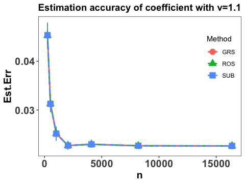
To comprehend the effect of sample size, we consider the same settings as in Yang et al. (2017) that and and conservatively, take for the three random sketch methods introduced in Section 4.2. Note that with the choice of , the time and store complexities reduce to and , respectively. Each scenario is replicated 50 times and the performance of the proposed method is evaluated by various measures, including the estimation accuracy of the linear coefficients, the integrated prediction error in terms of the slope function and the prediction error. Specifically, the estimation accuracy of the linear coefficients is evaluated by and Figure 1 shows the estimation accuracy of the coefficients with different choice of .
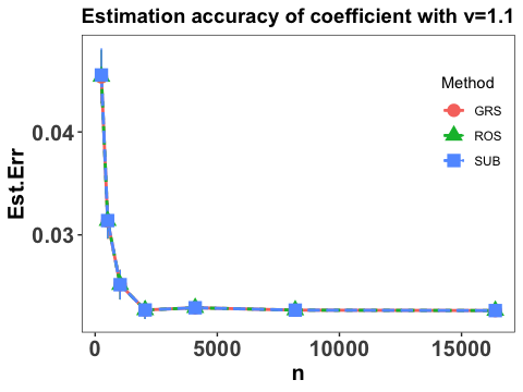

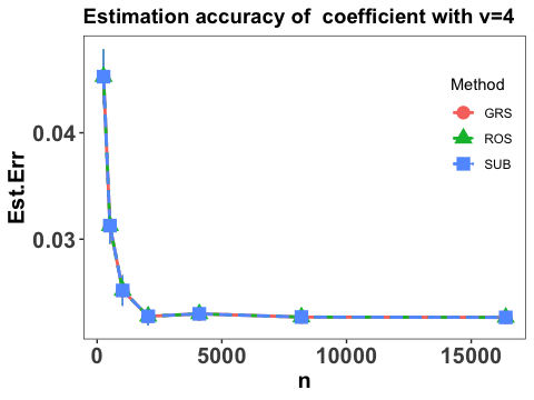
It is clear that the estimation error of the coefficients converges linearly as sample size increases and becomes stable when is sufficiently large, and the three employed sketch methods have similar performance. It is also interesting to notice that the convergence patterns under difference choice of are almost the same, which concurs with our theoretical findings that estimation of is not affected by the existence of nonparametric components in Theorems 1 and 3.
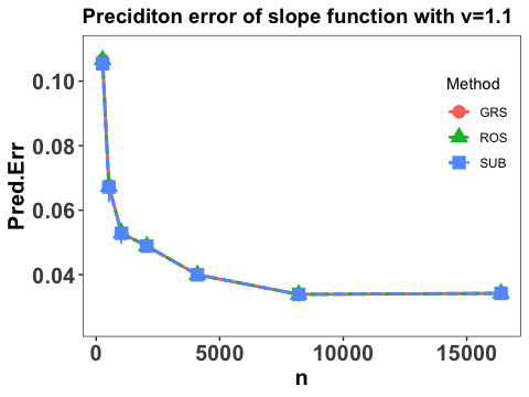
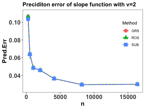
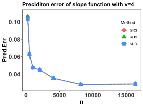
Let denotes an independent copy of and the integrated prediction error in terms of the slope function is reported by
The empirical expectation is evaluated by a testing sample with size and and the numerical performance are summarized in Figure 2.
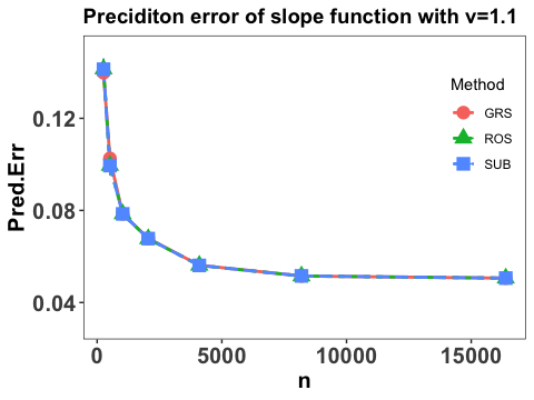
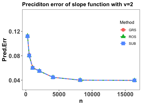
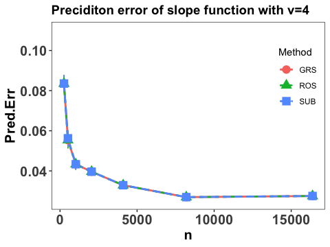
Note that Figure 2 suggests that the prediction error of the slope function converges at some polynomial rate as sample size , which agrees with our theoretical results in Section 3, and the three employed sketch methods yield similar numerical performance. Moreover, it can be seen that with the increase of the value of , the prediction error goes down, which also concurs with our theoretical findings in Theorems 2 and 3 that the faster decay rate of the eigenvalues, the smaller the prediction error.
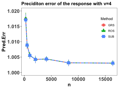
We also report the integrated prediction error of the response by calculating
The empirical expectation is also evaluated by a testing sample with size and the numerical performance are summarized in Figure 3.
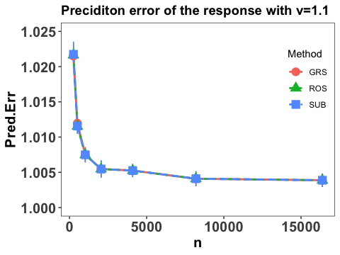
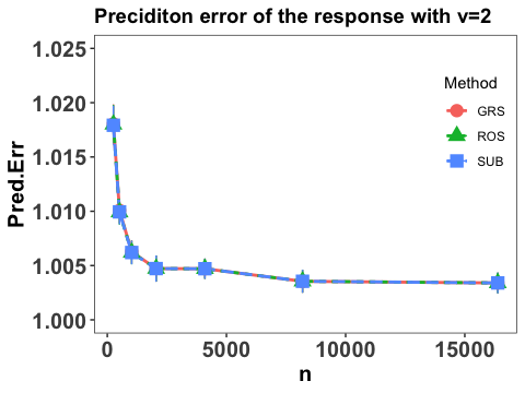
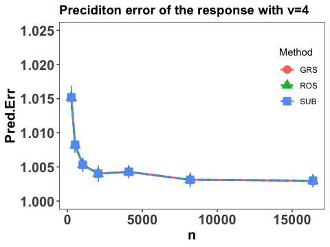
Clearly, we conclude that prediction error of the response converges at some polynomial rate as sample size and the prediction error becomes smaller with increases, which agrees with our theoretical results in Theorem 2. It is also interesting to point out that the three employed sketch methods yield similar numerical performance and the prediction errors tends to converge to 1, which is the variance of in the true modelling. This verifies the efficiency of the proposed estimation and the proper choice of .
Note that the numerical results in Example 2 where the eigenvalues are closely spaced are similar to those in the case with well-spaced eigenvalues in Example 1. Figure 4 shows the numerical performance under the closely spaced eigenvalues setting in Example 2.


6 Conclusion
This paper establishes the optimal minimax rate for the estimation of partially functional linear model (PFLM) under kernel-based and high dimensional setting. The optimal minimax rates of estimation is established by using various techniques in empirical process theory for analyzing kernel classes, and an efficient numerical algorithm based on randomized sketches of the kernel matrix is implemented to verify our theoretical findings.
Acknowledgments
Shaogao Lv’s research was partially supported by NSFC-11871277. Xin He’s research was supported in part by NSFC-11901375 and Shanghai Pujiang Program 2019PJC051. Junhui Wang’s research was supported in part by HK RGC Grants GRF-11303918 and GRF-11300919.
References
- Aronszajn (1950) N. Aronszajn. Theory of reporudcing kernels. Transactions of the American Mathematical Society, 68:337–404, 1950.
- Bickel et al. (2009) P. Bickel, Y. Ritov, and A. Tsybakov. Simultaneous analysis of lasso and dantzig selector. Annals of Statistics, 37:1705–1732, 2009.
- Bousquet (2002) O. Bousquet. A bennet concentration inequality and its application to suprema of empirical processes. Comptes Rendus Mathematique Academie des Sciences Paris, 334:495–550, 2002.
- Boyd and Vandenberghe (2004) S. Boyd and L. Vandenberghe. Convex Optimization. Cambridge University Press, Cambridge, 2004.
- Bühlmann and Van. de. Geer (2011) P. Bühlmann and S. Van. de. Geer. Statistics for High-Dimensional Data: Methods, Theory and Applications. Springer, Heidelberg, 2011.
- Cai and Yuan (2012) T. Cai and M. Yuan. Minimax and adaptive prediction for functional linear regression. Journal of the American Statistical Association, 107:1201–1216, 2012.
- Cardot et al. (2003) H. Cardot, F. Ferraty, and P. Sarda. Spline estimators for the functional linear model. Statistica Sinica, 13:571–591, 2003.
- Ferraty and Vieu (2006) F. Ferraty and P. Vieu. Nonparametric Functional Data Analysis: Theory and Practice. Springer, New York, 2006.
- Hall and Horowitz (2007) P. Hall and J. Horowitz. Methodology and convergence rates for functional linear regression. Annals of Statistics, 35:70–91, 2007.
- Kong et al. (2016) D. Kong, K. Xue, F. Yao, and H. Zhang. Partially functional linear regression in high dimensions. Biometrika, 103:1–13, 2016.
- Ledoux (1997) M. Ledoux. On talagrand’s deviation inequalities for product measures. Probability and Statistics, 1:63–87, 1997.
- Ledoux (2001) M. Ledoux. The Concentration of Measure Phenomenon (Mathematical Surveys and Monographs). American Mathematical Society, Providence, RI, 2001.
- Lu et al. (2014) Y. Lu, J. Du, and Z. Sun. Functional partially linear quantile regression model. Metrika, 77:17–32, 2014.
- Mahoney (2011) M. Mahoney. Randomized algorithms for matrices and data. Foundations and Trends in Machine Learning in Machine Learning, 3:1–54, 2011.
- Müller and Van de Geer (2015) P. Müller and S. Van de Geer. The partial linear model in high dimensions. Scandinavian Journal of Statistics, 42:580–608, 2015.
- Ramsay and Silverman (2005) J. Ramsay and B. Silverman. Functional Data Analysis. Springer, New York, 2005.
- Shin and Lee (2012) H. Shin and M. Lee. On prediction rate in partial functional linear regression. Journal of Multivariate Analysis, 103:93–106, 2012.
- Tsybakov (2009) A. Tsybakov. Introduction to Nonparametric Estimation. Springer, New York, 2009.
- Van. de. Geer (2000) S. Van. de. Geer. Emprical Processes in M-Estimation. Cambridge University Press, New York, 2000.
- Verzelen (2012) N. Verzelen. Minimax risks for sparse regressions: Ultra-high dimensional phenomenons. Electronic Journal of Statistics, 6:38––90, 2012.
- Yang and Barron (1999) Y. Yang and A. Barron. Information-theoretic determination of minimax rates of convergence. Annals of Statistics, 27:1564–1599, 1999.
- Yang et al. (2017) Y. Yang, M. Pilanci, and M. Wainwright. Randomized sketches for kernels: fast and optimal non-parametric regression. Annals of Statistics, 45:991–1023, 2017.
- Yu et al. (2019) Z. Yu, M. Levine, and G. Cheng. Minimax optimal estimation in partially linear additive models under high dimension. Bernoulli, 25:1289–1325, 2019.
- Yuan and Cai (2010) M. Yuan and T. Cai. A reproducing kernel hilbert space approach to functional linear regression. Annals of Statistics, 38:3412–3444, 2010.
- Zhu et al. (2014) H. Zhu, F. Yao, and H. Zhang. Structured functional additive regression in reproducing kernel hilbert spaces. Journal of the Royal Statistical Society, Series B, 76:581–603, 2014.