This paper was converted on www.awesomepapers.org from LaTeX by an anonymous user.
Want to know more? Visit the Converter page.

Kernel-based measures of association between inputs and outputs using ANOVA

Matieyendou Lamboni111Corresponding author: matieyendou.lamboni[at]gmail.com/univ-guyane.fr, 19/11/2023 University of Guyane, Department DFRST, 97346 Cayenne, French Guiana, France 228-UMR Espace-Dev, University of Guyane, University of Réunion, IRD, University of Montpellier, France.
Abstract

ANOVA decomposition of function with random input variables provides ANOVA functionals (AFs), which contain information about the contributions of the input variables on the output variable(s). By embedding AFs into an appropriate reproducing kernel Hilbert space regarding their distributions, we propose an efficient statistical test of independence between the input variables and output variable(s). The resulting test statistic leads to new dependent measures of association between inputs and outputs that allow for i) dealing with any distribution of AFs, including the Cauchy distribution, ii) accounting for the necessary or desirable moments of AFs and the interactions among the input variables. In uncertainty quantification for mathematical models, a number of existing measures are special cases of this framework. We then provide unified and general global sensitivity indices and their consistent estimators, including asymptotic distributions. For Gaussian-distributed AFs, we obtain Sobol’ indices and dependent generalized sensitivity indices using quadratic kernels.

keywords:
Dimension reduction , Independence tests , Kernel methods , Reducing uncertainties , Non-independent input variables

1 Introduction

In statistical modeling and data analysis, symmetric measures of dependence for random vectors such as the Pearson correlation ([1]); the Spearman correlation; the Kendall correlation; the canonical correlation coefficient ([2, 3]); the RV coefficient for two random vectors ([4]); the maximum mean discrepancy ([5, 6, 7]), including the energy distance ([8]); the Hilbert-Schmidt independence criterion ([9, 10, 11]), including the distance correlation ([12, 13]) and a recent correlation coefficient ([14]) have been used by different communities for testing whether two random vectors are independent or not, and then for measuring the dependence between such random vectors. Drawbacks, advantages and links between such dependent measures can be found in [15, 16, 11, 17] for instance.

The above dependent measures do not require any function linking both random vectors. In presence of a mathematical model or a black box function of the form Y=f(𝐗)Y=f(\mathbf{X}), where 𝐗:=(X1,,Xd)\mathbf{X}:=(X_{1},\ldots,X_{d}) are the model inputs with known probability distributions and YY is the model output, such measures can still be used for testing the independence between the model output Y=f(𝐗)Y=f(\mathbf{X}) and some inputs such as X1X_{1}. Such a problem occurs in computer experiments where a natural or human induced phenomenon is represented by complex computer code with numerous input variables ([18]). For dimension reduction, it is relevant to identify unessential variables by means of different criteria such as statistical tests of independence or the variance-based sensitivity indices (SIs) ([19, 20, 21, 22, 23]), which were developed in the framework of the statistical theory called ANOVA ([24, 25, 26, 19]).

Formally, the above dependent measures between f(𝐗)f(\mathbf{X}) and X1X_{1} rely on the test statistic of the form T(f(𝐗),X1)T(f(\mathbf{X}),X_{1}) or T(f(𝐗),h(X1))T(f(\mathbf{X}),h(X_{1})) with T,hT,\,h some given functions. When a statistical test reveals that the random variables f(𝐗)f(\mathbf{X}) and X1X_{1} are dependent, the associated test statistic usually serves as a reasonable measure of the association between both variables. While this crude dependent measure is relevant for screening input variables in some cases, it may be not satisfying for ranking input variables because it involves only the inputs of interest and the output or the output and its conditional expectation given the inputs of interest ([27, 28, 29, 30]). Moreover, it i) may result in dealing with transformations of the model output rather than using YY ([31]); ii) may include undesirable effects or complicate the problem ([31, 32]); iii) ignores the asymmetric role of the model inputs and output. For instance, the MMD-based indices result in using ϕ(𝐘)\phi(\mathbf{Y}) as outputs with ϕ\phi some given functions a.k.a. feature maps (see [33]). In the same sense, the HSIC-based indices proposed in [33] result in working with transformations of the original inputs and output, as the HSIC requires defining one kernel on the inputs and another one on the outputs ([34]).

It is known that ANOVA remains an important step in exploratory and confirmatory analysis of model ([35]), and it relies on direct use of the model output(s) and inputs. The well-known ANOVA-like decomposition of f(𝐗)f(\mathbf{X}) with independent variables 𝐗\mathbf{X} can be written as follows ([24, 25, 26, 19, 36, 37]):

f(𝐗)=v{1,,d}fv(𝐗v)=𝔼[f(𝐗)]+f1tot(𝐗)+f1(X2,,Xd),f(\mathbf{X})=\sum_{\begin{subarray}{c}v\subseteq\{1,\ldots,d\}\end{subarray}}f_{v}\left(\mathbf{X}_{v}\right)=\mathbb{E}\left[f(\mathbf{X})\right]+f_{1}^{tot}(\mathbf{X})+f_{\sim 1}(X_{2},\ldots,X_{d})\,, (1)

where 𝐗v\mathbf{X}_{v} is a subset of the model inputs whose subscripts belong to vv; and f1tot(𝐗):=v{1,,d}v{1}fv(𝐗v)f_{1}^{tot}(\mathbf{X}):=\sum_{\begin{subarray}{c}v\subseteq\{1,\ldots,d\}\\ v\cap\{1\}\neq\emptyset\end{subarray}}f_{v}\left(\mathbf{X}_{v}\right) denotes the total ANOVA functional (AF) of X1X_{1}. The FANOVA decomposition of functions with non-independent variables is similar thanks to dependency models of dependent variables (see Section 2 and [38, 39, 40]). ANOVA functionals are random variables, which contain the primary information about the contributions of the input variables on the output variable. In view of Equation (1), f(𝐗)f(\mathbf{X}) does not dependent on X1X_{1} whenever the total AF follows the Dirac probability measure δ𝟎\delta_{\mathbf{0}}, that is, f1tot(𝐗)=0f_{1}^{tot}(\mathbf{X})=0 almost surely (a.s.) (see [41] for independent variables and Lemma 1 in general).

The aim of this paper is to propose a new dependent measure between the model inputs and output(s) that is more comprehensive and much flexible to account for the necessary or desirable statistical properties of AFs (e.g., higher-order moments, the Cauchy and heavy tailed distributions, asymmetric distributions) and the interactions among the input variables. The proposed dependent measure relies on the properties of AFs such as the independence criterion f1tot(𝐗)=0a.s.f_{1}^{tot}(\mathbf{X})=0\;a.s. and the reproducing kernel Hilbert space (RKHS) ([42, 43, 44]). The RKHS theory offers a flexible framework for precise statistical inference of probability distributions ([6, 34, 16]), and it is crucial for conducting independence tests that account for the necessary or sufficient or desirable statistical properties of distributions ([9, 6, 34, 45, 46, 32]). The proposed dependent measure leads to provide the first-order and total kernel-based sensitivity indices, and its empirical expression is used for deriving a test statistic for testing the independence between the model inputs and output(s).

This paper is organized as follows: Section 2 deals with AFs and their statistical properties in terms of their ability to assess the effects of the input variables on the model output(s). Such properties enable the formulation of the initial null hypothesis for the independence test between input variables and the model output(s) and equivalent null hypothesis such as the variance 𝕍[f1tot(𝐗)]=0\mathbb{V}\left[f_{1}^{tot}(\mathbf{X})\right]=0. Most of variance-based SIs rely on that null hypothesis for performing dimension reduction. Indeed, 𝕍[f1tot(𝐗)]\mathbb{V}\left[f_{1}^{tot}(\mathbf{X})\right] represents the non-normalized total SI of X1X_{1}.
Since the associated alternative hypothesis is sufficient for AFs that are Gaussian-distributed and the Cauchy distribution does not have the variance, Section 3 is devoted to develop equivalent null hypothesis for the independence test by embedding AFs into an appropriate RKHS regarding their distributions. Moreover, as a given kernel can help for working with specific moments ([32]), we also provide the set of distribution-free kernels that guarantee the equivalent null hypothesis for the independence test between the model inputs and output(s). Section 4 presents a statistical test that leads to an interesting measure of association between inputs and output(s). In Section 5, we formally introduce our empirical dependent measure and the associated test statistic. We also provide and study kernel-based SIs. We provide analytical and numerical results in Section 8 and conclude this work in Section 9.

General notations

For an inetegr d>1d>1, dd input variables 𝐗:=(X1,,Xd)\mathbf{X}:=(X_{1},\,\ldots,\,X_{d}) and u{1,,d}u\subseteq\{1,\,\ldots,\,d\}, we use 𝐗u:=(Xj,ju)\mathbf{X}_{u}:=(X_{j},\forall\,j\in u), 𝐗u:=(Xj,j{1,,d}u)\mathbf{X}_{\sim u}:=(X_{j},\forall\,j\in\{1,\,\ldots,\,d\}\setminus u) and |u||u| for the number of elements in uu. Thus, we have the partition 𝐗=(𝐗u,𝐗u)\mathbf{X}=(\mathbf{X}_{u},\,\mathbf{X}_{\sim u}). We also use 𝐑=d𝐗\mathbf{R}\stackrel{{\scriptstyle d}}{{=}}\mathbf{X} to say that 𝐑\mathbf{R} and 𝐗\mathbf{X} have the same cumulative distribution function (CDF).

2 Theoretical properties of ANOVA functionals of (in)-dependent inputs

In this section, we provide the properties of ANOVA functionals for functions with non-independent variables. Such properties serve as the initial null hypothesis for testing the independence between the random input variables and output variables. For the sequel of generality, consider a vector-valued function f:dnf:\mathbb{R}^{d}\to\mathbb{R}^{n}, which includes a dd-dimensional random vector 𝐗\mathbf{X} as inputs and provides nn outputs given by f(𝐗)f(\mathbf{X}). We are interested in measuring the association between the following two random vectors: f(𝐗)f(\mathbf{X}) and 𝐗u\mathbf{X}_{u} with u{1,,d}u\subseteq\{1,\ldots,d\} and uu\neq\emptyset, keeping in mind the asymmetric role between both random vectors.

For any distribution of 𝐗\mathbf{X}, we are able to model 𝐗\mathbf{X} as follows ([47, 38, 40, 39]):

𝐗u=dru(𝐗u,𝐙);\mathbf{X}_{\sim u}\stackrel{{\scriptstyle d}}{{=}}r_{u}\left(\mathbf{X}_{u},\mathbf{Z}\right)\,; (2)

where rur_{u} is a function; 𝐙\mathbf{Z} is a random vector of d|u|d-|u| independent variables, and 𝐗u\mathbf{X}_{u} is independent of 𝐙\mathbf{Z}. Note that when 𝐗\mathbf{X} is consisted of independent variables, the dependency function in (2) comes down to 𝐗u:=dru(𝐙)\mathbf{X}_{\sim u}\stackrel{{\scriptstyle d}}{{:=}}r_{u}\left(\mathbf{Z}\right). Composing ff by the function rur_{u} in (2) yields

g(𝐗u,𝐙):=df(𝐗u,ru(𝐗u,𝐙)).g(\mathbf{X}_{u},\mathbf{Z})\stackrel{{\scriptstyle d}}{{:=}}f(\mathbf{X}_{u},r_{u}(\mathbf{X}_{u},\,\mathbf{Z}))\,. (3)

In view of Equation (3), the function gg includes two independent random vectors (i.e., 𝐗u\mathbf{X}_{u} and 𝐙\mathbf{Z}) as inputs, and it provides nn outputs sharing the distribution of f(𝐗)f(\mathbf{X}). For independent variables 𝐗\mathbf{X}, we can see that g(𝐗u,𝐙)=f(𝐗u,ru(𝐙))=df(𝐗u,𝐗u)g(\mathbf{X}_{u},\mathbf{Z})=f(\mathbf{X}_{u},r_{u}(\mathbf{Z}))\stackrel{{\scriptstyle d}}{{=}}f(\mathbf{X}_{u},\mathbf{X}_{\sim u}). For the sequel of generality, we are going to use g(𝐗u,𝐙)g(\mathbf{X}_{u},\mathbf{Z}) in what follows, which comes down to f(𝐗u,𝐗u)f(\mathbf{X}_{u},\mathbf{X}_{\sim u}) when the inputs are independent. As a matter of fact, we can always claim that

(A1) our function of interest gg includes two independent random vectors: 𝐗u\mathbf{X}_{u} and 𝐙\mathbf{Z}.

Note that (A1) is not theoretically or practically restrictive because it is always satisfied thanks to dependency models (see (2)).

2.1 ANOVA functionals

Under (A1), the Hoeffding decomposition of g(𝐗u,𝐙)g(\mathbf{X}_{u},\mathbf{Z}) is given by ([24, 25, 26, 19])

g(𝐗u,𝐙)=𝔼𝐗u,𝐙[g(𝐗u,𝐙)]+gu(𝐗u)+gu(𝐙)+gu,u(𝐗u,𝐙),g(\mathbf{X}_{u},\mathbf{Z})=\mathbb{E}_{\mathbf{X}_{u},\mathbf{Z}}\left[g(\mathbf{X}_{u},\mathbf{Z})\right]+g_{u}(\mathbf{X}_{u})+g_{\sim u}(\mathbf{Z})+g_{u,\sim u}(\mathbf{X}_{u},\mathbf{Z})\,,

where 𝔼𝐗u,𝐙[g(𝐗u,𝐙)]=:𝔼[g(𝐗u,𝐙)]\mathbb{E}_{\mathbf{X}_{u},\mathbf{Z}}\left[g(\mathbf{X}_{u},\mathbf{Z})\right]=:\mathbb{E}\left[g(\mathbf{X}_{u},\mathbf{Z})\right] is the expectation taking w.r.t. 𝐗u,𝐙\mathbf{X}_{u},\mathbf{Z};

gu(𝐗u):=𝔼𝐙[g(𝐗u,𝐙)]𝔼[g(𝐗u,𝐙)];gu(𝐙):=𝔼𝐗u[g(𝐗u,𝐙)]𝔼[g(𝐗u,𝐙)],g_{u}(\mathbf{X}_{u}):=\mathbb{E}_{\mathbf{Z}}\left[g(\mathbf{X}_{u},\mathbf{Z})\right]-\mathbb{E}\left[g(\mathbf{X}_{u},\mathbf{Z})\right];\,\quad g_{\sim u}(\mathbf{Z}):=\mathbb{E}_{\mathbf{X}_{u}}\left[g(\mathbf{X}_{u},\mathbf{Z})\right]-\mathbb{E}\left[g(\mathbf{X}_{u},\mathbf{Z})\right]\,,
gu,u(𝐗u,𝐙):=g(𝐗u,𝐙)gu(𝐗u)gu(𝐙)+𝔼[g(𝐗u,𝐙)].g_{u,\sim u}(\mathbf{X}_{u},\mathbf{Z}):=g(\mathbf{X}_{u},\mathbf{Z})-g_{u}(\mathbf{X}_{u})-g_{\sim u}(\mathbf{Z})+\mathbb{E}\left[g(\mathbf{X}_{u},\mathbf{Z})\right]\,.

The first-order and total AFs of 𝐗u\mathbf{X}_{u} are defined as follows: ([23, 48, 38, 39, 49, 40])

gufo(𝐗u):=𝔼𝐙[g(𝐗u,𝐙)]𝔼[g(𝐗u,𝐙)]=gu(𝐗u),g^{fo}_{u}(\mathbf{X}_{u}):=\mathbb{E}_{\mathbf{Z}}\left[g(\mathbf{X}_{u},\mathbf{Z})\right]-\mathbb{E}\left[g(\mathbf{X}_{u},\mathbf{Z})\right]=g_{u}(\mathbf{X}_{u})\,,
gutot(𝐗u,𝐙):=g(𝐗u,𝐙)𝔼𝐗u[g(𝐗u,𝐙)].g^{tot}_{u}(\mathbf{X}_{u},\mathbf{Z}):=g(\mathbf{X}_{u},\mathbf{Z})-\mathbb{E}_{\mathbf{X}_{u}}\left[g(\mathbf{X}_{u},\mathbf{Z})\right]\,.

It is worth noting that both AFs are zero-mean and nn-dimensional random vectors, which are directly based on the model outputs. We also have the following relationship:

gufo(𝐗u)=𝔼𝐙[gutot(𝐗u,𝐙)].g^{fo}_{u}(\mathbf{X}_{u})=\mathbb{E}_{\mathbf{Z}}\left[g^{tot}_{u}(\mathbf{X}_{u},\mathbf{Z})\right]\,. (4)

Recall that AFs contain the primary information about the contribution of the random vector 𝐗u\mathbf{X}_{u} to the model outputs given by g(𝐗u,𝐙)=df(𝐗)g(\mathbf{X}_{u},\mathbf{Z})\stackrel{{\scriptstyle d}}{{=}}f(\mathbf{X}). The main interesting property of AFs is derived in Lemma 1.

Lemma 1

Under (A1), f(𝐗)=dg(𝐗u,𝐙)f(\mathbf{X})\stackrel{{\scriptstyle d}}{{=}}g(\mathbf{X}_{u},\mathbf{Z}) is independent of 𝐗u\mathbf{X}_{u} iff

gutot(𝐗u,𝐙)=𝟎a.s..g^{tot}_{u}(\mathbf{X}_{u},\mathbf{Z})=\mathbf{0}\;\;a.s.\,.

Proof.  See Appendix A.

\Box

From Lemma 1, it is clear that the total AF gutot(𝐗u,𝐙)g^{tot}_{u}(\mathbf{X}_{u},\mathbf{Z}) is sufficient for fully characterizing the independence between f(𝐗)f(\mathbf{X}) and 𝐗u\mathbf{X}_{u}. We then formulate the initial test hypotheses of independence as follows:

H0:gutot(𝐗u,𝐙)=𝟎a.s.Vs.H1:gutot(𝐗u,𝐙)𝟎a.s..H_{0}:\;g^{tot}_{u}(\mathbf{X}_{u},\mathbf{Z})\stackrel{{\scriptstyle}}{{=}}\mathbf{0}\;a.s.\,\qquad\mbox{Vs.}\qquad H_{1}:\;g^{tot}_{u}(\mathbf{X}_{u},\mathbf{Z})\stackrel{{\scriptstyle}}{{\neq}}\mathbf{0}\;a.s.\,.

While the null hypothesis is equivalent to 𝕍[gutot(𝐗u,𝐙)]=𝖮\mathbb{V}\left[g^{tot}_{u}(\mathbf{X}_{u},\mathbf{Z})\right]=\mathsf{O}, with 𝖮\mathsf{O} a null matrix, its alternative hypothesis given by 𝕍[gutot(𝐗u,𝐙)]𝖮\mathbb{V}\left[g^{tot}_{u}(\mathbf{X}_{u},\mathbf{Z})\right]\neq\mathsf{O} may be not satisfying because it does not account for higher-order moments. Moreover, this null hypothesis implicitly requires the existence of the variance-covariance of AFs, which is not the case for the Cauchy distribution for instance. Therefore, we need a dependent measure that accounts for sufficient or desirable higher-order moments for a given distribution of gutot(𝐗u,𝐙)g^{tot}_{u}(\mathbf{X}_{u},\mathbf{Z}). Since the total AF is a random vector, we may use the probability metrics based on the difference between distribution functions or the Wasserstein metric or the kernel methods for making such comparisons. Significant discussions about such metrics and kernel methods can be found in [16]. To develop our dependent measure, we are going to use the kernel methods that are much flexible for including specific moments of AFs.

2.2 Embedding ANOVA functionals into a RKHS

To build a statistical test that i) leads to interesting dependent measures, ii) is much flexible for explicitly including specific moments, iii) is able to distinguish two different distributions, AFs are going to be embedded into a RKHS or feature spaces according to their distributions ([44, 6, 34]).

Definition 1

(Aronszajn, 1950) Let 𝒳\mathcal{X} be an arbitrary space, \mathcal{H} be an Hilbert space endowed with the inner product ,\left<\cdot,\,\cdot\right>. The functions

(i) ϕ:𝒳\phi:\mathcal{X}\to\mathcal{H} is called a feature map;

(ii) k:𝒳×𝒳k:\mathcal{X}\times\mathcal{X}\to\mathbb{R} given by k(r,r)=ϕ(r),ϕ(r)=:k(,r),k(,r)k(r,r^{\prime})=\left<\phi(r),\,\phi(r^{\prime})\right>=:\left<k(\cdot,r),\,k(\cdot,r^{\prime})\right> is called a valid kernel.

A kernel k𝒦k\in\mathcal{K} is said centered at r0r_{0} when k(,r0)=0k(\cdot,r_{0})=0. Given a kernel k(r,r)k(r,r^{\prime}), we can construct a new kernel that is centered at r0r_{0} as follows ([11]):

kc(r,r):=k(r,r)+k(r0,r0)k(r,r0)k(r0,r).k_{c}\left(r,r^{\prime}\right):=k\left(r,r^{\prime}\right)+k\left(r_{0},r_{0}\right)-k\left(r,r_{0}\right)-k\left(r_{0},r^{\prime}\right)\,.

For a nn-dimensional random vector 𝐆\mathbf{G} having FF as CDF (i.e., 𝐆F\mathbf{G}\sim F) such as AFs, the transformation k(,𝐆)k(\cdot,\mathbf{G}) aims at embedding this random vector into a RKHS induced by k(𝐆,𝐆)k(\mathbf{G},\mathbf{G}^{\prime}) with 𝐆\mathbf{G}^{\prime} an i.i.d. copy of 𝐆\mathbf{G}. Linear statistics in the new RKHS such as the mean element account for all the moments or desirable moments of 𝐆\mathbf{G} depending on the kernel kk ([6, 34, 7]). For embedding AFs into a RKHS and working with the mean element (see Definition 2), we use 𝒫B\mathcal{P}_{B} for the set of Borel probability distributions and define the set of AFs distributions as follows:

:={F𝒫B:gutot(𝐗u,𝐙)Forgufo(𝐗u)F,u{1,,d}}.\mathcal{F}:=\left\{F\in\mathcal{P}_{B}:\,g^{tot}_{u}(\mathbf{X}_{u},\mathbf{Z})\sim F\quad\mbox{or}\quad g^{fo}_{u}(\mathbf{X}_{u})\sim F,\;\;\forall\,u\subseteq\{1,\ldots,d\}\right\}\,.

The class of distributions \mathcal{F} is adequate for manipulating AFs. For a valid and measurable kernel, we assume that

(A2): 𝔼[k(𝐆,𝐆)]<\mathbb{E}\left[\sqrt{k(\mathbf{G},\mathbf{G})}\right]<\leavevmode\nobreak\ \infty for all 𝐆F\mathbf{G}\sim F\in\mathcal{F}.

Definition 2

([6, 7]). Consider a kernel kk and 𝐆F\mathbf{G}\sim F\in\mathcal{F}.
The map 𝐆𝔼F[k(,𝐆)]\mathbf{G}\mapsto\mathbb{E}_{F}\left[k(\cdot,\mathbf{G})\right] is called a mean feature map; and μF(𝐆):=𝔼F[k(,𝐆)]\mu_{F}(\mathbf{G}):=\mathbb{E}_{F}\left[k(\cdot,\mathbf{G})\right] is called the mean element.

Generally, the feature map is used to embed 𝐆\mathbf{G} into a higher dimensional random vectors so as to include all type of information about the data. Characteristic kernels aim to accomplish such tasks ([50, 6, 45, 46, 51]).

Definition 3

([6, 45]) Conisder two random vectors 𝐆1F,𝐆2H\mathbf{G}_{1}\sim F,\;\mathbf{G}_{2}\sim H.
A measurable kernel kk is said characteristic if the mean feature map is one to one:

μF(𝐆1)=μH(𝐆2)F=H(i.e.,𝐆1=d𝐆2).\mu_{F}(\mathbf{G}_{1})=\mu_{H}(\mathbf{G}_{2})\Longleftrightarrow F=H\quad(i.e.,\mathbf{G}_{1}\stackrel{{\scriptstyle d}}{{=}}\mathbf{G}_{2})\,.

Taking the distance between μF(𝐆1)\mu_{F}(\mathbf{G}_{1}) and μH(𝐆2)\mu_{H}(\mathbf{G}_{2}) leads to the maximum mean discrepancy (MMD), that is, MMD2(𝐆1,𝐆2):=μF(𝐆1)μH(𝐆2)2MMD^{2}(\mathbf{G}_{1},\mathbf{G}_{2}):=\left|\left|\mu_{F}(\mathbf{G}_{1})-\mu_{H}(\mathbf{G}_{2})\right|\right|_{\mathcal{H}}^{2} ([5, 6, 7]). Note that the centered kernel kck_{c} associated with a valid kernel kk is a characteristic kernel if and only if kk is a characteristic one ([11]).

Thus, the mean element associated with a characteristic kernel uniquely determines a probability distribution. This interesting property gives us the ability to use the mean element for fully characterizing the distribution of AFs. It is to be noted that characteristic kernels for specific class of distributions such as the class of Gaussian distributions can be defined as well. Thus, characteristic kernels on \mathcal{F} are sufficient for distinguishing different AFs. For instance, while a test statistic that can distinguish the first two moments is sufficient for a class of Gaussian distributions, the mean element of the form 𝔼[e𝐆Tt]\mathbb{E}\left[e^{\mathbf{G}^{T}t}\right] with tnt\in\mathbb{R}^{n}, which generalizes the notion of moment-generating function in probability, allows for distinguishing all the moments of a probability distribution.

3 Kernels for equivalent null hypothesis

This section provides a set of kernels that ensure the equivalent criterion of independence between the input variables 𝐗u\mathbf{X}_{u} and the model outputs. Recall that the null hypothesis 𝕍[gutot(𝐗u,𝐙)]=𝖮\mathbb{V}\left[g^{tot}_{u}(\mathbf{X}_{u},\mathbf{Z})\right]=\mathsf{O} is an equivalent criterion of independence, and it is also obtained using the quadratic kernel, that is, k2(𝐫,𝐫)=𝐫,𝐫n2k_{2}\left(\mathbf{r},\mathbf{r}^{\prime}\right)=\left<\mathbf{r},\,\mathbf{r}^{\prime}\right>^{2}_{\mathbb{R}^{n}}. Indeed, if we use 𝐗u,𝐙\mathbf{X}_{u}^{\prime},\mathbf{Z}^{\prime} for i.i.d. copies of 𝐗u,𝐙\mathbf{X}_{u},\mathbf{Z}, we can check that

𝔼[k2(gutot(𝐗u,𝐙),gutot(𝐗u,𝐙))]=0𝕍[gutot(𝐗u,𝐙)]=𝖮.\mathbb{E}\left[k_{2}\left(g^{tot}_{u}(\mathbf{X}_{u},\mathbf{Z}),\,g^{tot}_{u}(\mathbf{X}_{u}^{\prime},\mathbf{Z}^{\prime})\right)\right]=0\Longleftrightarrow\mathbb{V}\left[g^{tot}_{u}(\mathbf{X}_{u},\mathbf{Z})\right]=\mathsf{O}\,.

It is worth noting that kernels of the form k2p(𝐫,𝐫)=𝐫,𝐫n2pk_{2p}\left(\mathbf{r},\mathbf{r}^{\prime}\right)=\left<\mathbf{r},\,\mathbf{r}^{\prime}\right>^{2p}_{\mathbb{R}^{n}} for integer p>0p>0 lead to an equivalent null hypothesis of independence, although such kernels are not characteristic in general. Since some kernels do not ensure the independence criterion, let us start with the following definitions thanks to Lemma 1. Namely, we use 𝒦\mathcal{K} for the set of valid and measurable kernels; HH for the CDF of the Dirac probability measure δ{𝟎}\delta_{\{\mathbf{0}\}}.

Definition 4

A kernel k𝒦k\in\mathcal{K} is said to be an equivalent kernel for the independence test between 𝐗u\mathbf{X}_{u} and g(𝐗u,𝐙)g(\mathbf{X}_{u},\mathbf{Z}) whenever

𝔼[k(gutot(𝐗u,𝐙),gutot(𝐗u,𝐙))]k(𝟎,𝟎)=0gutot(𝐗u,𝐙)=𝟎a.s..\mathbb{E}\left[k\left(g^{tot}_{u}(\mathbf{X}_{u},\mathbf{Z}),\,g^{tot}_{u}(\mathbf{X}_{u}^{\prime},\mathbf{Z}^{\prime})\right)\right]-k(\mathbf{0},\mathbf{0})=0\,\Longrightarrow\,g^{tot}_{u}(\mathbf{X}_{u},\mathbf{Z})=\mathbf{0}\;a.s.\;\,. (5)

The equivalence used in Definition 4 is guaranteed by Lemma 1. For a centered kernel at 𝟎\mathbf{0} (i.e., k¯\bar{k}), the left term of Equation (5) becomes 𝔼[k¯(gutot(𝐗u,𝐙),gutot(𝐗u,𝐙))]= 0\mathbb{E}\left[\bar{k}\left(g^{tot}_{u}(\mathbf{X}_{u},\mathbf{Z}),\,g^{tot}_{u}(\mathbf{X}_{u}^{\prime},\mathbf{Z}^{\prime})\right)\right]=\leavevmode\nobreak\ 0.

To construct the set of equivalent kernels for the independence test, consider the following set of kernels:

𝒦E:={k𝒦:𝔼𝐆F,𝐆F[k¯(𝐆,𝐆)]=0F=H,For𝔼(𝐆,𝐆)ν[k(𝐆,𝐆)]=0ν=0,ν=FFHH}.\mathcal{K}_{E}:=\left\{k\in\mathcal{K}:\,\begin{array}[]{c}\,\mathbb{E}_{\mathbf{G}\sim F,\mathbf{G}^{\prime}\sim F}\left[\bar{k}(\mathbf{G},\mathbf{G}^{\prime})\right]=0\Rightarrow F=H,\;\forall\,F\in\mathcal{F}\\ \mbox{or}\\ \mathbb{E}_{(\mathbf{G},\,\mathbf{G}^{\prime})\sim\nu}\left[k(\mathbf{G},\mathbf{G}^{\prime})\right]=0\Rightarrow\nu=0,\;\forall\,\nu=F\otimes F-H\otimes H\end{array}\right\}\,. (6)

We can check that 𝒦E\mathcal{K}_{E} contains quadratic kernels that are centered at 𝟎\mathbf{0}, and we are going to see that it contains some well-known characteristic kernels. Lemma 2 gives interesting properties of 𝒦E\mathcal{K}_{E} regarding the null hypothesis.

Lemma 2

Let k𝒦Ek\in\mathcal{K}_{E} and assume that (A1) and (A2) hold. Then,

kk is an equivalent kernel for the independence test between 𝐗u\mathbf{X}_{u} and g(𝐗u,𝐙)g(\mathbf{X}_{u},\mathbf{Z}).

Proof.  See Appendix B.

\Box

Lemma 2 shows that the set 𝒦E\mathcal{K}_{E} given by (6) contains equivalent kernels for the independence criterion whatever are the distributions of the model outputs and total AFs. Despite 𝒦E\mathcal{K}_{E} is not exhaustive, Lemma 3 shows its richness. To that end, consider the famous radial-based characteristic kernels on n×n\mathbb{R}^{n}\times\mathbb{R}^{n} given by

k(𝐫,𝐫):=ei(𝐫𝐫)T𝐰𝑑Λ(𝐰),k(\mathbf{r},\mathbf{r}^{\prime}):=\int e^{-i(\mathbf{r}-\mathbf{r}^{\prime})^{T}\mathbf{w}}\,d\Lambda(\mathbf{w})\,,

where Λ\Lambda is a positive and bounded Borel measure with the support Supp(Λ)=nSupp(\Lambda)=\mathbb{R}^{n}.

Lemma 3

Let k,k¯𝒦k,\,\bar{k}\in\mathcal{K} and assume (A1)-(A2) hold.

    (i) If kk is a characteristic kernel, then the centered kernel k¯𝒦E\bar{k}\in\mathcal{K}_{E}.

    (ii) If kk is a radial-based characteristic kernel, then k𝒦Ek\in\mathcal{K}_{E}.

Proof.  See Appendix C.

\Box

Kernels k¯\bar{k} of Point (i) in Lemma 3 lead to a comparison between the distributions of the total AF and the Dirac measure using the maximum mean discrepancy (see Section 6.2). Thus, Point (ii) offers other possibilities that allow for working with non-centered and characteristic kernels such as Gaussian kernels.

Example of equivalent kernels for the independence test

  • 1.

    A class of distance-induced characteristic kernels that are already centered at 𝟎\mathbf{0} contains the following kernels ([11]):

    kdα(𝐫,𝐫):=12(||𝐫||2α+||𝐫||2α||𝐫𝐫||2α),α]0, 2[.k_{d}^{\alpha}(\mathbf{r},\mathbf{r}^{\prime}):=\frac{1}{2}\left(\left|\left|\mathbf{r}\right|\right|_{2}^{\alpha}+\left|\left|\mathbf{r}^{\prime}\right|\right|_{2}^{\alpha}-\left|\left|\mathbf{r}-\mathbf{r}^{\prime}\right|\right|_{2}^{\alpha}\right),\quad\forall\,\alpha\in]0,\,2[\,.
  • 2.

    Recall that kernels given by k2p(𝐫,𝐫):=𝐫,𝐫n2pk_{2p}(\mathbf{r},\mathbf{r}^{\prime}):=\left<\mathbf{r},\mathbf{r}^{\prime}\right>^{2p}_{\mathbb{R}^{n}} for any integer p1p\geq 1 belong to 𝒦E\mathcal{K}_{E}. Moreover, for any integer 2L<2\leq L<\infty and positive definite and diagonal matrix 𝒟d\mathcal{D}_{d}, kernels of the form k¯𝒟(𝐫,𝐫):=q=1L2(𝐫T𝒟q𝐫)q\bar{k}_{\mathcal{D}}(\mathbf{r},\mathbf{r^{\prime}}):=\sum_{q=1}^{L\geq 2}\left(\mathbf{r}^{T}\mathcal{D}_{q}\mathbf{r}^{\prime}\right)^{q} are in 𝒦E\mathcal{K}_{E}. Each kernel kq(𝐫,𝐫):=(𝐫T𝒟q𝐫)qk_{q}\left(\mathbf{r},\mathbf{r}^{\prime}\right):=\left(\mathbf{r}^{T}\mathcal{D}_{q}\mathbf{r}^{\prime}\right)^{q} is sufficient for incorporating the qthq^{th}-order moments of the total AF and all the correlations among the components of AFs. In general, we are able to incorporate all the moments by taking L+L\to+\infty, which leads to the exponential kernel, that is, ke(𝐫,𝐫)=eα𝐫,𝐫k_{e}(\mathbf{r},\mathbf{r^{\prime}})=e^{\alpha\left<\mathbf{r},\,\mathbf{r}^{\prime}\right>} with α>0\alpha>0.

  • 3.

    Finally, radial-based characteristic kernels such as Gaussian, Laplacian and the Cauchy kernels and their associated centered kernels belong to 𝒦E\mathcal{K}_{E}. Note that the Gaussian kernel is the normalized version of the exponential kernel.

4 New independence test and dependent measure between inputs and outputs

For testing the independence between g(𝐗u,𝐙)g\left(\mathbf{X}_{u},\mathbf{Z}\right) and 𝐗u\mathbf{X}_{u} and obtaining an interesting dependent measure when 𝐗u\mathbf{X}_{u} contribute to the outputs g(𝐗u,𝐙)g\left(\mathbf{X}_{u},\mathbf{Z}\right), we are going to use kernels that guarantee the equivalent null hypothesis of independence between these random vectors such as the set of kernels 𝒦E\mathcal{K}_{E}.

4.1 Test hypotheses and deviation mesaure from independence

For concise notations, we use 𝐆utot:=gutot(𝐗u,𝐙)\mathbf{G}^{tot}_{u}\stackrel{{\scriptstyle}}{{:=}}g^{tot}_{u}\left(\mathbf{X}_{u},\mathbf{Z}\right), 𝐆utot:=gutot(𝐗u,𝐙)\mathbf{G}^{tot^{\prime}}_{u}\stackrel{{\scriptstyle}}{{:=}}g^{tot}_{u}\left(\mathbf{X}_{u}^{\prime},\mathbf{Z}^{\prime}\right), and we see that 𝐆utot\mathbf{G}^{tot^{\prime}}_{u} is an i.i.d. copy of 𝐆utot\mathbf{G}^{tot}_{u}. For a real q>0q>0, k𝒦Ek\in\mathcal{K}_{E}, the generic test hypotheses are formally given by

H0:|𝔼[k(𝐆utot,𝐆utot)]k(𝟎,𝟎)|q=0VsH1:|𝔼[k(𝐆utot,𝐆utot)]k(𝟎,𝟎)|q0.H_{0}^{\prime}:\left|\mathbb{E}\left[k\left(\mathbf{G}^{tot}_{u},\mathbf{G}^{tot^{\prime}}_{u}\right)\right]-k(\mathbf{0},\mathbf{0})\right|^{q}=0\quad\mbox{Vs}\quad H_{1}^{\prime}:\left|\mathbb{E}\left[k\left(\mathbf{G}^{tot}_{u},\mathbf{G}^{tot^{\prime}}_{u}\right)\right]-k(\mathbf{0},\mathbf{0})\right|^{q}\neq 0\,.

If we use FTuF_{T_{u}}\in\mathcal{F} for the CDF of 𝐆utot\mathbf{G}^{tot}_{u}, we can measure the deviation from independence as follows:

𝒟kq(FTu):=|𝔼FTu[k(𝐆utot,𝐆utot)]k(𝟎,𝟎)|q,q>0.\mathcal{D}_{k}^{q}(F_{T_{u}}):=\left|\mathbb{E}_{F_{T_{u}}}\left[k\left(\mathbf{G}^{tot}_{u},\,\mathbf{G}^{tot^{\prime}}_{u}\right)\right]-k(\mathbf{0},\mathbf{0})\right|^{q},\quad\forall\,q>0\,. (7)

When q=1q=1, 𝒟k(FTu)\mathcal{D}_{k}(F_{T_{u}}) stands for 𝒟k1(FTu)\mathcal{D}_{k}^{1}(F_{T_{u}}). The discrepancy measure in (7 ) is still valid for any CDF FF\in\mathcal{F} such as the CDF FuF_{u} of the first-order AFs, that is, 𝐆ufo:=gufo(𝐗u)Fu\mathbf{G}^{fo}_{u}\stackrel{{\scriptstyle}}{{:=}}g^{fo}_{u}\left(\mathbf{X}_{u}\right)\sim F_{u}. A reasonable measure of the deviation from independence (or equivalently kernel) must be able to account for the fact that the first-order AFs bring partial information compared to the total ones (see Equation (4)). This leads to the following definition.

Definition 5

Consider AFs given by 𝐆ufoFu\mathbf{G}^{fo}_{u}\sim F_{u}, 𝐆utotFTu\mathbf{G}^{tot}_{u}\sim F_{T_{u}} and a kernel k𝒦k\in\mathcal{K}.

The kernel kk is said to be ANOVA compatible whenever

𝒟k(Fu)𝒟k(FTu),u{1,,d}.\mathcal{D}_{k}(F_{u})\leq\mathcal{D}_{k}(F_{T_{u}}),\quad\forall\,u\subseteq\{1,\ldots,d\}\,.

Using Jensen’s inequality, we can check that the quadratic kernel is ANOVA compatible while the Hellinger kernel given by kH(r,r):=rrk_{H}(r,r^{\prime}):=\sqrt{rr^{\prime}} is clearly not. Combining the notion of ANOVA-compatible kernels and equivalent kernels for the independence test leads to the definition of importance-measure kernels (IMKs).

Definition 6

A valid kernel kk is said to be an IMK whenever kk is ANOVA compatible and k𝒦Ek\in\mathcal{K}_{E}. We use 𝒦IM\mathcal{K}_{IM} for the set of IMKs.

While the quadratic kernel 𝐫,𝐫n2\left<\mathbf{r},\mathbf{r}^{\prime}\right>^{2}_{\mathbb{R}^{n}} is part of 𝒦IM\mathcal{K}_{IM}, it is not a characteristic kernel in general. Indeed, it is characteristic kernel for the class of Gaussian distributed AFs. Lemma 4 provides some conditions for kernels to be IMKs.

Lemma 4

Let k,k¯𝒦Ek,\,\bar{k}\in\mathcal{K}_{E} be kernels, cc\in\mathbb{R} and assume (A1)-(A2) hold.

    (i) If k(𝐫,𝟎)=ck(\mathbf{r},\mathbf{0})=c and k(𝐫,𝐫)k(\mathbf{r},\mathbf{r}^{\prime}) is convex in 𝐫\mathbf{r}, then k¯𝒦IM\bar{k}\in\mathcal{K}_{IM}.

    (ii) If k(𝐫,𝐫)k(\mathbf{r},\mathbf{r}^{\prime}) is convex in 𝐫\mathbf{r}, then k𝒦IMk\in\mathcal{K}_{IM}.

    (iii) If k(𝐫,𝐫)k(\mathbf{r},\mathbf{r}^{\prime}) is concave in 𝐫\mathbf{r} and k(𝟎,𝟎)>0k(\mathbf{0},\mathbf{0})>0, then k𝒦IMk\in\mathcal{K}_{IM}.

Proof.  See Appendix D.

\Box

From Lemma 4, convex and some concave kernels are IMKs. Of course, the assumptions of convexity or concavity are required on the support of the output distribution. For log-concave kernels of the form exp(αψ(𝐫,𝐫))\exp\left(-\alpha\psi(\mathbf{r},\mathbf{r}^{\prime})\right) with ψ\psi a convex function and α>0\alpha>0, we are able to control such kernels through α\alpha in order to obtain concave kernels on the support of the outputs (see Section 7).

Examples of IMKs on d\mathbb{R}^{d}.

  • 1.

    The quadratic kernel of the form k2(𝐫,𝐫):=(𝐫TΣ𝐫)2k_{2}(\mathbf{r},\mathbf{r}^{\prime}):=\left(\mathbf{r}^{T}\Sigma\mathbf{r}^{\prime}\right)^{2} with Σ\Sigma a diagonal and positive definite matrix.

  • 2.

    The absolute kernel or the L1L_{1}-based kernel of the form ka(𝐫,𝐫):=𝐫1𝐫1k_{a}(\mathbf{r},\mathbf{r}^{\prime}):=\left|\left|\mathbf{r}\right|\right|_{1}\left|\left|\mathbf{r}^{\prime}\right|\right|_{1}.

  • 3.

    The moment-generating kernel or the exponential kernel given by ke(𝐫,𝐫)=exp(α𝐫,𝐫)k_{e}(\mathbf{r},\mathbf{r}^{\prime})=\exp(\alpha\left<\mathbf{r},\mathbf{r}^{\prime}\right>) and its associated centered kernel at δ0\delta_{0} with α+\alpha\in\mathbb{R}_{+}.

  • 4.

    The Laplacian kernel and the Gaussian kernel for some values of α>0\alpha>0 (see Section 7).

The IMKs provided in Lemma 4 ensure interesting properties of the discrepancy measure 𝒟kq(F)\mathcal{D}_{k}^{q}(F) defined in Equation (7). To provide such results in Theorem 1, let us consider the input variables 𝐗w\mathbf{X}_{w} with wuw\subseteq u. We use FwF_{w} (resp. FTwF_{T_{w}}) for the CDF of the first-order (resp. total) AF of 𝐗w\mathbf{X}_{w}, that is, 𝐆wfoFw\mathbf{G}^{fo}_{w}\sim F_{w} and 𝐆wtotFTw\mathbf{G}^{tot}_{w}\sim F_{T_{w}}.

Theorem 1

Let kk be an IMK given in Lemma 4; wu{1,,d}w\subseteq u\subseteq\{1,\ldots,d\}, 𝐆ufoFu\mathbf{G}^{fo}_{u}\sim F_{u} and 𝐆utotFTu\mathbf{G}^{tot}_{u}\sim F_{T_{u}} be AFs. Assume (A1)-(A2) hold. Then,

𝒟k(Fw)𝒟k(Fu);\mathcal{D}_{k}(F_{w})\leq\mathcal{D}_{k}(F_{u})\,; (8)
𝒟k(FTw)𝒟k(FTu).\mathcal{D}_{k}(F_{T_{w}})\leq\mathcal{D}_{k}(F_{T_{u}})\,. (9)

Proof.  See Appendix E.

\Box

It comes out from Theorem 1 that the discrepancy measure increases with the cardinality of a subset of inputs. The fact that increasing the number of components in a subset of inputs does not make the discrepancy measure smaller is commonly expected, as that property is satisfied in ANOVA and variance-based sensitivity analysis. Thus, Lemma 4 provides kernels that guarantee interesting properties encountered in ANOVA.

4.2 Test statistic and dependent measure between inputs and outputs

Based on the results from Theorem 1, it becomes clear that IMKs given in Lemma 4 and Equation (7) can lead to a coherent dependence measure of association between inputs and outputs according to Rényi’ axioms ([15]). To define such dependent measures, we use FF_{\bullet}\in\mathcal{F} for the CDF of the centered outputs 𝐘:=g(𝐗u,𝐙)𝔼[g(𝐗u,𝐙)]\mathbf{Y}:=g\left(\mathbf{X}_{u},\mathbf{Z}\right)-\mathbb{E}[g\left(\mathbf{X}_{u},\mathbf{Z}\right)] and 𝐘\mathbf{Y}^{\prime} for an i.i.d. copy of 𝐘\mathbf{Y}.

Definition 7

For a real q>0q>0, let k𝒦IMk\in\mathcal{K}_{IM} be an IMK and FF\in\mathcal{F} be the CDF of any AF.
The dependent measure of a random vector 𝐆F\mathbf{G}\sim F is defined by

SFk,q:=𝒟kq(F)𝒟kq(F)=|𝔼𝐆F,𝐆F[k(𝐆,𝐆)]k(𝟎,𝟎)𝔼𝐘F,𝐘F[k(𝐘,𝐘)]k(𝟎,𝟎)|q.S^{k,q}_{F}:=\frac{\mathcal{D}_{k}^{q}(F)}{\mathcal{D}_{k}^{q}(F_{\bullet})}=\left|\frac{\mathbb{E}_{\mathbf{G}\sim F,\mathbf{G}^{\prime}\sim F}\left[k(\mathbf{G},\mathbf{G}^{\prime})\right]-k(\mathbf{0},\mathbf{0})}{\mathbb{E}_{\mathbf{Y}\sim F_{\bullet},\mathbf{Y}^{\prime}\sim F_{\bullet}}\left[k(\mathbf{Y},\mathbf{Y}^{\prime})\right]-k(\mathbf{0},\mathbf{0})}\right|^{q}\,. (10)

For IMKs provided in Lemma 4, the right term of Equation (10) can be written without the absolute symbol. Moreover, the dependent measures of the first-order and total AFs of 𝐗u\mathbf{X}_{u} having FuF_{u} and FTuF_{T_{u}} as CDFs are given by, respectively

SFuk,q:=𝒟kq(Fu)𝒟kq(F);SFTuk,q:=𝒟kq(FTu)𝒟kq(F).S^{k,q}_{F_{u}}:=\frac{\mathcal{D}_{k}^{q}(F_{u})}{\mathcal{D}_{k}^{q}(F_{\bullet})};\qquad\qquad S^{k,q}_{F_{T_{u}}}:=\frac{\mathcal{D}_{k}^{q}(F_{T_{u}})}{\mathcal{D}_{k}^{q}(F_{\bullet})}\,.

In what follows, we will call SFuk,qS^{k,q}_{F_{u}} and SFTuk,qS^{k,q}_{F_{T_{u}}} the first-order and total kernel-based sensitivity indices, respectively. Indeed, we are going to see that SFuk,qS^{k,q}_{F_{u}} and SFTuk,qS^{k,q}_{F_{T_{u}}} represent some well-known first-order and total sensitivity indices for some kernels (see Section 6). Formal properties of such dependent measures are given in Corollary 1.

Corollary 1

Let kk be an IMK given in Lemma 4. Assume that (A1)-(A2) hold. Then,

    (i) SFk,q[0, 1],FS^{k,q}_{F}\in[0,\,1],\;\forall\,F\in\mathcal{F};

    (ii) SFTuk,q=0S^{k,q}_{F_{T_{u}}}=0 iff f(𝐗)f(\mathbf{X}) is independent of 𝐗u\mathbf{X}_{u};

    (iii) SFTuk,q=1S^{k,q}_{F_{T_{u}}}=1 iff f(𝐗)=f(𝐗u)f(\mathbf{X})=f(\mathbf{X}_{u});

    (iv) SFuk,qSFTuk,qS^{k,q}_{F_{u}}\leq S^{k,q}_{F_{T_{u}}}.

Proof.  See Appendix F.

\Box

In view of Corollary 1, an equivalent null hypothesis for the independence test between the inputs 𝐗u\mathbf{X}_{u} and the outputs is given by

H0′′:SFTuk,q=0,H_{0}^{{}^{\prime\prime}}:\quad S^{k,q}_{F_{T_{u}}}=0\,,

and the associated test statistic will rely on the estimator of SFTuk,qS^{k,q}_{F_{T_{u}}}. Indeed, performing a statistical test of independence requires an empirical statistic and its distribution under the null hypothesis.

5 Empirical test statistic and dependent measures

This section aims at providing empirical dependent measures, including empirical kernel-based sensitivity indices (Kb-SIs) and the test statistic. Note that the first-order AF 𝐆ufo\mathbf{G}_{u}^{fo} and the total AF 𝐆utot\mathbf{G}_{u}^{tot} for all u{1,,d}u\subseteq\{1,\ldots,d\} will lead to the first-order and total Kb-SIs. For concise notations and when there is no ambiguity, we are going to use Suk,qS_{u}^{k,q}, STuk,qS_{T_{u}}^{k,q} instead of SFuk,qS_{F_{u}}^{k,q}, SFTuk,qS_{F_{T_{u}}}^{k,q}.

For computing the dependent measures defined in Section 4.2, we are given two i.i.d. samples, that is, {(𝐗i,u,𝐙i,𝐗i,u,𝐙i)}i=1m1\left\{\left(\mathbf{X}_{i,u},\mathbf{Z}_{i},\mathbf{X}_{i,u}^{\prime},\mathbf{Z}_{i}^{\prime}\right)\right\}_{i=1}^{m_{1}} and {(𝐗i,u,𝐙i,𝐗i,u,𝐙i)}i=1m\left\{\left(\mathbf{X}_{i,u},\mathbf{Z}_{i},\mathbf{X}_{i,u}^{\prime},\mathbf{Z}_{i}^{\prime}\right)\right\}_{i=1}^{m} from the random vector (𝐗u,𝐙,𝐗u,𝐙)\left(\mathbf{X}_{u},\mathbf{Z},\mathbf{X}_{u}^{\prime},\mathbf{Z}^{\prime}\right), where the four components are mutually independent. Define

μkfo:=𝔼[k(gufo(𝐗u),gufo(𝐗u))];μktot:=𝔼[k(gutot(𝐗u,𝐙),gutot(𝐗u,𝐙))];\mu_{k}^{fo}:=\mathbb{E}\left[k\left(g^{fo}_{u}(\mathbf{X}_{u}),\,g^{fo}_{u}(\mathbf{X}_{u}^{\prime})\right)\right];\qquad\mu_{k}^{tot}:=\mathbb{E}\left[k\left(g^{tot}_{u}(\mathbf{X}_{u},\mathbf{Z}),\,g^{tot}_{u}(\mathbf{X}_{u}^{\prime},\mathbf{Z}^{\prime})\right)\right]\,;
σkfo:=𝕍[k(gufo(𝐗u),gufo(𝐗u))];σktot:=𝕍[k(gutot(𝐗u,𝐙),gutot(𝐗u,𝐙))];\sigma_{k}^{fo}:=\mathbb{V}\left[k\left(g^{fo}_{u}(\mathbf{X}_{u}),\,g^{fo}_{u}(\mathbf{X}_{u}^{\prime})\right)\right];\,\qquad\,\sigma_{k}^{tot}:=\mathbb{V}\left[k\left(g^{tot}_{u}(\mathbf{X}_{u},\mathbf{Z}),\,g^{tot}_{u}(\mathbf{X}_{u}^{\prime},\mathbf{Z}^{\prime})\right)\right]\,;
μkc:=𝔼[k(g(𝐗u,𝐙)𝔼[g(𝐗u,𝐙)],g(𝐗u,𝐙)𝔼[g(𝐗u,𝐙)])].\mu_{k}^{c}:=\mathbb{E}\left[k\left(g(\mathbf{X}_{u},\mathbf{Z})-\mathbb{E}\left[g(\mathbf{X}_{u},\mathbf{Z})\right],\,g(\mathbf{X}_{u}^{\prime},\mathbf{Z}^{\prime})-\mathbb{E}\left[g(\mathbf{X}_{u},\mathbf{Z})\right]\right)\right]\,.

Also, recall that the law of large numbers (LLN) ensures the convergence in probability of the following estimators when m1m_{1}\to\infty:

μ^(𝐙)=1m1i=1m1g(𝐗i,u,𝐙)𝑃𝔼𝐗u[g(𝐗u,𝐙)];μ^:=1m1i=1m1g(𝐗i,u,𝐙i)𝑃𝔼[g(𝐗u,𝐙)];\widehat{\mu}(\mathbf{Z})=\frac{1}{m_{1}}\sum_{i=1}^{m_{1}}g(\mathbf{X}_{i,u},\mathbf{Z})\,\xrightarrow{P}\,\mathbb{E}_{\mathbf{X}_{u}}\left[g(\mathbf{X}_{u},\mathbf{Z})\right];\quad\widehat{\mu}:=\frac{1}{m_{1}}\sum_{i=1}^{m_{1}}g(\mathbf{X}_{i,u},\mathbf{Z}_{i})\,\xrightarrow{P}\,\mathbb{E}\left[g(\mathbf{X}_{u},\mathbf{Z})\right]\,;
μ^(𝐗u):=1m1i=1m1g(𝐗u,𝐙i)𝑃𝔼𝐙[g(𝐗u,𝐙)].\widehat{\mu}(\mathbf{X}_{u}):=\frac{1}{m_{1}}\sum_{i=1}^{m_{1}}g(\mathbf{X}_{u},\mathbf{Z}_{i})\,\xrightarrow{P}\,\mathbb{E}_{\mathbf{Z}}\left[g(\mathbf{X}_{u},\mathbf{Z})\right]\,.

Using the plug-in approach, we provide the estimators of μkfo,μktot\mu_{k}^{fo},\;\mu_{k}^{tot}, σktot\sigma^{tot}_{k} and their statistical properties in Theorem 2.

Theorem 2

Let k𝒦IMk\in\mathcal{K}_{IM} be a differentiable kernel almost everywhere (A3), and assume (A1)-(A2) hold. If m1,mm_{1},m\to\infty, then

    (i) a consistent estimator of μktot\mu_{k}^{tot} is given by

μktot^:=1mi=1mk(g(𝐗i,u,𝐙i)μ^(𝐙i),g(𝐗i,u,𝐙i)μ^(𝐙i));\widehat{\mu_{k}^{tot}}:=\frac{1}{m}\sum_{i=1}^{m}k\left(g(\mathbf{X}_{i,u},\mathbf{Z}_{i})-\widehat{\mu}(\mathbf{Z}_{i}),\,g(\mathbf{X}_{i,u}^{\prime},\mathbf{Z}_{i}^{\prime})-\widehat{\mu}(\mathbf{Z}_{i}^{\prime})\right)\,; (11)
m(μktot^μktot)𝐷𝒩(0,σktot).\sqrt{m}\left(\widehat{\mu_{k}^{tot}}-\mu_{k}^{tot}\right)\,\xrightarrow{D}\,\mathcal{N}\left(0,\sigma_{k}^{tot}\right)\,.

    (ii) A consistent estimator of σktot\sigma_{k}^{tot} is given by

σktot^:=1m1i=1m[k(g(𝐗i,u,𝐙i)μ^(𝐙i),g(𝐗i,u,𝐙i)μ^(𝐙i))μktot^]2,\widehat{\sigma_{k}^{tot}}:=\frac{1}{m-1}\sum_{i=1}^{m}\left[k\left(g(\mathbf{X}_{i,u},\mathbf{Z}_{i})-\widehat{\mu}(\mathbf{Z}_{i}),\,g(\mathbf{X}_{i,u}^{\prime},\mathbf{Z}_{i}^{\prime})-\widehat{\mu}(\mathbf{Z}_{i}^{\prime})\right)-\widehat{\mu_{k}^{tot}}\right]^{2}\,, (12)

    (iii) A consistent estimator of σktot\sigma_{k}^{tot} under the null hypothesis is given by

σk,H0tot^:=1mi=1m[k(g(𝐗i,u,𝐙i)μ^(𝐙i),g(𝐗i,u,𝐙i)μ^(𝐙i))k(𝟎,𝟎)]2.\widehat{\sigma_{k,H_{0}}^{tot}}:=\frac{1}{m}\sum_{i=1}^{m}\left[k\left(g(\mathbf{X}_{i,u},\mathbf{Z}_{i})-\widehat{\mu}(\mathbf{Z}_{i}),\,g(\mathbf{X}_{i,u}^{\prime},\mathbf{Z}_{i}^{\prime})-\widehat{\mu}(\mathbf{Z}_{i}^{\prime})\right)-k(\mathbf{0},\mathbf{0})\right]^{2}\,. (13)

    (iv) A consistent estimator of μkfo\mu_{k}^{fo} is given by

μkfo^:=1mi=1mk(μ^(𝐗i,u)μ^,μ^(𝐗i,u)μ^);m(μkfo^μkfo)𝐷𝒩(0,σkfo).\widehat{\mu_{k}^{fo}}:=\frac{1}{m}\sum_{i=1}^{m}k\left(\widehat{\mu}(\mathbf{X}_{i,u})-\widehat{\mu},\,\widehat{\mu}(\mathbf{X}_{i,u}^{\prime})-\widehat{\mu}\right)\,;\qquad\sqrt{m}\left(\widehat{\mu_{k}^{fo}}-\mu_{k}^{fo}\right)\,\xrightarrow{D}\,\mathcal{N}\left(0,\sigma_{k}^{fo}\right)\,. (14)

Proof.  See Appendix G.

\Box

Based on Theorem 2, we derive i) the estimators of Kb-SIs in Corollary 2, and ii) the empirical test statistic under the null hypothesis and its asymptotic distribution in Corollary 3. Estimating the Kb-SIs for at least the dd input variables XjX_{j} with j=1,,dj=1,\ldots,d or every subset of inputs will require different samples of the form (𝐗u,𝐙,𝐗u,𝐙)\left(\mathbf{X}_{u},\mathbf{Z},\mathbf{X}_{u}^{\prime},\mathbf{Z}^{\prime}\right). We then use MmM\geq m for the size of the sample that can be used to estimate μkc\mu_{k}^{c}, that is,

μkc^:=1Mi=1Mk(g(𝐗i,u,𝐙i)μ^,g(𝐗i,u,𝐙i)μ^)𝑃μkc.\widehat{\mu_{k}^{c}}:=\frac{1}{M}\sum_{i=1}^{M}k\left(g(\mathbf{X}_{i,u},\mathbf{Z}_{i})-\widehat{\mu},\,g(\mathbf{X}_{i,u}^{\prime},\mathbf{Z}_{i}^{\prime})-\widehat{\mu}\right)\,\xrightarrow{P}\,\mu_{k}^{c}\,.
Corollary 2

Let N𝒩(0,1)N\sim\mathcal{N}\left(0,1\right) be a Gaussian variable, and assume (A1)-(A3) hold.

    (i) The consistent estimators of Suk,qS_{u}^{k,q} and STuk,qS_{T_{u}}^{k,q} are given by

Suk,q^:=|1mi=1mk(μ^(𝐗i,u)μ^,μ^(𝐗i,u)μ^)k(𝟎,𝟎)1Mi=1Mk(g(𝐗i,u,𝐙i)μ^,g(𝐗i,u,𝐙i)μ^)k(𝟎,𝟎)|q,\widehat{S_{u}^{k,q}}:=\left|\frac{\frac{1}{m}\sum_{i=1}^{m}k\left(\widehat{\mu}(\mathbf{X}_{i,u})-\widehat{\mu},\,\widehat{\mu}(\mathbf{X}_{i,u}^{\prime})-\widehat{\mu}\right)-k(\mathbf{0},\mathbf{0})}{\frac{1}{M}\sum_{i=1}^{M}k\left(g(\mathbf{X}_{i,u},\mathbf{Z}_{i})-\widehat{\mu},\,g(\mathbf{X}_{i,u}^{\prime},\mathbf{Z}_{i}^{\prime})-\widehat{\mu}\right)-k(\mathbf{0},\mathbf{0})}\right|^{q}\,, (15)
STuk,q^:=|μktot^k(𝟎,𝟎)1Mi=1Mk(g(𝐗i,u,𝐙i)μ^,g(𝐗i,u,𝐙i)μ^)k(𝟎,𝟎)|q.\widehat{S_{T_{u}}^{k,q}}:=\left|\frac{\widehat{\mu_{k}^{tot}}-k(\mathbf{0},\mathbf{0})}{\frac{1}{M}\sum_{i=1}^{M}k\left(g(\mathbf{X}_{i,u},\mathbf{Z}_{i})-\widehat{\mu},\,g(\mathbf{X}_{i,u}^{\prime},\mathbf{Z}_{i}^{\prime})-\widehat{\mu}\right)-k(\mathbf{0},\mathbf{0})}\right|^{q}\,. (16)

    (ii) If q=1q=1, m1,m,Mm_{1},m,M\to\infty with mM0;m1M0\frac{m}{M}\to 0;\,\frac{m_{1}}{M}\to 0, then we have the following asymptotic distributions:

m(Suk,1^Suk,1)𝐷𝒩(0,σkfo(μkck(𝟎,𝟎))2);\sqrt{m}\left(\widehat{S_{u}^{k,1}}-S_{u}^{k,1}\right)\,\xrightarrow{D}\,\mathcal{N}\left(0,\frac{\sigma^{fo}_{k}}{\left(\mu_{k}^{c}-k(\mathbf{0},\mathbf{0})\right)^{2}}\right)\,;
m(STuk,1^STuk,1)𝐷𝒩(0,σktot(μkck(𝟎,𝟎))2).\sqrt{m}\left(\widehat{S_{T_{u}}^{k,1}}-S_{T_{u}}^{k,1}\right)\,\xrightarrow{D}\,\mathcal{N}\left(0,\frac{\sigma^{tot}_{k}}{\left(\mu_{k}^{c}-k(\mathbf{0},\mathbf{0})\right)^{2}}\right)\,.

Proof.  See Appendix H.

\Box

Corollary 3

Let N𝒩(0,1)N\sim\mathcal{N}\left(0,1\right) be a Gaussian variable, and assume (A1)-(A3) hold.

    (i) If m1,mm_{1},m\to\infty, then a test statistic under the null hypothesis is given by

Tm,H0q:=|μktot^k(𝟎,𝟎)σk,H0tot^/m|q𝐷|N|q,T_{m,H_{0}}^{q^{\prime}}:=\left|\frac{\widehat{\mu_{k}^{tot}}-k(\mathbf{0},\mathbf{0})}{\sqrt{\widehat{\sigma_{k,H_{0}}^{tot}}/m}}\right|^{q}\,\xrightarrow{D}\,|N|^{q}\,, (17)

    (ii) If m1,m,Mm_{1},m,M\to\infty with m1M,m1M0\frac{m_{1}}{M},\frac{m_{1}}{M}\to 0, then a discrepancy-based test statistic under the null hypothesis is given by

Tm,H0q:=mq2(σk,H0tot^(μkc^k(𝟎,𝟎))2)q2STuk,q^𝐷|N|q.T_{m,H_{0}}^{q}:=m^{{}^{\frac{q}{2}}}\left(\frac{\widehat{\sigma_{k,H_{0}}^{tot}}}{\left(\widehat{\mu_{k}^{c}}-k(\mathbf{0},\mathbf{0})\right)^{2}}\right)^{-\frac{q}{2}}\,\widehat{S_{T_{u}}^{k,q}}\;\xrightarrow{D}\;|N|^{q}\,. (18)

Using Theorem 2 and Corollary 2, the results provided in Corollary 3 are straightforward by applying the Slutsky theorem. For instance, we can see that

mq2STuk,q^𝐷(σktot(μkck(𝟎,𝟎))2)q/2|N|q,m^{{}^{\frac{q}{2}}}\,\widehat{S_{T_{u}}^{k,q}}\;\xrightarrow{D}\left(\frac{\sigma^{tot}_{k}}{\left(\mu_{k}^{c}-k(\mathbf{0},\mathbf{0})\right)^{2}}\right)^{q/2}\;|N|^{q}\,,

under the null hypothesis. We will rely on Tm,H0qT_{m,H_{0}}^{q} given by (18) for performing independence tests, as it is linked to the total Kb-SIs. Thus, the estimators σk,H0tot^\widehat{\sigma_{k,H_{0}}^{tot}}, μkc^\widehat{\mu_{k}^{c}} and STuk,q^\widehat{S_{T_{u}}^{k,q}} are going to be used for performing such independence tests. The testing procedure consists in computing Tm,H0qT_{m,H_{0}}^{q}, and then comparing the value obtained to the critical value of |N|q|N|^{q} at a given threshold such as α=5%\alpha=5\%. In general, this critical value is the empirical quantile of the distribution of |N|q|N|^{q} associeted with 1α1-\alpha. For q=1q=1 or q=2q=2, the quantile of the chi or chi-squared distribution of degree 11 can be directly used.

6 Links with other importance measures

For a nn-dimensional random vectors 𝐆F\mathbf{G}\sim F and the kernels of the form k(𝐫,𝐫):=ϕ(𝐫)Tϕ(𝐫)k(\mathbf{r},\mathbf{r}^{\prime}):=\phi(\mathbf{r})^{T}\phi(\mathbf{r}^{\prime}), the discrepancy measure 𝒟k1/2(F)\mathcal{D}_{k}^{1/2}(F) becomes

𝒟k1/2(F)=𝔼F[ϕ(𝐆)].\mathcal{D}_{k}^{1/2}(F)=\mathbb{E}_{F}\left[\phi(\mathbf{G})\right]\,.

6.1 Variance-based importance measure

For the kernel kl22(𝐫,𝐫):=𝐫22𝐫22k_{l_{2}^{2}}(\mathbf{r},\mathbf{r}^{\prime}):=\left|\left|\mathbf{r}\right|\right|_{2}^{2}\left|\left|\mathbf{r}^{\prime}\right|\right|_{2}^{2}, the associated discrepancy measure 𝒟kl221/2(F)=𝔼F[𝐆22]\mathcal{D}_{k_{l_{2}^{2}}}^{1/2}(F)=\mathbb{E}_{F}\left[\left|\left|\mathbf{G}\right|\right|_{2}^{2}\right] leads to the generalized sensitivity indices (GSIs) of the first-type, including Sobol’ indices (see [19, 20, 21, 22] for independent variables and [38, 39] for dependent and correlated variables). Likewise, the kernel k2(𝐫,𝐫):=𝐫,𝐫n2k_{2}(\mathbf{r},\mathbf{r}^{\prime}):=\left<\mathbf{r},\,\mathbf{r}^{\prime}\right>^{2}_{\mathbb{R}^{n}} and the associated measure 𝒟k21/2(F)=𝔼F1/2[k2(𝐆,𝐆)]\mathcal{D}_{k_{2}}^{1/2}(F)=\mathbb{E}_{F}^{1/2}\left[k_{2}(\mathbf{G},\mathbf{G}^{\prime})\right] lead to the second-type GSIs (see [48, 38, 39]).

Remark 1

For any AF 𝐆F\mathbf{G}\sim F, it is worth noting that

(i) 𝒟kl221/2(F)\mathcal{D}_{k_{l_{2}^{2}}}^{1/2}(F) is the first-order Taylor approximation of 𝒟kg(F)\mathcal{D}_{k_{g}}(F) with kg(𝐫,𝐫):=e0.5𝐫𝐫22k_{g}(\mathbf{r},\mathbf{r}^{\prime}):=e^{-0.5\left|\left|\mathbf{r}-\mathbf{r}^{\prime}\right|\right|_{2}^{2}} the Gaussian kernel;

(ii) 𝒟k21/2(F)\mathcal{D}_{k_{2}}^{1/2}(F) is the second-order Taylor approximation of 𝒟ke(F)\mathcal{D}_{k_{e}}(F) with ke(𝐫,𝐫):=e2𝐫,𝐫k_{e}(\mathbf{r},\mathbf{r}^{\prime}):=e^{\sqrt{2}\left<\mathbf{r},\,\mathbf{r}^{\prime}\right>} the exponential kernel.

Thus, the well-known variance-based SIs are the approximations of the kernel-based SIs associated with some characteristic IMks.

6.2 Maximum mean discrepancy and Energy distance

For any AF 𝐆F\mathbf{G}\sim F and the centered kernel at zero given by k¯(𝐫,𝐫)=k(𝐫,𝐫)k(𝟎,𝐫)k(𝐫,𝟎)+k(𝟎,𝟎)\bar{k}(\mathbf{r},\mathbf{r}^{\prime})=k(\mathbf{r},\mathbf{r}^{\prime})-k(\mathbf{0},\mathbf{r}^{\prime})-k(\mathbf{r},\mathbf{0})+k(\mathbf{0},\mathbf{0}); we can see that

𝒟k¯(F)=𝔼F[k(𝐆,𝐆)]2𝔼F[k(𝐆,𝟎)]+k(𝟎,𝟎)=𝔼F[k(,𝐆)]k(,𝟎)2,\mathcal{D}_{\bar{k}}(F)=\mathbb{E}_{F}\left[k(\mathbf{G},\mathbf{G}^{\prime})\right]-2\mathbb{E}_{F}\left[k(\mathbf{G},\mathbf{0})\right]+k(\mathbf{0},\mathbf{0})=\left|\left|\mathbb{E}_{F}\left[k(\cdot,\mathbf{G})\right]-k(\cdot,\mathbf{0})\right|\right|_{\mathcal{H}}^{2}\,,

is the squared MMD between the distribution FF and the Dirac measure δ𝟎\delta_{\mathbf{0}}.

Kernels induced by the semimetric 𝐫𝐫2α\left|\left|\mathbf{r}-\mathbf{r}^{\prime}\right|\right|_{2}^{\alpha} with 0<α<20<\alpha<2, that is,

kdα(𝐫,𝐫):=12(𝐫2α+𝐫2α𝐫𝐫2α)k_{d}^{\alpha}(\mathbf{r},\mathbf{r}^{\prime}):=\frac{1}{2}\left(\left|\left|\mathbf{r}\right|\right|_{2}^{\alpha}+\left|\left|\mathbf{r}^{\prime}\right|\right|_{2}^{\alpha}-\left|\left|\mathbf{r}-\mathbf{r}^{\prime}\right|\right|_{2}^{\alpha}\right)

are centered at zero and belong to the set of kernels that guarantee the independence criterion. For such kernels, the measure 𝒟kd1(F)=𝔼F[kd1(𝐆,𝐆)]\mathcal{D}_{k_{d}^{1}}(F)=\mathbb{E}_{F}\left[k_{d}^{1}(\mathbf{G},\mathbf{G}^{\prime})\right] is twice the squared energy distance between the distribution FF and the Dirac delta measure δ𝟎\delta_{\mathbf{0}} (see [8] for more details). Recall that such kernels must be convex or concave on the support of AFs to be IMKs.

While the MMD and distance energy are used for testing independence between random vectors, it comes out that additional conditions on the associated kernels are needed in order to obtain ANOVA-compatible kernels and importance dependent measures between the inputs and the outputs.

7 Importance measure kernels based on log-concave kernels

This section shows how one can control log-concave kernels of the form exp(αψ(𝐲,𝐲))\exp\left(-\alpha\psi(\mathbf{y},\mathbf{y}^{\prime})\right) to obtain concave kernels, where α>0\alpha>0 and ψ\psi is a convex function. Note that some radial-based characteristic kernels such as the Laplacian and Gaussien kernels are log-concave kernels. To that end, we use ψ\partial\psi for the subgradient of ψ\psi ([52]) and HψH_{\psi} for the Hessian of ψ\psi. When ψ\psi is differentiable, the subgradient ψ\partial\psi is equal to the gradient ψ\nabla\psi.

Lemma 5

Let 𝒳\mathcal{X} be the support of the outputs 𝐘\mathbf{Y} and 0<ϵ10<\epsilon\leq 1. Assume ψ\psi is convex and continuous.

    (i) The function 𝐲exp(αψ(𝐲,𝐲))\mathbf{y}\mapsto\exp\left(-\alpha\psi(\mathbf{y},\mathbf{y}^{\prime})\right) is concave on 𝒳\mathcal{X} whenever

αinf𝐲𝒳inf𝐲𝒳inf𝐳𝒳ϵ𝐲𝐲2ψ(𝐲,𝐳)2.\alpha\leq\inf_{\mathbf{y}\in\mathcal{X}}\inf_{\mathbf{y}^{\prime}\in\mathcal{X}}\inf_{\mathbf{z}\in\mathcal{X}}\frac{\epsilon}{\left|\left|\mathbf{y}-\mathbf{y}^{\prime}\right|\right|_{2}\left|\left|\partial\psi(\mathbf{y}^{\prime},\mathbf{z})\right|\right|_{2}}\,.

    (ii) If ψ\psi is twice differentiable, then exp(αψ(𝐲,𝐲))\exp\left(-\alpha\psi(\mathbf{y},\mathbf{y}^{\prime})\right) is concave on 𝒳\mathcal{X} when

αmax(inf𝐲𝒳inf𝐲𝒳inf𝐳𝒳ϵ𝐲𝐲2ψ(𝐲,𝐳)2,inf𝐲𝒳inf𝐲𝒳inf𝐛𝒳𝐛THψ(𝐲,𝐲)𝐛(𝐛Tψ(𝐲,𝐲))2).\alpha\leq\max\left(\inf_{\mathbf{y}\in\mathcal{X}}\inf_{\mathbf{y}^{\prime}\in\mathcal{X}}\inf_{\mathbf{z}\in\mathcal{X}}\frac{\epsilon}{\left|\left|\mathbf{y}-\mathbf{y}^{\prime}\right|\right|_{2}\left|\left|\partial\psi(\mathbf{y}^{\prime},\mathbf{z})\right|\right|_{2}}\,,\,\inf_{\mathbf{y}\in\mathcal{X}}\inf_{\mathbf{y}^{\prime}\in\mathcal{X}}\inf_{\mathbf{b}\in\mathcal{X}}\frac{\mathbf{b}^{T}H_{\psi}(\mathbf{y},\mathbf{y}^{\prime})\mathbf{b}}{\left(\mathbf{b}^{T}\nabla\psi(\mathbf{y},\mathbf{y}^{\prime})\right)^{2}}\right)\,.

Proof.  See Appendix I.

\Box

For a bounded support 𝒳\mathcal{X}, that is, 𝐲2C\left|\left|\mathbf{y}\right|\right|_{2}\leq C for all 𝐲𝒳\mathbf{y}\in\mathcal{X} with C>0C>0 a constant, the first condition becomes

inf𝐲𝒳inf𝐲𝒳ϵ2Cψ(𝐲,𝐲)2>0.\inf_{\mathbf{y}\in\mathcal{X}}\inf_{\mathbf{y}^{\prime}\in\mathcal{X}}\frac{\epsilon}{2C\left|\left|\partial\psi(\mathbf{y},\mathbf{y}^{\prime})\right|\right|_{2}}>0\,.

For instance, the Laplacian kernel given by eα𝐲𝐲1e^{-\alpha\left|\left|\mathbf{y}-\mathbf{y}^{\prime}\right|\right|_{1}} is concave on the bounded support 𝒳\mathcal{X} for every α\alpha satisfying αϵ2Cn\alpha\leq\frac{\epsilon}{2C\sqrt{n}}. Likewise, the Gaussian kernel given by eα𝐲𝐲22e^{-\alpha\left|\left|\mathbf{y}-\mathbf{y}^{\prime}\right|\right|_{2}^{2}} is concave on 𝒳\mathcal{X} when αϵ8C2\alpha\leq\frac{\epsilon}{8C^{2}}.

For an unbounded support 𝒳\mathcal{X}, which is the case of most log-concave probability measures, the parameter α\alpha can be chosen so that the inequalities provided in Lemma 5 fail with a small value of probability, that is, about 0.050.05 (see Corollary 4).

Corollary 4

Let 𝐘,𝐘′′\mathbf{Y}^{\prime},\mathbf{Y}^{\prime\prime} be two i.i.d. copies of the outputs 𝐘\mathbf{Y}; 0<τ5%0<\tau\leq 5\% and 0<ϵ10<\epsilon\leq 1. Assume that ψ\psi is convex and continuous.

    (i) The kernel kk is concave on 𝒳\mathcal{X} with high probability (1τ\geq 1-\tau) when

αmax(τϵ𝔼[𝐘𝐘2ψ(𝐘,𝐘′′)2],τϵ𝔼[𝐘𝐘22ψ(𝐘,𝐘′′)22]).\alpha\leq\max\left(\frac{\tau}{\epsilon\,\mathbb{E}\left[\left|\left|\mathbf{Y}-\mathbf{Y}^{\prime}\right|\right|_{2}\left|\left|\partial\psi(\mathbf{Y}^{\prime},\mathbf{Y}^{\prime\prime})\right|\right|_{2}\right]},\,\frac{\sqrt{\tau}}{\epsilon\sqrt{\mathbb{E}\left[\left|\left|\mathbf{Y}-\mathbf{Y}^{\prime}\right|\right|_{2}^{2}\left|\left|\partial\psi(\mathbf{Y}^{\prime},\mathbf{Y}^{\prime\prime})\right|\right|_{2}^{2}\right]}}\right)\,.

    (ii) If ψ\psi is twice differentiable, then kk is concave with high probability when

αmax(τ𝔼[(ψ(𝐘,𝐘)T𝐘′′)2𝐘T′′Hψ(𝐘,𝐘)𝐘′′],11τ𝔼[𝐘T′′Hψ(𝐘,𝐘)𝐘′′(ψ(𝐘,𝐘)T𝐘′′)2]).\alpha\leq\max\left(\frac{\tau}{\mathbb{E}\left[\frac{\left(\nabla\psi(\mathbf{Y},\mathbf{Y}^{\prime})^{T}\,\mathbf{Y}^{\prime\prime}\right)^{2}}{\mathbf{Y}^{{}^{\prime\prime}\,T}H_{\psi}(\mathbf{Y},\mathbf{Y}^{\prime})\mathbf{Y}^{\prime\prime}}\right]},\,\frac{1}{1-\tau}\mathbb{E}\left[\frac{\mathbf{Y}^{{}^{\prime\prime}\,T}H_{\psi}(\mathbf{Y},\mathbf{Y}^{\prime})\mathbf{Y}^{\prime\prime}}{\left(\nabla\psi(\mathbf{Y},\mathbf{Y}^{\prime})^{T}\,\mathbf{Y}^{\prime\prime}\right)^{2}}\right]\right)\,.

Proof.  See Appendix J.

\Box

Thus, the Laplacian kernel is concave on the support 𝒳\mathcal{X} with higher probability (>1τ>1-\tau) when ατϵ2nTr(𝕍[𝐘])\alpha\leq\frac{\sqrt{\tau}}{\epsilon\sqrt{2n\text{Tr}\left(\mathbb{V}[\mathbf{Y}]\right)}}. In the case of the Gaussian kernel, the condition becomes ατ4ϵTr(𝕍[𝐘])\alpha\leq\frac{\tau}{4\epsilon\text{Tr}\left(\mathbb{V}[\mathbf{Y}]\right)}. For a given τ\tau, We may choose ϵ=τ\epsilon=\sqrt{\tau} for the first condition and ϵ=τ\epsilon=\tau for the second one.

8 Simulation study

To illustrate our approach, we consider two functions and the following kernels: the quadratic kernel k2(𝐫,𝐫)=(𝐫T𝐫)2k_{2}(\mathbf{r},\mathbf{r}^{\prime})=\left(\mathbf{r}^{T}\mathbf{r}^{\prime}\right)^{2}, the L1L_{1}-based kernel kl1(𝐫,𝐫)=𝐫1𝐫1k_{l_{1}}(\mathbf{r},\mathbf{r}^{\prime})=\left|\left|\mathbf{r}\right|\right|_{1}\left|\left|\mathbf{r}^{\prime}\right|\right|_{1}, the Gaussian kernel kG(𝐫,𝐫)=exp(α1𝐫𝐫22)k_{G}(\mathbf{r},\mathbf{r}^{\prime})=\exp\left(-\alpha_{1}\,\left|\left|\mathbf{r}-\mathbf{r}^{\prime}\right|\right|_{2}^{2}\right) and the Laplacian kernel kL(𝐫,𝐫)=exp(β𝐫𝐫1)k_{L}(\mathbf{r},\mathbf{r}^{\prime})=\exp\left(-\beta\,\left|\left|\mathbf{r}-\mathbf{r}^{\prime}\right|\right|_{1}\right). In this section, α1\alpha_{1} and β\beta were chosen according to Corollary 4 using the variance of the model output(s).

8.1 Sobol’ function

Consider a model that includes ten independent variables following the uniform distribution, that is, Xj𝒰(0, 1)X_{j}\sim\mathcal{U}(0,\,1) with j=1,,dj=1,\ldots,d, and given by

f(𝐗)=j=1d=10|4xj 2|+𝐚[j]1+𝐚[j],with𝐚:=[0, 0, 6.52,,6.52]T.f(\mathbf{X})=\prod_{j=1}^{d=10}\frac{|4\,x_{j}\,-\,2|\,+\,\mathbf{a}[j]}{1\,+\,\mathbf{a}[j]}\,,\quad\mbox{with}\;\mathbf{a}:=[0,\,0,\,6.52,\ldots,6.52]^{T}\,.

The variance of f(𝐗)f(\mathbf{X}) is 𝕍[f(𝐗)]=0.863\mathbb{V}\left[f(\mathbf{X})\right]=0.863, and the Kb-SIs were computed using m1=1000m_{1}=1000, M=m=2000M=m=2000, q=1/2q=1/2, α1=1/8<0.29\alpha_{1}=1/8<0.29 and β=1/4<0.76\beta=1/4<0.76 (see Corollary 4). The estimated Kb-SIs are reported in Table 1, including the Kb-SIs associated with the exponential kernel, that is, ke(𝐫,𝐫):=e2𝐫,𝐫k_{e}(\mathbf{r},\mathbf{r}^{\prime}):=e^{\sqrt{2}\left<\mathbf{r},\,\mathbf{r}^{\prime}\right>}.

The independence statistical tests based on (18)) reveal that the output f(𝐗)f(\mathbf{X}) depends on all the input variables for most of the kernels, except the exponential kernel. According to the statistical test based on the exponential kernel, f(𝐗)f(\mathbf{X}) depends only on X1X_{1} and X2X_{2}. For other kernels, it comes out that we have the same ranking of inputs using the total Kb-SIs. For selecting the most influential variables, it is common to fix a threshold TT. When T=0.1T=0.1, it appears that all the inputs are important according the the Gaussian, Laplacian and somehow the L1-based kernels. Sobol’ indices (quadratic kernel) and the exponential Kb-SIs identify X1X_{1} and X2X_{2} as the most important variables. Such differences are due to the fact that different kernels capture different information of AFs. For instance, it is known that small norms such as the the L1-based kernel capture slow variations of AFs.

Kernels X1 X2 X3 X4 X5 X6 X7 X8 X9 X10
First-order Kb-SIs
L1-based 0.678 0.679 0.090 0.090 0.090 0.090 0.090 0.090 0.090 0.090
Quadratic 0.393 0.393 0.007 0.007 0.007 0.007 0.007 0.007 0.007 0.007
Gaussian 0.695 0.694 0.097 0.098 0.097 0.097 0.097 0.097 0.097 0.097
Laplacian 0.854 0.853 0.328 0.329 0.327 0.327 0.327 0.328 0.327 0.327
Exponential 0.106 0.107 0.001 0.003 0.002 0.002 0.002 0.001 0.001 0.001
Total Kb-SIs
L1-based 0.675 0.678 0.089 0.089 0.089 0.089 0.089 0.089 0.088 0.091
Quadratic 0.531 0.548 0.013 0.012 0.012 0.012 0.012 0.012 0.012 0.013
Gaussian 0.787 0.787 0.131 0.131 0.131 0.130 0.130 0.131 0.131 0.131
Laplacian 0.894 0.890 0.356 0.357 0.356 0.356 0.355 0.357 0.357 0.356
Exponential 0.174 0.188 0.002 0.002 0.002 0.005 0.004 0.003 0.002 0.004
Test statistics values (Tm,H0qT_{m,H_{0}}^{q}, (18))
L1-based 4.966 4.907 4.236 4.362 4.355 4.314 4.285 4.289 4.374 4.271
Quadratic 3.659 3.494 2.640 2.770 2.928 2.677 2.654 2.745 2.955 2.836
Gaussian 5.244 5.189 4.517 4.554 4.571 4.609 4.543 4.504 4.590 4.524
Laplacian 6.034 6.008 5.688 5.699 5.695 5.710 5.702 5.707 5.711 5.692
Exponential 2.621 2.259 0.314 0.364 0.275 0.959 0.687 0.473 0.305 0.624
Critical values
L1-based 1.393 1.412 1.379 1.386 1.394 1.387 1.408 1.393 1.398 1.370
Quadratic 1.412 1.426 1.410 1.380 1.409 1.363 1.403 1.422 1.386 1.396
Gaussian 1.399 1.399 1.406 1.399 1.373 1.391 1.399 1.374 1.392 1.405
Laplacian 1.387 1.409 1.404 1.394 1.401 1.409 1.395 1.411 1.393 1.409
Exponential 1.420 1.422 1.385 1.415 1.383 1.388 1.389 1.413 1.396 1.385
Decision about dependence
L1-based Yes Yes Yes Yes Yes Yes Yes Yes Yes Yes
Quadratic Yes Yes Yes Yes Yes Yes Yes Yes Yes Yes
Gaussian Yes Yes Yes Yes Yes Yes Yes Yes Yes Yes
Laplacian Yes Yes Yes Yes Yes Yes Yes Yes Yes Yes
Exponential Yes Yes No No No No No No No No
Table 1: Kernel-based sensitivity Indices, values of test statistics and critical values at the threshold α=0.05\alpha=0.05.

8.2 Vector-valued function

Consider the following model

f(X1,X2):=[X1+X2+aX1X2,X12+2X2]T,f(X_{1},\,X_{2}):=\left[X_{1}+X_{2}+aX_{1}X_{2},\quad X_{1}^{2}+\sqrt{2}X_{2}\right]^{T}\,, (19)

which includes two correlated variables, that is, Xj𝒩(0, 1),j=1, 2X_{j}\sim\mathcal{N}(0,\,1),\,j=1,\,2 with ρ\rho the correlation coefficient and aa\in\mathbb{R}. Using the dependency models ([38, 39]), that is, X2=dρX1+1ρ2Z2X_{2}\stackrel{{\scriptstyle d}}{{=}}\rho X_{1}+\sqrt{1-\rho^{2}}Z_{2} and X1=dρX2+1ρ2Z1X_{1}\stackrel{{\scriptstyle d}}{{=}}\rho X_{2}+\sqrt{1-\rho^{2}}Z_{1} with Zj𝒩(0, 1)Z_{j}\sim\mathcal{N}\left(0,\,1\right) and j=1,2j=1,2, the equivalent representations of the model are given by

[(1+ρ)X1+aρX12+1ρ2Z2(1+aX1),X12+2ρX1+21ρ2Z2]T,\left[(1+\rho)X_{1}+a\rho X_{1}^{2}+\sqrt{1-\rho^{2}}Z_{2}(1+aX_{1}),\quad\,X_{1}^{2}+\sqrt{2}\rho X_{1}+\sqrt{2}\sqrt{1-\rho^{2}}Z_{2}\right]^{T}\,,
[(1+ρ)X2+aρX22+1ρ2Z1(1+aX2),ρ2X22+(1ρ2)Z12+2ρ1ρ2Z1X2+2X2]T.\left[(1+\rho)X_{2}+a\rho X_{2}^{2}+\sqrt{1-\rho^{2}}Z_{1}(1+aX_{2}),\quad\,\rho^{2}X_{2}^{2}+(1-\rho^{2})Z_{1}^{2}+2\rho\sqrt{1-\rho^{2}}Z_{1}X_{2}+\sqrt{2}X_{2}\right]^{T}\,.

The first-order and total AFs are given by

𝐆1fo=[(1+ρ)X1+aρX12aρX12+2ρX11];𝐆1tot=[(1+ρ)X1+aρX12+a1ρ2Z2X1aρX12+2ρX11];\mathbf{G}_{1}^{fo}=\left[\begin{array}[]{c}(1+\rho)X_{1}+a\rho X_{1}^{2}-a\rho\\ X_{1}^{2}+\sqrt{2}\rho X_{1}-1\\ \end{array}\right];\quad\mathbf{G}_{1}^{tot}=\left[\begin{array}[]{c}(1+\rho)X_{1}+a\rho X_{1}^{2}+a\sqrt{1-\rho^{2}}Z_{2}X_{1}-a\rho\\ X_{1}^{2}+\sqrt{2}\rho X_{1}-1\\ \end{array}\right]\,;
𝐆2fo=[(1+ρ)X2+aρX22aρρ2X22+2X2ρ2];𝐆2tot=[(1+ρ)X2+aρX22+a1ρ2Z1X2aρρ2X22+2ρ1ρ2Z1X2+2X2ρ2].\mathbf{G}_{2}^{fo}=\left[\begin{array}[]{c}(1+\rho)X_{2}+a\rho X_{2}^{2}-a\rho\\ \rho^{2}X_{2}^{2}+\sqrt{2}X_{2}-\rho^{2}\\ \end{array}\right];\quad\mathbf{G}_{2}^{tot}=\left[\begin{array}[]{c}(1+\rho)X_{2}+a\rho X_{2}^{2}+a\sqrt{1-\rho^{2}}Z_{1}X_{2}-a\rho\\ \rho^{2}X_{2}^{2}+2\rho\sqrt{1-\rho^{2}}Z_{1}X_{2}+\sqrt{2}X_{2}-\rho^{2}\\ \end{array}\right]\,.

When ρ=0\rho=0, both inputs are independent, and we can see that the components of 𝐆2fo\mathbf{G}_{2}^{fo} and 𝐆2tot\mathbf{G}_{2}^{tot} are correlated while those of 𝐆1fo\mathbf{G}_{1}^{fo} and 𝐆1tot\mathbf{G}_{1}^{tot} are clearly not, but they are dependent. We can also check that such AFs are not Gaussian-distributed. Figure 1 compares estimates of kernel-based SIs associated with the four kernels using α1=14(6+a2)\alpha_{1}=\frac{1}{4(6+a^{2})} and β=14(6+a2)\beta=\frac{1}{\sqrt{4(6+a^{2})}} with 6+a26+a^{2} the trace of the covariance of f(X1,X2)f(X_{1},\,X_{2}) when ρ=0\rho=0 (see [38]).

Refer to caption
Figure 1: Kernel-based sensitivity indices for q=1/2 (i.e., Sk,1/2S^{k,1/2}) and a=2

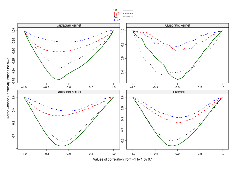
We can see that the total Kb-SIs are always greater than the first-order indices, as expected. While the Gaussian, Laplacian and L1L_{1} Kb-SIs give the same ranking of inputs, the quadratic Kb-SIs inversely identify X1X_{1} as the most important input for negative values of the correlation coefficient.

9 Conclusion

In this paper, we have proposed a new dependent measure of association between the model inputs and outputs and the associated statistical test of independence by making use of the total ANOVA functional (AF) of inputs and kernel methods. The proposed test statistic and dependent measures are i) well-suited for any output domain or object and models with non-independent variables, ii) much flexible for explicitly including specific moments of AFs, iii) able to distinguish two different distributions of AFs. Regarding the test statistics, we have provided generic kernels that guarantee the independence criterion between the outputs and the inputs. Most of characteristic kernels are equivalent kernels for the independence criterion. It comes out that convex and some concave kernels that guarantee the independence criterion lead to interesting dependent measures according to Rényi’ axioms.

In uncertainty quantification, the variance-based SA (Sobol’ indices; generalized sensitivity indices ([21, 22, 53, 48]) and dependent generalized sensitivity indices (dGSIs) ([38, 39])) and the Owen LpL^{p} measure are special cases of the proposed dependent measures by properly choosing the kernels. Moreover, it comes out that some kernels lead to the application of the maximum mean discrepancy and distance energy ([5, 6, 7, 8]). For the choice of kernels, we should prefer the importance-measure kernels that detect independence between inputs and outputs as effectively as possible, that is, account for the necessary and sufficient high-order moments such as the first and second-order moments for Gaussian-distributed AFs. For other distributions of AFs, the Laplacian, Gaussian and exponential kernels that account for all the moments of any distribution can be used since such kernels are importance-measure kernels for some values of their parameters. In general, Sobol’ indices and dGSIs are a first-order (resp. second-order) approximation of the proposed dependent measures associated with the Gaussian (resp. exponential) kernel.

The computations of AFs require evaluating conditional expectations of the model outputs given some inputs, and such evaluations may be time demanding to converge. In next future, it is interesting to investigate efficient methods for computing conditional expectations in high dimension. Gaussian process emulator ([54, 55]) of the models or new emulator based on the paper [49] or the Nadaraya-Watson kernel estimator for high-dimensional nonparametric regression ([56]) are going to be investigated.

Appendix A Proof of Lemma 1

We can see that the output f(𝐗)f(\mathbf{X}) is independent of 𝐗u\mathbf{X}_{u} implies

f(𝐗)=df(𝐗u,ru(𝐗u,𝐙))=:g(𝐗u,𝐙)=g(𝐙).f(\mathbf{X})\stackrel{{\scriptstyle d}}{{=}}f(\mathbf{X}_{u},r_{u}(\mathbf{X}_{u},\mathbf{Z}))=:g(\mathbf{X}_{u},\mathbf{Z})=g(\mathbf{Z})\,.

Therefore, we have gutot(𝐗u,𝐙)=g(𝐗u,𝐙)=𝔼𝐗u[g(𝐗u,𝐙)]=𝟎a.s.g^{tot}_{u}(\mathbf{X}_{u},\mathbf{Z})=g(\mathbf{X}_{u},\mathbf{Z})=\mathbb{E}_{\mathbf{X}_{u}}\left[g(\mathbf{X}_{u},\mathbf{Z})\right]=\mathbf{0}\,a.s..
Conversely, if gutot(𝐗u,𝐙)=𝟎g^{tot}_{u}(\mathbf{X}_{u},\mathbf{Z})=\mathbf{0}, the properties of conditional expectation show that there exists a function hh such that

g(𝐗u,𝐙)=𝔼𝐗u[g(𝐗u,𝐙)]=h(𝐙),g(\mathbf{X}_{u},\mathbf{Z})=\mathbb{E}_{\mathbf{X}_{u}}\left[g(\mathbf{X}_{u},\mathbf{Z})\right]=h(\mathbf{Z})\,,

which means that g(𝐗u,𝐙)g(\mathbf{X}_{u},\mathbf{Z}) is a function of 𝐙\mathbf{Z} only, and the result holds.

Appendix B Proof of Lemma 2

Bearing in mind Definition 4, we want to show that

𝔼[k(gutot(𝐗u,𝐙),gutot(𝐗u,𝐙))]k(𝟎,𝟎)=0,gutot(𝐗u,𝐙)=𝟎.\mathbb{E}\left[k\left(g^{tot}_{u}(\mathbf{X}_{u},\mathbf{Z}),\,g^{tot}_{u}(\mathbf{X}_{u}^{\prime},\mathbf{Z}^{\prime})\right)\right]-k(\mathbf{0},\mathbf{0})=0\,,\Longrightarrow\,g^{tot}_{u}(\mathbf{X}_{u},\mathbf{Z})=\mathbf{0}\,.

First, let us start with the kernel kk. Using the theorem of transfer, we can write

𝔼[k(gutot(𝐗u,𝐙),gutot(𝐗u,𝐙))]k(𝟎,𝟎)=𝒳2k(w,w)d(FTuFTuHH)(w,w),\mathbb{E}\left[k\left(g^{tot}_{u}(\mathbf{X}_{u},\mathbf{Z}),\,g^{tot}_{u}(\mathbf{X}_{u}^{\prime},\mathbf{Z}^{\prime})\right)\right]-k(\mathbf{0},\mathbf{0})=\int_{\mathcal{X}^{2}}k\left(w,w^{\prime}\right)\,d(F_{T_{u}}\otimes F_{T_{u}}-H\otimes H)(w,w^{\prime})\,,

with FTuF_{T_{u}} the CDF of gutot(𝐗u,𝐙)g^{tot}_{u}(\mathbf{X}_{u},\mathbf{Z}) and HH the CDF of δ𝟎\delta_{\mathbf{0}}. For a SPD kernel kk, when the above identity is zero, it implies that FTuFTu=HHF_{T_{u}}\otimes F_{T_{u}}=H\otimes H; FTu=HF_{T_{u}}=H and gutot(𝐗u,𝐙)=𝟎a.s.g^{tot}_{u}(\mathbf{X}_{u},\mathbf{Z})=\mathbf{0}\,a.s..
Second, we are going to use the criterion 𝔼𝐆F,𝐆F[k¯(𝐆,𝐆)]=0F=H\mathbb{E}_{\mathbf{G}\sim F,\mathbf{G}^{\prime}\sim F}\left[\bar{k}(\mathbf{G},\mathbf{G}^{\prime})\right]=0\Rightarrow F=H. Since k¯\bar{k} is centered at 𝟎\mathbf{0}, we have

𝔼[k¯(gutot(𝐗u,𝐙),gutot(𝐗u,𝐙))]k¯(𝟎,𝟎)=𝔼𝐆totFTu,𝐆totFTu[k¯(𝐆tot,𝐆tot)]=0,\mathbb{E}\left[\bar{k}\left(g^{tot}_{u}(\mathbf{X}_{u},\mathbf{Z}),\,g^{tot}_{u}(\mathbf{X}_{u}^{\prime},\mathbf{Z}^{\prime})\right)\right]-\bar{k}(\mathbf{0},\mathbf{0})=\mathbb{E}_{\mathbf{G}^{tot}\sim F_{T_{u}},\mathbf{G}^{tot^{\prime}}\sim F_{T_{u}}}\left[\bar{k}\left(\mathbf{G}^{tot},\,\mathbf{G}^{tot^{\prime}}\right)\right]=0\,,

which implies that FTu=HF_{T_{u}}=H.

Appendix C Proof of Lemma 3

For Point (i), we are going to use the first criterion of 𝒦E\mathcal{K}_{E} (see Equation (6)). We can write for all FF\in\mathcal{F}

𝔼𝐆F,𝐆F[k¯(𝐆,𝐆)]=𝔼𝐆F[k¯(,𝐆)]2=0𝔼𝐆F[k¯(,𝐆)]=0.\mathbb{E}_{\mathbf{G}\sim F,\mathbf{G}^{\prime}\sim F}\left[\bar{k}\left(\mathbf{G},\mathbf{G}^{\prime}\right)\right]=\left|\left|\mathbb{E}_{\mathbf{G}\sim F}\left[\bar{k}(\cdot,\mathbf{G})\right]\right|\right|_{\mathcal{H}}^{2}=0\Longleftrightarrow\mathbb{E}_{\mathbf{G}\sim F}\left[\bar{k}(\cdot,\mathbf{G})\right]=0\,.

Note that 𝔼𝐆F[k¯(,𝐆)]=0=𝔼WH[k¯(,W)]\mathbb{E}_{\mathbf{G}\sim F}\left[\bar{k}(\cdot,\mathbf{G})\right]=0=\mathbb{E}_{W\sim H}\left[\bar{k}(\cdot,W)\right] with HH the CDF of δ{𝟎}\delta_{\{\mathbf{0}\}}, and k¯\bar{k} is a characteristic kernel when kk is a characteristic one. Thus, Point (i) holds because 𝔼𝐆F[k¯(,𝐆)]=𝔼WH[k¯(,W)]\mathbb{E}_{\mathbf{G}\sim F}\left[\bar{k}(\cdot,\mathbf{G})\right]=\mathbb{E}_{W\sim H}\left[\bar{k}(\cdot,W)\right] implies F=HF=H.
For Point (ii), we are going to use the second criterion of 𝒦E\mathcal{K}_{E}. According to the Bochner Lemma and the Fubini theorem, we can write for independent vectors Y,ZY,Z

𝔼Yμ,Zμ[k(Y,Z)]\displaystyle\mathbb{E}_{Y\sim\mu,Z\sim\mu}\left[k(Y,Z)\right] =\displaystyle= 𝒳2k(𝐲,𝐳)𝑑μμ(𝐲,𝐳)\displaystyle\int_{\mathcal{X}^{2}}k(\mathbf{y},\mathbf{z})\,d\mu\otimes\mu(\mathbf{y},\mathbf{z})
=\displaystyle= 𝒳2nei𝐲T𝐰ei𝐳T𝐰𝑑μ(𝐲)𝑑μ(𝐳)𝑑Λ(𝐰)\displaystyle\int_{\mathcal{X}^{2}}\int_{\mathbb{R}^{n}}e^{-i\mathbf{y}^{T}\mathbf{w}}e^{i\mathbf{z}^{T}\mathbf{w}}\,d\mu(\mathbf{y})d\mu(\mathbf{z})d\Lambda(\mathbf{w})
=\displaystyle= n|𝒳ei𝐲T𝐰𝑑μ(𝐲)|2𝑑Λ(𝐰).\displaystyle\int_{\mathbb{R}^{n}}\left|\int_{\mathcal{X}}e^{-i\mathbf{y}^{T}\mathbf{w}}\,d\mu(\mathbf{y})\right|^{2}d\Lambda(\mathbf{w})\,.

Thus, 𝔼Yμ,Zμ[k(Y,Z)]=0\mathbb{E}_{Y\sim\mu,Z\sim\mu}\left[k(Y,Z)\right]=0 implies that ei𝐲T𝐰𝑑μ(𝐲)=0\int e^{-i\mathbf{y}^{T}\mathbf{w}}\,d\mu(\mathbf{y})=0 for all 𝐰Supp(Λ)=n\mathbf{w}\in Supp(\Lambda)=\mathbb{R}^{n}. For a class of finite and signed Borel measures of the form μ(A):=Ah(𝐲)𝑑𝐲\mu(A):=\int_{A}h(\mathbf{y})\,d\mathbf{y} with h:nh:\mathbb{R}^{n}\to\mathbb{R} a measurable function such as a difference of two probability densities, the function

h^(𝐰):=ei𝐲T𝐰𝑑μ(𝐲)=ei𝐲T𝐰h(𝐲)𝑑𝐲,𝐰Supp(Λ)=n,\widehat{h}(\mathbf{w}):=\int e^{-i\mathbf{y}^{T}\mathbf{w}}\,d\mu(\mathbf{y})=\int e^{-i\mathbf{y}^{T}\mathbf{w}}h(\mathbf{y})\,d\mathbf{y},\quad\forall\;\mathbf{w}\in Supp(\Lambda)=\mathbb{R}^{n}\,,

is the Fourier transform of h(𝐲)h(\mathbf{y}). As h^(𝐰)=0\widehat{h}(\mathbf{w})=0 for all 𝐰n\mathbf{w}\in\mathbb{R}^{n}, we then have h(𝐲)=0h(\mathbf{y})=0 bearing in mind the inverse Fourier transform. Point (ii) holds because μ=0\mu=0.

Appendix D Proof of Lemma 4

Let \mathcal{H} denote an Hilbert space induced by kk. Without loss of generality, we are going to show the results for q=1q=1.
First, using the convexity of J(f):=f2J(f):=\left|\left|f\right|\right|_{\mathcal{H}}^{2} with ff\in\mathcal{H}, we know that there exist a gradient of f2\left|\left|f\right|\right|_{\mathcal{H}}^{2} (i.e., J(f):=2f\nabla J(f):=2f) such that for all f0f_{0}\in\mathcal{H} ([52])

f2f022f0,ff0.\left|\left|f\right|\right|_{\mathcal{H}}^{2}-\left|\left|f_{0}\right|\right|_{\mathcal{H}}^{2}\geq\left<2f_{0},\,f-f_{0}\right>_{\mathcal{H}}\,.

Second, for 𝐆utot=gutot(𝐗u,𝐙)\mathbf{G}^{tot}_{u}\stackrel{{\scriptstyle}}{{=}}g^{tot}_{u}(\mathbf{X}_{u},\mathbf{Z}) and 𝐆ufo=gufo(𝐗u)\mathbf{G}^{fo}_{u}\stackrel{{\scriptstyle}}{{=}}g^{fo}_{u}(\mathbf{X}_{u}), we have (see Equation (4))

𝔼𝐙[gutot(𝐗u,𝐙)]=gufo(𝐗u).\mathbb{E}_{\mathbf{Z}}\left[g^{tot}_{u}(\mathbf{X}_{u},\mathbf{Z})\right]=g^{fo}_{u}(\mathbf{X}_{u})\,.

For Point (i), knowing that for the centered kernel k¯\bar{k},

𝒟k(FTu)=𝔼[k¯(𝐆utot,𝐆utot)]=𝔼[k(,𝐆utot)]k(,𝟎)2,\mathcal{D}_{k}(F_{T_{u}})=\mathbb{E}\left[\bar{k}\left(\mathbf{G}^{tot}_{u},\,\mathbf{G}^{tot^{\prime}}_{u}\right)\right]=\left|\left|\mathbb{E}\left[k\left(\cdot,\mathbf{G}^{tot}_{u}\right)\right]-k\left(\cdot,\mathbf{0}\right)\right|\right|_{\mathcal{H}}^{2}\,,

we can write (bearing in mind that k(𝟎,𝐲)=k(𝐲,𝟎)=ck(\mathbf{0},\mathbf{y}^{\prime})=k(\mathbf{y},\mathbf{0})=c)

𝒟k(FTu)𝒟k(Fu)=𝔼[k¯(𝐆utot,𝐆utot)]𝔼[k¯(𝐆ufo,𝐆ufo)]\displaystyle\mathcal{D}_{k}(F_{T_{u}})-\mathcal{D}_{k}(F_{u})=\mathbb{E}\left[\bar{k}\left(\mathbf{G}^{tot}_{u},\,\mathbf{G}^{tot^{\prime}}_{u}\right)\right]-\mathbb{E}\left[\bar{k}\left(\mathbf{G}^{fo}_{u},\,\mathbf{G}^{fo^{\prime}}_{u}\right)\right]
\displaystyle\geq 2𝔼[k(,𝐆ufo)]k(,𝟎),𝔼[k(,𝐆utot)]𝔼[k(,𝐆ufo)]\displaystyle 2\left<\mathbb{E}\left[k\left(\cdot,\mathbf{G}^{fo}_{u}\right)\right]-k\left(\cdot,\mathbf{0}\right),\;\mathbb{E}\left[k\left(\cdot,\mathbf{G}^{tot}_{u}\right)\right]-\mathbb{E}\left[k\left(\cdot,\mathbf{G}^{fo}_{u}\right)\right]\right>_{\mathcal{H}}
=\displaystyle= 2𝔼[k(𝐆utot,𝐆ufo)]2𝔼[k(𝐆ufo,𝐆ufo)]2𝔼[k(𝐆utot, 0)]+2𝔼[k(𝐆ufo, 0)]\displaystyle 2\mathbb{E}\left[k\left(\mathbf{G}^{tot}_{u},\,\mathbf{G}^{fo^{\prime}}_{u}\right)\right]-2\mathbb{E}\left[k\left(\mathbf{G}^{fo}_{u},\,\mathbf{G}^{fo^{\prime}}_{u}\right)\right]-2\mathbb{E}\left[k\left(\mathbf{G}^{tot}_{u},\,\mathbf{0}\right)\right]+2\mathbb{E}\left[k\left(\mathbf{G}^{fo}_{u},\,\mathbf{0}\right)\right]
=\displaystyle= 2𝔼[k(𝐆utot,𝐆ufo)]2𝔼[k(𝐆ufo,𝐆ufo)].\displaystyle 2\mathbb{E}\left[k\left(\mathbf{G}^{tot}_{u},\,\mathbf{G}^{fo^{\prime}}_{u}\right)\right]-2\mathbb{E}\left[k\left(\mathbf{G}^{fo}_{u},\,\mathbf{G}^{fo^{\prime}}_{u}\right)\right]\,.

Point (i) holds using the Jensen inequality and Equation (4).
For (ii), since 𝔼[𝐆utot]=𝔼[𝐆ufo]=𝟎\mathbb{E}[\mathbf{G}^{tot}_{u}]=\mathbb{E}[\mathbf{G}^{fo}_{u}]=\mathbf{0} and kk is convex, we can write 𝒟k(FTu)\mathcal{D}_{k}(F_{T_{u}}) without the absolute symbol thanks to Jensen’s theorem, that is,

𝒟k(FTu)=𝔼[k(𝐆utot,𝐆utot)]k(𝟎,𝟎)=𝔼[k(,𝐆utot)]2k(𝟎,𝟎).\mathcal{D}_{k}(F_{T_{u}})=\mathbb{E}\left[k\left(\mathbf{G}^{tot}_{u},\,\mathbf{G}^{tot^{\prime}}_{u}\right)\right]-k(\mathbf{0},\mathbf{0})=\left|\left|\mathbb{E}\left[k\left(\cdot,\mathbf{G}^{tot}_{u}\right)\right]\right|\right|_{\mathcal{H}}^{2}-k(\mathbf{0},\mathbf{0})\,.

Using the convexity of ||||2\left|\left|\cdot\right|\right|_{\mathcal{H}}^{2}, we can write

𝒟k(FTu)𝒟k(Fu)=𝔼[k(,𝐆utot)]2𝔼[k(,𝐆ufo)]2\displaystyle\mathcal{D}_{k}(F_{T_{u}})-\mathcal{D}_{k}(F_{u})=\left|\left|\mathbb{E}\left[k\left(\cdot,\mathbf{G}^{tot}_{u}\right)\right]\right|\right|_{\mathcal{H}}^{2}-\left|\left|\mathbb{E}\left[k\left(\cdot,\mathbf{G}^{fo}_{u}\right)\right]\right|\right|_{\mathcal{H}}^{2}
\displaystyle\geq 2𝔼[k(,𝐆ufo)],𝔼[k(,𝐆utot)]𝔼[k(,𝐆ufo)]\displaystyle 2\left<\mathbb{E}\left[k\left(\cdot,\mathbf{G}^{fo}_{u}\right)\right],\;\mathbb{E}\left[k\left(\cdot,\mathbf{G}^{tot}_{u}\right)\right]-\mathbb{E}\left[k\left(\cdot,\mathbf{G}^{fo}_{u}\right)\right]\right>_{\mathcal{H}}
=\displaystyle= 2𝔼[k(𝐆utot,𝐆ufo)]2𝔼[k(𝐆ufo,𝐆ufo)].\displaystyle 2\mathbb{E}\left[k\left(\mathbf{G}^{tot}_{u},\,\mathbf{G}^{fo^{\prime}}_{u}\right)\right]-2\mathbb{E}\left[k\left(\mathbf{G}^{fo}_{u},\,\mathbf{G}^{fo^{\prime}}_{u}\right)\right]\,.

Thus, Point (ii) holds using the Jensen inequality and Equation (4).
For Point (iii), as k(𝟎,𝟎)>0k(\mathbf{0},\mathbf{0})>0 and kk is concave, we have

𝒟k(FTu)=𝔼[k(𝐆utot,𝐆utot)]+k(𝟎,𝟎)=𝔼[k(,𝐆utot)]2+k(𝟎,𝟎),\mathcal{D}_{k}(F_{T_{u}})=-\mathbb{E}\left[k\left(\mathbf{G}^{tot}_{u},\,\mathbf{G}^{tot^{\prime}}_{u}\right)\right]+k(\mathbf{0},\mathbf{0})=-\left|\left|\mathbb{E}\left[k\left(\cdot,\mathbf{G}^{tot}_{u}\right)\right]\right|\right|_{\mathcal{H}}^{2}+k(\mathbf{0},\mathbf{0})\,,

and we can write

𝒟k(FTu)𝒟k(Fu)=𝔼[k(,𝐆ufo)]2𝔼[k(,𝐆utot)]2\displaystyle\mathcal{D}_{k}(F_{T_{u}})-\mathcal{D}_{k}(F_{u})=\left|\left|\mathbb{E}\left[k\left(\cdot,\mathbf{G}^{fo}_{u}\right)\right]\right|\right|_{\mathcal{H}}^{2}-\left|\left|\mathbb{E}\left[k\left(\cdot,\mathbf{G}^{tot}_{u}\right)\right]\right|\right|_{\mathcal{H}}^{2}
\displaystyle\geq 2𝔼[k(,𝐆utot)],𝔼[k(,𝐆ufo)]𝔼[k(,𝐆utot)]\displaystyle 2\left<\mathbb{E}\left[k\left(\cdot,\mathbf{G}^{tot}_{u}\right)\right],\;\mathbb{E}\left[k\left(\cdot,\mathbf{G}^{fo}_{u}\right)\right]-\mathbb{E}\left[k\left(\cdot,\mathbf{G}^{tot}_{u}\right)\right]\right>_{\mathcal{H}}
=\displaystyle= 2𝔼[k(𝐆ufo,𝐆utot)]2𝔼[k(𝐆utot,𝐆utot)].\displaystyle 2\mathbb{E}\left[k\left(\mathbf{G}^{fo}_{u},\,\mathbf{G}^{tot^{\prime}}_{u}\right)\right]-2\mathbb{E}\left[k\left(\mathbf{G}^{tot}_{u},\,\mathbf{G}^{tot^{\prime}}_{u}\right)\right]\,.

Using (4), Point (iii) holds by applying the Jensen inequality to k-k, which is convex.

Appendix E Proof of Theorem 1

Without loss of generality, we suppose that the outputs 𝐘:=g(𝐗w,𝐙w)\mathbf{Y}:=g(\mathbf{X}_{w},\mathbf{Z}_{\sim w}) is centered, that is, 𝔼[𝐘]=𝟎\mathbb{E}\left[\mathbf{Y}\right]=\mathbf{0}. Recall that AFs are also centered. Using wuw\subseteq u, we can write u=ww0u=w\cup w_{0} with w0uw_{0}\subseteq u and ww0=w\cap w_{0}=\emptyset. Thus, 𝐘:=g(𝐗w,𝐙w0,𝐙u)\mathbf{Y}:=g(\mathbf{X}_{w},\mathbf{Z}_{w_{0}},\mathbf{Z}_{\sim u}).
First, as gwfo(𝐗w)=𝔼𝐙w0𝐙u[g(𝐗w,𝐙w0,𝐙u)]g^{fo}_{w}(\mathbf{X}_{w})=\mathbb{E}_{\mathbf{Z}_{w_{0}}\mathbf{Z}_{\sim u}}\left[g(\mathbf{X}_{w},\mathbf{Z}_{w_{0}},\mathbf{Z}_{\sim u})\right], and it is known that (see [39]; Lemma 3) gufo(𝐗u)=dgufo(𝐗w,𝐙w0)=𝔼𝐙u[g(𝐗w,𝐙w0,𝐙u)]g^{fo}_{u}(\mathbf{X}_{u})\stackrel{{\scriptstyle d}}{{=}}g^{fo}_{u}(\mathbf{X}_{w},\mathbf{Z}_{w_{0}})=\mathbb{E}_{\mathbf{Z}_{\sim u}}\left[g(\mathbf{X}_{w},\mathbf{Z}_{w_{0}},\mathbf{Z}_{\sim u})\right], we can see that

gwfo(𝐗w)=d𝔼𝐙w0[gufo(𝐗w,𝐙w0)].g^{fo}_{w}(\mathbf{X}_{w})\stackrel{{\scriptstyle d}}{{=}}\mathbb{E}_{\mathbf{Z}_{w_{0}}}\left[g^{fo}_{u}(\mathbf{X}_{w},\mathbf{Z}_{w_{0}})\right]\,.

Second, for the convex kernel kk, the Jensen inequality allows for writting 𝒟k(Fw)\mathcal{D}_{k}(F_{w}) as

𝒟k(Fw)=𝔼[k(gwfo(𝐗w),gwfo(𝐗w))]k(𝟎,𝟎).\mathcal{D}_{k}(F_{w})=\mathbb{E}\left[k\left(g^{fo}_{w}(\mathbf{X}_{w}),\,g^{fo}_{w}(\mathbf{X}_{w}^{\prime})\right)\right]-k(\mathbf{0},\mathbf{0})\,.

Thus, the first result holds by applying the Jensen inequality, that is,

𝔼[k(gwfo(𝐗w),gwfo(𝐗w))]𝔼[k(gufo(𝐗u),gufo(𝐗u))].\mathbb{E}\left[k\left(g^{fo}_{w}(\mathbf{X}_{w}),\,g^{fo}_{w}(\mathbf{X}_{w}^{\prime})\right)\right]\leq\mathbb{E}\left[k\left(g^{fo}_{u}(\mathbf{X}_{u}),\,g^{fo}_{u}(\mathbf{X}_{u}^{\prime})\right)\right]\,.

For the second result, it comes out from the above equivalent in distribution that

gwtot(𝐗w,𝐙w0,𝐙u)=g(𝐗w,𝐙w0,𝐙u)𝔼𝐗w[g(𝐗w,𝐙w0,𝐙u)],g^{tot}_{w}(\mathbf{X}_{w},\mathbf{Z}_{w_{0}},\mathbf{Z}_{\sim u})=g(\mathbf{X}_{w},\mathbf{Z}_{w_{0}},\mathbf{Z}_{\sim u})-\mathbb{E}_{\mathbf{X}_{w}}\left[g(\mathbf{X}_{w},\mathbf{Z}_{w_{0}},\mathbf{Z}_{\sim u})\right]\,,
gutot(𝐗w,𝐙w0,𝐙u)=g(𝐗w,𝐙w0,𝐙u)𝔼𝐗w,𝐙w0[g(𝐗w,𝐙w0,𝐙u)],g^{tot}_{u}(\mathbf{X}_{w},\mathbf{Z}_{w_{0}},\mathbf{Z}_{\sim u})=g(\mathbf{X}_{w},\mathbf{Z}_{w_{0}},\mathbf{Z}_{\sim u})-\mathbb{E}_{\mathbf{X}_{w},\mathbf{Z}_{w_{0}}}\left[g(\mathbf{X}_{w},\mathbf{Z}_{w_{0}},\mathbf{Z}_{\sim u})\right]\,,

and we want to show that

𝔼[k(gwtot(𝐗w,𝐙w),gwtot(𝐗w,𝐙w))]𝔼[k(gutot(𝐗u,𝐙u),gutot(𝐗u,𝐙u))].\mathbb{E}\left[k\left(g^{tot}_{w}(\mathbf{X}_{w},\mathbf{Z}_{\sim w}),\,g^{tot}_{w}(\mathbf{X}_{w}^{\prime},\mathbf{Z}^{\prime}_{\sim w})\right)\right]\leq\mathbb{E}\left[k\left(g^{tot}_{u}(\mathbf{X}_{u},\mathbf{Z}_{\sim u}),\,g^{tot}_{u}(\mathbf{X}_{u}^{\prime},\mathbf{Z}^{\prime}_{\sim u})\right)\right]\,.

To that end, let 𝐕:=(𝐗w,𝐙w0,𝐙u)\mathbf{V}^{\prime}:=(\mathbf{X}_{w}^{\prime},\,\mathbf{Z}_{w_{0}}^{\prime},\,\mathbf{Z}_{\sim u}^{\prime}) be an i.i.d. copy of 𝐕:=(𝐗w,𝐙w0,𝐙u)\mathbf{V}:=(\mathbf{X}_{w},\mathbf{Z}_{w_{0}},\mathbf{Z}_{\sim u}); and consider the function h(𝐕,𝐕):=g(𝐗w,𝐙w0,𝐙u)g(𝐗w,𝐙w0,𝐙u)h(\mathbf{V},\mathbf{V}^{\prime}):=g(\mathbf{X}_{w},\mathbf{Z}_{w_{0}},\mathbf{Z}_{\sim u})-g(\mathbf{X}_{w}^{\prime},\mathbf{Z}_{w_{0}}^{\prime},\mathbf{Z}_{\sim u}^{\prime}). Since the three components of 𝐕\mathbf{V} (resp. 𝐕\mathbf{V}^{\prime}) are independent, we can write

𝔼[h(𝐕,𝐕)|𝐗w,δ𝟎(𝐙w0𝐙w0),δ𝟎(𝐙u𝐙u)]=gwtot(𝐗w,𝐙w0,𝐙u),\mathbb{E}\left[h(\mathbf{V},\mathbf{V}^{\prime})\,|\mathbf{X}_{w},\,\delta_{\mathbf{0}}(\mathbf{Z}_{w_{0}}^{\prime}-\mathbf{Z}_{w_{0}}),\,\delta_{\mathbf{0}}(\mathbf{Z}_{\sim u}^{\prime}-\mathbf{Z}_{\sim u})\right]=g^{tot}_{w}(\mathbf{X}_{w},\mathbf{Z}_{w_{0}},\mathbf{Z}_{\sim u})\,,
𝔼[h(𝐕,𝐕)|𝐗w,𝐙w0,δ𝟎(𝐙u𝐙u)]=gutot(𝐗w,𝐙w0,𝐙u).\mathbb{E}\left[h(\mathbf{V},\mathbf{V}^{\prime})\,|\mathbf{X}_{w},\mathbf{Z}_{w_{0}},\delta_{\mathbf{0}}(\mathbf{Z}_{\sim u}^{\prime}-\mathbf{Z}_{\sim u})\right]=g^{tot}_{u}(\mathbf{X}_{w},\mathbf{Z}_{w_{0}},\mathbf{Z}_{\sim u})\,.

Moreover, the properties of conditional expectation allow for writing

𝔼[gutot(𝐗w,𝐙w0,𝐙u)|𝐗w,δ𝟎(𝐙w0𝐙w0),δ𝟎(𝐙u𝐙u)]\displaystyle\mathbb{E}\left[g^{tot}_{u}(\mathbf{X}_{w},\mathbf{Z}_{w_{0}},\mathbf{Z}_{\sim u})\,|\mathbf{X}_{w},\,\delta_{\mathbf{0}}(\mathbf{Z}_{w_{0}}^{\prime}-\mathbf{Z}_{w_{0}}),\,\delta_{\mathbf{0}}(\mathbf{Z}_{\sim u}^{\prime}-\mathbf{Z}_{\sim u})\right]
=\displaystyle= 𝔼[𝔼[h(𝐕,𝐕)|𝐗w,𝐙w0,δ𝟎(𝐙u𝐙u)]|𝐗w,δ𝟎(𝐙w0𝐙w0),δ𝟎(𝐙u𝐙u)]\displaystyle\mathbb{E}\left[\mathbb{E}\left[h(\mathbf{V},\mathbf{V}^{\prime})\,|\mathbf{X}_{w},\mathbf{Z}_{w_{0}},\delta_{\mathbf{0}}(\mathbf{Z}_{\sim u}^{\prime}-\mathbf{Z}_{\sim u})\right]\,|\mathbf{X}_{w},\,\delta_{\mathbf{0}}(\mathbf{Z}_{w_{0}}^{\prime}-\mathbf{Z}_{w_{0}}),\,\delta_{\mathbf{0}}(\mathbf{Z}_{\sim u}^{\prime}-\mathbf{Z}_{\sim u})\right]
=\displaystyle= 𝔼[h(𝐕,𝐕)|𝐗w,δ𝟎(𝐙w0𝐙w0),δ𝟎(𝐙u𝐙u)]=gwtot(𝐗w,𝐙w0,𝐙u),\displaystyle\mathbb{E}\left[h(\mathbf{V},\mathbf{V}^{\prime})\,|\mathbf{X}_{w},\,\delta_{\mathbf{0}}(\mathbf{Z}_{w_{0}}^{\prime}-\mathbf{Z}_{w_{0}}),\,\delta_{\mathbf{0}}(\mathbf{Z}_{\sim u}^{\prime}-\mathbf{Z}_{\sim u})\right]=g^{tot}_{w}(\mathbf{X}_{w},\mathbf{Z}_{w_{0}},\mathbf{Z}_{\sim u})\,,

because the space of projection and the filtration associated with (𝐗w,𝐙w0,δ𝟎(𝐙u𝐙u))(\mathbf{X}_{w},\mathbf{Z}_{w_{0}},\,\delta_{\mathbf{0}}(\mathbf{Z}_{\sim u}^{\prime}-\mathbf{Z}_{\sim u})) contain those of (𝐗w,δ𝟎(𝐙w0𝐙w0),δ𝟎(𝐙u𝐙u))(\mathbf{X}_{w},\,\delta_{\mathbf{0}}(\mathbf{Z}_{w_{0}}^{\prime}-\mathbf{Z}_{w_{0}}),\,\delta_{\mathbf{0}}(\mathbf{Z}_{\sim u}^{\prime}-\mathbf{Z}_{\sim u})). The second result holds by applying the conditional Jensen inequality, as kk is convex.
Finally, the results for a concave kernel kk can be deduced from the above results. Indeed, we can see that k-k is convex and 𝒟k(Fw)\mathcal{D}_{k}(F_{w}) becomes

𝒟k(Fw)=𝔼[k(gwfo(𝐗w),gwfo(𝐗w))]+k(𝟎,𝟎).\mathcal{D}_{k}(F_{w})=\mathbb{E}\left[-k\left(g^{fo}_{w}(\mathbf{X}_{w}),\,g^{fo}_{w}(\mathbf{X}_{w}^{\prime})\right)\right]+k(\mathbf{0},\mathbf{0})\,.

Appendix F Proof of Corollary 1

It is sufficient to show the results for q=1q=1.
For Point (i), according to Theorem 1, we can write

0𝒟k(Fw)𝒟k(FTw)𝒟k(FTu),wu{1,,d}.0\leq\mathcal{D}_{k}(F_{w})\leq\mathcal{D}_{k}(F_{T_{w}})\leq\mathcal{D}_{k}(F_{T_{u}}),\quad\forall\,w\subseteq u\subseteq\{1,\ldots,d\}\,.

Thus, we have 0Sk(F)10\leq S_{k}(F)\leq 1 because F=FT{1,,d}F_{\bullet}=F_{T_{\{1,\ldots,d\}}}.
Point (ii) is obvious because k𝒦Ek\in\mathcal{K}_{E}, the set of kernels that guarantee the independence criterion.
The if part of Point (iii) is obvious. For the only if part, the equality 𝒟k(FTu)=𝒟k(F)\mathcal{D}_{k}(F_{T_{u}})=\mathcal{D}_{k}(F_{\bullet}) implies that

k(𝐲,𝐲)d(FTuFTuFF)(𝐲,𝐲)=0,\int k(\mathbf{y},\mathbf{y}^{\prime})\,d(F_{T_{u}}\otimes F_{T_{u}}-F_{\bullet}\otimes F_{\bullet})(\mathbf{y},\mathbf{y}^{\prime})=0\,,

which also implies that FTu=FF_{T_{u}}=F_{\bullet} for the second kind of kernels of 𝒦E\mathcal{K}_{E}.
Point (iv) holds for IMKs by definition.

Appendix G Proof of Theorem 2

Firstly, we have μ^(𝐙i)𝔼𝐗u[g(𝐗u,𝐙i)]0\widehat{\mu}(\mathbf{Z}_{i})-\mathbb{E}_{\mathbf{X}_{u}}\left[g(\mathbf{X}_{u},\mathbf{Z}_{i})\right]\to 0 when m1m_{1}\to\infty.
Knowing that 𝐆i,utot=g(𝐗i,u,𝐙i)𝔼𝐗u[g(𝐗u,𝐙i)]\mathbf{G}_{i,u}^{tot}=g(\mathbf{X}_{i,u},\mathbf{Z}_{i})-\mathbb{E}_{\mathbf{X}_{u}}\left[g(\mathbf{X}_{u},\mathbf{Z}_{i})\right] and 𝐆i,utot=g(𝐗i,u,𝐙i)𝔼𝐗u[g(𝐗u,𝐙i)]\mathbf{G}_{i,u}^{tot\,^{\prime}}=g(\mathbf{X}_{i,u}^{\prime},\mathbf{Z}_{i}^{\prime})-\mathbb{E}_{\mathbf{X}_{u}^{\prime}}\left[g(\mathbf{X}_{u}^{\prime},\mathbf{Z}_{i}^{\prime})\right], the Taylor expansion of kk about (𝐆i,utot,𝐆i,utot)\left(\mathbf{G}_{i,u}^{tot},\,\mathbf{G}_{i,u}^{tot\,^{\prime}}\right) yields

k(g(𝐗i,u,𝐙i)μ^(𝐙i),g(𝐗i,u,𝐙i)μ^(𝐙i))=k(𝐆i,utot,𝐆i,utot)\displaystyle k\left(g(\mathbf{X}_{i,u},\mathbf{Z}_{i})-\widehat{\mu}(\mathbf{Z}_{i}),\,g(\mathbf{X}_{i,u}^{\prime},\mathbf{Z}_{i}^{\prime})-\widehat{\mu}(\mathbf{Z}_{i}^{\prime})\right)=k\left(\mathbf{G}_{i,u}^{tot},\,\mathbf{G}_{i,u}^{tot\,^{\prime}}\right)
+Tk(𝐆i,utot,𝐆i,utot)[𝔼𝐗u[g(𝐗u,𝐙i)]μ^(𝐙i)𝔼𝐗u[g(𝐗u,𝐙i)]μ^(𝐙i)]+Rm1,\displaystyle+\nabla^{T}k\left(\mathbf{G}_{i,u}^{tot},\,\mathbf{G}_{i,u}^{tot\,^{\prime}}\right)\left[\begin{array}[]{c}\mathbb{E}_{\mathbf{X}_{u}}\left[g(\mathbf{X}_{u},\mathbf{Z}_{i})\right]-\widehat{\mu}(\mathbf{Z}_{i})\\ \mathbb{E}_{\mathbf{X}_{u}^{\prime}}\left[g(\mathbf{X}_{u}^{\prime},\mathbf{Z}_{i}^{\prime})\right]-\widehat{\mu}(\mathbf{Z}_{i}^{\prime})\end{array}\right]+R_{m_{1}}\,, (22)

where Rm1𝑃0R_{m_{1}}\xrightarrow{P}0 when m1m_{1}\to\leavevmode\nobreak\ \infty. Therefore, we can write

μktot^=1mi=1mk(𝐆i,utot,𝐆i,utot)\displaystyle\widehat{\mu_{k}^{tot}}=\frac{1}{m}\sum_{i=1}^{m}k\left(\mathbf{G}_{i,u}^{tot},\,\mathbf{G}_{i,u}^{tot\,^{\prime}}\right)
+1mi=1mTk(𝐆i,utot,𝐆i,utot)[𝔼𝐗u[g(𝐗u,𝐙i)]μ^(𝐙i)𝔼𝐗u[g(𝐗u,𝐙i)]μ^(𝐙i)]+Rm,m1,\displaystyle+\frac{1}{m}\sum_{i=1}^{m}\nabla^{T}k\left(\mathbf{G}_{i,u}^{tot},\,\mathbf{G}_{i,u}^{tot\,^{\prime}}\right)\left[\begin{array}[]{c}\mathbb{E}_{\mathbf{X}_{u}}\left[g(\mathbf{X}_{u},\mathbf{Z}_{i})\right]-\widehat{\mu}(\mathbf{Z}_{i})\\ \mathbb{E}_{\mathbf{X}_{u}^{\prime}}\left[g(\mathbf{X}_{u}^{\prime},\mathbf{Z}_{i}^{\prime})\right]-\widehat{\mu}(\mathbf{Z}_{i}^{\prime})\end{array}\right]+R_{m,m_{1}}\,, (25)

where Rm,m1𝑃0R_{m,m_{1}}\xrightarrow{P}0 when m1m_{1}\to\leavevmode\nobreak\ \infty. Since the second term of the above equation converge in probability toward 0, the LLN ensures that μktot^\widehat{\mu_{k}^{tot}} is a consistent estimator of μktot\mu_{k}^{tot}. thus, the first result of Point (i) holds.
Secondly, we obtain the second result of Point (i) by applying the central limit theorem (CLT) to the first term of the above equation, as the second term converge in probability toward 0.
The proof of Point (ii) is similar to the proof of Point (i). Indeed, using the Taylor expansion of k2k^{2}, we obtain the consistency of the second-order moment of kk. The Slutsky theorem ensures the consistency of the cross components and (μktot^)2\left(\widehat{\mu_{k}^{tot}}\right)^{2}.
Point (iii) is then obvious using Point (ii).
The proofs of Point (iv) is similar to those of Point (i).

Appendix H Proof of Corollary 2

First, the results about the consistency of the estimators are obtained by using Theorem 2 and the Slutsky theorem.
The numerators of Equations (15)-(16) are asymptotically distributed as Gaussian variable according to Theorem 2. To obtain the asymptotic distributions of the sensitivity indices, we first applied the Slutsky theorem, and second, we use the fact that m(STuk^𝔼[k(gutot,gutot)]k(𝟎,𝟎)1Mi=1Mk(g(𝐗i,u,𝐙i)μ^,g(𝐗i,u,𝐙i)μ^)k(𝟎,𝟎))\sqrt{m}\left(\widehat{S_{T_{u}}^{k}}-\frac{\mathbb{E}\left[k\left(g^{tot}_{u},\,g^{tot\,^{\prime}}_{u}\right)\right]-k(\mathbf{0},\mathbf{0})}{\frac{1}{M}\sum_{i=1}^{M}k\left(g(\mathbf{X}_{i,u},\mathbf{Z}_{i})-\widehat{\mu},\,g(\mathbf{X}_{i,u}^{\prime},\mathbf{Z}_{i}^{\prime})-\widehat{\mu}\right)-k(\mathbf{0},\mathbf{0})}\right) and m(STuk^STuk)\sqrt{m}\left(\widehat{S_{T_{u}}^{k}}-S_{T_{u}}^{k}\right) are asymptotically equivalent in probability under the technical condition m/M0m/M\to 0 (see [23] for more details).

Appendix I Proof of Lemma 5

For Point (i), the convexity of ψ\psi implies the existence of ψ\partial\psi such that

αψ(𝐲,𝐲)+αψ(𝐛,𝐲)αψ(𝐛,𝐲),𝐲𝐛,-\alpha\psi(\mathbf{y},\mathbf{y}^{\prime})+\alpha\psi(\mathbf{b},\mathbf{y}^{\prime})\leq\left<-\alpha\partial\psi(\mathbf{b},\mathbf{y}^{\prime}),\mathbf{y}-\mathbf{b}\right>\,,

which also implies (thanks to the Taylor expansion) that

eαψ(𝐲,𝐲)+αψ(𝐛,𝐲)eαψ(𝐛,𝐲),𝐲𝐛1+αψ(𝐛,𝐲),𝐲𝐛e^{-\alpha\psi(\mathbf{y},\mathbf{y}^{\prime})+\alpha\psi(\mathbf{b},\mathbf{y}^{\prime})}\leq e^{\left<-\alpha\partial\psi(\mathbf{b},\mathbf{y}^{\prime}),\mathbf{y}-\mathbf{b}\right>}\approx 1+\left<-\alpha\partial\psi(\mathbf{b},\mathbf{y}^{\prime}),\mathbf{y}-\mathbf{b}\right>\, (26)

under the condition (thanks to Cauchy-Schwartz)

|αψ(𝐛,𝐲),𝐲𝐛|αψ(𝐛,𝐲)2𝐲𝐛2ϵ𝐲,𝐛n.\left|\left<-\alpha\partial\psi(\mathbf{b},\mathbf{y}^{\prime}),\mathbf{y}-\mathbf{b}\right>\right|\leq\alpha\left|\left|\partial\psi(\mathbf{b},\mathbf{y}^{\prime})\right|\right|_{2}\,\left|\left|\mathbf{y}-\mathbf{b}\right|\right|_{2}\leq\epsilon\qquad\forall\,\mathbf{y}^{\prime},\mathbf{b}\in\mathbb{R}^{n}\,.

Equivalently, we can write αϵ𝐲𝐛2ψ(𝐛,𝐳)2;𝐲,𝐳,𝐛𝒳\alpha\leq\frac{\epsilon}{\left|\left|\mathbf{y}-\mathbf{b}\right|\right|_{2}\left|\left|\partial\psi(\mathbf{b},\mathbf{z})\right|\right|_{2}};\quad\forall\,\,\mathbf{y},\mathbf{z},\mathbf{b}\in\mathcal{X}. Equation (26) implies that kk is concave under the above condition. Indeed, we have

eαψ(𝐲,𝐲)+αψ(𝐛,𝐲)1\displaystyle e^{-\alpha\psi(\mathbf{y},\mathbf{y}^{\prime})+\alpha\psi(\mathbf{b},\mathbf{y}^{\prime})}-1 \displaystyle\leq αψ(𝐛,𝐲),𝐲𝐛\displaystyle\left<-\alpha\partial\psi(\mathbf{b},\mathbf{y}^{\prime}),\mathbf{y}-\mathbf{b}\right>
eαψ(𝐲,𝐲)eαψ(𝐛,𝐲)\displaystyle e^{-\alpha\psi(\mathbf{y},\mathbf{y}^{\prime})}-e^{-\alpha\psi(\mathbf{b},\mathbf{y}^{\prime})} \displaystyle\leq eαψ(𝐛,𝐲)αψ(𝐛,𝐲),𝐲𝐛\displaystyle e^{-\alpha\psi(\mathbf{b},\mathbf{y}^{\prime})}\left<-\alpha\partial\psi(\mathbf{b},\mathbf{y}^{\prime}),\mathbf{y}-\mathbf{b}\right>
k(𝐲,𝐲)+k(𝐛,𝐲)\displaystyle-k(\mathbf{y},\mathbf{y}^{\prime})+k(\mathbf{b},\mathbf{y}^{\prime}) \displaystyle\geq αψ(𝐛,𝐲)k(𝐛,𝐲),𝐲𝐛=k(𝐛,𝐲),𝐲𝐛,\displaystyle\left<\alpha\partial\psi(\mathbf{b},\mathbf{y}^{\prime})k(\mathbf{b},\mathbf{y}^{\prime}),\mathbf{y}-\mathbf{b}\right>=\left<\partial k(\mathbf{b},\mathbf{y}^{\prime}),\mathbf{y}-\mathbf{b}\right>\,,

with k(𝐛,𝐲):=αψ(𝐛,𝐲)k(𝐛,𝐲)\partial k(\mathbf{b},\mathbf{y}^{\prime}):=\alpha\partial\psi(\mathbf{b},\mathbf{y}^{\prime})k(\mathbf{b},\mathbf{y}^{\prime}) the subgradient of k-k. Thus, k-k is convex because kk is continuous ([52]).
For Point (ii), the gradient and the hessian of k(𝐲,𝐲)=eαψ(𝐲,𝐲)k(\mathbf{y},\mathbf{y}^{\prime})=e^{-\alpha\psi(\mathbf{y},\mathbf{y}^{\prime})} w.r.t. 𝐲\mathbf{y} are

k(𝐲,𝐲):=αψ(𝐲,𝐲)k(𝐲,𝐲),,\nabla k(\mathbf{y},\mathbf{y}^{\prime}):=-\alpha\nabla\psi(\mathbf{y},\mathbf{y}^{\prime})k(\mathbf{y},\mathbf{y}^{\prime}),\,,
Hk(𝐲,𝐲):=[αHψ(𝐲,𝐲)+α2ψ(𝐲,𝐲)Tψ(𝐲,𝐲)]k(𝐲,𝐲).H_{k}(\mathbf{y},\mathbf{y}^{\prime}):=\left[-\alpha H_{\psi}(\mathbf{y},\mathbf{y}^{\prime})+\alpha^{2}\nabla\psi(\mathbf{y},\mathbf{y}^{\prime})\nabla^{T}\psi(\mathbf{y},\mathbf{y}^{\prime})\right]k(\mathbf{y},\mathbf{y}^{\prime})\,.

Therefore, if we use E:=Hψ(𝐲,𝐲)+αψ(𝐲,𝐲)Tψ(𝐲,𝐲)E:=-H_{\psi}(\mathbf{y},\mathbf{y}^{\prime})+\alpha\nabla\psi(\mathbf{y},\mathbf{y}^{\prime})\nabla^{T}\psi(\mathbf{y},\mathbf{y}^{\prime}), then kk is concave when EE is negative definite. Thus, for all 𝐛𝒳\mathbf{b}\in\mathcal{X}, we can write

𝐛THψ(𝐲,𝐲)𝐛+α𝐛Tψ(𝐲,𝐲)Tψ(𝐲,𝐲)𝐛\displaystyle-\mathbf{b}^{T}H_{\psi}(\mathbf{y},\mathbf{y}^{\prime})\mathbf{b}+\alpha\mathbf{b}^{T}\nabla\psi(\mathbf{y},\mathbf{y}^{\prime})\nabla^{T}\psi(\mathbf{y},\mathbf{y}^{\prime})\mathbf{b} 0\displaystyle\leq 0
α(𝐛Tψ(𝐲,𝐲))2\displaystyle\alpha\left(\mathbf{b}^{T}\nabla\psi(\mathbf{y},\mathbf{y}^{\prime})\right)^{2} \displaystyle\leq 𝐛THψ(𝐲,𝐲)𝐛\displaystyle\mathbf{b}^{T}H_{\psi}(\mathbf{y},\mathbf{y}^{\prime})\mathbf{b}
α\displaystyle\alpha \displaystyle\leq 𝐛THψ(𝐲,𝐲)𝐛(𝐛Tψ(𝐲,𝐲))2.\displaystyle\frac{\mathbf{b}^{T}H_{\psi}(\mathbf{y},\mathbf{y}^{\prime})\mathbf{b}}{\left(\mathbf{b}^{T}\nabla\psi(\mathbf{y},\mathbf{y}^{\prime})\right)^{2}}\,.

Appendix J Proof of Corollary 4

Namely, we use u1(𝐲,𝐲,𝐲′′):=ϵ𝐲𝐲2ψ(𝐲,𝐲′′)2u_{1}(\mathbf{y},\mathbf{y}^{\prime},\mathbf{y}^{\prime\prime}):=\frac{\epsilon}{\left|\left|\mathbf{y}-\mathbf{y}^{\prime}\right|\right|_{2}\left|\left|\partial\psi(\mathbf{y}^{\prime},\mathbf{y}^{\prime\prime})\right|\right|_{2}} and u2(𝐲,𝐲,𝐲′′):=𝐲T′′Hψ(𝐲,𝐲)𝐲′′(ψ(𝐲,𝐲)T𝐲′′)2u_{2}(\mathbf{y},\mathbf{y}^{\prime},\mathbf{y}^{\prime\prime}):=\frac{\mathbf{y}^{{}^{\prime\prime}\,T}H_{\psi}(\mathbf{y},\mathbf{y}^{\prime})\mathbf{y}^{\prime\prime}}{\left(\nabla\psi(\mathbf{y},\mathbf{y}^{\prime})^{T}\,\mathbf{y}^{\prime\prime}\right)^{2}} for the upper bounds of α\alpha (see proof of Lemma 5). For the sequel of simplicity, we use u(𝐲,𝐲,𝐲′′)u(\mathbf{y},\mathbf{y}^{\prime},\mathbf{y}^{\prime\prime}) with 𝐲,𝐲,𝐲′′𝒳\mathbf{y},\mathbf{y}^{\prime},\mathbf{y}^{\prime\prime}\in\mathcal{X} for either u1(𝐲,𝐲,𝐲′′)u_{1}(\mathbf{y},\mathbf{y}^{\prime},\mathbf{y}^{\prime\prime}) or u2(𝐲,𝐲,𝐲′′)u_{2}(\mathbf{y},\mathbf{y}^{\prime},\mathbf{y}^{\prime\prime}).
As u(𝐘,𝐘,𝐘′′)u(\mathbf{Y},\mathbf{Y}^{\prime},\mathbf{Y}^{\prime\prime}) is random variable, we have (Markov’s inequality)

(u(𝐘,𝐘,𝐘′′)<α)=(1u(𝐘,𝐘,𝐘′′)>1α)α𝔼[1u(𝐘,𝐘,𝐘′′)]τ,\mathbb{P}\left(u(\mathbf{Y},\mathbf{Y}^{\prime},\mathbf{Y}^{\prime\prime})<\alpha\right)=\mathbb{P}\left(\frac{1}{u(\mathbf{Y},\mathbf{Y}^{\prime},\mathbf{Y}^{\prime\prime})}>\frac{1}{\alpha}\right)\leq\alpha\mathbb{E}\left[\frac{1}{u(\mathbf{Y},\mathbf{Y}^{\prime},\mathbf{Y}^{\prime\prime})}\right]\leq\tau\,,

which implies that ατ𝔼[1u(𝐘,𝐘,𝐘′′)]\alpha\leq\frac{\tau}{\mathbb{E}\left[\frac{1}{u(\mathbf{Y},\mathbf{Y}^{\prime},\mathbf{Y}^{\prime\prime})}\right]}.
Moreover, using Markov’s inequality we can write

1τ(u(𝐘,𝐘,𝐘′′)α)1α𝔼[u(𝐘,𝐘,𝐘′′)],1-\tau\leq\mathbb{P}\left(u(\mathbf{Y},\mathbf{Y}^{\prime},\mathbf{Y}^{\prime\prime})\geq\alpha\right)\leq\frac{1}{\alpha}\mathbb{E}\left[u(\mathbf{Y},\mathbf{Y}^{\prime},\mathbf{Y}^{\prime\prime})\right]\,,

which implies that α𝔼[u(𝐘,𝐘,𝐘′′)]1τ\alpha\leq\frac{\mathbb{E}\left[u(\mathbf{Y},\mathbf{Y}^{\prime},\mathbf{Y}^{\prime\prime})\right]}{1-\tau}.

References

  • [1] K. Pearson, On lines and planes of closest fit to systems of points in space, Philosophical Magazine 2 (1901) 559–572.
  • [2] H. Hotelling, Relations between two sets of variates, Vol. 28, 1936, pp. 321–377.
  • [3] I. Kojadinovic, M. Holmes, Tests of independence among continuous random vectors based on Cramr-von Mises functionals of the empirical copula process, Journal of Multivariate Analysis 100 (6) (2009) 1137–1154.
  • [4] Y. Escoufier, Le traitement des variables vectorielles, Biometrics 29 (1973) 751–760.
  • [5] K. M. Borgwardt, A. Gretton, M. J. Rasch, H.-P. Kriegel, B. Schölkopf, A. J. Smola, Integrating structured biological data by Kernel Maximum Mean Discrepancy, Bioinformatics 22 (14) (2006) 49–57.
  • [6] A. Gretton, K. Borgwardt, M. Rasch, B. Schölkopf, A. Smola, A kernel method for the two-sample-problem, in: B. Schölkopf, J. Platt, T. Hoffman (Eds.), Advances in Neural Information Processing Systems, Vol. 19, MIT Press, 2007.
  • [7] A. Gretton, K. M. Borgwardt, M. J. Rasch, B. Schölkopf, A. Smola, A kernel two-sample test, J. Mach. Learn. Res. 13 (2012) 723–773.
  • [8] M. L. Rizzo, G. J. Székely, Energy distance, WIREs Computational Statistics 8 (1) (2016) 27–38.
  • [9] A. Gretton, R. Herbrich, A. Smola, O. Bousquet, B. Schölkopf, Kernel methods for measuring independence, Journal of Machine Learning Research 6 (2005) 2075–2129.
  • [10] A. Gretton, O. Bousquet, A. Smola, B. Schölkopf, Measuring statistical dependence with hilbert-schmidt norms, in: International conference on algorithmic learning theory, Springer, 2005, pp. 63–77.
  • [11] D. Sejdinovic, B. Sriperumbudur, A. Gretton, K. Fukumizu, Equivalence of distance-based and RKHS-based statistics in hypothesis testing, The Annals of Statistics 41 (5) (2013) 2263–2291.
  • [12] A. Feuerverger, A consistent test for bivariate dependence, International Statistical Review / Revue Internationale de Statistique 61 (3) (1993) 419–433.
  • [13] G. J. Székely, M. L. Rizzo, N. K. Bakirov, Measuring and testing dependence by correlation of distances, The Annals of Statistics 35 (6) (2007) 2769–2794.
  • [14] S. Chatterjee, A new coefficient of correlation, Journal of the American Statistical Association (2020) 1–21.
  • [15] A. Renyi, On measures of dependence, Acta Mathematica Academiae Scientiarum Hungarica 10 (3-4) (1959) 441–451.
  • [16] B. K. Sriperumbudur, A. Gretton, K. Fukumizu, B. Schölkopf, G. R. Lanckriet, Hilbert space embeddings and metrics on probability measures, The Journal of Machine Learning Research 11 (2010) 1517–1561.
  • [17] J. Josse, S. Holmes, Measuring multivariate association and beyond, Statistics Surveys 10 (none) (2016) 132–167.
  • [18] E. de Rocquigny, N. Devictor, S. Tarantola (Eds.), Uncertainty in industrial practice, Wiley, 2008.
  • [19] I. M. Sobol, Sensitivity analysis for non-linear mathematical models, Mathematical Modelling and Computational Experiments 1 (1993) 407–414.
  • [20] A. Saltelli, K. Chan, E. Scott, Variance-Based Methods, Probability and Statistics, John Wiley and Sons, 2000.
  • [21] M. Lamboni, H. Monod, D. Makowski, Multivariate sensitivity analysis to measure global contribution of input factors in dynamic models, Reliability Engineering and System Safety 96 (2011) 450–459.
  • [22] F. Gamboa, A. Janon, T. Klein, A. Lagnoux, Sensitivity indices for multivariate outputs, Comptes Rendus Mathematique 351 (7) (2013) 307–310.
  • [23] M. Lamboni, Uncertainty quantification: a minimum variance unbiased (joint) estimator of the non-normalized Sobol’ indices, Statistical Papers (2018) –doi:https://doi.org/10.1007/s00362-018-1010-4.
  • [24] W. Hoeffding, A class of statistics with asymptotically normal distribution, Annals of Mathematical Statistics 19 (1948) 293–325.
  • [25] B. Efron, C. Stein, The jacknife estimate of variance, The Annals of Statistics 9 (1981) 586–596.
  • [26] A. Antoniadis, Analysis of variance on function spaces, Series Statistics 15 (1) (1984) 59–71.
  • [27] S. D. Veiga, Global sensitivity analysis with dependence measures, Journal of Statistical Computation and Simulation 85 (7) (2015) 1283–1305.
  • [28] S. Xiao, Z. Lu, P. Wang, Multivariate global sensitivity analysis for dynamic models based on energy distance, Structural and Multidisciplinary Optimization 57 (1) (2018) 279–291.
  • [29] E. Plischke, E. Borgonovo, Fighting the curse of sparsity: Probabilistic sensitivity measures from cumulative distribution functions, Risk Analysis 40 (12) (2020) 2639–2660.
  • [30] J. Barr, H. Rabitz, A generalized kernel method for global sensitivity analysis, SIAM/ASA Journal on Uncertainty Quantification 10 (1) (2022) 27–54.
  • [31] A. B. Owen, J. Dick, S. Chen, Higher order Sobol’ indices, Information and Inference: A Journal of the IMA 3 (1) (2014) 59–81.
  • [32] L. Song, A. Smola, A. Gretton, J. Bedo, K. Borgwardt, Feature selection via dependence maximization, Journal of Machine Learning Research 13 (5) (2012).
  • [33] S. Da Veiga, Kernel-based anova decomposition and shapley effects–application to global sensitivity analysis, arXiv preprint arXiv:2101.05487 (2021) –.
  • [34] A. Smola, A. Gretton, L. Song, B. Schölkopf, A hilbert space embedding for distributions, in: International Conference on Algorithmic Learning Theory, Springer, 2007, pp. 13–31.
  • [35] A. Gelman, Analysis of variance-why it is more important than ever, The Annals of Statistics 33 (1) (2005) 1 – 53.
  • [36] M. Lamboni, B. Iooss, A.-L. Popelin, F. Gamboa, Derivative-based global sensitivity measures: General links with Sobol’ indices and numerical tests, Mathematics and Computers in Simulation 87 (0) (2013) 45 – 54.
  • [37] M. Lamboni, Global sensitivity analysis: an efficient numerical method for approximating the total sensitivity index, International Journal for Uncertainty Quantification 6 (1) (2016) 1–17.
  • [38] M. Lamboni, S. Kucherenko, Multivariate sensitivity analysis and derivative-based global sensitivity measures with dependent variables, Reliability Engineering & System Safety 212 (2021) 107519.
  • [39] M. Lamboni, On dependent generalized sensitivity indices and asymptotic distributions, arXiv preprint arXiv2104.12938 (2021).
  • [40] M. Lamboni, Efficient dependency models: simulating dependent random variables, Mathematics and Computers in Simulation , submitted on 03/01/2021 (2021).
  • [41] M. Lamboni, Derivative-based integral equalities and inequality: A proxy-measure for sensitivity analysis, Mathematics and Computers in Simulation 179 (2021) 137 – 161.
  • [42] N. Aronszajn, Theory of reproducing kernels, Transactions of the American Mathematical Society 68 (1950) 337–404.
  • [43] B. Schölkopf, A. J. Smola, Learning with Kernels, MIT Press, Cambridge, MA, 2002.
  • [44] A. Berlinet, C. Thomas, T. A. Gnan, Reproducing Kernel Hilbert Space in probability and statistics, Kluwer Academic, 2004.
  • [45] K. Fukumizu, A. Gretton, X. Sun, B. Schölkopf, Kernel measures of conditional dependence, in: Proceedings of the 20th International Conference on Neural Information Processing Systems, NIPS’07, Curran Associates Inc., Red Hook, NY, USA, 2008, pp. 489–496.
  • [46] K. Fukumizu, A. Gretton, B. Schölkopf, B. K. Sriperumbudur, Characteristic kernels on groups and semigroups, in: D. Koller, D. Schuurmans, Y. Bengio, L. Bottou (Eds.), Advances in Neural Information Processing Systems, Vol. 21, Curran Associates, Inc., 2009.
  • [47] A. V. Skorohod, On a representation of random variables, Theory Probab. Appl 21 (3) (1976) 645–648.
  • [48] M. Lamboni, Derivative-based generalized sensitivity indices and Sobol’ indices, Mathematics and Computers in Simulation 170 (2020) 236 – 256.
  • [49] M. Lamboni, Weak derivative-based expansion of functions: Anova and some inequalities, Mathematics and Computers in Simulation 194 (2022) 691–718.
  • [50] K. Fukumizu, F. Bach, M. Jordan, Kernel dimensionality reduction for supervised learning, in: S. Thrun, L. Saul, B. Schölkopf (Eds.), Advances in Neural Information Processing Systems, Vol. 16, MIT Press, 2004.
  • [51] K. Fukumizu, A. Gretton, B. Schölkopf, B. K. Sriperumbudur, Characteristic kernels on groups and semigroups, in: D. Koller, D. Schuurmans, Y. Bengio, L. Bottou (Eds.), Advances in Neural Information Processing Systems, Vol. 21, Curran Associates, Inc., 2009.
  • [52] S. Boyd, L. Vandenberghe, Convex optimization, Cambridge university press, 2004.
  • [53] F. Gamboa, A. Janon, T. Klein, A. Lagnoux, Sensitivity analysis for multidimensional and functional outputs, Electron. J. Statist. 8 (1) (2014) 575–603.
  • [54] J. E. Oakley, A. O’Hagan, Probabilistic sensitivity analysis of complex models: a bayesian approach, Journal of the Royal Statistical Society: Series B (Statistical Methodology) 66 (3) (2004) 751–769.
  • [55] S. Conti, A. O’Hagan, Bayesian emulation of complex multi-output and dynamic computer models, Journal of Statistical Planning and Inference 140 (3) (2010) 640 – 651.
  • [56] D. Conn, G. Li, An oracle property of the Nadaraya -Watson kernel estimator for high-dimensional nonparametric regression, Scandinavian Journal of Statistics 46 (3) (2019) 735–764.