Kernel-based Optimally Weighted Conformal Prediction Intervals

Jonghyeok Lee H. Milton Stewart School of Industrial and Systems Engineering, Georgia Institute of Technology. Chen Xu H. Milton Stewart School of Industrial and Systems Engineering, Georgia Institute of Technology. Yao Xie Correspondence: yao.xie@isye.gatech.edu H. Milton Stewart School of Industrial and Systems Engineering, Georgia Institute of Technology.

Abstract

Conformal prediction has been a popular distribution-free framework for uncertainty quantification. In this work, we present a novel conformal prediction method for time-series, which we call Kernel-based Optimally Weighted Conformal Prediction Intervals (KOWCPI). Specifically, KOWCPI adapts the classic Reweighted Nadaraya-Watson (RNW) estimator for quantile regression on dependent data and learns optimal data-adaptive weights. Theoretically, we tackle the challenge of establishing a conditional coverage guarantee for non-exchangeable data under strong mixing conditions on the non-conformity scores. We demonstrate the superior performance of KOWCPI on real time-series against state-of-the-art methods, where KOWCPI achieves narrower confidence intervals without losing coverage.

1 Introduction

Conformal prediction, originated in Vovk et al. (1999, 2005), offers a robust framework explicitly designed for reliable and distribution-free uncertainty quantification. Conformal prediction has become increasingly recognized and adopted within the domains of machine learning and statistics (Lei et al., 2013; Lei and Wasserman, 2014; Kim et al., 2020; Angelopoulos and Bates, 2023). Assuming nothing beyond the exchangeability of data, conformal prediction excels in generating valid prediction sets under any given significance level, irrespective of the underlying data distribution and model assumptions. This capability makes it particularly valuable for uncertainty quantification in settings characterized by diverse and complex models.

Going beyond the exchangeability assumption has been a research challenge, particularly as many real-world datasets (such as time-series data) are inherently non-exchangeable. Tibshirani et al. (2019) addresses situations where a feature distribution shifts between training and test data and restores valid coverage through weighted quantiles based on the likelihood ratio of the distributions. More recently, Barber et al. (2023) bounds the coverage gap using the total variation distance between training and test data eights and minimizes this gap using pre-specified data-independent weights. However, it remains open to how to appropriately optimize the weights.

To advance conformal prediction for time series, we extend the prior sequential predictive approach (Xu and Xie, 2023a, b) by incorporating nonparametric kernel regression into the quantile regression method on non-conformity scores. A key challenge of adapting this method to time-series data lies in selecting optimal weights to accommodate the dependent structure of the data. To ensure valid coverage of prediction sets, it is crucial to select weights inside the quantile estimator so that it closely approximates the true quantile of non-conformity scores.

In this paper, we introduce KOWCPI, which utilizes the Reweighted Nadaraya-Watson estimator (Hall et al., 1999) to facilitate the selection of data-dependant optimal weights. This approach anticipates that adaptive weights will enhance the robustness of uncertainty quantification, particularly when the assumption of exchangeability is compromised. Our method also addresses the weight selection issue in the weighted quantile method presented by Barber et al. (2023), as KOWCPI allows for the calculation of weights in a data-driven manner without prior knowledge about the data.

In summary, our main contributions are:

•

We propose KOWCPI, a sequential time-series conformal prediction method that performs nonparametric kernel quantile regression on non-conformity scores. In particular, KOWCPI learns optimal data-driven weights used in the conditional quantiles.
•

We prove the asymptotic conditional coverage guarantee of KOWCPI based on the classical theory of nonparametric regression. We further obtain the marginal coverage gap of KOWCPI using the general result for the weights on quantile for non-exchangeable data.
•

We demonstrate the effectiveness of KOWCPI on real time-series data against state-of-the-art baselines. Specifically, KOWCPI can achieve the narrowest width of prediction intervals without losing marginal and approximate conditional (i.e., rolling) coverage empirically.

1.1 Literature

RNW quantile regression

In Hall et al. (1999), the Reweighted Nadaraya-Watson (RNW, often referred to as Weighted or Adjusted Nadaraya-Watson) estimator was suggested as a method to estimate the conditional distribution function from time-series data. This estimator extends the renowned Nadaraya-Watson estimator (Nadaraya, 1964; Watson, 1964) by introducing an additional adjustment to the weights, thus combining the favorable bias properties of the local linear estimator with the benefit of being a distribution function by itself like the original Nadaraya-Watson estimator (Hall et al., 1999; Yu and Jones, 1998). The theory of the regression quantile with the RNW estimator has been further developed by Cai (2002). Furthermore, Cai (2002) and Salha (2006) demonstrated that the RNW estimator is consistent under strongly mixing conditions, which are commonly observed in time-series data. In this work, we adaptively utilize the RNW estimator within the conformal prediction framework to construct sequential prediction intervals for time-series data, leveraging its data-driven weights for quantile estimation and the weighted conformal approach.

Conformal prediction with weighted quantiles

Approaches using quantile regression instead of empirical quantiles in conformal prediction have been widespread (Romano et al., 2019; Kivaranovic et al., 2020; Gibbs et al., 2023). These methods utilize various quantile regression techniques to construct conformal prediction intervals, and the convergence to the oracle prediction width can be shown under the consistency of the quantile regression function (Sesia and Candès, 2020). Another recent work by Guan (2023) uses kernel weighting based on the distance between the test point and data to perform localized conformal prediction, which further discusses the selection of kernels and bandwidths. Recent work in this direction of utilizing the weighted quantiles, including Lee et al. (2023); Angelopoulos et al. (2023), continues to be vibrant. As we will discuss later, our approach leverages techniques in classical non-parametric statistics when constructing the weights.

Time-series conformal prediction

There is a growing body of research on time-series conformal prediction (Xu and Xie, 2021b; Gibbs and Candès, 2021). Various applications include financial markets (Gibbs and Candès, 2021), anomaly detection (Xu and Xie, 2021a), and geological classification (Xu and Xie, 2022). In particular, Gibbs and Candès (2021, 2022) sequentially construct prediction intervals by updating the significance level $\alpha$ based on the mis-coverage rate. This approach has become a major methodology for handling non-exchangeable data, leading to several subsequent developments (Feldman et al., 2022; Auer et al., 2023; Bhatnagar et al., 2023; Zaffran et al., 2022). On the other hand, Xu and Xie (2023b); Xu et al. (2024) take a slightly different approach by conducting sequential quantile regression using non-conformity scores. Our study aims to integrate non-parametric kernel estimation for sequential quantile regression, addressing the weight selection issues identified by Barber et al. (2023). Additionally, our research aligns with Guan (2023), particularly in utilizing a dissimilarity measure between the test point and the past data.

2 Problem Setup

We begin by assuming that the observations of the random sequence $(X_{t},Y_{t})\in\mathbb{R}^{d}\times\mathbb{R}$ , $t=1,2,\ldots$ are obtained sequentially. Notably, $X_{t}$ may represent exogenous variables that aid in predicting $Y_{t}$ , the historical values of $Y_{t}$ itself, or a combination of both. (In Appendix A, we expand our discussion to include cases where the response $Y_{t}$ is multivariate.) A key aspect of our setup is that the data are non-exchangeable and exhibit dependencies, which are typical in time-series data where temporal or sequential dependencies influence predictive dynamics.

Suppose we are given a pre-specified point predictor $\hat{f}:\mathbb{R}^{d}\to\mathbb{R}$ trained on a separate dataset or on past data. This predictor $\hat{f}$ maps a feature variable in $\mathbb{R}^{d}$ to a scalar point prediction for $Y_{t}$ . Given a user-specified significance level $\alpha\in(0,1)$ , we use the initial $T$ observations to construct prediction intervals $\widehat{C}_{t-1}^{\alpha}(X_{t})$ for $Y_{t}$ in a sequential manner from $t=T+1$ onwards.

Two key types of coverage targeted by prediction intervals are marginal coverage and conditional coverage. Marginal coverage is defined as

\mathbb{P}(Y_{t}\in\widehat{C}_{t-1}^{\alpha}(X_{t}))\geq 1-\alpha,

(1)

which ensures that the true value $Y_{t}$ falls within the interval $\widehat{C}_{t-1}^{\alpha}(X_{t})$ at least $100(1-\alpha)\%$ of the time, averaged over all instances. On the other hand, conditional coverage is defined as

\mathbb{P}(Y_{t}\in\widehat{C}_{t-1}^{\alpha}(X_{t})\mid X_{t})\geq 1-\alpha,

(2)

which is a stronger guarantee ensuring that given each value of predictor $X_{t}$ , the true value $Y_{t}$ falls within the interval $\widehat{C}_{t-1}^{\alpha}(X_{t})$ at least $100(1-\alpha)\%$ of the time.

3 Method

In this section, we introduce our proposed method, KOWCPI (Kernel-based Optimally Weighted Conformal Prediction Intervals), which embodies our approach to enhancing prediction accuracy and robustness in the face of time-series data. We delve into the methodology and algorithm of KOWCPI in-depth, highlighting how the Reweighted Nadaraya-Watson (RNW) estimator integrates with our predictive framework.

Consider prediction for a univariate time series, $Y_{1},Y_{2},\ldots$ . We have predictors $X_{t}$ given to us at time $t$ , $t=1,2,\ldots$ , which can depend on the past observations $(Y_{t-1},Y_{t-2},\ldots)$ , and possibly other exogeneous time series $Z_{t}$ . Given a pre-trained algorithm $\hat{f}$ , we also have a sequence of non-conformity scores indicating the accuracy of the prediction:

\hat{\varepsilon}_{t}=Y_{t}-\hat{f}(X_{t}),\quad t=1,2,\ldots.

We denote the collection of the past $T$ non-conformity scores at time $t>T$ as

\mathcal{E}_{t}=(\hat{\varepsilon}_{t-1},\ldots,\hat{\varepsilon}_{t-T}),

We construct the prediction interval $\widehat{C}_{t-1}^{\alpha}(X_{t})$ with significance level $\alpha$ at time $t>T$ as follows:

\displaystyle\begin{split}\widehat{C}_{t-1}^{\alpha}(X_{t})&=[\hat{f}(X_{t})+\hat{q}_{\beta^{*}}(\mathcal{E}_{t}),\hat{f}(X_{t})+\hat{q}_{1-\alpha+\beta^{*}}(\mathcal{E}_{t})],\\ \beta^{*}&=\mathop{\rm argmin}_{\beta\in[0,\alpha]}\left(\hat{q}_{1-\alpha+\beta}(\mathcal{E}_{t})-\hat{q}_{\beta}(\mathcal{E}_{t})\right).\end{split}

(3)

Here, $\hat{q}_{\beta}$ is a quantile regression algorithm that returns an estimate of the $\beta$ -quantile of the residuals, which we will explain through this section. We consider asymmetrical confidence intervals to ensure the tightest possible coverage.

3.1 Reweighted Nadaraya-Watson estimator

The Reweighted Nadaraya-Watson (RNW) estimator is a general and popular method for quantile regression. Observe $(\tilde{X}_{i},\tilde{Y}_{i})$ , $i=1,\ldots,n$ , where $\tilde{Y}_{i}\in\mathbb{R}$ , and the predictors $\tilde{X}_{i}$ can be $p$ -dimensional. The goal is to predict the quantile $\mathbb{P}(\tilde{Y}\leq b|\tilde{X})$ , $b\in\mathbb{R}$ , given a test point $\tilde{X}$ using training samples. The RNW estimator introduces adjustment weights on the predictors to ensure consistent estimation. We define the probability-like adjustment weights $p_{i}(\tilde{X})$ , $i=1,\ldots,n$ , by maximizing the empirical log-likelihood $\sum_{i=1}^{n}\log p_{i}(\tilde{X})$ , subject to $p_{i}(\tilde{X})\geq 0$ , and

		$\displaystyle\sum_{i=1}^{n}p_{i}(\tilde{X})=1,$		(4)
		$\displaystyle\sum_{i=1}^{n}p_{i}(\tilde{X})(\tilde{X}_{i}-\tilde{X})K_{h}(\tilde{X}_{i}-\tilde{X})=0.$		(5)

The RNW estimate of the conditional CDF $\mathbb{P}(\tilde{Y}\leq b|\tilde{X})$ is defined as follows:

\displaystyle\widehat{F}(b|\tilde{X})=\sum_{i=1}^{n}\widehat{W}_{i}(\tilde{X})\mathds{1}(\tilde{Y}_{i}\leq b),

(6)

where the weights are given by

\widehat{W}_{i}(\tilde{X})=\frac{p_{i}(\tilde{X})K_{h}(\tilde{X}_{i}-\tilde{X})}{\sum_{i=1}^{n}p_{i}(\tilde{X})K_{h}(\tilde{X}_{i}-\tilde{X})},\quad i=1,\ldots,n.

(7)

Here, the kernel $K\colon\mathbb{R}^{p}\to\mathbb{R}$ is a kernel function, and $K_{h}(\mathbf{u})=h^{-p}K(h^{-1}\mathbf{u})$ for $\mathbf{u}\in\mathbb{R}^{p}$ . Any reasonable choice of kernel function is possible; however, to ensure the validity of our theoretical results discussed in Section 4, the kernel should be nonnegative, bounded, continuous, and possess compact support. An example is $K(u)=k(\left\|u\right\|)$ , where $k:\mathbb{R}\to\mathbb{R}$ is the Epanechnikov kernel.

The computation of $p_{i}(\tilde{X})$ reduces to a simple one-dimensional convex minimization problem:

Lemma 3.1 ((Hall et al., 1999; Cai, 2001)).

The adjustment weights $p_{i}(\tilde{X})$ , $i=1,\ldots,n$ , for the RNW estimator are given as

p_{i}(\tilde{X})=\frac{1}{n}\left[1+\lambda([\tilde{X}_{i}]_{1}-[\tilde{X}]_{1})K_{h}(\tilde{X}_{i}-\tilde{X})\right]^{-1},

(8)

where $[X]_{1}$ denotes the first element of a vector $X$ , and $\lambda\in\mathbb{R}$ is the minimizer of:

L(\lambda;\tilde{X})=-\sum_{i=1}^{n}\log\{1+\lambda([\tilde{X}_{i}]_{1}-[\tilde{X}]_{1})K_{h}(\tilde{X}_{i}-\tilde{X})\}.

(9)

Lemma 3.1 is a starting point for the proof of the asymptotic conditional coverage property of our algorithm later on.

3.2 RNW for conformal prediction

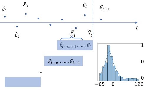
Refer to caption — Figure 1: Illustration of Kernel-based Optimally Weighted Conformal Prediction Intervals (KOWCPI).

To perform the quantile regression for prediction interval construction at time $t=T+1$ , we use a sliding window approach, breaking the past $T$ residuals $\mathcal{E}_{T+1}=(\hat{\varepsilon}_{T},\ldots\hat{\varepsilon}_{1})$ into $n\coloneqq(T-w)$ overlapping segments of length $w$ . We construct the predictors and responses to fit the RNW estimator as follows:

\tilde{Y}_{i}=\hat{\varepsilon}_{i+w},\quad\tilde{X}_{i}=(\hat{\varepsilon}_{i+w-1},\ldots,\hat{\varepsilon}_{i}),\quad i=1,\ldots,n.

With RNW estimator $\widehat{F}$ fitted on $((\tilde{X}_{i},\tilde{Y}_{i}))_{i=1}^{n}$ , the conditional $\beta$ -quantile estimator $\widehat{Q}_{\beta}$ is defined as

\widehat{Q}_{\beta}(\tilde{X})\coloneqq\inf\{\tilde{y}\in\mathbb{R}\colon\widehat{F}(\tilde{y}|\tilde{X})\geq\beta\}.

(10)

After time $t=T+1$ , we update $\mathcal{E}_{t}$ by removing the oldest residual and adding the newest one, then repeat the process (see Algorithm 1). In Section 4, we prove that due to the consistency of $\widehat{Q}_{\beta}$ , KOWCPI achieves asymptotic conditional coverage despite the significant temporal dependence introduced by using overlapping segments of residuals.

Algorithm 1 Kernel-based Optimally Weighted Conformal Prediction Intervals (KOWCPI)

0: Sequentially obtained data

(X_{t},Y_{t})

t=1,2,\ldots

, pre-trained point predictor

\hat{f}

, Target significance level

\alpha\in(0,1)

1: Obtain prediction residuals

\hat{\varepsilon}_{t}=Y_{t}-\hat{f}(X_{t})

t=1,\ldots,T

2: for

t=T+1,\ldots

3: Update

\mathcal{E}_{t}=(\hat{\varepsilon}_{t-1},\ldots,\hat{\varepsilon}_{t-T})

4: Break

\mathcal{E}_{t}

into overlapping segments

\tilde{X}_{i}=(\hat{\varepsilon}_{t-T+i+w-2},\ldots,\hat{\varepsilon}_{t-T+i-1})

i=1,\ldots,n+1

5: Obtain

\lambda

that minimizes

L(\cdot;\tilde{X}_{n+1})

in (9).

6: Obtain the adjustment weights

p_{i}(\tilde{X}_{n+1}),i=1,\ldots,n

, and thus final weights

\hat{W}_{i}(\tilde{X}_{n+1})

7: With

\tilde{Y}_{i}=\hat{\varepsilon}_{t-T+i+w-1}

i=1,\ldots,n

, derive the quantile estimator

\widehat{Q}_{\beta}(\tilde{X}_{n+1})

for

\beta\in[0,\alpha]

8: Obtain

\beta^{*}=\mathop{\rm argmin}_{\beta\in[0,\alpha]}\widehat{Q}_{1-\alpha+\beta}(\tilde{X}_{n+1})-\widehat{Q}_{\beta}(\tilde{X}_{n+1})

9: Return

\widehat{C}_{t-1}^{\alpha}(X_{t})=[\hat{f}(X_{t})+\widehat{Q}_{\beta^{*}}(\tilde{X}_{n+1}),~{}\hat{f}(X_{t})+\widehat{Q}_{1-\alpha+\beta^{*}}(\tilde{X}_{n+1})]

10: Obtain a new residual

\hat{\varepsilon}_{t}

11: end for

Bandwidth selection

While it is theoretically possible to calculate the optimal bandwidth that minimizes the asymptotic mean-squared error, this requires additional derivative estimation, which significantly complicates the problem. Consequently, similar to general non-parametric models, one can use cross-validation to select the bandwidth. However, cross-validation can be computationally burdensome and may deteriorate under dependent data (Fan et al., 1995). Therefore, we adapt the non-parametric AIC (Cai and Tiwari, 2000), used for bandwidth selection in local linear estimators. This method is applicable because the RNW estimator belongs to the class of linear smoother (Cai, 2002). We choose the bandwidth $h$ that minimizes

{\rm AIC}_{C}(h)\coloneqq\log({\rm RSS})+\frac{n+\mbox{tr}(SS^{\top})}{n-(\mbox{tr}(SS^{\top})+2)},

(11)

where ${\rm RSS}$ is the residual sum of squares, and $S$ is a linear smoothing operator (Hastie, 1990), with the $(i,j)$ -th element given by $S_{ij}=\widehat{W}_{j}(\tilde{X}_{i}).$

Window length selection

To select the window length $w$ , cross-validation can be employed. One approach is to use a weighted sum of the average under-coverage rate and the average width obtained for a given $w$ as the criterion. Another approach could involve choosing $w$ with the smallest average width that achieves a target coverage in the validation set. In experiments, we observed that the performance is less sensitive to the choice of $w$ across a broader range compared to the bandwidth $h$ , although the selection of $h$ and $w$ interactively affects the performance.

4 Theory

In this section, we introduce the theoretical properties of the RNW estimator, a quantile regression method we use, and demonstrate in Theorem 4.9 that our KOWCPI asymptotically displays conditional coverage under the strong mixing of residuals. It turns out that the asymptotic conditional coverage gap can be derived from known results in the context of kernel quantile regression.

4.1 Marginal coverage

We begin by bounding the marginal coverage gap of the KOWCPI method. The following result shows the coverage gap using our weights, compared with the oracle weights; the results are established using a similar strategy as in (Tibshirani et al., 2019, Lemma 3):

Proposition 4.1 (Non-asymptotic marginal coverage gap).

Denote by $\mathcal{P}$ the joint density of $(\tilde{Y}_{1},\ldots,\tilde{Y}_{n+1})$ . Then, we have

\displaystyle\begin{split}&\left|\mathbb{P}\left(Y_{T+1}\in\widehat{C}_{T}^{\alpha}(X_{T+1})\right)-(1-\alpha)\right|\\ &\leq\frac{1}{2}\left(\mathbb{E}\left\|(W^{*})_{1:n}-\widehat{W}\right\|_{1}+\mathbb{E}W^{*}_{n+1}\right)+2\mathbb{E}\Delta(\tilde{X}_{n+1})\end{split}

(12)

where $\Delta(\tilde{X}_{n+1})$ is the discrete gap defined in (17), and $W^{*}$ is the vector of oracle weights with each entry is defined as

W_{i}^{*}:=\frac{\sum_{\sigma:\sigma(n+1)=i}\mathcal{P}(\tilde{Y}_{\sigma(1)},\ldots,\tilde{Y}_{\sigma(n+1)})}{\sum_{\sigma}\mathcal{P}(\tilde{Y}_{\sigma(1)},\ldots,\tilde{Y}_{\sigma(n+1)})},\quad i=1,\ldots,{n+1},\quad\mbox{(oracle weights)}

(13)

and $\sigma$ is a permutation on $\{1,\ldots,n+1\}$ .

The implication of Proposition 4.1 is that

•

The “under-coverage” depends on the $\ell_{1}$ -distance between the learned optimal weights and oracle-optimal weights (that depends on the true joint distribution of data).
•

Note that the oracle weights $W_{t}^{*}$ cannot be evaluated, because in principle, it requires considering the $(n+1)!$ possible shuffled observed residuals and their joint distributions.
•

The form of the oracle weights $W_{i}^{*}$ from (13) offers an intuitive basis for algorithm development: we can practically estimate the weights through quantile regression, utilizing previously observed non-conformity scores.

4.2 Conditional coverage

In this section, we derive the asymptotic conditional coverage property of KOWCPI. For this, we introduce the assumptions necessary for the consistency of the RNW estimator. To account for the dependency in the data, we assume the strong mixing of the residual process.

A stationary stochastic process $\{V_{t}\}_{t=-\infty}^{\infty}$ on a probability space with a probability measure $\mathbb{P}$ is said to be strongly mixing ( $\alpha$ -mixing) if a mixing coefficient $\alpha(\tau)$ defined as

\alpha(\tau)=\sup_{A\in\mathfrak{M}_{-\infty}^{0},B\in\mathfrak{M}_{\tau}^{\infty}}\left|\mathbb{P}(A\cap B)-\mathbb{P}(A)\mathbb{P}(B)\right|

satisfies $\alpha(\tau)\to 0$ as $\tau\to\infty$ , where $\mathfrak{M}_{s}^{t}$ , $-\infty\leq s\leq t\leq\infty$ , denotes a $\sigma$ -algebra generated by $\{V_{s},V_{s+1},\ldots,V_{t}\}$ . The mixing coefficient $\alpha(\tau)$ quantifies the asymptotic independence between the past and future of the sequence $\{V_{t}\}_{t=-\infty}^{\infty}$ .

Assumption 4.2 (Mixing of the process).

The stationary process $(V_{i}=(\tilde{X}_{i},\tilde{Y}_{i}))_{i=1}^{\infty}$ is strongly mixing with the mixing coefficient $\alpha(\tau)=\mathcal{O}(\tau^{-(2+\delta)})$ for some $\delta>0$ .

Due to stationarity, the conditional CDF of the realized residual does not depend on the index $i$ ; thus, denote

F(b|\mathbf{z})=\mathbb{P}(\tilde{Y}_{i}\leq b|\tilde{X}_{i}=\mathbf{z}),

as the conditional CDF of the random variable $\tilde{Y}_{i}$ given $\tilde{X}_{i}=\mathbf{z}$ . In addition, we introduce the following notations:

•

Let $g(\mathbf{z})$ be the marginal density of $\tilde{X}_{i}$ at $\mathbf{z}$ . (Note that due to stationarity, we can have a common marginal density.)
•

Let $g_{1,i},i\geq 2$ denote the joint density of $\tilde{X}_{1}$ and $\tilde{X}_{i}$ .

The following assumptions (4.3-4.5) are common in nonparametric statistics, essential for attaining desirable properties such as the consistency of an estimator (Tsybakov, 2009).

Assumption 4.3 (Smoothness of the conditional CDF and densities).

For fixed $\tilde{y}\in\mathbb{R}$ and $\mathbf{z}\in\mathbb{R}^{w}$ ,

(i)

$0<F(\tilde{y}|\mathbf{z})<1$ .
(ii)

$F(\tilde{y}|\mathbf{z})$ is twice continuously partially differentiable with respect to $\mathbf{z}$ .
(iii)

$g(\mathbf{z})>0$ and $g(\cdot)$ is continuous at $\mathbf{z}$ .
(iv)

There exists $M>0$ such that $\left|g_{1,i}(u,v)-g(u)g(v)\right|\leq M$ for all $u,v$ and $i\geq 2$ .

Regarding Assumption 4.3, we would like to remark that there is a negative result: without additional assumptions about the distribution, it is impossible to construct finite-length prediction intervals that satisfy conditional coverage (Lei and Wasserman, 2014; Vovk, 2012).

Assumption 4.4 (Regularity of the kernel function).

The kernel $K:\mathbb{R}^{w}\to\mathbb{R}$ is a nonnegative, bounded, continuous, and compactly supported density function satisfying

(i)

$\int_{\mathbb{R}^{w}}\mathbf{u}K(\mathbf{u})d\mathbf{u}=0$ ,
(ii)

$\int_{\mathbb{R}^{w}}\mathbf{u}\mathbf{u}^{\top}K(\mathbf{u})d\mathbf{u}=\mu_{2}I$ for some $\mu_{2}\in(0,\infty)$ ,
(iii)

$\int_{\mathbb{R}^{w}}K^{2}(\mathbf{u})d\mathbf{u}=\nu_{0}$ and $\int_{\mathbb{R}^{w}}\mathbf{u}\mathbf{u}^{\top}K^{2}(\mathbf{u})d\mathbf{u}=\nu_{2}I$ for some $\nu_{0},\nu_{2}\in(0,\infty)$ .

Assumptions 4.4-(i), (ii), and (iii) are standard conditions (Wand and Jones, 1994) that require $K$ to be “symmetric” in a sense that that the weighting scheme relies solely on the distance between the observation and the test point. For example, if $K$ is isometric, i.e., $K(u)=k(\left\|u\right\|)$ for some univariate kernel function $k:\mathbb{R}\to\mathbb{R}$ , it can satisfy these conditions using widely adopted kernels such as the Epanechnikov kernel.

Assumption 4.5 (Bandwidth selection).

As $n\to\infty$ , the bandwidth $h$ satisfies

h\to 0,\mbox{ and }\,nh^{w(1+2/\delta)}\to\infty.

We note that Assumption 4.5 is met when selecting the (theoretically) optimal bandwidth $h^{*}\sim n^{-1/(w+4)}$ , which minimizes the asymptotic mean squared error (AMSE) of the RNW estimator, provided that $\delta>1/2$ .

We prove the following proposition following a similar strategy as (Salha, 2006) by fixing several technical details:

Proposition 4.6 (Consistency of the RNW estimator).

Under Assumptions 4.2-4.5, given arbitrary $\tilde{x}$ and $\tilde{y}$ , as $n\rightarrow\infty$ ,

\displaystyle\widehat{F}(\tilde{y}|\mathbf{z})-F(\tilde{y}|\mathbf{z})=\frac{1}{2}h^{2}\mbox{tr}(D_{\mathbf{z}}^{2}(F(\tilde{y}|\mathbf{z})))\mu_{2}+o_{p}(h^{2})+\mathcal{O}_{p}((nh^{w})^{-1/2}).

(14)

This proposition implies pointwise convergence in probability of the RNW estimator, and since it is the weighted empirical CDF, this pointwise convergence implies uniform convergence in probability (Tucker, 1967, p.127-128). Consequently, we obtain the consistency of the conditional quantile estimator in (10) to the true conditional quantile given as

Q_{\beta}(\tilde{x})=\inf\{\tilde{y}\in\mathbb{R}:F(\tilde{y}|\tilde{x})\geq\beta\}.

Corollary 4.7.

Under Assumptions 4.2-4.5, for every $\beta\in(0,1)$ and $\mathbf{z}$ , as $n\to\infty$ ,

\widehat{Q}_{\beta}(\mathbf{z})\to Q_{\beta}(\mathbf{z})\mbox{ in probability}.

(15)

As a direct consequence of Corollary 4.7, the asymptotic conditional coverage of KOWCPI is guaranteed by the consistency of the quantile estimator used in our sequential algorithm.

Corollary 4.8 (Asymptotic conditional coverage guarantee).

Under Assumptions 4.2-4.5, for any $\alpha\in(0,1)$ , as $n\to\infty$ ,

\mathbb{P}(Y_{t}\in\hat{C}_{t-1}^{\alpha}(X_{t})|X_{t})\to(1-\alpha)\mbox{ in probability}.

(16)

Thus, employing quantile regression using the RNW estimator for prediction residuals derived from the time-series data of continuous random variables, assuming strong mixing of these residuals, KOWCPI can achieve approximate conditional coverage with a sufficient number of residuals utilized.

To further specify the rate of convergence, define the discrete gap

\Delta(\tilde{X})=\sup_{\beta\in[0,1]}|{\widehat{F}(\widehat{Q}_{\beta}(\tilde{X})|\tilde{X})-\beta}|=\max_{i=1,\ldots,n}\widehat{W}_{i}(\tilde{X}).

(17)

Theorem 4.9 (Conditional coverage gap).

Under Assumptions 4.2-4.5, for any $\alpha\in(0,1)$ and $x_{t}$ , as $n\to\infty$ ,

\left|\mathbb{P}\left(Y_{t}\in\widehat{C}_{t-1}^{\alpha}(x_{t})\mid X_{t}=x_{t}\right)-(1-\alpha)\right|\leq\mathcal{O}_{p}(h^{2}+(nh^{w})^{-1/2})+2\Delta(\tilde{x}_{n+1}),

(18)

where $\tilde{x}_{n+1}$ is the realization of $\tilde{X}_{n+1}$ given $X_{t}=x_{t}$ .

Given that the adjustment weights $p_{i}(\mathbf{z})$ uniformly concentrate to $1/n$ (Steikert, 2014), one can see that the conditional coverage gap tends to zero, although its precise rate remains an open question.

5 Experiments

Table 1: Empirical marginal coverage and width across three real time-series datasets by different methods. The target coverage is

1-\alpha=0.9

	Electric		Wind		Solar
	Coverage	Width	Coverage	Width	Coverage	Width
KOWCPI	0.90	0.22	0.91	2.41	0.90	48.8
Plain NW	0.89	0.31	0.95	3.58	0.41	20.1
SPCI	0.90	0.29	0.94	2.61	0.92	84.2
EnbPI	0.93	0.36	0.92	5.25	0.87	106.0
ACI	0.89	0.32	0.88	8.26	0.89	143.9
FACI	0.89	0.28	0.91	7.77	0.89	141.9
AgACI	0.91	0.30	0.88	7.54	0.90	144.6
SF-OGD	0.79	0.25	0.11	0.29	0	0.50
SAOCF	0.93	0.33	0.76	4.00	0.64	33.5
SCP	0.87	0.30	0.86	8.20	0.89	142.0

In this section, we compare the performance of KOWCPI against state-of-the-art conformal prediction baselines using real time-series data. We aim to show that KOWCPI can consistently reach valid coverage with the narrowest prediction intervals.

Dataset. We consider three real time series from different domains. The first ELEC2 data set (eletric) (Harries, 1999) tracks electricity usage and pricing in the states of New South Wales and Victoria in Australia for every 30 minutes over a 2.5-year period in 1996–1999. The second renewable energy data (solar) (Zhang et al., 2021) are from the National Solar Radiation Database and contain hourly solar radiation data (measured in GHI) from Atlanta in 2018. The third wind speed data (wind) (Zhu et al., 2021) are collected at wind farms operated by MISO in the US. The wind speed record was updated every 15 minutes over a one-week period in September 2020.

Baselines. We consider Sequential Predictive Conformal Inference (SPCI) (Xu and Xie, 2023b), Ensemble Prediction Interval (EnbPI) (Xu and Xie, 2023a), Adaptive Conformal Inference (ACI) (Gibbs and Candès, 2021), Aggregated ACI (AgACI) (Zaffran et al., 2022), Fully Adaptive Conformal Inference (FACI) (Gibbs and Candès, 2022), Scale-Free Online Gradient Descent (SF-OGD) (Orabona and Pál, 2018; Bhatnagar et al., 2023), Strongly Adaptive Online Conformal Prediction (SAOCP) (Bhatnagar et al., 2023), and vanilla Split Conformal Prediction (SCP) (Vovk et al., 2005). Additionally, we included a comparison where weights were derived from the original Nadaraya-Watson estimator (Plain NW). For the implementation of ACI-related methods, we utilized the R package AdaptiveConformal (https://github.com/herbps10/AdaptiveConformal). For SPCI and EnbPI, we used the Python code from https://github.com/hamrel-cxu/SPCI-code.

Setup and evaluation metrics. In all comparisons, we use the random forest as the base point predictor with the number of trees $=10$ . Every dataset is split in a 7:1:2 ratio for training the point predictor, tuning the window length $w$ and bandwidth $h$ , and constructing prediction intervals, respectively. The window length for each dataset is fixed and determined through cross-validation, while the bandwidth is selected by minimizing the nonparametric AIC, as detailed in (11).

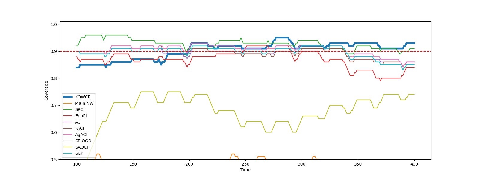
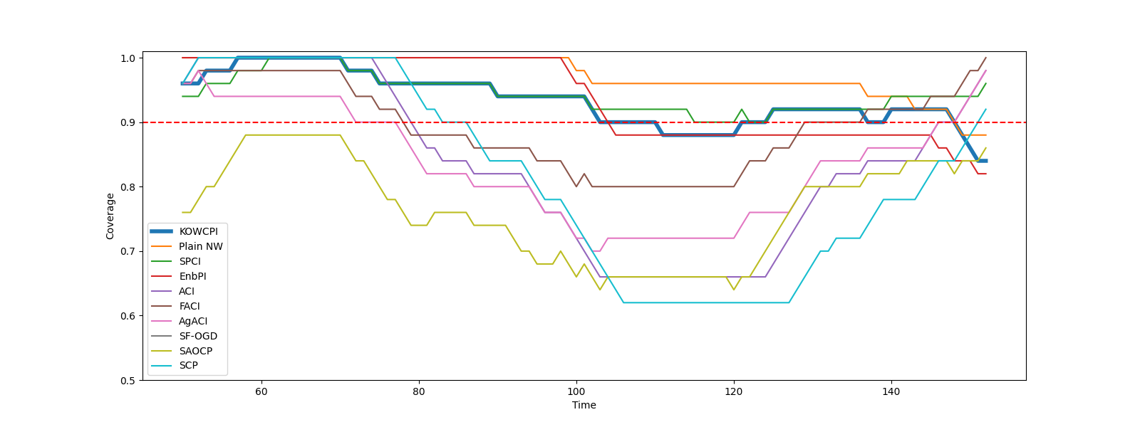
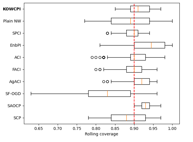
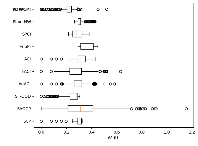
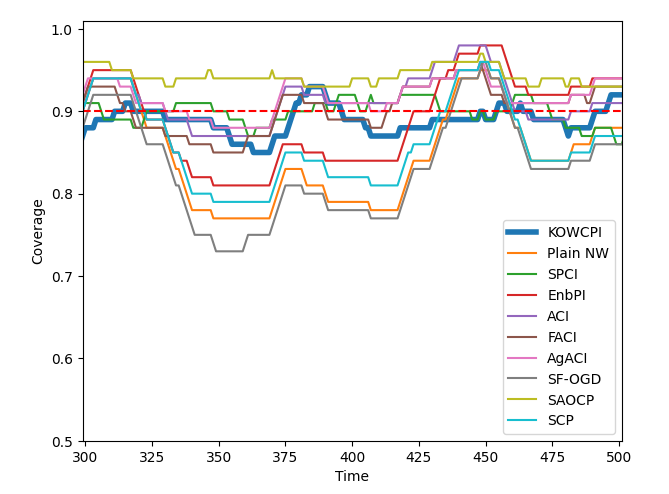
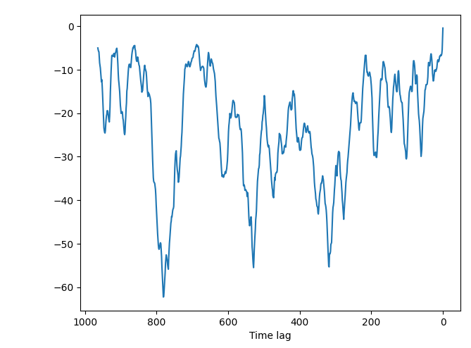
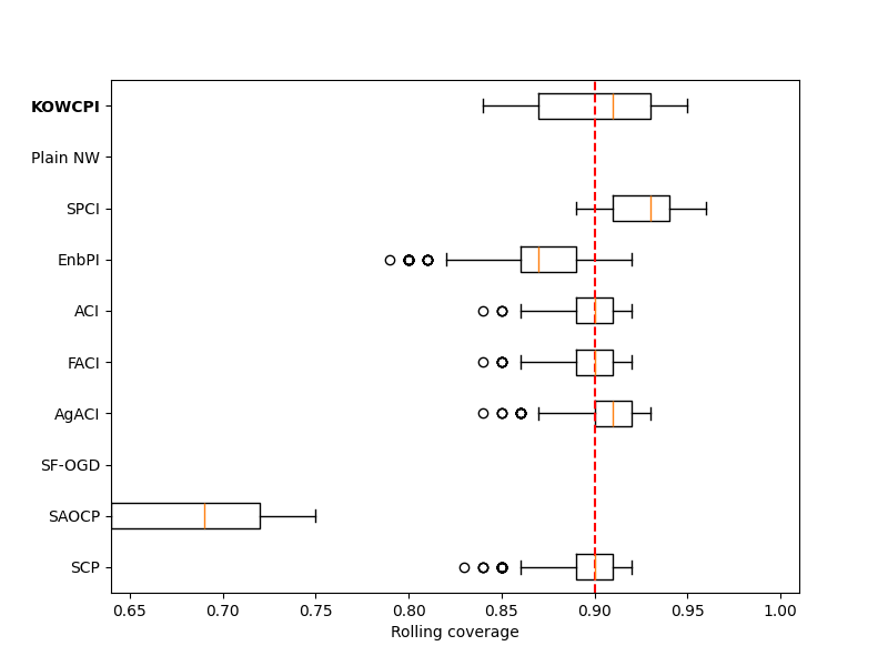
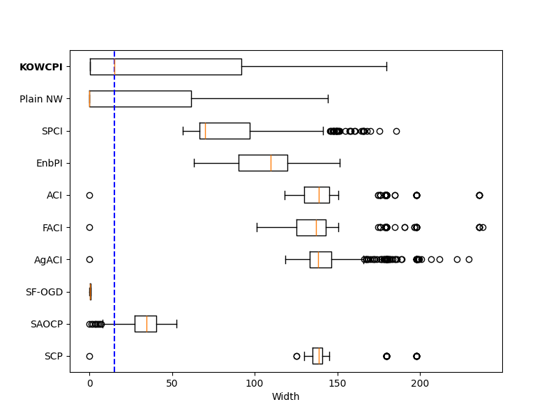
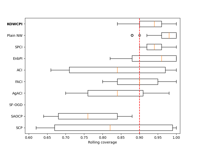
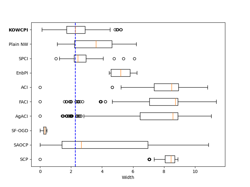
Besides examining marginal coverage and widths of prediction intervals on test data, we also focus on rolling coverage, which is helpful in showing approximate conditional coverage at specific time indices. Given a rolling window size $m>0$ , rolling coverage $\widehat{\rm RC}_{t}$ at time $t$ is defined as $\widehat{\rm RC}_{t}=\frac{1}{m}\sum_{i=1}^{m}\mathds{1}\{Y_{t-i+1}\in\widehat{C}_{t-i}^{\alpha}(X_{t-i+1})\}.$

Results. The empirical marginal coverage and width results for all methods are summarized in Table 1. The results indicate that KOWCPI consistently achieves the 90% target coverage and maintains the smallest average width compared to the alternative state-of-the-art methods. While all methods, except SF-OGD, SAOCF, and Plain NW nearly achieve marginal coverage under target $1-\alpha=0.9$ , KOWCPI produces the narrowest average width on all datasets. In terms of rolling results, we show in Figures 2 and 2 that the coverage of KOWCPI intervals consistently centers around 90% throughout the entire test phase. Additionally, Figure 2 shows that KOWCPI intervals are also significantly narrower with a smaller variance than the baselines. Lastly, Figure 2 shows weights $\widehat{W}$ (in log scale) by the RNW estimator at the first time index of test data. We note that the most recent set of non-conformity scores (in terms of time indices) receives the heaviest weighting, which is natural due to the greatest similarity between the first test datum and training data closest to it in time. In Appendix C, we show additional comparisons of KOWCPI against the baselines on the other two datasets in terms of rolling results, where KOWCPI remains consistently better.

6 Conclusion

In this paper, we introduced KOWCPI, a method to sequentially construct prediction intervals for time-series data. By incorporating the classical Reweighted Nadaraya-Watson estimator into the weighted conformal prediction framework, KOWCPI effectively adapts to the dependent structure of time-series data by utilizing data-driven adaptive weights. Our theoretical contributions include providing theoretical guarantees for the asymptotic conditional coverage of KOWCPI under strong mixing conditions and bounding the marginal and conditional coverage gaps. Empirical validation on real-world time-series datasets demonstrated the effectiveness of KOWCPI compared to state-of-the-art methods, achieving narrower prediction intervals without compromising empirical coverage.

Future work could explore adaptive window selection, where the size of the non-conformity score batch is adjusted dynamically to capture shifts in the underlying distribution. Additionally, the natural compatibility of kernel regression with multivariate data can be leveraged to expand the utility of KOWCPI for multivariate time-series data, as detailed in Appendix A. There is also potential for improving theoretical guarantees and improving practical performance by designing alternative non-conformity scores.

Acknowledgments

This work is partially supported by an NSF CAREER CCF-1650913, NSF DMS-2134037, CMMI-2015787, CMMI-2112533, DMS-1938106, DMS-1830210, and the Coca-Cola Foundation.

References

Abdous and Theodorescu [1992] B. Abdous and R. Theodorescu. Note on the spatial quantile of a random vector. Statist. Probab. Lett., 13(4):333–336, 1992.
Angelopoulos et al. [2023] A. Angelopoulos, E. Candès, and R. J. Tibshirani. Conformal PID Control for Time Series Prediction. In Advances in Neural Information Processing Systems, 2023.
Angelopoulos and Bates [2023] A. N. Angelopoulos and S. Bates. Conformal Prediction: A Gentle Introduction. Foundations and Trends® in Machine Learning, 16(4):494–591, 2023.
Auer et al. [2023] A. Auer, M. Gauch, D. Klotz, and S. Hochreiter. Conformal Prediction for Time Series with Modern Hopfield Networks. In Advances in Neural Information Processing Systems, 2023.
Barber et al. [2023] R. F. Barber, E. J. Candès, A. Ramdas, and R. J. Tibshirani. Conformal prediction beyond exchangeability. The Annals of Statistics, 51(2):816 – 845, 2023.
Bhatnagar et al. [2023] A. Bhatnagar, H. Wang, C. Xiong, and Y. Bai. Improved Online Conformal Prediction via Strongly Adaptive Online Learning. In Proceedings of the 40th International Conference on Machine Learning, 2023.
Cai [2001] Z. Cai. Weighted Nadaraya-Watson regression estimation. Statistics & Probability Letters, 51(3):307–318, 2001.
Cai [2002] Z. Cai. Regression quantiles for time series. Econometric Theory, 18(1):169–192, 2002.
Cai and Tiwari [2000] Z. Cai and R. C. Tiwari. Application of a local linear autoregressive model to BOD time series. Environmetrics, 11(3):341–350, 2000.
Fan et al. [1995] J. Fan, N. E. Heckman, and M. P. Wand. Local Polynomial Kernel Regression for Generalized Linear Models and Quasi-Likelihood Functions. Journal of the American Statistical Association, 90(429):141–150, 1995.
Feldman et al. [2022] S. Feldman, L. Ringel, S. Bates, and Y. Romano. Achieving Risk Control in Online Learning Settings. arXiv preprint arXiv:2205.09095, 2022.
Gibbs and Candès [2021] I. Gibbs and E. Candès. Adaptive Conformal Inference Under Distribution Shift. Advances in Neural Information Processing Systems, 34:1660–1672, 2021.
Gibbs and Candès [2022] I. Gibbs and E. Candès. Conformal Inference for Online Prediction with Arbitrary Distribution Shifts. arXiv preprint arXiv:2208.08401, 2022.
Gibbs et al. [2023] I. Gibbs, J. J. Cherian, and E. J. Candès. Conformal Prediction With Conditional Guarantees. arXiv preprint arXiv:2305.12616, 2023.
Guan [2023] L. Guan. Localized conformal prediction: a generalized inference framework for conformal prediction. Biometrika, 110(1):33–50, 2023.
Hall et al. [1999] P. Hall, R. C. Wolff, and Q. Yao. Methods for Estimating a Conditional Distribution Function. Journal of the American Statistical Association, 94(445):154–163, 1999.
Harries [1999] M. Harries. SPLICE-2 Comparative Evaluation: Electricity Pricing. Technical report, University of New South Wales, School of Computer Science and Engineering, 1999.
Hastie [1990] T. J. Hastie. Generalized additive models. CRC Press, 1990.
Ibragimov et al. [1971] I. A. Ibragimov, Y. V. Linnik, and J. F. C. Kingman. Independent and Stationary Sequences of Random Variables. Wolters-Noordhoff., 1971.
Kim et al. [2020] B. Kim, C. Xu, and R. Barber. Predictive inference is free with the jackknife+-after-bootstrap. Advances in Neural Information Processing Systems, 33:4138–4149, 2020.
Kivaranovic et al. [2020] D. Kivaranovic, K. D. Johnson, and H. Leeb. Adaptive, Distribution-Free Prediction Intervals for Deep Networks. In Proceedings of the Twenty Third International Conference on Artificial Intelligence and Statistics, 2020.
Lee et al. [2023] Y. Lee, R. F. Barber, and R. Willett. Distribution-free inference with hierarchical data. arXiv preprint arXiv:2306.06342, 2023.
Lei and Wasserman [2014] J. Lei and L. Wasserman. Distribution-free prediction bands for non-parametric regression. Journal of the Royal Statistical Society Series B: Statistical Methodology, 76(1):71–96, 2014.
Lei et al. [2013] J. Lei, J. Robins, and L. Wasserman. Distribution-Free Prediction Sets. Journal of the American Statistical Association, 108(501):278–287, 2013.
Masry [1986] E. Masry. Recursive probability density estimation for weakly dependent stationary processes. IEEE Transactions on Information Theory, 32(2):254–267, 1986.
Nadaraya [1964] E. A. Nadaraya. On Estimating Regression. Theory of Probability & Its Applications, 9(1):141–142, 1964.
Orabona and Pál [2018] F. Orabona and D. Pál. Scale-free online learning. Theoretical Computer Science, 716:50–69, 2018.
Romano et al. [2019] Y. Romano, E. Patterson, and E. Candès. Conformalized Quantile Regression. In Advances in Neural Information Processing Systems, 2019.
Salha [2006] R. Salha. Kernel Estimation for the Conditional Mode and Quantiles of Time Series. PhD thesis, University of Macedonia, 2006.
Sesia and Candès [2020] M. Sesia and E. J. Candès. A comparison of some conformal quantile regression methods. Stat, 9(1):e261, 2020.
Stankevičiūtė et al. [2021] K. Stankevičiūtė, A. Alaa, and M. van der Schaar. Conformal time-series forecasting. In Advances in Neural Information Processing Systems, 2021.
Steikert [2014] K. U. Steikert. The weighted Nadaraya-Watson Estimator: Strong consistency results, rates of convergence, and a local bootstrap procedure to select the bandwidth. PhD thesis, University of Zurich, 2014.
Sun and Yu [2024] S. H. Sun and R. Yu. Copula conformal prediction for multi-step time series prediction. In The Twelfth International Conference on Learning Representations, 2024.
Tibshirani et al. [2019] R. J. Tibshirani, R. Foygel Barber, E. Candès, and A. Ramdas. Conformal Prediction Under Covariate Shift. Advances in Neural Information Processing Systems, 32, 2019.
Tsybakov [2009] A. B. Tsybakov. Introduction to Nonparametric Estimation. Springer, 2009.
Tucker [1967] H. G. Tucker. A Graduate Course in Probability. Academic Press, 1967.
Vovk [2012] V. Vovk. Conditional validity of inductive conformal predictors. In Proceedings of the Asian Conference on Machine Learning, 2012.
Vovk et al. [1999] V. Vovk, A. Gammerman, and C. Saunders. Machine-Learning Applications of Algorithmic Randomness. In Proceedings of the Sixteenth International Conference on Machine Learning, 1999.
Vovk et al. [2005] V. Vovk, A. Gammerman, and G. Shafer. Algorithmic Learning in a Random World. Springer, 2005.
Wand and Jones [1994] M. P. Wand and M. C. Jones. Kernel Smoothing. CRC press, 1994.
Watson [1964] G. S. Watson. Smooth regression analysis. Sankhyā: The Indian Journal of Statistics, Series A, 26:359–372, 1964.
Xu and Xie [2021a] C. Xu and Y. Xie. Conformal Anomaly Detection on Spatio-Temporal Observations with Missing Data. arXiv preprint arXiv:2105.11886, 2021a.
Xu and Xie [2021b] C. Xu and Y. Xie. Conformal prediction interval for dynamic time-series. In Proceedings of the 38th International Conference on Machine Learning, 2021b.
Xu and Xie [2022] C. Xu and Y. Xie. Conformal prediction set for time-series. arXiv preprint arXiv:2206.07851, 2022.
Xu and Xie [2023a] C. Xu and Y. Xie. Conformal prediction for time series. IEEE Transactions on Pattern Analysis and Machine Intelligence, 45(10):11575–11587, 2023a.
Xu and Xie [2023b] C. Xu and Y. Xie. Sequential Predictive Conformal Inference for Time Series. In Proceedings of the 40th International Conference on Machine Learning, 2023b.
Xu et al. [2024] C. Xu, H. Jiang, and Y. Xie. Conformal prediction for multi-dimensional time series by ellipsoidal sets. arXiv preprint arXiv:2403.03850, 2024.
Yu and Jones [1998] K. Yu and M. C. Jones. Local Linear Quantile Regression. Journal of the American Statistical Association, 93(441):228–237, 1998.
Zaffran et al. [2022] M. Zaffran, O. Féron, Y. Goude, J. Josse, and A. Dieuleveut. Adaptive Conformal Predictions for Time Series. In Proceedings of the 39th International Conference on Machine Learning, 2022.
Zhang et al. [2021] M. Zhang, C. Xu, A. Sun, F. Qiu, and Y. Xie. Solar Radiation Ramping Events Modeling Using Spatio-temporal Point Processes. arXiv preprint arXiv:2101.11179, 2021.
Zhu et al. [2021] S. Zhu, H. Zhang, Y. Xie, and P. Van Hentenryck. Multi-resolution spatio-temporal prediction with application to wind power generation. arXiv preprint arXiv:2108.13285, 2021.

Appendix A Multivariate time series

In the main text, our discussion has centered on cases where the response variables $Y_{t}$ are scalars. Here, we explore the natural extension of our methodology to handle scenarios with multivariate responses. This extension requires defining multivariate quantiles, introducing a multivariate version of the RNW estimator for estimating these quantiles [Salha, 2006], and adapting our KOWCPI method for multivariate responses.

Multivariate conditional quantiles

Consider a strongly mixing stationary process $((\tilde{X}_{i},\tilde{Y}_{i}))_{i=1}^{\infty}$ , which is a realization of random variable $(\tilde{X},\tilde{Y})\in\mathbb{R}^{p}\times\mathbb{R}^{s}$ . Following Abdous and Theodorescu [1992], we first define a pseudo-norm function $\left\|\cdot\right\|_{2,\alpha}:\mathbb{R}^{s}\to\mathbb{R}$ for $\alpha\in(0,1)$ as

\left\|v\right\|_{2,\alpha}=\left\|\left(\frac{\left|v_{1}\right|+(2\alpha-1)}{2},\ldots,\frac{\left|v_{s}\right|+(2\alpha-1)}{2}\right)\right\|_{2},

for $v\in\mathbb{R}^{s}$ , where $\left\|\cdot\right\|_{2}$ is the Euclidean norm on $\mathbb{R}^{s}$ . Let

H_{\alpha}(\theta,\tilde{x})\coloneqq\mathbb{E}[\|\tilde{Y}-\theta\|_{2,\alpha}-\|\tilde{Y}\|_{2,\alpha}\mid\tilde{X}=\tilde{x}].

Definition A.1 (Multivariate conditional quantile [Abdous and Theodorescu, 1992]).

Define a multivariate conditional $\alpha$ -quantile $\theta_{\alpha}(\tilde{x})$ for $\alpha\in(0,1)$ as

\theta_{\alpha}(\tilde{x})=\mathop{\rm argmin}_{\theta\in\mathbb{R}^{s}}H_{\alpha}(\theta,\tilde{x}).

(A.1)

Remark A.2 (Compatibility with univariate quantile function).

For a scalar $\tilde{Y}\in\mathbb{R}$ , its conditional quantile given $\tilde{X}=\tilde{x}$ is

	$\displaystyle\theta_{\alpha}(\tilde{x})$	$\displaystyle=\mathop{\rm argmin}_{\theta\in\mathbb{R}}\mathbb{E}\left[\\|{\tilde{Y}-\theta}\\|_{2,\alpha}\mid\tilde{X}=\tilde{x}\right]$
		$\displaystyle=\mathop{\rm argmin}_{\theta\in\mathbb{R}}\mathbb{E}\left[\|{\tilde{Y}-\theta}\|+(2\alpha-1)(\tilde{Y}-\theta)\mid\tilde{X}=\tilde{x}\right]$
		$\displaystyle=\mathop{\rm argmin}_{\theta\in\mathbb{R}}\mathbb{E}((\tilde{Y}-\theta)(\alpha-\mathds{1}(\tilde{Y}\leq\theta))\mid\tilde{X}=\tilde{x})$
		$\displaystyle=Q_{\alpha}(\tilde{x}),$

for any $\alpha\in(0,1)$ . Thus, Definition A.1 is consistent with the univariate case.

Multivariate RNW estimator

Following the definition in (6), we obtain the RNW estimator for multivariate responses as

\widehat{F}(\tilde{y}|\tilde{x})=\frac{\sum_{i=1}^{n}W(\frac{\tilde{X}_{i}-\tilde{x}}{h})\mathds{1}(\tilde{Y}_{i}\leq\tilde{y})}{\sum_{i=1}^{n}W(\frac{\tilde{X}_{i}-\tilde{x}}{h})},

(A.2)

where, according to (7) and (8),

W(u)=\frac{K(u)}{1+\lambda u_{1}K(u)},

for $u=(u_{1},\ldots,u_{p})^{\top}$ . Now, let $W_{h}(u)=h^{-p}W(h^{-1}u)$ , and define an estimator for $H_{\alpha}(\theta,x)$ as

\widehat{H}_{\alpha}(\theta,\tilde{x})\coloneqq\int_{\mathbb{R}^{s}}(\|{\tilde{y}-\theta}\|_{2,\alpha}-\|{\tilde{y}}\|_{2,\alpha})\widehat{F}(d\tilde{y}|\tilde{x})=\frac{\sum_{i=1}^{n}W_{h}(\tilde{X}_{i}-\tilde{x})\left(\|{\tilde{Y}_{i}-\theta}\|_{2,\alpha}-\|{\tilde{Y}_{i}}\|_{2,\alpha}\right)}{\sum_{i=1}^{n}W_{h}(\tilde{X}_{i}-\tilde{x})},

and consequently the RNW conditional quantile estimator $\widehat{\theta}_{\alpha}$ as

\displaystyle\begin{split}\widehat{\theta}_{\alpha}(\tilde{x})\coloneqq\mathop{\rm argmin}_{\theta\in\mathbb{R}^{p}}\hat{H}_{\alpha}(\theta,\tilde{x})=\mathop{\rm argmin}_{\theta\in\mathbb{R}^{p}}\sum_{i=1}^{n}W_{h}(\tilde{X}_{i}-\tilde{x})(\|{\tilde{Y}_{i}-\theta}\|_{2,\alpha}-\|{\tilde{Y}_{i}}\|_{2,\alpha}).\end{split}

(A.3)

Multivariate KOWCPI

Suppose we are sequentially observing $(X_{t},Y_{t})\in\mathbb{R}^{d}\times\mathbb{R}^{s}$ , $t=1,2,\ldots$ . Based on the construction of the multivariate version of the RNW estimator, we can extend our KOWCPI approach to multivariate responses in the same manner as described in Algorithm 1, with multivariate residuals

\hat{\varepsilon}_{t}=Y_{t}-\hat{f}(X_{t})\in\mathbb{R}^{s},

as non-conformity scores. This adaptation allows for the application of our methodology to a broader range of data scenarios involving dependent data with multivariate response variables, which were similarly studied in [Xu et al., 2024, Sun and Yu, 2024, Stankevičiūtė et al., 2021].

Appendix B Proofs

The following lemma is adapted from the proof of Lemma 1 of Tibshirani et al. [2019]; however, we do not assume exchangeability.

Lemma B.1 (Weights on quantile for non-exchangeable data).

Given a sequence of random variables $\{V_{1},\ldots,V_{n+1}\}$ with joint density $\mathcal{P}$ and a sequence of observations $\{v_{1},\ldots,v_{n+1}\}$ . Define the event

E=\{\{V_{1},\ldots,V_{n+1}\}=\{v_{1},\ldots,v_{n+1}\}\}.

Then we have for $i=1,\ldots,n+1$ ,

\mathbb{P}\{V_{n+1}=v_{i}|E\}=\frac{\sum_{\sigma:\sigma(n+1)=i}\mathcal{P}(v_{\sigma(1)},\ldots,v_{\sigma(n+1)})}{\sum_{\sigma}\mathcal{P}(v_{\sigma(1)},\ldots,v_{\sigma(n+1)})}\in[0,1].

Note that when the residuals are exchangeable, $W_{i}^{*}=1/(n+1)$ , as also observed in Tibshirani et al. [2019]. Now we prove Proposition 4.1.

Proof of Proposition 4.1.

The proof assumes that $\tilde{Y}_{i}$ , for $i=1,\ldots,n+1$ , are almost surely distinct. However, the proof remains valid, albeit with more complex notations involving multisets, if this is not the case. Denote by ${\rm Quantile}_{\beta}(\mathbb{Q})$ the $\beta$ -quantile of the distribution $\mathbb{Q}$ on $\mathbb{R}$ , and by $\delta_{a}$ the point mass distribution at $a\in\mathbb{R}$ . Define the event $E=\{\{\tilde{Y}_{1},\ldots,\tilde{Y}_{n+1}\}=\{v_{1},\ldots,v_{n+1}\}\}$ . Then, by the tower property, we have

	$\displaystyle\mathbb{P}(Y_{T+1}\in\widehat{C}_{T}^{\alpha}(X_{T+1}))$
	$\displaystyle=\mathbb{E}(\mathbb{P}(Y_{T+1}\in\widehat{C}_{T}^{\alpha}(X_{T+1})\mid E))$
	$\displaystyle=\left.\mathbb{E}\left[\mathbb{P}\left({\rm Quantile}_{\beta^{}}\left(\sum_{i=1}^{n}\widehat{W}_{i}\delta_{v_{i}}\right)\leq\tilde{Y}_{n+1}\leq{\rm Quantile}_{1-\alpha+{\beta^{}}}\left(\sum_{i=1}^{n}\widehat{W}_{i}\delta_{v_{i}}\right)\right\|E\right)\right]$
	$\displaystyle=\mathbb{E}\left[\mathbb{P}_{V\sim P^{W^{}}}\left({\rm Quantile}_{\beta^{}}\left(\sum_{i=1}^{n}\widehat{W}_{i}\delta_{v_{i}}\right)\leq V\leq{\rm Quantile}_{1-\alpha+{\beta^{*}}}\left(\sum_{i=1}^{n}\widehat{W}_{i}\delta_{v_{i}}\right)\right)\right],$

where $P^{W^{*}}=\sum_{i=1}^{n+1}W^{*}_{i}\delta_{v_{i}}$ , and in the last line, we have used the result from Lemma B.1,

\tilde{Y}_{n+1}|E\sim P^{W^{*}}.

Denote the weighted empirical distributions based on $\widehat{W}=\widehat{W}(\tilde{X}_{n+1})$ as

\displaystyle P^{\widehat{W}}

\displaystyle=\sum_{i=1}^{n}\widehat{W}_{i}\delta_{v_{i}}.

This gives the marginal coverage gap as

	$\displaystyle\left\|\mathbb{P}(Y_{n+1}\in\widehat{C}_{n}^{\alpha}(X_{n+1}))-(1-\alpha)\right\|$
	$\displaystyle\leq\mathbb{E}\left[\left\|\mathbb{P}_{V\sim P^{W^{}}}\Bigg{(}{\rm Quantile}_{\beta^{}}\left(\sum_{i=1}^{n}\widehat{W}_{i}\delta_{v_{i}}\right)\leq V\leq{\rm Quantile}_{1-\alpha+{\beta^{*}}}\left(\sum_{i=1}^{n}\widehat{W}_{i}\delta_{v_{i}}\right)\Bigg{)}\right.\right.$
	$\displaystyle\quad\quad\left.-\left.\mathbb{P}_{V\sim P^{\widehat{W}}}\left({\rm Quantile}_{\beta^{}}\left(\sum_{i=1}^{n}\widehat{W}_{i}\delta_{v_{i}}\right)\leq V\leq{\rm Quantile}_{1-\alpha+{\beta^{}}}\left(\sum_{i=1}^{n}\widehat{W}_{i}\delta_{v_{i}}\right)\right)\right\|\right]$
	$\displaystyle\quad+\mathbb{E}\left\|\mathbb{P}_{V\sim P^{\widehat{W}}}\left({\rm Quantile}_{\beta^{}}\left(\sum_{i=1}^{n}\widehat{W}_{i}\delta_{v_{i}}\right)\leq V\leq{\rm Quantile}_{1-\alpha+{\beta^{}}}\left(\sum_{i=1}^{n}\widehat{W}_{i}\delta_{v_{i}}\right)\right)-(1-\alpha)\right\|$
	$\displaystyle\leq\mathbb{E}[d_{\rm TV}(P^{W^{*}},P^{\widehat{W}})]$
	$\displaystyle\quad+\mathbb{E}\left\|\widehat{F}\left(\widehat{Q}_{1-\alpha+{\beta^{}}}(\tilde{X}_{n+1})\Big{\|}\tilde{X}_{n+1}\right)-(1-\alpha+{\beta^{}})\right\|+\mathbb{E}\left\|\widehat{F}\left(\widehat{Q}_{{\beta^{}}}(\tilde{X}_{n+1})\Big{\|}\tilde{X}_{n+1}\right)-{\beta^{}}\right\|$
	$\displaystyle\leq\frac{1}{2}\mathbb{E}\\|(W^{})_{1:n}-\widehat{W}\\|_{1}+\frac{1}{2}\mathbb{E}W^{}_{n+1}+2\mathbb{E}\max_{i=1,\ldots,n}\widehat{W}_{i}(\tilde{X}_{n+1}),$

where we denote by $d_{\rm TV}(\cdot,\cdot)$ the total variation distance between probability measures, and the second inequality is due to the definition of the total variation distance. ∎

B.1 Proof of asymptotic conditional coverage of KOWCPI (Corollary 4.8 and Theorem 4.9)

In deriving the asymptotic conditional coverage property of KOWCPI, the consistency of the RNW estimator plays a crucial role. Therefore, we first introduce the proof of Proposition 4.6, which discusses the consistency of the CDF estimator. Corollary 4.7, which states the consistency of the quantile estimator, is a natural consequence of Proposition 4.6 and leads us to the proof for our main results, Corollary 4.8 and Theorem 4.9. Proof of Proposition 4.6 adopts the similar strategy as Salha [2006] and Cai [2002].

To prove Proposition 4.6, it is essential to first understand the nature of the adjustment weight $p_{i}(\mathbf{z})$ . Thus, Lemma 3.1 is not only crucial for the practical implementation of the RNW estimator but also indispensable in the proof process of Proposition 4.6.

Proof of Lemma 3.1.

For display purposes, denote $[X]_{1}$ as $X_{1}$ . By (5), we have that

\sum_{i=1}^{n}p_{i}(\mathbf{z})(\tilde{X}_{i1}-\tilde{x}_{1})K_{h}(\tilde{X}_{i}-\mathbf{z})=0.

(A.4)

Let

	$\displaystyle\mathcal{L}(\lambda_{1},\lambda_{2},p_{1}(\mathbf{z}),\ldots,p_{n}(\mathbf{z}))$
	$\displaystyle=\sum_{i=1}^{n}\log p_{i}(\mathbf{z})+\lambda_{1}\Bigg{(}1-\sum_{i=1}^{n}p_{i}(\mathbf{z})\Bigg{)}+\lambda_{2}\sum_{i=1}^{n}p_{i}(\mathbf{z})(\tilde{X}_{i1}-\tilde{x}_{1})K_{h}(\tilde{X}_{i}-\mathbf{z}),$

where $\lambda_{1},\lambda_{2}\in\mathbb{R}$ are the Lagrange multipliers. From $\partial\mathcal{L}/\partial p_{i}(\mathbf{z})=0$ for $i=1,\ldots,n$ , we get

\displaystyle p_{i}^{-1}(\mathbf{z})-\lambda_{1}+\lambda_{2}(\tilde{X}_{i1}-\tilde{x}_{1})K_{h}(\tilde{X}_{i}-\mathbf{z})=0,

Since $p_{i}(\mathbf{z})$ ’s sum up to 1 as in (4), letting $\lambda=-\lambda_{2}/\lambda_{1}$ , we have

p_{i}(\mathbf{z})=\frac{[1+\lambda(\tilde{X}_{i1}-\tilde{x}_{1})K_{h}(\tilde{X}_{i}-\mathbf{z})]^{-1}}{\sum_{j=1}^{n}[1+\lambda(\tilde{X}_{j1}-\tilde{x}_{1})K_{h}(\tilde{X}_{j}-\mathbf{z})]^{-1}}.

Using (4) again with (A.4), this gives

\displaystyle\sum_{j=1}^{n}\left[1+\lambda(\tilde{X}_{j1}-\tilde{x}_{1})K_{h}(\tilde{\mathbf{X}}_{j}-\mathbf{z})\right]^{-1}=n\Bigg{(}\sum_{i=1}^{n}p_{i}(\mathbf{z})[1+\lambda(\tilde{X}_{i1}-\tilde{x}_{1})K_{h}(\tilde{X}_{i}-\mathbf{z})]\Bigg{)}^{-1}=n,

and therefore (8) holds. With (5), this gives

0=\sum_{i=1}^{n}\frac{(\tilde{X}_{i1}-\tilde{x}_{1})K_{h}(\tilde{X}_{i}-\mathbf{z})}{1+\lambda(\tilde{X}_{i1}-\tilde{x}_{1})K_{h}(\tilde{X}_{i}-\mathbf{z})}=\left.-\frac{\partial L(\gamma;\mathbf{z})}{\partial\gamma}\right|_{\lambda}.

Note that $\frac{\partial^{2}L(\gamma;\mathbf{z})}{\partial{\gamma}^{2}}\geq 0$ , implying that $L(\cdot;\mathbf{z})$ is indeed a convex function. ∎

Lemma B.2.

Under the assumptions of Proposition 4.6, define

c(\mathbf{z})=\frac{\frac{\partial g(\mathbf{z})}{\partial\tilde{x}_{1}}\mu_{2}}{g(\mathbf{z})\nu_{2}}.

Then,

\lambda=h^{w}\cdot c(\mathbf{z})(1+o_{p}(1))=\mathcal{O}_{p}(h^{w}).

(A.5)

Proof.

Let

S_{i}=(\tilde{X}_{i1}-\tilde{x}_{1})K_{h}(\tilde{X}_{i}-\mathbf{z}).

Then, by Assumption 4.4, $S_{i}$ is bounded above by some constant $C_{1}$ . Let

\overline{S^{k}}=\frac{1}{n}\sum_{i=1}^{n}(S_{i})^{k},

for $k=1,2$ . Then, from (A.4), we have

\displaystyle 0

\displaystyle=\frac{1}{n}\sum_{i=1}^{n}(1+\lambda S_{i})^{-1}S_{i}\geq\left|\lambda\right|\left|\frac{1}{n}\sum_{i=1}^{n}S_{i}^{2}(1+\lambda S_{i})^{-1}\right|-\left|\overline{S^{1}}\right|\geq\left|\lambda\right|(1+C_{1}\left|\lambda\right|)^{-1}\overline{S^{2}}-\left|\overline{S^{1}}\right|,

which gives

\left|\lambda\right|\leq\frac{\left|\overline{S^{1}}\right|}{\overline{S^{2}}-C_{1}\left|\overline{S^{1}}\right|}.

Using the Taylor expansion [Wand and Jones, 1994], we obtain that

	$\displaystyle\mathbb{E}\overline{S^{1}}$	$\displaystyle=\int_{\mathbb{R}^{w}}(u_{1}-\tilde{x}_{1})K_{h}(\mathbf{u}-\mathbf{z})g(\mathbf{u})d\mathbf{u}$
		$\displaystyle=h\int_{\mathbb{R}^{w}}u_{1}K(\mathbf{u})g(\mathbf{z}+h\mathbf{u})d\mathbf{u}$
		$\displaystyle=h\int_{\mathbb{R}^{w}}u_{1}K(\mathbf{u})\Bigg{(}g(\mathbf{z})+h\sum_{j=1}^{w}u_{j}\frac{\partial g(\mathbf{z})}{\partial\tilde{x}_{j}}\Bigg{)}d\mathbf{u}+o(h^{2})$
		$\displaystyle=h^{2}\left\{\frac{\partial g(\mathbf{z})}{\partial\tilde{x}_{1}}\mu_{2}+o_{p}(1)\right\},$

where the last equation comes from Assumptions 4.4-(i) and (ii). With a similar argument, we can derive that

\displaystyle\mathbb{E}\overline{S^{2}}

\displaystyle=\int_{\mathbb{R}^{w}}(u_{1}-\tilde{x}_{1})^{2}K_{h}^{2}(\mathbf{u}-\mathbf{z})g(\mathbf{u})d\mathbf{u}=h^{-w+2}\left\{g(\mathbf{z})\nu_{2}+o_{p}(h)\right\},

using Assumption 4.4-(iii). Therefore, we obtain (A.5). ∎

Decomposing $\widehat{F}(\tilde{y}|\mathbf{z})-F(\tilde{y}|\mathbf{z})$ in bias and variance terms, we get

	$\displaystyle\widehat{F}(\tilde{y}\|\mathbf{z})-F(\tilde{y}\|\mathbf{z})$
	$\displaystyle=\frac{\sum_{i=1}^{n}p_{i}(\mathbf{z})K_{h}(\tilde{X}_{i}-\mathbf{z})\{\mathds{1}(\tilde{Y}_{i}<\tilde{y})-F(\tilde{y}\|\mathbf{z})\}}{\sum_{i=1}^{n}p_{i}(\mathbf{z})K_{h}(\tilde{X}_{i}-\mathbf{z})}$
	$\displaystyle=\frac{\sum_{i=1}^{n}p_{i}(\mathbf{z})K_{h}(\tilde{X}_{i}-\mathbf{z})\delta_{i}+\sum_{i=1}^{n}p_{i}(\mathbf{z})K_{h}(\tilde{X}_{i}-\mathbf{z})\{F(\tilde{y}\|\tilde{X}_{i})-F(\tilde{y}\|\mathbf{z})\}}{\sum_{i=1}^{n}p_{i}(\mathbf{z})K_{h}(\tilde{X}_{i}-\mathbf{z})},$

where $\delta_{i}=\mathds{1}(\tilde{Y}_{t}\leq\tilde{y})-F(\tilde{y}|\tilde{X}_{i})$ . Note that $\mathbb{E}[\delta_{i}]=0$ due to the tower property. Now, let

b_{i}(\mathbf{z})=b_{i}(\tilde{X}_{i},\mathbf{z})\coloneqq\left[1+h^{w}\cdot c(\mathbf{z})(\tilde{X}_{i1}-\tilde{x}_{1})K_{h}(\tilde{X}_{i}-\mathbf{z})\right]^{-1}.

Then, by Lemma B.2, we have that

p_{i}(\mathbf{z})=n^{-1}b_{i}(\mathbf{z})(1+o_{p}(1)).

(A.6)

Define

	$\displaystyle J_{1}=n^{-1/2}h^{w/2}\sum_{i=1}^{n}b_{i}(\mathbf{z})\delta_{i}K_{h}(\tilde{X}_{i}-\mathbf{z}),$
	$\displaystyle J_{2}=n^{-1}\sum_{i=1}^{n}\left\{F(\tilde{y}\|\tilde{X}_{i})-F(\tilde{y}\|\mathbf{z})\right\}b_{i}(\mathbf{z})K_{h}(\tilde{X}_{i}-\mathbf{z}),$
	$\displaystyle J_{3}=n^{-1}\sum_{i=1}^{n}b_{i}(\mathbf{z})K_{h}(\tilde{X}_{i}-\mathbf{z}),$

so that

\widehat{F}(\tilde{y}|\mathbf{z})-F(\tilde{y}|\mathbf{z})=\{(nh^{w})^{-1/2}J_{1}+J_{2}\}J_{3}^{-1}\{1+o_{p}(1)\}.

(A.7)

Therefore, we will derive Proposition 4.6 by controlling the terms $J_{1}$ , $J_{2}$ and $J_{3}$ .

Lemma B.3.

Under the assumptions of Proposition 4.6,

J_{1}=\mathcal{O}_{p}(1).

(A.8)

Proof.

Let

\xi_{i}=h^{w/2}b_{i}(\mathbf{z})\delta_{i}K_{h}(\tilde{X}_{i}-\mathbf{z}),

so that $J_{1}=n^{-1/2}\sum_{i=1}^{n}\xi_{i}$ . Since $\mathbb{E}(\delta_{i}|\tilde{X}_{i})=0$ , we have that $\mathbb{E}(\xi_{i})=\mathbb{E}(\mathbb{E}(\xi_{i}|\tilde{X}_{i}))=0$ , and thus

\displaystyle\mathbb{E}J_{1}=0.

(A.9)

Also, due to the stationarity of $\tilde{X}_{i}$ , we have that

\mbox{Var}(J_{1})=\mathbb{E}\xi_{i}^{2}+\sum_{i=2}^{n}\left(1-\frac{i-1}{n}\right)\mbox{Cov}(\xi_{1},\xi_{i}).

(A.10)

By Assumption 4.4, we have that $\lim_{n\to\infty}b_{i}(\mathbf{z})=1$ , which gives $\mathbb{E}(b_{i})=1+o_{p}(1)$ . Therefore, through expansion, we have

	$\displaystyle\mathbb{E}\xi_{i}^{2}$	$\displaystyle=h^{w}\mathbb{E}\left[\mathbb{E}\left[b_{i}^{2}(\mathbf{z})K_{h}^{2}(\tilde{X}_{i}-\mathbf{z})\delta_{i}^{2}\mid\tilde{X}_{i}\right]\right]$
		$\displaystyle=h^{w}\mathbb{E}\left[b_{i}^{2}(\mathbf{z})K_{h}^{2}(\tilde{X}_{i}-\mathbf{z})F(\tilde{y}\|\tilde{X}_{i})(1-F(\tilde{y}\|\tilde{X}_{i}))\right]$
		$\displaystyle=\left[(K^{2})_{h}\ast\{b_{i}^{2}(\cdot,\mathbf{z})F(\tilde{y}\|\cdot)(1-F(\tilde{y}\|\cdot))g(\cdot)\}\right](\mathbf{z})$
		$\displaystyle=\nu_{0}F(\tilde{y}\|\mathbf{z})(1-F(\tilde{y}\|\mathbf{z}))g(\mathbf{z})+o_{p}(1),$

where $\ast$ in the third line is the convolution operator. To control the second term in the right-hand side of (A.10), we borrow the idea of Masry [1986]. Choose $d_{n}=\mathcal{O}(h^{-\frac{w}{1+\delta/2}})$ and decompose

\displaystyle\sum_{i=2}^{n}\left(1-\frac{i-1}{n}\right)\mbox{Cov}(\xi_{1},\xi_{i})=\sum_{i=2}^{d_{n}}\left(1-\frac{i-1}{n}\right)\mbox{Cov}(\xi_{1},\xi_{i})+\sum_{i=d_{n}+1}^{n}\left(1-\frac{i-1}{n}\right)\mbox{Cov}(\xi_{1},\xi_{i}).

We have that $\left|b_{i}(\mathbf{z})\delta_{i}\right|\leq C_{2}$ for some constant $C_{2}$ . By Assumption 4.3-(iv), we obtain

	$\displaystyle\left\|\mbox{Cov}(\xi_{1},\xi_{i})\right\|$	$\displaystyle=\left\|\int_{\mathbb{R}^{w}}\int_{\mathbb{R}^{w}}\xi_{1}\xi_{i}g_{1,i}(\mathbf{u},v)d\mathbf{u}dv-\int_{\mathbb{R}^{w}}\xi_{1}g(\mathbf{u})d\mathbf{u}\int_{\mathbb{R}^{w}}\xi_{i}g(v)dv\right\|$
		$\displaystyle\leq C_{2}^{2}h^{w}\int_{\mathbb{R}^{w}}\int_{\mathbb{R}^{w}}K(\mathbf{u})K(v)\left\|g_{1,i}(\mathbf{z}-h\mathbf{u},\mathbf{z}-hv)-g(\mathbf{z}-h\mathbf{u})g(\mathbf{z}-hv)\right\|d\mathbf{u}dv$
		$\displaystyle\leq C_{2}^{2}Mh^{w},$

so that

\sum_{i=2}^{d_{n}}\left(1-\frac{i-1}{n}\right)\mbox{Cov}(\xi_{1},\xi_{i})=\mathcal{O}_{p}(d_{n}h^{w})=o_{p}(1).

By Assumption 4.4, we have $\|(\tilde{X}_{i}-\mathbf{z})K_{h}(\tilde{X}_{i}-\mathbf{z})\|\leq C_{3}$ , so that $\left|\xi_{i}\right|\leq Ch^{-w/2}$ . Then, by Theorem 17.2.1 of Ibragimov et al. [1971], we have that

\left|\mbox{Cov}(\xi_{1},\xi_{i})\right|\leq Ch^{-w}\alpha(i-1).

Thus, we get

\displaystyle\sum_{i=d_{n}+1}^{n}\left(1-\frac{i-1}{n}\right)\mbox{Cov}(\xi_{1},\xi_{i})\leq Ch^{-w}\sum_{i\geq d_{n}}\alpha(i)\leq Ch^{-w}d_{n}^{-1-\delta}=o(1).

Therefore, we obtain

J_{1}=\mathbb{E}J_{1}+\mathcal{O}_{p}\left(\sqrt{\mbox{Var}(J_{1})}\right)=\mathcal{O}_{p}(1).

(A.11)

∎

Lemma B.4.

Under the assumptions of Proposition 4.6,

	$\displaystyle J_{2}$	$\displaystyle=\frac{1}{2}h^{2}\mu_{2}\mbox{tr}(D_{\mathbf{z}}^{2}F(\tilde{y}\|\mathbf{z}))g(\mathbf{z})+o_{p}(h^{2}),$		(A.12)
	$\displaystyle J_{3}$	$\displaystyle=g(\mathbf{z})+o_{p}(1).$		(A.13)

Proof.

By Assumption 1, (4) and (5), we have through expansion that

\displaystyle J_{2}=(2n)^{-1}\sum_{i=1}^{n}(\tilde{X}_{i}-\mathbf{z})^{\top}(D_{\mathbf{z}}^{2}F(\tilde{y}|\mathbf{z}))(\tilde{X}_{i}-\mathbf{z})b_{i}(\mathbf{z})K_{h}(\tilde{X}_{i}-\mathbf{z})+o_{p}(h^{2}).

Since

	$\displaystyle\mathbb{E}[(\tilde{X}_{i}-\mathbf{z})^{\top}D_{\mathbf{z}}^{2}F(\tilde{y}\|\mathbf{z})(\tilde{X}_{i}-\mathbf{z})b_{i}(\mathbf{z})K_{h}(\tilde{X}_{i}-\mathbf{z})]$
	$\displaystyle=\mbox{tr}(D_{\mathbf{z}}^{2}F(\tilde{y}\|\mathbf{z})\mathbb{E}[(\tilde{X}_{i}-\mathbf{z})(\tilde{X}_{i}-\mathbf{z})^{\top}b_{i}(\mathbf{z})K_{h}(\tilde{X}_{i}-\mathbf{z})])$
	$\displaystyle=h^{2}\mu_{2}g(\mathbf{z})\mbox{tr}(D_{\mathbf{z}}^{2}F(\tilde{y}\|\mathbf{z}))+o_{p}(h^{2}),$

we have

J_{2}=\frac{1}{2}h^{2}\mu_{2}\mbox{tr}(D_{\mathbf{z}}^{2}F(\tilde{y}|\mathbf{z}))g(\mathbf{z})+o_{p}(h^{2}).

(A.14)

Finally, by applying the expansion argument routinely, we get

J_{3}=g(\mathbf{z})+o_{p}(1).

(A.15)

∎

Proof of Proposition 4.6 [Cai, 2002, Salha, 2006].

Combining Lemmas B.3 and B.4 with (A.7), Assumption 4.5 gives the result. ∎

Proof of Corollary 4.7 [Cai, 2002].

Given $\mathbf{z}$ , Proposition 4.6 implies uniform convergence of $\widehat{F}(\cdot|\mathbf{z})$ to $F(\cdot|\mathbf{z})$ in probability [Tucker, 1967, p.127-128] since $F(\cdot|\mathbf{z})$ is a CDF. That is,

\sup_{\tilde{y}\in\mathbb{R}}\left|\widehat{F}(\tilde{y}|\mathbf{z})-F(\tilde{y}|\mathbf{z})\right|\to 0\mbox{ in probability}.

Given $\varepsilon>0$ , let $\delta=\delta(\varepsilon)\coloneqq\min\{\beta-F(Q_{\beta}(\mathbf{z})-\varepsilon|\mathbf{z}),F(Q_{\beta}(\mathbf{z})+\varepsilon|\mathbf{z})-\beta\}$ . Note that $\delta>0$ due to the uniqueness of the quantile. We have

	$\displaystyle\mathbb{P}\left(\left\|\widehat{Q}_{\beta}(\mathbf{z})-Q_{\beta}(\mathbf{z})\right\|>\varepsilon\right)$	$\displaystyle\leq\mathbb{P}\left(\left\|F(\widehat{Q}_{\beta}(\mathbf{z})\|\mathbf{z})-\beta\right\|>\delta\right)$
		$\displaystyle\leq\mathbb{P}\left(\sup_{\tilde{y}\in\mathbb{R}}\left\|\widehat{F}(\tilde{y}\|\mathbf{z})-F(\tilde{y}\|\mathbf{z})\right\|>\delta\right).$

The uniform convergence of $\widehat{F}(\cdot|\tilde{x})$ in probability gives the result. ∎

Proof of Corollary 4.8.

From the definition of $\hat{C}_{t-1}^{\alpha}$ in (3), we have

	$\displaystyle\mathbb{P}\left(Y_{t}\in\hat{C}_{t-1}^{\alpha}(X_{t})\Big{\|}X_{t}\right)$	$\displaystyle=\mathbb{P}\left(\tilde{Y}_{n+1}\in\left[\widehat{Q}_{\beta^{}}(\tilde{X}_{n+1}),\widehat{Q}_{1-\alpha+\beta^{}}(\tilde{X}_{n+1})\right]\Big{\|}\,\tilde{X}_{n+1}\right)$
		$\displaystyle=F\left(\widehat{Q}_{1-\alpha+\beta^{}}(\tilde{X}_{n+1})\Big{\|}\tilde{X}_{n+1}\right)-F\left(\widehat{Q}_{\beta^{}}(\tilde{X}_{n+1})\Big{\|}\tilde{X}_{n+1}\right).$

By Theorem 4.7, we have the consistency of $\widehat{Q}_{\beta}$ for all $\beta\in(0,1)$ . On that, the continuous mapping theorem and Assumption 4.3 gives

	$\displaystyle F\left(\widehat{Q}_{1-\alpha+\beta^{}}(\tilde{X}_{n+1})\Big{\|}\tilde{X}_{n+1}\right)-F\left(\widehat{Q}_{\beta^{}}(\tilde{X}_{n+1})\Big{\|}\tilde{X}_{n+1}\right)$
	$\displaystyle\to F\left(Q_{1-\alpha+\beta^{}}(\tilde{X}_{n+1})\Big{\|}\tilde{X}_{n+1}\right)-F\left(Q_{\beta^{}}(\tilde{X}_{n+1})\Big{\|}\tilde{X}_{n+1}\right)$
	$\displaystyle=1-\alpha,$

where the convergence is in probability. ∎

Proof of Theorem 4.9.

From the definition of $\widehat{C}_{t-1}^{\alpha}$ in (3), we have

	$\displaystyle\left\|\mathbb{P}\left(Y_{t}\in\widehat{C}_{t-1}^{\alpha}(x)\Big{\|}X_{t}=x\right)-(1-\alpha)\right\|$
	$\displaystyle=\left\|\mathbb{P}\left(\tilde{Y}_{n+1}\in\left[\widehat{Q}_{\beta^{}}(\tilde{x}),\widehat{Q}_{1-\alpha+\beta^{}}(\tilde{x})\right]\Big{\|}\ \tilde{X}_{n+1}=\tilde{x}\right)-(1-\alpha)\right\|$
	$\displaystyle=\left\|F\left(\widehat{Q}_{1-\alpha+\beta^{}}(\tilde{x})\Big{\|}\tilde{X}_{n+1}=\tilde{x}\right)-F\left(\widehat{Q}_{\beta^{}}(\tilde{x})\Big{\|}\tilde{X}_{n+1}=\tilde{x}\right)-(1-\alpha)\right\|$
	$\displaystyle\leq\left\|\widehat{F}\left(\widehat{Q}_{1-\alpha+\beta^{}}(\tilde{x})\Big{\|}\tilde{X}_{n+1}=\tilde{x}\right)-(1-\alpha+\beta^{})\right\|+\left\|\widehat{F}\left(\widehat{Q}_{\beta^{}}(\tilde{x})\Big{\|}\tilde{X}_{n+1}=\tilde{x}\right)-\beta^{}\right\|$
	$\displaystyle\quad+\left\|F\left(\widehat{Q}_{1-\alpha+\beta^{}}(\tilde{x})\Big{\|}\tilde{X}_{n+1}=\tilde{x}\right)-\widehat{F}\left(\widehat{Q}_{1-\alpha+\beta^{}}(\tilde{x})\Big{\|}\tilde{X}_{n+1}=\tilde{x}\right)\right\|$
	$\displaystyle\quad+\left\|F\left(\widehat{Q}_{\beta^{}}(\tilde{x})\Big{\|}\tilde{X}_{n+1}=\tilde{x}\right)-\widehat{F}\left(\widehat{Q}_{\beta^{}}(\tilde{x})\Big{\|}\tilde{X}_{n+1}=\tilde{x}\right)\right\|$
	$\displaystyle\leq 2\Delta(\tilde{x})+\mathcal{O}_{p}((nh^{w})^{-1/2}+h^{2}),$

where the last inequality comes from (A.7) and the definition of the discrete gap $\Delta$ . ∎

Appendix C Additional experiment results

We show additional rolling comparison on the solar (Figure A.1) and wind dataset (Figure A.2), where the setup and conclusions remain consistent with those on the electric dataset (Figure 2).

	$\displaystyle\left\|\mathbb{P}(Y_{n+1}\in\widehat{C}_{n}^{\alpha}(X_{n+1}))-(1-\alpha)\right\|$
	$\displaystyle\leq\mathbb{E}\left[\left\|\mathbb{P}_{V\sim P^{W^{}}}\Bigg{(}{\rm Quantile}_{\beta^{}}\left(\sum_{i=1}^{n}\widehat{W}_{i}\delta_{v_{i}}\right)\leq V\leq{\rm Quantile}_{1-\alpha+{\beta^{*}}}\left(\sum_{i=1}^{n}\widehat{W}_{i}\delta_{v_{i}}\right)\Bigg{)}\right.\right.$
	$\displaystyle\quad\quad\left.-\left.\mathbb{P}_{V\sim P^{\widehat{W}}}\left({\rm Quantile}_{\beta^{}}\left(\sum_{i=1}^{n}\widehat{W}_{i}\delta_{v_{i}}\right)\leq V\leq{\rm Quantile}_{1-\alpha+{\beta^{}}}\left(\sum_{i=1}^{n}\widehat{W}_{i}\delta_{v_{i}}\right)\right)\right\|\right]$
	$\displaystyle\quad+\mathbb{E}\left\|\mathbb{P}_{V\sim P^{\widehat{W}}}\left({\rm Quantile}_{\beta^{}}\left(\sum_{i=1}^{n}\widehat{W}_{i}\delta_{v_{i}}\right)\leq V\leq{\rm Quantile}_{1-\alpha+{\beta^{}}}\left(\sum_{i=1}^{n}\widehat{W}_{i}\delta_{v_{i}}\right)\right)-(1-\alpha)\right\|$
	$\displaystyle\leq\mathbb{E}[d_{\rm TV}(P^{W^{*}},P^{\widehat{W}})]$
	$\displaystyle\quad+\mathbb{E}\left\|\widehat{F}\left(\widehat{Q}_{1-\alpha+{\beta^{}}}(\tilde{X}_{n+1})\Big{\|}\tilde{X}_{n+1}\right)-(1-\alpha+{\beta^{}})\right\|+\mathbb{E}\left\|\widehat{F}\left(\widehat{Q}_{{\beta^{}}}(\tilde{X}_{n+1})\Big{\|}\tilde{X}_{n+1}\right)-{\beta^{}}\right\|$
	$\displaystyle\leq\frac{1}{2}\mathbb{E}\\|(W^{})_{1:n}-\widehat{W}\\|_{1}+\frac{1}{2}\mathbb{E}W^{}_{n+1}+2\mathbb{E}\max_{i=1,\ldots,n}\widehat{W}_{i}(\tilde{X}_{n+1}),$

	$\displaystyle\mathbb{E}\xi_{i}^{2}$	$\displaystyle=h^{w}\mathbb{E}\left[\mathbb{E}\left[b_{i}^{2}(\mathbf{z})K_{h}^{2}(\tilde{X}_{i}-\mathbf{z})\delta_{i}^{2}\mid\tilde{X}_{i}\right]\right]$
		$\displaystyle=h^{w}\mathbb{E}\left[b_{i}^{2}(\mathbf{z})K_{h}^{2}(\tilde{X}_{i}-\mathbf{z})F(\tilde{y}\|\tilde{X}_{i})(1-F(\tilde{y}\|\tilde{X}_{i}))\right]$
		$\displaystyle=\left[(K^{2})_{h}\ast\{b_{i}^{2}(\cdot,\mathbf{z})F(\tilde{y}\|\cdot)(1-F(\tilde{y}\|\cdot))g(\cdot)\}\right](\mathbf{z})$
		$\displaystyle=\nu_{0}F(\tilde{y}\|\mathbf{z})(1-F(\tilde{y}\|\mathbf{z}))g(\mathbf{z})+o_{p}(1),$

	$\displaystyle\left\|\mbox{Cov}(\xi_{1},\xi_{i})\right\|$	$\displaystyle=\left\|\int_{\mathbb{R}^{w}}\int_{\mathbb{R}^{w}}\xi_{1}\xi_{i}g_{1,i}(\mathbf{u},v)d\mathbf{u}dv-\int_{\mathbb{R}^{w}}\xi_{1}g(\mathbf{u})d\mathbf{u}\int_{\mathbb{R}^{w}}\xi_{i}g(v)dv\right\|$
		$\displaystyle\leq C_{2}^{2}h^{w}\int_{\mathbb{R}^{w}}\int_{\mathbb{R}^{w}}K(\mathbf{u})K(v)\left\|g_{1,i}(\mathbf{z}-h\mathbf{u},\mathbf{z}-hv)-g(\mathbf{z}-h\mathbf{u})g(\mathbf{z}-hv)\right\|d\mathbf{u}dv$
		$\displaystyle\leq C_{2}^{2}Mh^{w},$

	$\displaystyle\left\|\mathbb{P}\left(Y_{t}\in\widehat{C}_{t-1}^{\alpha}(x)\Big{\|}X_{t}=x\right)-(1-\alpha)\right\|$
	$\displaystyle=\left\|\mathbb{P}\left(\tilde{Y}_{n+1}\in\left[\widehat{Q}_{\beta^{}}(\tilde{x}),\widehat{Q}_{1-\alpha+\beta^{}}(\tilde{x})\right]\Big{\|}\ \tilde{X}_{n+1}=\tilde{x}\right)-(1-\alpha)\right\|$
	$\displaystyle=\left\|F\left(\widehat{Q}_{1-\alpha+\beta^{}}(\tilde{x})\Big{\|}\tilde{X}_{n+1}=\tilde{x}\right)-F\left(\widehat{Q}_{\beta^{}}(\tilde{x})\Big{\|}\tilde{X}_{n+1}=\tilde{x}\right)-(1-\alpha)\right\|$
	$\displaystyle\leq\left\|\widehat{F}\left(\widehat{Q}_{1-\alpha+\beta^{}}(\tilde{x})\Big{\|}\tilde{X}_{n+1}=\tilde{x}\right)-(1-\alpha+\beta^{})\right\|+\left\|\widehat{F}\left(\widehat{Q}_{\beta^{}}(\tilde{x})\Big{\|}\tilde{X}_{n+1}=\tilde{x}\right)-\beta^{}\right\|$
	$\displaystyle\quad+\left\|F\left(\widehat{Q}_{1-\alpha+\beta^{}}(\tilde{x})\Big{\|}\tilde{X}_{n+1}=\tilde{x}\right)-\widehat{F}\left(\widehat{Q}_{1-\alpha+\beta^{}}(\tilde{x})\Big{\|}\tilde{X}_{n+1}=\tilde{x}\right)\right\|$
	$\displaystyle\quad+\left\|F\left(\widehat{Q}_{\beta^{}}(\tilde{x})\Big{\|}\tilde{X}_{n+1}=\tilde{x}\right)-\widehat{F}\left(\widehat{Q}_{\beta^{}}(\tilde{x})\Big{\|}\tilde{X}_{n+1}=\tilde{x}\right)\right\|$
	$\displaystyle\leq 2\Delta(\tilde{x})+\mathcal{O}_{p}((nh^{w})^{-1/2}+h^{2}),$