Kernel Estimation for Panel Data with Heterogeneous Dynamics111First Version: February, 2018.
Abstract
This paper proposes nonparametric kernel-smoothing estimation for panel data to examine the degree of heterogeneity across cross-sectional units. We first estimate the sample mean, autocovariances, and autocorrelations for each unit and then apply kernel smoothing to compute their density functions. The dependence of the kernel estimator on bandwidth makes asymptotic bias of very high order affect the required condition on the relative magnitudes of the cross-sectional sample size () and the time-series length (). In particular, it makes the condition on and stronger and more complicated than those typically observed in the long-panel literature without kernel smoothing. We also consider a split-panel jackknife method to correct bias and construction of confidence intervals. An empirical application and Monte Carlo simulations illustrate our procedure in finite samples.
Keywords: autocorrelation, density estimation, heterogeneity, incidental parameter, jackknife, kernel smoothing.
JEL Classification: C13, C14, C23.
1 Introduction
The characteristics of heterogeneity across economic units are informative for many econometric applications. For example, there is an interest in heterogeneity in the dynamics of price deviations or changes (e.g., Klenow and Malin, 2010; Crucini et al., 2015). As another example, allowing for the presence of heterogeneity may make a crucial difference in identification and estimation of production functions (e.g., Ackerberg et al., 2007; Kasahara et al., 2017). Thus, there are many econometric studies that investigate the degree of heterogeneity using panel data (e.g., Hsiao et al., 1999; Fernández-Val and Lee, 2013; Jochmans and Weidner, 2019; Okui and Yanagi, 2019).
This paper proposes kernel-smoothing estimation for panel data to analyze heterogeneity across cross-sectional units.333An R package to implement the proposed procedure is available from the authors’ websites. After estimating the mean, autocovariances, and autocorrelations of each unit, we compute the kernel densities based on these estimated quantities. This easy-to-implement procedure provides useful visual information for heterogeneity in a model-free manner. For example, the densities of the heterogeneous mean, variance, and first-order autocorrelation of the price deviations indicate visually the characteristics of heterogeneity in the long-run level, variance, and persistence of the price deviations across items (goods and services) that are cross-sectional units in this example. Indeed, several empirical studies have used such estimation for various applications (e.g., Kasahara et al., 2017, Figure 2 and Roca and Puga, 2017, Figure 8), but there is no theoretical foundation for kernel-smoothing to examine heterogeneity in long-panel data.
We show consistency and asymptotic normality of the kernel density estimator based on double asymptotics under which both the cross-sectional size and the time-series length tend to infinity with the bandwidth shrinking to zero (denoted by and ).444More precisely, the double asymptotics are any monotonic sequence as and the bandwidth is any monotonic sequence as in our setting. Note that each theoretical result in this paper specifies additional conditions on the relative magnitudes of , , and . The asymptotic properties exhibit several unique features that have not been well examined in the long-panel literature. Most importantly, asymptotic bias of even very high order affects the conditions on the relative magnitudes of , , and required for consistency and asymptotic normality. As a result, the different orders of asymptotic expansion we can execute have different relative magnitude conditions. This unique feature contrasts our analysis with the existing analyses without kernel smoothing where the required relative magnitude conditions do not depend on the order of expansions (e.g., for asymptotic normality in Hsiao et al., 1999 and Okui and Yanagi, 2019). The weakest condition (i.e., how small can be compared with ) can be obtained by executing an infinite order expansion. Even in that case, the required condition is stronger than those typically observed in the literature without kernel smoothing. Moreover, it requires nontrivial discussions for the expansion (e.g., the summability of the infinite-order series). We clarify that these unique features are caused by the presence of the bandwidth and by using the estimated quantities.
Based on an infinite-order expansion, we show three asymptotic biases for the density estimation. The first is the standard kernel-smoothing bias of order (see, e.g., Li and Racine, 2007). The second is caused by the incidental parameter problem (Neyman and Scott, 1948 and Nickell, 1981) and is . The third results from the nonlinearity of the kernel function and the difference between the estimated quantity and the true quantity. We show that this is , which is obtained only if we execute an infinite-order expansion. By showing these asymptotic biases, we prove that the relative magnitude conditions for consistency and asymptotic normality are and , respectively, when using the standard bandwidth in the density estimation with second-order kernels.
We propose to apply a split-panel jackknife method in Dhaene and Jochmans (2015) to reduce these biases. In particular, we formally show that the half-panel jackknife (HPJ) corrects the incidental parameter bias and the second-order nonlinearity bias without inflating the asymptotic variance. While the jackknife is useful in bias reduction especially when is small, we also show that it does not weaken the relative magnitude conditions for consistency and asymptotic normality.
We also develop confidence interval (CI) estimation and selection of bandwidth. To construct CI, we extend the robust bias-corrected (RBC) procedure in Calonico et al. (2018a) to split-panel jackknife bias-corrected estimation. This method explicitly corrects all three biases above. For the bandwidth selection, we can apply any standard procedures in the literature. This is because, under the relative magnitude conditions, the asymptotic mean squared error (AMSE) and asymptotic distribution of the split-panel jackknife bias-corrected estimator are the same as those of the infeasible estimator based on the true quantity.
We also examine the properties of the cumulative distribution function (CDF) estimator constructed by integrating the kernel density estimator. This kernel CDF estimator also exhibits asymptotic bias that varies in the order of the asymptotic expansion that we execute. We also derive the closed form formula for the asymptotic bias. This is an interesting result from theoretical viewpoint because the formula for asymptotic bias for the empirical distribution is available only for Gaussian errors (Jochmans and Weidner, 2019) and has not been derived in general form (Okui and Yanagi, 2019). However, the required conditions on and for the kernel CDF estimation turn out to be stronger than those for the empirical CDF estimation derived in those studies.
We illustrate our procedures by an empirical application on heterogeneity of price deviations from the law of one price (LOP). Our procedures reveal significant heterogeneity in the price deviations dynamics. The split-panel jackknife bias-corrected density estimates imply much more volatile and persistent dynamics than the estimates without bias correction and the difference is visually noticeable. This result highlights the importance of the bias correction in that the bias-corrected densities can provide distinct visual information for heterogeneity from the densities without bias correction.
Related literature.
Our setting and motivation closely relate to Okui and Yanagi (2019), but there are several important distinctions in both theoretical and practical aspects. First, our relative magnitude conditions are different from Okui and Yanagi (2019) in which second-order expansions suffice to derive the conditions on estimating the moments of the quantities (e.g., the variance of the heterogeneous mean). This feature in particular contrasts the theoretical contributions in both papers, and indeed our relative magnitude conditions are new in the literature. Second, we show the new insight that the split-panel jackknife is applicable even to kernel estimation. Third, because it is well known that bootstrap inferences do not capture kernel-smoothing bias (see, e.g., Hall and Horowitz, 2013), we extend the RBC inference in Calonico et al. (2018a) instead of the cross-sectional bootstrap in Okui and Yanagi (2019).555The failure of the cross-sectional bootstrap inference in our kernel estimation is formally shown in the previous version of this study uploaded to arXiv (arXiv:1802.08825v2). Finally, while Okui and Yanagi (2019) do not clarify asymptotic biases for their empirical CDFs, we formalize those of our kernel estimators.
Our CDF estimation relates to Jochmans and Weidner (2019) who derive the bias of the empirical distribution based on noisy measurements (e.g., estimated quantities) for the true variables of interest. Their results are complementary to ours. They consider a situation where observations exhibit Gaussian errors. We do not assume such errors. The kernel smoothing allows us to derive bias under much weaker distributional assumptions at the price of creating additional higher-order biases.
Many econometric studies examine heterogeneity in panel data (e.g., Pesaran and Smith, 1995; Hsiao et al., 1999; Pesaran et al., 1999; Fernández-Val and Lee, 2013). Among them, Horowitz and Markatou (1996), Arellano and Bonhomme (2012), and Mavroeidis et al. (2015) propose to estimate the densities of heterogeneous quantities with short-panel data based on deconvolution techniques under some model specifications. Compared with them, we propose model-free kernel-smoothing estimation with long-panel data.
Several studies propose model-free analyses for panel data, but do not focus on the degree of heterogeneity in the dynamics. For example, Okui (2008, 2011, 2014) and Lee et al. (2018) consider homogeneous dynamics, and Galvao and Kato (2014) study the properties of the possibly misspecified fixed effects estimator in the presence of heterogeneous dynamics.
Kernel density estimation using estimated quantities is also examined in the literature on structural estimation of auction models. For example, Ma et al. (2019) and Guerre et al. (2000) estimate the density of individual evaluations of auctioned goods. In their first stage, individual evaluations of auctioned goods are estimated nonparametrically and their second stage is the kernel density estimation applied to estimated evaluations. They also observe that the estimation errors from the first stage affect the asymptotic behavior of the second stage estimator in a nonstandard way. However, their problems are different from ours. Their main issue is the cross-sectional correlation caused by the use of the same set of observations to estimate individual evaluations. As a result, their estimation errors affect the precision and the convergence rate of the second stage estimator. In our case, estimation errors in the first stage are cross-sectionally independent and affect the bias but not the (first-order) variance of the second stage estimator.
Paper organization.
Section 2 introduces our setting and density estimation. Section 3 develops the asymptotic theory, bias correction, CI estimation, bandwidth selection, and CDF estimation. Section 4 presents the application. Section 5 concludes. The supplementary appendix contains the proofs of the theorems, technical lemmas, other technical discussions, and Monte Carlo simulations.
2 Kernel density estimation
This section describes the setting and the proposed estimation. We explain our setting and motivation in a succinct manner because they are similar to those in Okui and Yanagi (2019).666Several remarks and possible extensions can be found in the previous version of this study and Okui and Yanagi (2019). For example, we can consider the presence of covariates and time effects and estimation based on other heterogeneous quantities, such as random coefficients in linear models, with minor modifications. In this paper, we explain our estimation briefly to save space.
We observe panel data where is a scalar random variable. We assume that is strictly stationary across time and that each individual time series is generated from some unknown probability distribution , where is a (possibly infinite dimensional) random variable specifying the dynamics of . We note that is an abstract parameter and it does not appear in the actual implementations of our proposed procedure. Characterizing heterogenous dynamics using this abstract parameter is mathematically convenient because it allows us to keep an i.i.d. assumption. Existing studies without model specifications also employ this approach (e.g., Galvao and Kato, 2014). We denote the conditional expectation given by .
Our goal is to examine the degree of heterogeneity of the dynamics of across units in a model-free manner. To this end, we focus on estimating the density of the mean , -th autocovariance , and -th autocorrelation . We first estimate , , and by the sample analogues: , , and . Throughout the paper, we use the notation to represent one of , , or and the notation for the corresponding estimator. The kernel estimator for the density is given by:
| (1) |
where is a fixed point, is a kernel function, and is a bandwidth satisfying .777We can consider estimating the joint density for , , and in the same manner. This is a standard estimator except that we replace the true with the estimated .
3 Asymptotic theory
This section develops our asymptotic theory, CI estimation, bandwidth selection, and CDF estimation based on the density estimator . We define the notations and . By construction, . Note that , , and .
3.1 Unique features in asymptotic investigations
Before formally showing the asymptotic properties, we explore the unique features of our asymptotic investigations in an informal manner. By doing so, we clarify the mechanism behind the observation that even very high orders of asymptotic bias matter for our asymptotic analysis.
We here focus on the density estimator for , but similar discussions are also relevant for and . Noting that , we examine the -th order Taylor expansion of :
| (2) | ||||
where denotes the -th order derivative and is between and .
The first term in (2) is the infeasible density estimator based on the true , and its asymptotic behavior is standard and well known in the kernel-smoothing literature. It converges in probability to the density of interest as and with . In addition, when also holds, it can hold that:
where and and is a normal distribution with mean and variance .
The unique features in our situation are caused from the second and third terms in (2). For the second term, under regularity conditions, the mean can be evaluated as:
where we used (see Assumption 7 below and Lemma 1 in the supplement). Noting that , the bias caused from the second term in (2) can be written as . This bias is negligible when , which is identical to the relative magnitude condition when using the standard bandwidth in the density estimation with second-order kernels. For the third term in (2), the absolute mean can be evaluated as:
where denotes a generic positive constant and we use (see Lemma 1). Hence, the third term in (2) is by Markov’s inequality. Remarkably, this term does not vanish even when under which the lower-order terms are negligible. This term can be negligible only if , which implies when . Note that is “stronger” than .
The asymptotic investigation above exhibits several unique features. First, it implies that the relative magnitude condition for consistency (and also that for asymptotic normality) varies in the order of the expansion. Specifically, we need to achieve the consistency of based on the -th order expansion. Second, we can obtain the “weakest” relative magnitude condition for consistency, only if we execute the infinite-order expansion (that is, as ). Finally, while we can derive the suitable condition via the infinite-order expansion, it requires the existence of higher-order moments of . The evaluation based on the infinite-order expansion demands the existence of for any . Hence, there is a trade-off between the relative magnitude condition and the existence of higher-order moments.
Asymptotic normality requires a further stronger condition. Because the rate of convergence of the kernel estimator is , it requires . This condition is at best , which is obtained under an infinite order expansion with standard bandwidth (). Note that, as in the density estimation above, the highest order of the expansion determines the required condition for asymptotic normality. Such a very high order of bias cannot be corrected in practice, even though methods to correct the first few orders of bias are available in the long-panel literature (e.g., Dhaene and Jochmans, 2015). This result is in stark contrast to the existing studies in which bias correction improves the conditions on the relative magnitudes of and .
The main reason behind these unique features is that the curvature of the summand (i.e., ) depends on the bandwidth . Roughly speaking, as , the summand function becomes steeper and more “nonlinear.” It exacerbates the bias caused by the nonlinearity and it turns out that even a very high order derivative of affects the bias. Alternatively, we may also interpret this problem based on the equation . The contribution of the error by using the estimated is and it increases as . Hence, the bias of the density estimator heavily depends on the magnitude of and the nonlinearity of .
3.2 Asymptotic biases for the density estimation
We here formally show the presence of asymptotic biases of the kernel density estimator in (1). We conduct asymptotic investigations based on an infinite-order expansion under which the weakest possible condition on the relative magnitude of and is obtained.
We assume the following basic conditions for the data-generating process. These are essentially the same as the assumptions in Okui and Yanagi (2019).
Assumption 1.
The sample space of is some Polish space and is a scalar real random variable. is i.i.d. across .
Assumption 2.
For each , is strictly stationary and -mixing given with mixing coefficients . For any natural number , there exists a sequence such that for any and , and for some .
Assumption 3.
For any natural number , it holds that for some .
Assumption 4.
There exists a constant such that almost surely.
Assumptions 1 and 2 require that the individual time series given is strictly stationary across time but i.i.d. across units. The identical distribution across is essential for our analysis. The independence assumption across makes our asymptotic investigations tractable, while the consistency result and the same asymptotic biases could be derived even under weak cross-sectional dependence. Note that the i.i.d. assumption does not exclude the presence of heterogeneity in panel data. In our setting, heterogeneity is caused by differences in the realized values of across units. Assumption 2 also restricts the degree of persistence of the individual time series. The conditions for stationarity and degree of persistence require that the times series for each unit is not a unit root process and that the initial value of each time series is generated from a stationary distribution. Assumption 3 requires the existence of the moments of , and it allows us to derive the asymptotic biases of the estimators. While we can develop the theoretical properties of the estimators in situations where Assumptions 2 and 3 do not hold for some numbers and , we cannot derive the higher-order biases based on infinite-order expansions in such situations. As a result, in such situations, we demand stronger conditions on the relative magnitudes as discussed in the previous section. Assumption 4 allows us to derive the asymptotic properties of the kernel estimators for . All of the assumptions can be satisfied in popular panel data models. For example, they all hold when follows a heterogeneous stationary panel autoregressive moving–average model with a Gaussian error term (e.g., with ).
We also assume the following additional conditions.
Assumption 5.
The kernel function is bounded, symmetric, and infinitely differentiable. It satisfies , , , , and for any nonnegative integer .
Assumption 5 includes the standard conditions for the kernel function, except for infinite differentiability. We require the differentiability in order to expand the kernel estimator for the estimated at the true based on the infinite-order expansion. Note that the symmetry of implies that for any odd .
Assumption 6.
The random variables , , and are continuously distributed. The densities with , , and are bounded away from zero near and three-times boundedly continuously differentiable near .
Assumption 6 requires that is continuously distributed without probability mass. The continuity of the random variable is essential for implementing kernel-smoothing estimation as it rules out situations where there is no heterogeneity for (that is, the situation where for any with some constant ) and where there is finitely grouped heterogeneity (that is, for any with some sets satisfying ).
Assumption 7.
The following functions are twice boundedly continuously differentiable near for any with finite limits at as :
for any nonnegative integers .
Assumption 7 states the existence and smoothness of the conditional expectations. This assumption allows us to derive the exact forms of the asymptotic biases. The convergence rates of the terms are standard and guaranteed by Lemmas 1 and 3 in Appendix B. For example, the assumption requires that and the convergence rate is consistent with the result in Lemma 1.
The following theorem shows that the kernel density estimators are consistent and asymptotically normal but exhibit asymptotic biases. While the theorem assumes an infinite-order Taylor expansion and the summability of the infinite series of the asymptotic biases directly, we can show their validity under unrestrictive regularity conditions. Because these discussions are highly technical and demand lengthy explanations, they appear in Appendices C and D.
Theorem 1.
Let be an interior point in the support of , , or . Suppose that Assumptions 1, 2, 3, 5, 6, and 7 hold. In addition, if , suppose that Assumption 4 also holds. Suppose that the infinite-order Taylor expansion of at holds and that the infinite series of the asymptotic biases below is well defined. When and with , , and , it holds that:
where is a nonrandom bias term that depends on and satisfies for any (the formula of is given in the proof). As a result, when also holds, it holds that:
The density estimator can be written as the sum of the infeasible estimator based on the true , say , and the asymptotic biases. The convergence rate of the estimator is the standard order of , and the asymptotic distribution is the same as that of the infeasible estimator . However, the feasible estimator exhibits asymptotic biases. These results also require the relative magnitude conditions of , , and ; that is, and for consistency and asymptotic normality, respectively.
The density estimator for has two main asymptotic biases given , but the density estimators for and have three main asymptotic biases, in addition to the higher-order biases. The first bias of the form is the standard kernel-smoothing bias. The second bias of the form is the incidental parameter bias caused from estimating and by and , respectively. The estimation of and involves estimating by for each , which becomes a source of the incidental parameter bias. The third bias of the form is the second-order nonlinearity bias caused by expanding for by Taylor expansion. Moreover, the -th order nonlinearity bias exhibits the form for .
We need the two conditions, and , to ensure the asymptotic negligibility of the higher-order nonlinearity biases. If we use the standard bandwidth with second-order kernels, the conditions and imply that and that , respectively, which are integrated to . Note that while the incidental parameter bias and the second-order nonlinearity bias are also asymptotically negligible under these conditions, the practical magnitudes of these biases would be larger than those of the higher-order nonlinearity biases.
We have already discussed the source of the nonlinearity bias in Section 3.1 so here we provide a slightly more detailed discussion of the incidental parameter bias. It does not appear in because the estimation error in (that is, ) has zero mean. However, errors in and are not mean-zero. For example, and is not mean-zero although it converges to zero at the rate . This is the source of the incidental parameter bias and the order comes from the fact that is .
Remark 1.
Some might surmise that our kernel smoothing requires a “weaker” condition, such as , than the condition in the existing literature because the kernel estimation is essentially taking the average number of observations in a local neighborhood that contains observations on average. However, the above theorem clarifies that such conjecture is not true. The failure of the conjecture stems from the fact that, as , the summands, , become more nonlinear, which increases the nonlinear biases and necessitates imposing a stronger assumption to ignore higher-order nonlinear biases.
Remark 2.
When using higher-order kernels, the relative magnitude conditions of and for consistency and asymptotic normality are altered. For example, when using fourth-order kernels, the optimal bandwidth is (see, e.g., Li and Racine, 2007, Section 1.11). Then, the conditions and are identical to and , respectively, which are weaker than the relative magnitude conditions with second-order kernels. Thus, one may employ higher-order kernels especially when is much smaller than . Nonetheless, our Monte Carlo simulations observe that the performance of the jackknife bias-corrected estimator with a second-order kernel is satisfactory even when is small.
3.3 Split-panel jackknife bias correction for density estimation
As the incidental parameter bias and the nonlinearity biases in may be severe in practice, we propose adoption of the split-panel jackknife to correct them. Among split-panel jackknifes, here we consider half-panel jackknife (HPJ) bias correction. For simplicity, suppose that is even.888The bias correction with odd is similar. See Dhaene and Jochmans (2015, page 999) for details. For , , or , we obtain the estimators and of based on two half-panel data and , respectively. The HPJ bias-corrected estimator is where . The term estimates the bias in the original estimator . Importantly, the bandwidths for computing and must be the same as that for the original estimator to reduce the biases.
The next theorem formally shows that the HPJ bias-corrected estimator does not suffer from incidental parameter bias and second-order bias, and does not alter the asymptotic variance of the estimator.
Theorem 2.
Suppose that the assumptions in Theorem 1 hold. When and with , , , and , it holds that:
Note that HPJ bias correction does not weaken the relative magnitude condition of , , and for asymptotic normality in Theorem 1; that is, . This is because HPJ bias correction cannot eliminate higher-order nonlinearity biases. This result is in stark contrast to the existing literature where bias correction typically weakens the condition on the relative magnitudes of and (see, e.g., Dhaene and Jochmans, 2015).
Remark 3.
We can also consider higher-order jackknifes to eliminate higher-order biases as in Dhaene and Jochmans (2015) and Okui and Yanagi (2019). For example, we can consider the third-order jackknife (TOJ) in the same manner as in Okui and Yanagi (2019), which is slightly different from the original TOJ in Dhaene and Jochmans (2015) because both studies treat different higher-order biases. We investigate its performance by Monte Carlo simulations in the appendix, which shows that the TOJ can work better than the HPJ, especially when the naive estimator without bias correction exhibits a large bias. Hence, for practical situations, we recommend the adoption of higher-order jackknifes as well as HPJ bias correction.
3.4 Confidence interval and bandwidth selection for density estimation
This section considers CI estimation and the selection of optimal bandwidth for density estimation.
CI estimation.
We propose to apply the RBC procedure in Calonico et al. (2018a) for CI estimation. It allows us to construct a valid CI of while correcting the kernel-smoothing bias .
The RBC procedure based on the naive estimator is almost the same as the original procedure in Calonico et al. (2018a). We first note that the kernel-smoothing bias can be estimated by where with a kernel function and bandwidth . Then, the estimator that corrects the kernel-smoothing bias is:
where . Choosing such that for some enables us to capture variance inflation caused by the bias correction while successfully removing the kernel-smoothing bias. In practice, one can set by following the suggestion in Calonico et al. (2018a). The RBC statistic is given by:
where is the estimator of the nonasymptotic variance of :
It holds that under similar conditions in Theorem 1, so that we can construct the CI of in the usual manner.
The RBC procedure based on the split-panel jackknife bias-corrected estimator demands some modifications. To see this, the HPJ bias-corrected estimator that also reduces the kernel-smoothing bias can be written as follows:
where and are the estimators based on the half-series and , respectively. Then, the nonasymptotic variance of can be estimated by:
As a result, the RBC statistic based on the HPJ estimator is:
Note that is different from above because the former also captures the finite-sample variability of HPJ bias correction. We can construct the CI of based on in the usual manner. We can also consider similar RBC procedures based on higher-order split-panel jackknife bias correction.
Remark 5.
Undersmoothing is often used to construct CI for the kernel density estimator. However, it is not desirable in our context. Undersmoothing means that we use bandwidth that converges faster than so that the smoothing bias does not appear in the asymptotic distribution. In our setting, the smaller is the bandwidth, the larger is the higher-order nonlinearity bias, which in turn calls for a stronger assumption on the relative magnitude of and . We thus prefer the method based on Calonico et al. (2018a) because we can still use the bandwidth of order . Note also that Calonico et al. (2018a) demonstrate that their method provides better coverage than undersmoothing.
Bandwidth selection.
We can select the bandwidth for the density estimation using any standard procedures based on the estimated . This is because Theorem 2 shows that the AMSE and asymptotic distribution of the HPJ bias-corrected estimator are identical to those of the infeasible estimator . In our application and Monte Carlo simulations, we apply the coverage error optimal bandwidth selection procedure in Calonico et al. (2018a) because of its desirable properties as shown in the paper. Furthermore, their bandwidth tends to be larger than the bandwidth that minimizes AMSE and would be more suitable in our context because a larger bandwidth makes the nonlinearity biases smaller. Our Monte Carlo simulations also confirm the appropriate finite-sample properties of the procedure.
3.5 Asymptotic biases for CDF estimation
In this section, we consider the smoothed CDF estimator and derive its asymptotic biases. The CDF can be estimated by integrating the kernel density estimator: . It is convenient to write this kernel CDF estimator as:
where is a fixed point, and is a Borel-measurable CDF (or ).
For the CDF estimation, we need the following condition instead of Assumption 6. The continuity of the random variable is essential, even for the kernel-smoothing CDF estimation.
Assumption 8.
The random variables , , and are continuously distributed. The CDFs with , , and are three-times boundedly continuously differentiable near .
The following theorem shows the presence of asymptotic biases for the kernel CDF estimator.
Theorem 3.
Let be an interior point in the support of , , or . Suppose that Assumptions 1, 2, 3, 5, 7, and 8 hold. In addition, if , suppose that Assumption 4 also holds. Suppose that the infinite-order Taylor expansion of at holds and that the infinite series of the asymptotic biases below is well defined. When and with and , it holds that:
where is a nonrandom bias term that depends on and that satisfies for any (the formula of is given in the proof). As a result, when also holds, it holds that:
The CDF estimator can be rearranged as the sum of the infeasible estimator based on the true and the asymptotic biases. We present the result based on an infinite-order expansion because it yields the best possible condition of the relative magnitudes of and but it requires the validity of the infinite-order expansion, in particular the summability of the infinite series and they hold under technical regularity conditions as in the case of the density estimation in Theorem 1. The biases of the forms and are the incidental parameter bias and the second-order nonlinearity bias, respectively. Note that does not exhibit the incidental parameter bias as in the case of the density estimation. We also note that the standard kernel-smoothing bias of order does not exist under asymptotic normality because it is asymptotically negligible under (see Lemma 8 in Appendix B). Consistency and asymptotic normality require the conditions and , respectively, which asymptotically eliminate the higher-order biases. When using the standard bandwidth in the CDF estimation with second-order kernels, the conditions and are the same as and , respectively, which are integrated to . Note that we can weaken the relative magnitude condition by using higher-order kernels, which leads to a larger bandwidth, as in the density estimation.
The relative magnitude conditions for the kernel CDF estimation with second-order kernels are stronger than those for the empirical CDF estimation in Jochmans and Weidner (2019) and Okui and Yanagi (2019). The empirical CDF estimation is also easier to implement in practice. Hence, one should probably employ empirical CDF estimation in practice, and here we do not explore split-panel jackknife, CI estimation, and bandwidth selection for the kernel CDF estimation (although they are feasible). Nonetheless, the asymptotic biases for the kernel CDF estimation in Theorem 3 are new in the literature, and they would be interesting in their own right.
Remark 6.
The bias of order for corresponds to the result in Jochmans and Weidner (2019). They derive the asymptotic bias of the empirical distribution under Gaussian errors. Suppose that as in Jochmans and Weidner (2019). Note that . The formula for is available in the proof of Theorem 3 and becomes in this case.999To derive this result, note that integration by parts can lead to . It is identical to the bias formula in Jochmans and Weidner (2019). Note that the bias of order for and includes and , respectively, which do not appear in Jochmans and Weidner (2019).
Remark 7.
While we obtain the same bias formula of order for the CDF estimator for as that in Jochmans and Weidner (2019), it is still not clear whether bias formulas including higher-order terms correspond to each other in both papers. The empirical CDF can be regarded as the kernel CDF by letting in the given sample (i.e., when while keeping and fixed). However, the higher-order biases of our kernel CDF are derived in the joint asymptotics (i.e., and ) and explode as , so that it is not trivial how those higher-order asymptotic biases contribute as , while keeping and fixed (or as after ). Therefore, although we obtain the same bias formulas of order , we still hesitate to conclude definitely that our bias formula, including higher-order terms, corresponds exactly to that in Jochmans and Weidner (2019).
4 Empirical application
We apply our procedure to panel data on prices of items in US cities. Our procedure allows us to examine the heterogeneous properties of the deviations of prices from the LOP across items and cities, and the difference in the degree of heterogeneity between goods and services.
Many empirical studies examine the heterogeneous properties of the level and variance of price deviations and the speed of price adjustment toward the long-run LOP deviation (see Anderson and Van Wincoop, 2004 for a review). For example, Engel and Rogers (2001), Parsley and Wei (2001), and Crucini et al. (2015) examine such heterogeneous properties and find that the LOP deviation dynamics are significantly heterogeneous across items and cities based on regression models. Our investigation below complements such empirical analyses by using our model-free procedure, as it provides visual information concerning the degree of heterogeneity.
We estimate the densities of the mean , variance , and first-order autocorrelation . We use the Epanechnikov kernel with the coverage error optimal bandwidth in Calonico et al. (2018a).101010We also observed similar results with different kernels and different bandwidths. The codes to compute the CIs and the optimal bandwidths are developed based on the nprobust package for R (Calonico et al., 2018b).
Data.
We use data from the American Chamber of Commerce Researchers Association Cost of Living Index produced by the Council of Community and Economic Research.111111Mototsugu Shintani kindly provided us with the data set ready for analysis. The same data set is used by Parsley and Wei (1996), Yazgan and Yilmazkuday (2011), Crucini et al. (2015), Lee et al. (2018), and Okui and Yanagi (2019). The data set contains quarterly price series of 48 consumer price index items (goods and services) for 52 US cities from 1990Q1 to 2007Q4.121212While the original data source contains price information for more items in additional cities, we restrict the observations to obtain a balanced panel data set, as in Crucini et al. (2015). The categorization of goods and services can be found in Okui and Yanagi (2019, Table 2).
We define the LOP deviation for item in city at time as , where is the price of item in city at time and is that for the benchmark city of Albuquerque, NM. We regard each item–city pair as a cross-sectional unit, such that we focus on the degree of heterogeneity of the LOP deviations across item–city pairs. The number of cross-sectional units is and the length of the time series is .
Results.
Figure 2 depicts the density estimates for , , and . In each panel, the solid black line indicates the density estimates without split-panel jackknife bias correction, the red dashed line shows the HPJ estimates, and the blue dotted line shows the TOJ estimates.
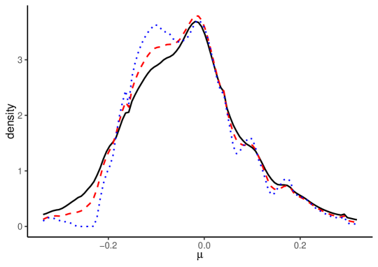
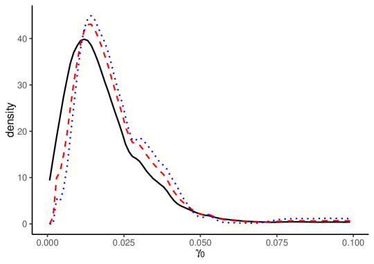
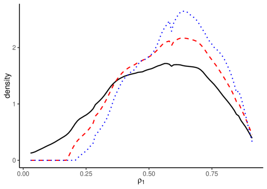
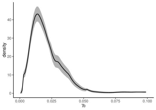
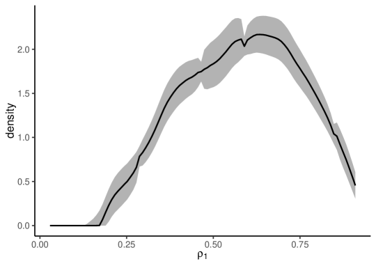
The estimation results with and without bias correction show that the LOP deviation dynamics are significantly heterogeneous across items. The density estimates without bias correction for are similar to those with bias correction. The results for also show that the mode of the heterogeneous long-run LOP deviations is close to zero, with a nearly symmetric, unimodal distribution. In contrast, the estimates without bias correction for and are very different from the bias-corrected estimates. The bias-corrected estimates for demonstrate larger variances for the LOP deviation dynamics, while the bias-corrected estimates for show more persistent dynamics with a more left-skewed distribution. These results suggest the severe impact of the incidental parameter biases, which highlights the importance of bias correction methods.
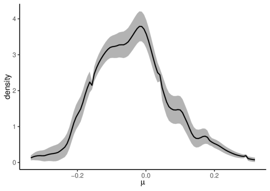
Figure 2 depicts 95% point-wise confidence bands based on the HPJ estimates. The confidence bands are narrow, implying that our HPJ estimates seem to be precise and reliable.
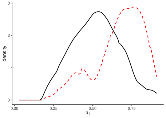
Figure 3 illustrates the HPJ estimates of , , and for goods and services separately. The solid black lines are the HPJ estimates for goods, and the dashed red lines are those for services. The estimated densities and CDFs show that the heterogeneous properties are significantly different between goods and services. The densities for show that the long-run LOP deviation for goods generally tends to be larger than that for services (in an absolute sense). The estimation results for and show that the LOP deviation for goods tends to be more volatile but less persistent than that for services. These results suggest that goods tend to have more volatile processes with faster adjustment speeds toward the nonnegligible long-run LOP deviation.
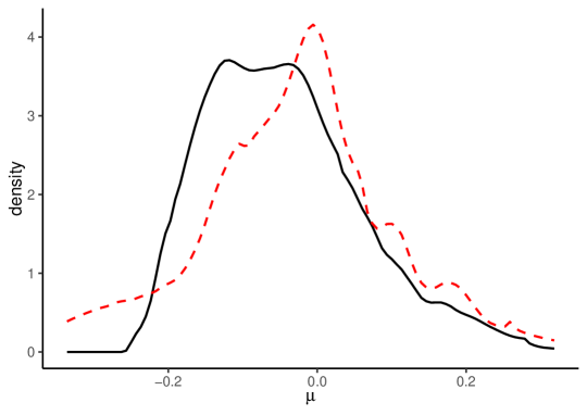
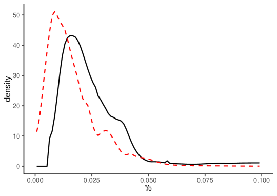
If we seek to examine the degree of heterogeneity of the LOP deviations across items and cities as in Crucini et al. (2015), our model-free results are informative in their own right. There are several possible sources of differences in the degree of heterogeneity, including the differences in trade costs across items (e.g., Anderson and Van Wincoop, 2004) and differences in sale and nonsale prices across goods and services (e.g., Nakamura and Steinsson, 2008). Furthermore, our model-free results also suggest how we should model heterogeneity when implementing structural estimation for price deviations or change. For example, as our procedure demonstrates that the heterogeneous properties of goods and services differ, we should model unobserved heterogeneity differently for goods and services.
5 Conclusion
This paper presented nonparametric kernel-smoothing estimation to examine the degree of heterogeneity in panel data. The kernel density and CDF estimators are consistent and asymptotically normal under the relative magnitude conditions on the cross-sectional size , time-series length , and bandwidth . Because of the presence of incidental parameter bias and nonlinearity biases, the relative magnitude conditions vary in the order of the expansions. Via infinite-order expansions, we derived the relative magnitude conditions that are suitable for microeconometric applications. We discussed the split-panel jackknife to correct biases, the construction of CIs, and the selection of bandwidth. We also illustrated our procedure based on an application on price deviations.
Acknowledgments
The authors greatly appreciate the assistance of Mototsugu Shintani in providing the price panel data. The authors would also like to thank Stephane Bonhomme, Kazuhiko Hayakawa, Koen Jochmans, Shin Kanaya, Hiroyuki Kasahara, Yoonseok Lee, Oliver Linton, Jun Ma, Yukitoshi Matsushita, Martin Weidner, Yohei Yamamoto, Yu Zhu and the participants of many conferences for helpful discussions and comments. Sebastian Calonico kindly helped us better understand the use of the nprobust package. All remaining errors are our own. Part of this research was conducted while Okui was at Vrije Universiteit Amsterdam, Kyoto University, and NYU Shanghai and while Yanagi was at Hitotsubashi University. This work was supported by the New Faculty Startup Fund from Seoul National University, JSPS KAKENHI Grant Numbers JP25780151, JP25285067, JP15H03329, JP16K03598, JP15H06214, and JP17K13715.
References
- Ackerberg et al. (2007) D. Ackerberg, C. L. Benkard, S. Berry, and A. Pakes. Econometric tools for analyzing market outcomes. In J. J. Heckman and E. E. Leamer, editors, Handbook of Econometrics, volume 6, chapter 63, pages 4171–4276. Elsevier, 2007.
- Anderson and Van Wincoop (2004) J. E. Anderson and E. Van Wincoop. Trade costs. Journal of Economic Literature, 42(3):691–751, 2004.
- Arellano and Bonhomme (2012) M. Arellano and S. Bonhomme. Identifying distributional characteristics in random coefficients panel data models. Review of Economic Studies, 79:987–1020, 2012.
- Calonico et al. (2018a) S. Calonico, M. D. Cattaneo, and M. H. Farrell. On the effect of bias estimation on coverage accuracy in nonparametric inference. Journal of the American Statistical Association, 113(522):767–779, 2018a.
- Calonico et al. (2018b) S. Calonico, M. D. Cattaneo, and M. H. Farrell. nprobust: Nonparametric Robust Estimation and Inference Methods using Local Polynomial Regression and Kernel Density Estimation, 2018b. URL https://CRAN.R-project.org/package=nprobust. R package version 0.1.3.
- Crucini et al. (2015) M. J. Crucini, M. Shintani, and T. Tsuruga. Noisy information, distance and law of one price dynamics across us cities. Journal of Monetary Economics, 74:52–66, 2015.
- Dhaene and Jochmans (2015) G. Dhaene and K. Jochmans. Split-panel jackknife estimation of fixed effects models. Review of Economic Studies, 82:991–1030, 2015.
- Engel and Rogers (2001) C. Engel and J. H. Rogers. Deviations from purchasing power parity: causes and welfare costs. Journal of International Economics, 55(1):29–57, 2001.
- Fernández-Val and Lee (2013) I. Fernández-Val and J. Lee. Panel data models with nonadditive unobserved heterogeneity: Estimation and inference. Quantitative Economics, 4:453–481, 2013.
- Galvao and Kato (2014) A. F. Galvao and K. Kato. Estimation and inference for linear panel data models under misspecification when both and are large. Journal of Business and Economic Statistics, 32(2):285–309, 2014.
- Guerre et al. (2000) E. Guerre, I. Perrigne, and Q. Vuong. Optimal nonparametric estimation of first-price auctions. Econometrica, 68(3):525–574, 2000.
- Hall and Horowitz (2013) P. Hall and J. Horowitz. A simple bootstrap method for constructing nonparametric confidence bands for functions. The Annals of Statistics, 41(4):1892–1921, 2013.
- Horowitz and Markatou (1996) J. L. Horowitz and M. Markatou. Semiparametric estimation of regression models for panel data. Review of Economic Studies, 63(1):145–168, 1996.
- Hsiao et al. (1999) C. Hsiao, M. H. Pesaran, and A. K. Tahmiscioglu. Bayes estimation of short-run coefficients in dynamic panel data models. In K. L. C. Hsiao, L.F. Lee and M. Pesaran, editors, Analysis of Panels and Limited Dependent Variables Models, pages 268–296. Cambridge University press, 1999.
- Jochmans and Weidner (2019) K. Jochmans and M. Weidner. Inference on a distribution from noisy draws. Cambridge Working Paper in Economics 19/46, 2019.
- Kasahara et al. (2017) H. Kasahara, P. Schrimpf, and M. Suzuki. Identification and estimation of production function with unobserved heterogeneity. mimeo, 2017.
- Klenow and Malin (2010) P. J. Klenow and B. A. Malin. Microeconomic evidence on price-setting. Handbook of Monetary Economics, 3:231–284, 2010.
- Lee et al. (2018) Y.-J. Lee, R. Okui, and M. Shintani. Asymptotic inference for dynamic panel estimators of infinite order autoregressive processes. Journal of Econometrics, 204:147–158, 2018.
- Li and Racine (2007) Q. Li and J. S. Racine. Nonparametric Econometrics: Theory and Practice. Princeton University Press, 2007.
- Ma et al. (2019) J. Ma, V. Marmer, and A. Shneyerov. Inference for first-price auctions with Guerre, Perrigne, and Vuong’s estimator. forthcoming in the Journal of Econometrics, 2019.
- Mavroeidis et al. (2015) S. Mavroeidis, Y. Sasaki, and I. Welch. Estimation of heterogenous autoregressive parameters using short panel data. Journal of Econometrics, 188:219–235, 2015.
- Nakamura and Steinsson (2008) E. Nakamura and J. Steinsson. Five facts about prices: A reevaluation of menu cost models. The Quarterly Journal of Economics, 123(4):1415–1464, 2008.
- Neyman and Scott (1948) J. Neyman and E. L. Scott. Consistent estimates based on partially consistent observations. Econometrica, 16:1–32, 1948.
- Nickell (1981) S. Nickell. Biases in dynamic models with fixed effects. Econometrica, 49(6):1417–1426, 1981.
- Okui (2008) R. Okui. Panel AR(1) estimators under misspecification. Economics Letters, 101:210–213, 2008.
- Okui (2011) R. Okui. Asymptotically unbiased estimation of autocovariances and autocorrelations for panel data with incidental trends. Economics Letters, 112:49–52, 2011.
- Okui (2014) R. Okui. Asymptotically unbiased estimation of autocovariances and autocorrelations with panel data in the presence of individual and time effects. Journal of Time Series Econometrics, 6(2):129–181, 2014.
- Okui and Yanagi (2019) R. Okui and T. Yanagi. Panel data analysis with heterogeneous dynamics. forthcoming in Journal of Econometrics, 2019.
- Pagan and Ullah (1999) A. Pagan and A. Ullah. Nonparametric Econometrics. Cambridge University Press, 1999.
- Parsley and Wei (1996) D. C. Parsley and S.-J. Wei. Convergence to the law of one price without trade barriers or currency fluctuations. Quarterly Journal of Economics, 111(4):1211–1236, 1996.
- Parsley and Wei (2001) D. C. Parsley and S.-J. Wei. Explaining the border effect: the role of exchange rate variability, shipping costs, and geography. Journal of International Economics, 55(1):87–105, 2001.
- Pesaran and Smith (1995) M. H. Pesaran and R. Smith. Estimating long-run relationships from dynamic heterogeneous panels. Journal of Econometrics, 68(1):79–113, 1995.
- Pesaran et al. (1999) M. H. Pesaran, Y. Shin, and R. P. Smith. Pooled mean group estimation of dynamic heterogeneous panels. Journal of the American Statistical Association, 94(446):621–634, 1999.
- Quenouille (1949) M. H. Quenouille. Approximate tests of correlation in time-series 3. In Mathematical Proceedings of the Cambridge Philosophical Society, volume 45-03, pages 483–484. Cambridge Univ Press, 1949.
- Quenouille (1956) M. H. Quenouille. Notes on bias in estimation. Biometrika, 43(3 and 4):353–360, 1956.
- Roca and Puga (2017) J. D. L. Roca and D. Puga. Learning by working in big cities. Review of Economic Studies, 84(1):106–142, 2017.
- Yazgan and Yilmazkuday (2011) M. E. Yazgan and H. Yilmazkuday. Price-level convergence: New evidence from U.S. cities. Economics Letters, 110(2):76–78, 2011.
Supplementary Appendix of “Kernel Estimation for Panel Data with Heterogeneous Dynamics”
Ryo Okui and Takahide Yanagi
May, 2019
This supplementary appendix contains technical discussions omitted from the main text and Monte Carlo simulation results. Appendix A presents the proofs of the theorems in the main body of the paper. Appendix B presents the technical lemmas used in the proofs of the theorems. Appendices C and D present the technical discussions on the validity of the infinite-order expansions in Theorem 1. Appendix E presents the simulation results.
Appendix A Appendix: Proofs of the theorems
This appendix collects the proofs of the theorems. In the following, we denote a generic positive constant by .
A.1 Proof of Theorem 1
The density of .
We evaluate each term in the following Taylor expansion:
| (A.1) | ||||
| (A.2) | ||||
| (A.3) |
For (A.1), we use the standard results for the kernel density estimation. Lemma 7 under Assumptions 1, 5, and 6 shows that as and with . Furthermore, Lemma 7 also shows that:
as and with and .
For (A.2), the mean is zero by the law of iterated expectations, because and . The variance is:
by Lemmas 1 and 6. Therefore, (A.2) is by Markov inequality.
For the term in (A.3), the mean is:
by the law of iterated expectations and Lemma 6 with the definition of
The variance is:
by Lemmas 1 and 6. Thus, it holds that:
Consequently, we obtain the desired result for by Slutsky’s theorem.
The density of .
We evaluate each term in the following Taylor expansion:
| (A.4) | ||||
| (A.5) | ||||
| (A.6) |
For (A.4), the consistency and asymptotic normality of the term are established by the same argument as for the density of .
For (A.5), we have the following equation based on the expansion for :
| (A.7) | ||||
| (A.8) | ||||
| (A.9) | ||||
| (A.10) |
For (A.7), the mean is zero by the law of iterated expectations given . The variance is:
by Lemmas 3 and 6. Thus, (A.7) is . For (A.8), denoting , the mean is expanded as:
by the law of iterated expectations, Lemma 6, and with the definition of:
The variance is:
by the Cauchy–Schwarz inequality and Lemmas 1 and 6. Thus, (A.8) is . For (A.9), the triangle inequality and the Cauchy–Schwarz inequality lead to:
by Lemmas 1 and 6. Thus, (A.9) is . In the same manner, we can show that (A.10) is also . These results mean that (A.5) is .
For (A.6), it is easy to see that:
by the same procedures to show the order of the terms in (A.5). The mean of the term is:
by the law of iterated expectations and Lemma 6 with the definition of
The variance of the term is:
by Lemmas 3 and 6. Thus, it holds that:
Consequently, we obtain the desired result for by Slutsky’s theorem.
The density of .
We regard as a function of two variables . Taylor’s theorem for multivariate functions leads to:
| (A.11) | ||||
| (A.12) | ||||
| (A.13) |
We evaluate each term below.
For (A.11), the consistency and asymptotic normality of the term are established by the same argument as for the density of .
(A.12) contains two terms. Of these, we consider only , because the other term can be evaluated by the same argument. However, this term is analogous to that in (A.5), so it can be evaluated by the same argument. This means that (A.12) can be written as for a nonrandom .
For (A.13), we evaluate the mean of the term:
which contains terms. Among these, we consider only , as the other terms can be evaluated in the same manner. However, this term is analogous to that in (A.6), so it can be evaluated by the same argument. This means that (A.13) can be written as:
for a nonrandom .
Consequently, we have the desired result for by Slutsky’s theorem. ∎
A.2 Proof of Theorem 2
We show the proof for the density estimator of only. Those of and are the same. The proof of Theorem 1 has shown that:
This result implies that the estimators based on the half-panel data are:
for . As a result, the HPJ bias-corrected estimator satisfies:
Therefore, the same argument as for the term in (A.4) leads to the desired result. ∎
A.3 Proof of Theorem 3
The CDF of .
We evaluate each term in the following Taylor expansion:
| (A.14) | ||||
| (A.15) | ||||
| (A.16) | ||||
| (A.17) |
For the term in (A.14), Lemma 8 under Assumptions 1, 5, and 8 shows that:
as and . Moreover, Lemma 8 also shows that:
as and with .
For (A.15), the mean is zero given and . The variance is:
For (A.16), we define . The mean is:
by the law of iterated expectations, Lemma 6, and with the definition of
The variance is:
For the term in (A.17), the mean is:
by the law of iterated expectations and Lemmas 1 and 6 with the definition of
The variance is:
by Lemmas 2 and 6. Thus, (A.17) can be written as:
Consequently, we obtain the desired result for by Slutsky’s theorem.
The CDF of .
We evaluate each term in the following Taylor expansion:
| (A.18) | ||||
| (A.19) | ||||
| (A.20) | ||||
| (A.21) |
For (A.18), consistency and asymptotic normality are established by the same arguments as for the CDF of .
For (A.19), we have the following equation by the expansion for :
| (A.22) | ||||
| (A.23) | ||||
| (A.24) | ||||
| (A.25) |
For the term in (A.22), the mean is zero and the variance is:
by Lemmas 3 and 6. Thus, (A.22) is . For (A.23), the mean is:
by the law of iterated expectations and Lemma 6 with the definition of
The variance is:
by Lemmas 1 and 6. Thus, (A.23) is . For (A.24), the absolute mean is:
by Lemmas 1 and 6. Thus, (A.24) is . For (A.25), we can show that it is by the same argument. Thus, (A.19) is .
For (A.20), it is easy to see that:
by similar procedures, to show the orders of (A.22), (A.23), (A.24), and (A.25). Introducing the shorthand notation , the mean of the term is:
by Lemma 6 and with the definition of
The variance of the term is:
For (A.21), it is easy to see that:
by the same argument as for (A.20). The mean of the term is:
by Lemma 6 with the definition of
The variance is:
by Lemmas 4 and 6. Thus, (A.21) can be written as:
Consequently, we obtain the desired result for by Slutsky’s theorem.
The CDF of .
We regard as a function of two variables . Taylor’s theorem for multivariate functions leads to:
| (A.26) | ||||
| (A.27) | ||||
| (A.28) | ||||
| (A.29) |
For (A.26), the consistency and asymptotic normality of the term are established by the same argument as for the CDF of .
(A.27) contains two terms. Of these, we focus only on , as the other term can be evaluated in the same manner. However, this term is analogous to that in (A.19), so it can be evaluated by the same argument. This means that (A.27) can be written as for a nonrandom .
(A.28) contains three terms. Of these, we focus only on , as the other terms can be evaluated in the same manner. However, this term is analogous to that in (A.20), so it can be evaluated by the same argument. This means that (A.28) is also for a nonrandom .
For (A.29), we evaluate the mean of the term
which contains terms. Of these terms, we consider only:
as the other terms can be evaluated in the same manner. However, this term is analogous to that in (A.21), so we can evaluate it using the same argument. This means that (A.29) can be written as:
for a nonrandom .
Consequently, we have the desired result for by Slutsky’s theorem. ∎
Appendix B Appendix: Lemmas
This appendix contains the technical lemmas used to demonstrate the theorems in the main body.
We first present the lemmas for which the proofs are given in Okui and Yanagi (2019).
Lemma 1.
Lemma 2.
Lemma 3.
Lemma 4.
Lemma 5.
We repeatedly use the following lemmas to prove our theorems. The proofs are similar to those in Pagan and Ullah (1999) and Li and Racine (2007), and are omitted.
Lemma 6.
Consider a continuous random variable , a random vector , and an interior point . Suppose that a function satisfies , , and , and that and the density are twice boundedly continuously differentiable at . It holds that
where .
Note that the above result implies that, if we set (constant):
Suppose that is a random sample of a continuous random variable . We denote the density and CDF of by and , respectively.
Lemma 7.
Let be the kernel density estimator. Let be a fixed interior point in the support of . Suppose that the kernel function is symmetric and satisfies , , , and , and that is bounded away from zero and three-times boundedly continuously differentiable near . When and with , it holds that and . Moreover, when and , it holds that .
Lemma 8.
Let be the kernel CDF estimator. Let be a fixed interior point in the support of . Let be the derivative. Suppose that is symmetric and satisfies , , , and , and that is three-times boundedly continuously differentiable near . When and , then and . Moreover, when also holds, it holds that .
Appendix C Appendix: The validity of the infinite-order Taylor expansion
This appendix discusses the validity of the infinite-order Taylor expansion for the density estimation in Theorem 1. The discussion for the expansion of the CDF estimation in Theorem 3 is similar.
The infinite-order Taylor expansion of is:
It holds if the remainder term of the finite-order Taylor expansion converges to zero as the order of the expansion increases. We show that it is the case with probability approaching one. The remainder term is given by:
where is between and . It is sufficient to argue that it converges to zero, as , with probability approaching one. We observe that:
| (A.30) |
We argue that the term in the first parenthesis of (A.30) converges to zero, as , with probability approaching one. Note that the convergence holds when . For this, we observe that for any fixed and positive integer :
| (A.31) |
by Assumption 1, Markov’s inequality, and Lemma 2, 4, or 5 with fixed . The probability on the left-hand side of (A.31) thus converges to one if . Based on the binomial theorem, we observe that:
As a result, the probability on the left-hand side of (A.31) converges to one if for sufficiently large as and . By taking , we obtain the desired result. We note that the condition is significantly weaker than the relative magnitudes condition in Theorem 1. Hence, the term in the first parenthesis of (A.30) converges to zero, as , with probability approaching one.
In a similar manner, we can observe that the term in the second parenthesis of (A.30) converges to zero with probability approaching one under regularity conditions.
Therefore, the infinite-order Taylor expansion in Theorem 1 holds under regularity conditions.
Appendix D Appendix: The infinite series of the asymptotic biases
This appendix discusses the conditions under which the infinite series of the asymptotic biases is well defined (i.e., summable and convergent). We focus on the density estimator for only, because the discussions for the other estimators are similar.
To examine the series of the asymptotic biases, we focus on the nonlinearity biases of the density estimator . Let . For the nonlinearity bias in (A.3) of the proof of the density estimation, we observe that:
by the law of iterated expectations, the change of variables, and Taylor’s theorem with located between and . The equation for any odd is equal to:
because of the symmetry of . On the contrary, the equation for any even is equal to:
We focus on the summability of the series of the biases for odd only, because the discussion for even is the same. The partial sum of the series of the biases for odd can be written as:
where we define the variables and .
We examine the series of only. The discussion for is the same. The ratio test means that the series is summable and convergent if . We observe that:
for any . It converges to zero as if over and if . The former is a regularity condition, and we can simply assume it. The latter is also a regularity condition, and we can easily show its validity by assuming that is the Gaussian kernel function. Hence, the condition for the ratio test is satisfied, implying that the series is summable and convergent.
The above discussions imply that the infinite series of the asymptotic biases is well defined under regularity conditions.
Appendix E Appendix: Monte Carlo simulations
This section presents the results of the Monte Carlo simulations. We here focus on the density estimation only. The number of simulation replications is 5,000.
Design.
We generate the data using the AR(1) process where , , and . Note that this design satisfies , , and . We generate the unit-specific random variables , , and . We consider and .
Estimators.
We estimate the densities of , , and at their 20%, 40%, 60%, and 80% quantiles based on four estimators. The first is the naive estimator (NE) without split-panel jackknife bias correction. The second and third are the HPJ and TOJ estimators. The fourth is the infeasible estimator (IE) based on the true , , and . For all estimators, we use the Epanechnikov kernel and the coverage error optimal bandwidth in Calonico et al. (2018a).
Results.
Tables 1, 2, and 3 present the simulation results for the densities of , , and , respectively. The tables report the true values of the parameters and the bias and standard deviation (std) of each estimator. They also report the coverage probability (cp) of the 95% CI computed by the RBC procedure based on each estimator. Table 4 also describes the mean and the standard deviation of the selected bandwidths for NE and IE. Note that we use the same bandwidth for HPJ and TOJ as NE as discussed in the main body.
The NE exhibits large biases, especially with small . In particular, the biases of the density for and are crucial because of the incidental parameter biases. As a result, the coverage probabilities of the NE are much smaller than 0.95. The performance of the NE improves as grows, but it is unsatisfactory for several parameters even when . These results highlight the importance of bias correction even with relatively large .
The performances of the HPJ and TOJ are significantly better than the NE. The HPJ and TOJ operate well especially when the NE exhibits large biases. The TOJ outperforms the HPJ when the HPJ exhibits relatively large biases, as a result of relatively large higher-order nonlinearity biases. Furthermore, for several parameters, the TOJ operates as well as the IE in terms of bias reduction and coverage probability. Note that the TOJ may inflate the estimation variability, especially when is small, but such cost is inevitable when our goal is to conduct unbiased inferences.
These simulation results demonstrate the severity of the incidental parameter biases and the nonlinearity biases and the success of the split-panel jackknife and the RBC inference. We thus recommend the RBC inference based on the split-panel jackknife bias-corrected estimation.
| NE | HPJ | TOJ | IE | ||||||||||||||||
|---|---|---|---|---|---|---|---|---|---|---|---|---|---|---|---|---|---|---|---|
| true | bias | std | cp | bias | std | cp | bias | std | cp | bias | std | cp | |||||||
| at ’s 20%Q | |||||||||||||||||||
| at ’s 40%Q | |||||||||||||||||||
| at ’s 60%Q | |||||||||||||||||||
| at ’s 80%Q | |||||||||||||||||||
| NE | IE | NE | IE | NE | IE | |||||||||||||||
|---|---|---|---|---|---|---|---|---|---|---|---|---|---|---|---|---|---|---|---|---|
| mean | std | mean | std | mean | std | mean | std | mean | std | mean | std | |||||||||
| at 20% Q | ||||||||||||||||||||
| at 40% Q | ||||||||||||||||||||
| at 60% Q | ||||||||||||||||||||
| at 80% Q | ||||||||||||||||||||