Kernel Packet: An Exact and Scalable Algorithm for Gaussian Process Regression with Matérn Correlations
Abstract
We develop an exact and scalable algorithm for one-dimensional Gaussian process regression with Matérn correlations whose smoothness parameter is a half-integer. The proposed algorithm only requires operations and storage. This leads to a linear-cost solver since is chosen to be fixed and usually very small in most applications. The proposed method can be applied to multi-dimensional problems if a full grid or a sparse grid design is used. The proposed method is based on a novel theory for Matérn correlation functions. We find that a suitable rearrangement of these correlation functions can produce a compactly supported function, called a “kernel packet”. Using a set of kernel packets as basis functions leads to a sparse representation of the covariance matrix that results in the proposed algorithm. Simulation studies show that the proposed algorithm, when applicable, is significantly superior to the existing alternatives in both the computational time and predictive accuracy.
Keywords: Computer experiments, Kriging, Uncertainty quantification, Compactly supported functions, Sparse matrices
1 Introduction
Gaussian process (GP) regression is a powerful function reconstruction tool. It has been widely used in computer experiments (Santner et al., 2003; Gramacy, 2020), spatial statistics (Cressie, 2015), supervised learning (Rasmussen, 2006), reinforcement learning (Deisenroth et al., 2013), probabilistic numerics (Hennig et al., 2015) and Bayesian optimization (Srinivas et al., 2009). GP regression models are flexible to fit a variety of functions, and they also enable uncertainty quantification for prediction by providing predictive distributions. With these appealing features, GP regression has become the primary surrogate model for computer experiments since popularized by Sacks et al. (1989). Despite these advantages, Gaussian process regression has its drawbacks. A major one is its computational complexity. Training a GP model requires furnishing matrix inverses and determinants. With training points, each of these matrix manipulations takes operations (referred to as “time” thereafter, assuming for simplicity that no parallel computing is enforced) if a direct method, such as the Cholesky decomposition, is applied. Besides, the computation for model training may also be hindered by the storage requirement (Gramacy, 2020) to store the covariance matrix.
Tremendous efforts have been made in the literature to address the computational challenges of GP regression. Recent advances in scalable GP regression include random Fourier features (Rahimi and Recht, 2007), Nyström Approximation (also known as inducing points) (Smola and Schölkopf, 2000; Williams and Seeger, 2001; Titsias, 2009; Bui et al., 2017; Katzfuss, 2017; Chen and Stein, 2021), structured kernel interpolation Wilson and Nickisch (2015), etc. These methods are based on different types of approximation of GPs, i.e., the efficiency is gained at the cost of its accuracy. In contrast, the main objective of this work is to propose a novel scalable approach that does not need an approximation.
In this work, we focus on the use of GP regression in the context of computer experiments. In these studies, the training data are acquired through an experiment, in which the input points can be chosen. Such a choice is called a design of the experiment. It is well known that a suitably chosen design can largely simplify the computation. Here we consider the “tensor-space” techniques in terms of using a product correlation function and a full grid or a sparse grid (Plumlee, 2014) design. The tensor-space techniques can reduce a multivariate GP regression problem to several univariate problems. It is worth noting that, in some applications besides computer experiments, even if the input sites are not controllable, the data are naturally observed on full grids, e.g., the remote sensing data in geoscience applications (Bazi and Melgani, 2009). In these scenarios, the tensor-space techniques are also applicable.
Having the tensor-space techniques, the final hard nut to crack is the one-dimensional GP regression problem. We assume that the one-dimensional input data are already ordered throughout this work. This assumption is reasonable in computer experiment applications since the design points are chosen at our will. In other applications where we do not have ordered data in the first place, it takes only time to sort them.
This work presents a mathematically exact algorithm to make conditional inference for one-dimensional GP regression with time and space complexity both linear in . This algorithm is specialized for Matérn correlations with smoothness being a half-integer (see Section 1.1 for the definition.) Matérn correlations are commonly used in practice (Stein, 1999; Santner et al., 2003; Gramacy, 2020). In most applications, is chosen to be small, e.g., or , for the sake of a higher model flexibility. The proposed algorithm enjoys the following important features.
-
•
Given the hyper-parameters of the GP, the proposed algorithm is mathematically exact, i.e., all numerical error is attributed to the roundoff error given by the machine precision.
-
•
There is no restriction for the one-dimensional input points. But if the points are equally spaced, the computational time can be further reduced.
-
•
It takes only time to compute the matrix inversion and the determinant. For equally spaced designs, this time is further reduced to .
-
•
After the above pre-processing time, it takes only or even time to make a new prediction (i.e., evaluate the conditional mean) at an untried point.
-
•
The storage requirement is only .
The remainder of this article is organized as follows. We will review the general idea of GP regression and some existing algorithms in Sections 1.1 and 1.2, respectively. The mathematical theory behind the proposed algorithm is introduced in Section 2. In Section 3, we propose the main algorithm. Numerical studies are given in Section 4. In Section 5, we briefly discuss some possible extensions of the proposed method. Concluding remarks are made in Section 6. Appendices A and B contain the required mathematical tools and our technical proofs, respectively.
1.1 A review on GP Regression
Let denote a stationary GP prior on with mean function , variance , and correlation function . The correlation function is also referred to as a “kernel function” in the language of applied math or machine learning (Rasmussen, 2006). When , there are two types of popular correlation functions. The first type is the Matérn family (Stein, 1999):
| (1) |
for any , where is the smoothness parameter, is the scale and is the modified Bessel function of the second kind. The smoothness parameter governs the smoothness of the GP (Santner et al., 2003; Stein, 1999); the scale parameter determines the spread of the correlation (Rasmussen, 2006). Matérn correlation functions are widely used because of its great flexibility. The second type is the Gaussian family:
| (2) |
for any . A Gaussian kernel function is the limit of a sequence of Matérn kernels with the smoothness parameter tending to infinity. The sample paths generated by GP with Gaussian correlation function are infinitely differentiable.
For multi-dimensional problems, a typical choice of the correlation structure is the separable or product correlation:
| (3) |
for any , where is a one-dimensional Matérn or Gaussian correlation function for each . This assumption ensures that the GP lives in a tensor space, and is key to the “tensor-space” techniques, which reduces the multi-dimensional problems to one-dimensional ones.
Suppose that we have observed on distinct points . The aim of GP regression is to predict the output at an untried input by computing the distribution of conditional on , which is a normal distribution with the following conditional mean and variance (Santner et al., 2003; Banerjee et al., 2014):
| (4) | |||
| (5) |
where is the variance, , and .
In GP regression, the mean function is usually parametrized as a linear form for some unknown coefficient vector and known regression functions . To improve the predictive performance of GP regression, the coefficient vector , variance and scales associated to each one-dimensional correlation function are usually estimated via maximum likelihood (Jones et al., 1998). The log-likelihood function given the data is:
| (6) |
where denotes the determinant of the correlation matrix and is the matrix whose entry is . The Maximum Likelihood Estimator (MLE) is then defined as the maximimizer of the log-likelihood function: .
In both GP regression and parameter estimation, the computation can become unstable or even intractable because it involves the pursuit of the inversion and the determinant of the correlation matrix . Each task takes time if a direct method, such as the Cholesky decomposition, is applied, which is a fundamental computational challenge for GP regression.
1.2 Comparisons with Existing Methods
When applicable, as a specialized algorithm, the proposed method is significantly superior to the existing alternatives. In this section, we compare the proposed method with a few popular existing approaches for large-scale GP regression. It is worth noting that, the fundamental mathematical theory for the proposed method differs from that of any of the existing methods. A summary of the comparisons is presented in Table 1.
| Method | Kernels | Design | Time | Storage | Accuracy |
| Proposed Method | Matérn-, | Arbitrary | Exact | ||
| Stationary | Equally | Depending on the | |||
| Toeplitz Methods | Kernels | Spaced | number of iterations | ||
| Local Approximate GP | |||||
| (with nearest neighbors) | Arbitrary | Arbitrary | Unknown | ||
| Random Fourier Features | Matérn- | ||||
| (with random features) | Gaussian | Arbitrary | |||
| Nyström Approximation | Matérn- | Matérn: | |||
| (with inducing points) | Gaussian | Arbitrary | Gaussian: |
Toeplitz methods: Toeplitz methods (Wood and Chan, 1994) work for stationary GPs with equally spaced design points. These methods leverage the Toeplitz structure of the covariance matrices under this setting. To make a prediction in terms of solving (4) and (5), there are two approaches. The first is to solve the Toeplitz system exactly, using, for example, the Levinson algorithm (Zhang et al., 2005). This takes time. A more commonly used approach is based on a conjugate gradient algorithm (Atkinson, 2008) to solve the matrix inversion problems in (4) and (5). Each step takes time. For the sake of rapid computation, the number of iterations is chosen to be small. But then the method becomes inexact. Moreover, the conjugate gradient algorithm is unable to find the determinant in (6) (Wilson and Nickisch, 2015). Thus one has to resort to the exact algorithm to compute the likelihood value, which takes time. Toeplitz methods only works for equally spaced design points. This is a strong restriction for one-dimensional problems. For multi-dimensional problems in a tensor space, having this restriction can also be disturbing, especially under a sparse grid design. Many famous sparse grid designs are not based on equally spaced one-dimensional points, such as the Clenshaw-Curtis sparse grids (Gerstner and Griebel, 1998) or the ones suggested by Plumlee (2014).
Local Approximate Gaussian Processes: Gramacy and Apley (2015) proposed a sequential design scheme that dynamically defines the support of a Gaussian process predictor based on a local subset of the data. The local subset comprises of data points and, consequently, local approximate GP reduces the time and space complexity of GPs regression to and respectively. Local approximate GPs can achieve a decent accuracy level in empirical experiments but theoretical properties of this algorithm are still unknown.
Random Fourier Features: The class of Fourier features methods originates from the work by Rahimi and Recht (2007). These methods essentially use to approximate , where are basis functions constructed based on random samples from the spectral density, i.e., the Fourier transform of the kernel function . This low-rank approximation reduces the time and space complexity of GP regression to and , respectively, with accuracy (Sriperumbudur and Szabo, 2015). Clearly, the price for fast computation of random Fourier features is the loss of its accuracy.
Nyström Approximation: These methods approximate the covariance matrix by an matrix , where are called the inducing points. Similar to random Fourier features, Nyström approximations reduce the time complexity and space complexity of GP regression to and , respectively. There are several approaches to choose the inducing points. Smola and Schölkopf (2000); Williams and Seeger (2001) selected from data points by an orthogonalization procedure. Titsias (2009); Bui et al. (2017) treated as hidden variables and select these inducing points via variational Bayesian inference. Katzfuss (2017); Chen and Stein (2021) further developed the Nyström approximation to construct more precise kernel approximations with multi-resolution structures. For Matérn- kernel with , it is shown in Burt et al. (2019) that the accuracy level of any inducing points method is , which is higher than that of the random Fourier features. It was also shown in Tuo and Wang (2020) that GP regression with Matérn- kernel converges to the underlying true GP at the rate and, hence, the number of inducing points should satisfy to achieve the optimal order of approximation accuracy. In this case, the time and space complexity of Nyström approximations are and , respectively. These are higher than that of the proposed algorithm, not to mention that the latter provides the exact solutions.
Other methods: Using a compactly supported kernel (Gramacy, 2020) can induce a sparse covariance matrix, which can lead to an improvement in matrix manipulations. However, if the support of the kernel remains the same while the design points become dense in a finite interval, the sparsity of the covariance matrix is not high enough to improve the order of magnitude. On the other hand, shrinking the support may substantially change the sample path properties of the GP, and impair the power of prediction. Recently, Loper et al. (2021) proposed a general approximation scheme for one-dimensional GP regression, which results in a linear-time inference method.
2 Theory of Kernel Packet Basis
In this section, we introduce the mathematical theory for the novel approach of inverting the correlation matrix in (4) and (5). Technical proofs of all theorems are deferred to Appendix B.
Direct inverting the matrix in (4) and (5) is time consuming, because is a dense matrix. Note that each entry of is an evaluation of function for some . The matrix is not sparse because the support of is the entire real line. The main idea of this work is to find an exact representation of in terms of sparse matrices. This exact representation is built in terms of a change-of-basis transformation.
In this section, we suppose is a one-dimensional kernel. Consider the linear space . The goal is to find another basis for , denoted as , satisfying the following properties:
-
1.
Almost all of the ’s have compact supports.
-
2.
can be obtained from via a sparse linear transformation, i.e., the matrix defining the linear transform from to is sparse.
Unless otherwise specified, throughout this article we assume that the one-dimensional kernel is a Matérn correlation function as in (1), whose spectral density is proportional to ; see Rasmussen (2006); Tuo and Wu (2016). For notational simplicity, let and the above spectral density is proportional to .
2.1 Definition and Existence of Kernel Packets
In this section we introduce the theory that explains how we can find a compactly supported function in . Clearly, such a function must admit the representation Recall the requirement that the linear transform is sparse, which means that most of the coefficients ’s must be zero. This inspires the following definition.
Definition 1
Given a correlation function and input points , a non-zero function is called a kernel packet (KP) of degree , if it admits the representation and the support of is .
At first sight, it seems to be too optimistic to expect the existence of KPs. But, surprisingly, these functions do exist for one-dimensional Matérn correlation functions with half-integer smoothness. We will show that if the smoothness parameter is a half integer, i.e., , there is a KP of degree given any distinct input points.
For simplicity, we will use to parametrize the Matérn correlation, in other words, for . Let be a vector with . The goal is to find coefficients ’s such that
| (7) |
is a KP. We will first find a necessary condition for ’s, and next we will prove that such a condition is also sufficient. We apply the Paley-Wiener theorem (see Lemma 15 in Appendix A and Stein and Shakarchi (2003)), which states that has a compact support only if the inverse Fourier transform of , denoted as , can be extended to an entire function, i.e., a complex-valued function that is holomorphic on the whole complex plane. Let . Our convention of inverse Fourier transform is . Direct calculations show
Clearly, the analytic continuation of this function (up to a constant) is
and this function can be defined at any . Note that the function has poles at , each with multiplicity . According to Paley-Wiener theorem, we have to make an entire function, which implies that , each with multiplicity as well. This condition leads to a set of equations111This statement is formalized as Lemma 20 in Appendix B.:
for , where denotes the th derivative of . Clearly, there are equations, which can be rewritten as
| (8) |
with and , which is a linear system. All solutions to this system are real-valued vectors because all coefficients are real.
Next we study the property of the linear system (8) and the corresponding . Theorem 2 states that can be uniquely determined by (8) up to a multiplicative constant.
Theorem 2
Another important property of (8) is that its solution is not affected by a shift of . Define .
Theorem 3
The solution space of (8), as a function of , is invariant under a shift transformation for any .
Remark 4
Theorem 3 suggests that we can apply a shift on without affecting the solution space. It is worth noting that, although the solution space does not change theoretically, the condition number of the linear system (8) may change, which may significantly affect the numerical accuracy. In order to enhance the numerical stability in solving (8), we suggest standardizing using transformation such that , i.e., . The same standardization technique will be employed in the proof of Theorem 5.
Theorem 5 confirms that any non-zero is indeed a KP.
In other words, we have the following Corollary 6.
Corollary 6
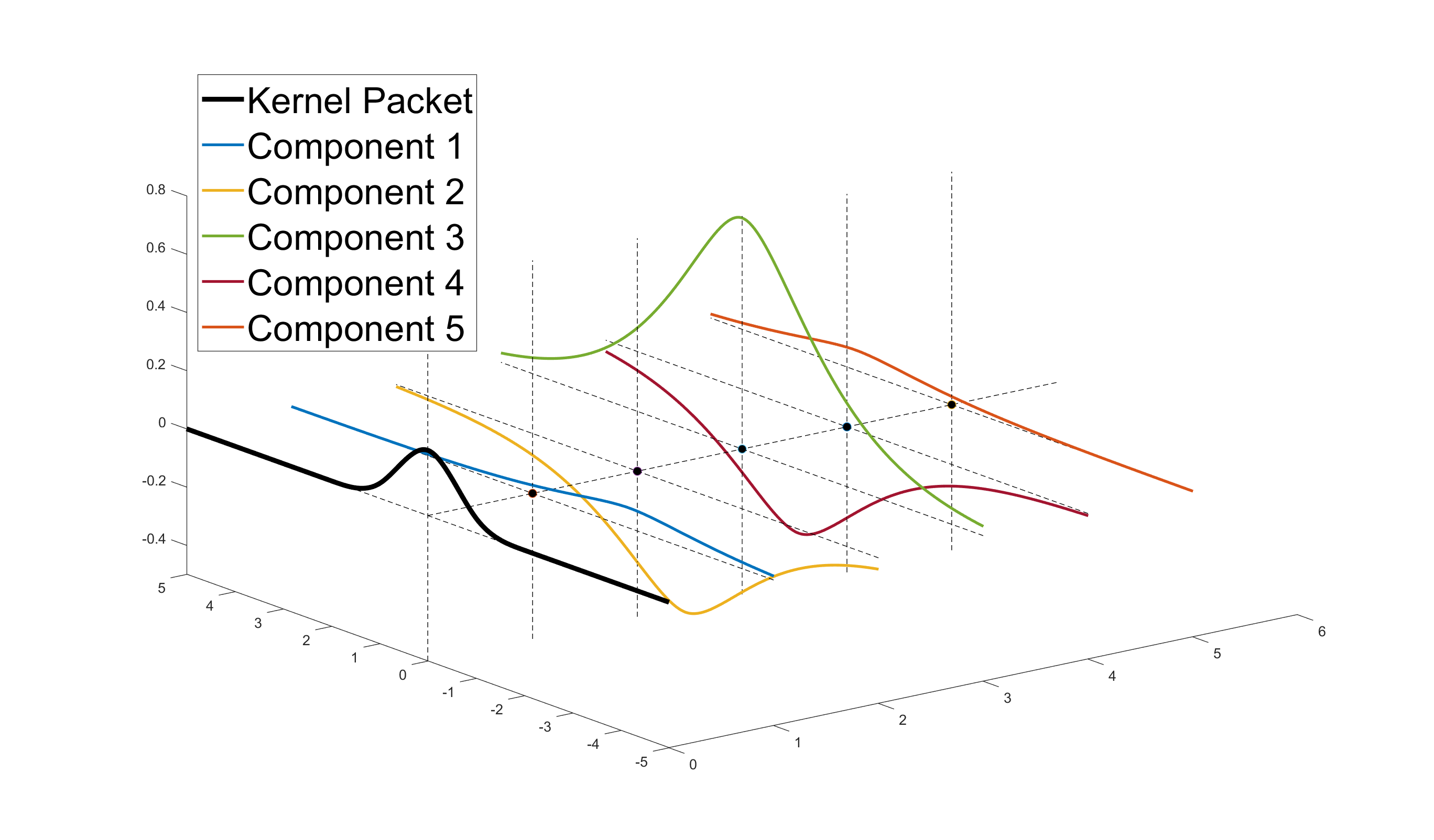
Figure 1 illustrates that the linear combination of components provides a compactly supported KP corresponding to Matérn- correlation function.
It is evident that KPs are highly non-trivial and precious. Their existence relies on the correlation function. Theorem 7 shows that many other correlation function do not admit any KP, and consequently, the proposed algorithm is not applicable to these correlations.
Theorem 7
The following correlation functions do not admit KPs:
-
1.
Any Matérn correlation function whose smoothness parameter is not a half integer.
-
2.
Any Gaussian correlation function.
Theorem 8
Let be a Matérn correlation function with half-integer smoothness . Let be a positive integer with . Then any function of the form does not have a compact support unless for all , and in other words, there does not exist a KP of degree lower than .
2.2 One-sided Kernel Packets
Besides KPs, we need to introduce a set of functions to capture the “boundary effects” of Gaussian process regression. As before, let be a vector with . We consider the functions
| (9) |
with and a non-zero real vector . Then Theorem 8 suggests that in (9) cannot have a compact support. Nevertheless, it is possible that the support of is a half real line. In this case, we cal a one-sided KP. Specifically, we call a right-sided KP if , and we call a left-sided KP if .
First we consider right-sided KPs. We propose to identify ’s by solving
| (10) |
where and the second term of (10) comprises auxiliary equations for the case with . Similar to (8), (10) is an linear system.
The following theorems describes the properties of the linear system (10) and the corresponding . Specifically, Theorem 11 confirms that is indeed a right-sided KP.
Theorem 9
The solution space of (10) is one-dimensional provided that are distinct.
Theorem 10
The solution space of (10), as a function of , is invariant under a shift transformation for any .
2.3 Kernel Packet Basis
Let be the input data, and a Matérn correlation function with a half-integer smoothness. Suppose . We can construct the following functions, as a subset of :
-
1.
, defined as left-sided KPs ,
-
2.
, defined as KPs ,
-
3.
, defined as right-sided KPs .
Note that KPs and one-sided KPs given the input points cannot be uniquely defined. They are unique only up to a non-zero multiplicative factor. Here the choice of these factors are nonessential. The general theory and algorithms in this article will be valid for each specific choice. Now we present Theorem 13, which, together with the fact that the dimension of is , implies that forms a basis for , referred to as the KP basis.
Theorem 13
Let be the input data and the functions are constructed in the above manner. Then the basis functions are linearly independent in .
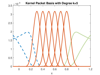
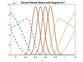
Further, it is straightforward to check via Theorems 5 and 11 that, given any , the vector has at most non-zero entries. As a result, we have constructed a basis for satisfying the two sparse properties mentioned at the beginning of Section 2. Figure 2 illustrates a KP basis corresponding to Matérn- and Matérn- correlation function with input points .
3 Kernel Packet Algorithms
In this section, we will employ the KP bases to develop scalable algorithms for GP regression problems. In Sections 3.1 and 3.2 , we present algorithms for one-dimensional GP regression with noiseless and noisy data, respectively. In section 3.3, we generalize the one-dimensional algorithms to higher dimensions by applying the tensor and sparse grid techniques.
3.1 One-dimensional GP Regression with Noiseless Data
The theory in Section 2 shows that for one-dimensional problems, given ordered and distinct inputs , the correlation matrix admits a sparse representation as
| (12) |
where both and are banded matrices. In (12), the entry of is . In view of the compact supportedness of , is a banded matrix with bandwidth :
The matrix of consists of the coefficients to construct the KPs. In view of the sparse representation, is a banded matrix with bandwidth :
Computing and takes time, because in the construction of each , at most kernel basis functions are needed and the time complexity for solving the coefficients satisfying equation (8), (10) or (11) is . The computational time in this step will dominate that in the next step, which is . However, if the design points are equally spaces, the KP coefficients given by (8) will remain the same for each consecutive data points, so that we only need to compute these values once, and thus the computational time of this step is only . In this case, the computation time in the next step, i.e., , will be dominant, provided that .
Now we solve the GP regression problem, by substituting the identity into (4) and (5) to obtain
| (13) | |||
| (14) |
The key to GP regression now becomes calculating the vector with or . This is equivalent to solving the sparse banded linear system . There exists quite a few sparse linear solvers that can solve this linear system efficiently. For example, the algorithm based on the LU decomposition in Davis (2006) can be applied to solve for in time. MATLAB provides convenient and efficient builtin functions, such as mldivide or decomposition, to solve sparse banded linear system in this form.
It is worth noting that (13) can be executed in the following faster way when we need to evaluate for a many different . First, we compute , which takes time. Next we evaluate for different . As said before, has at most non-zero entries; see Figure 2. If we know which entries are non-zero, the second step takes only time. To find the non-zero entry, a general approach is to use a binary search, which takes time. Sometime, these entries can be found within a constant time. For example, if the design points are equally spaced, there exist explicit expressions for the indices of the non-zero entries; if we need to predict for over a dense mesh (which is a typical task of surrogate modeling), we can use the indices of the non-zero entries for the previous point as an initial guess to find those for the current point.
Similar to the conditional inference, the log-likelihood function (6) can also be computed in time. First, the log-determinant of can be rewritten as , according to identity (12): Because both and are banded matrices, their determinants can be computed in time by sequential methods (Kamgnia and Nguenang, 2014, section 4.1). Second, the same method for the conditional inference can be applied to compute in time.
3.2 One-dimensional GP Regression with Noisy Data
Suppose we observe data , which is a noisy version of . Specifically, , where . In this case, the covariance of the observed noisy responses is . In other words, the covariance matrix is , where is the identity matrix. The posterior predictor at a new point is also normal distributed with the following conditional mean and variance:
| (15) | |||
| (16) |
and the log-likelihood function given data is:
| (17) |
When the input is one dimensional, (15), (16), and (17) can be calculated in as the noiseless case because the covariance matrix admits the following factorization:
| (18) |
By substituting (18) and the identity into (15), (16), and (17), we can obtain:
| (19) | |||
| (20) |
and
| (21) |
We have shown that and are banded matrices with bandwidth and , respectively. Therefore, the matrix is also a banded matrix with bandwidth . Time complexity for computing this sum is . We then can use the algorithms for banded matrices introduced in section 3.1 to compute (19), (20), and (21) in time complexity . Recall that the time complexities for computing and are both . Therefore, in the noisy setting, the total time complexity for computing the posterior and MLE is still , which is the same as the noiseless case.
3.3 Multi-dimensional KP
When data is noiseless, the exact algorithm proposed in Section 3.1 can be used to solve multi-dimensional problems if the input points are full or sparse grids.
A full grid is defined as the Cartesian product of one dimensional point sets: where each denotes any one-dimensional point set. Assuming a separable correlation function (3) comprising one-dimensional Matérn correlation functions with half-integer smoothness, and inputs on a full grid , the covariance vector and covariance matrix decompose into Kronecker products of matrices over each input dimension (Saatçi, 2012; Wilson, 2014):
| (22) | |||
| (23) |
When we compute the vector , the matrix is cancelled as the one dimensional case. Therefore, (4) and (5) can be expressed as
| (24) | |||
| (25) |
and the log-likelihood function (6) becomes
| (26) |
where ’s are the KPs associated to correlation function and point set , is the coefficient matrix for constructing defined in (12), and is the size of , is the size of . We can also note that entries of vector are products of one-dimensional KPs. Therefore, similar to the one-dimensional case, is a vector of compactly supported functions.
In (24)–(26), and can clearly be computed in time. The computation of for is known as Kronecker product least squares (KLS), which has been extensively studied; see, e.g., Graham (2018); Fausett and Fulton (1994). Essentially, the task can be accomplished by sequentially solving problems where the problem is to solve independent banded linear equations with variables. With a banded solver, the total time complexity is .
Although full grid designs result in simple and fast computation of GP regression, their sizes increase exponentially in the dimension. When the dimension is large, another class of grid-based designs called the sparse grids can be practically more useful. Let denote full grids in the form where and is a one-dimensional point set satisfying the nested structure for each . A sparse grid of level is defined as a union of full grids ’s: , where . GP regression on sparse grid designs was first discussed in Plumlee (2014). According to Algorithm 1 in Plumlee (2014), (24) and (25), GP regression on admits the expression
| (27) | |||
| (28) |
where
come from (24) and (25), respectively; and denote the sub-vectors of and on full grid , respectively. Based on Theorem 1 and Algorithm 2 in Plumlee (2014) and (26), and in the log-likehood function (6) can be decomposed as the following linear combinations, respectively:
| (29) | |||
| (30) |
where and denotes the sub-matrix of on full grid .
The above idea of direct computation fails to work for noisy data, because the Kronecker product structure of the covariance matrices breaks down due to the noise. Nonetheless, conjugate gradient methods can be implemented efficiently in the presence of the KP factorization (12). We defer the details to Section 5.
4 Numerical Experiments
We first conduct numerical experiments to assess the performance of the proposed algorithm for grid-based designs on test functions in Section 4.1. Next we employ the proposed method to one-dimensional real datasets in Section 4.2 to further assess its performance.
4.1 Grid-based Designs
4.1.1 Full Grid Designs
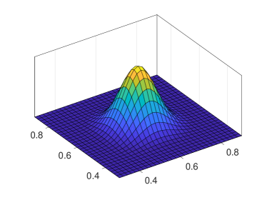
We test our algorithm on the following deterministic function:
Samples of are collected from a level- full grid design: with . The proposed KP algorithm is applied for GP regression using product Matérn correlation function. We choose the same correlation function in each dimension, with , and either or . We will investigate the mean squared error (MSE) and the average computational time over 1000 random test points for each prediction resulting from KP and the following approximation/fast GP regression algorithms with fixed correlation functions.
-
1.
laGP R package 222https://bobby.gramacy.com/r_packages/laGP/. In each experiment, laGP is run under Gaussian covariance family, the only covariance family supported by the package; size of the local subset is set as 100.
-
2.
Inducing Points provided in the GPML tool box (Rasmussen and Nickisch, 2010). The number of inducing points is set as , which is the choice to achieve the optimal approximation power for Matérn- correlation according to Burt et al. (2019). However, if the algorithm crashes due to large sample size, is reduced to a level that the algorithm can run properly. We consider Matérn- and correlations.
-
3.
RFF to approximate Matérn- and Matérn- correlation functions by feature functions , where , are independent and identically distributed (i.i.d.) samples from -distributions with degrees of freedom three and five, respectively, and are i.i.d. samples from the uniform distribution on . If the algorithm crashes due to large sample size, is reduced to a level that the algorithm can run properly.
-
4.
Toeplitz system solver incorporates the one-dimensional Toeplitz method and the Kronercker product technique. We consider Matérn- and correlations. In this experiment we use equally spaced design points, so that the Toeplitz method can work.
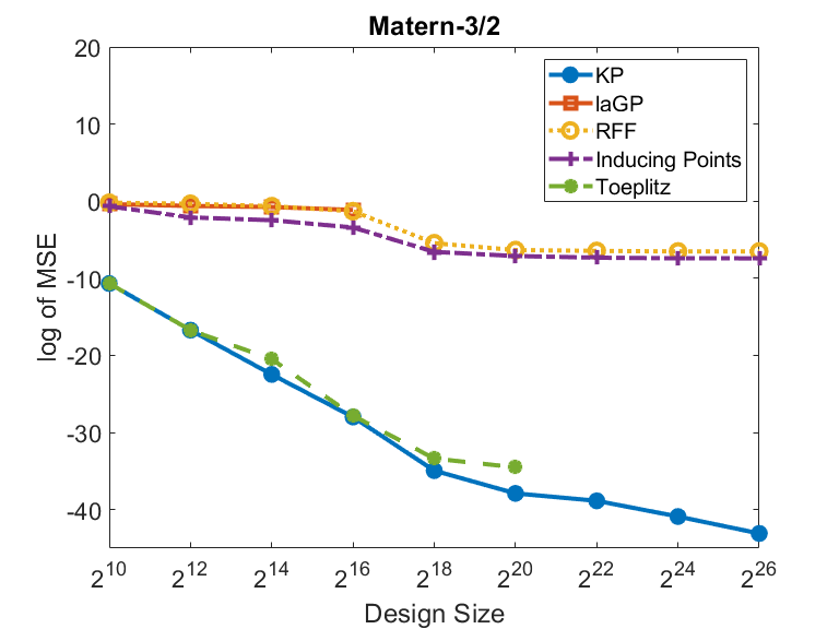
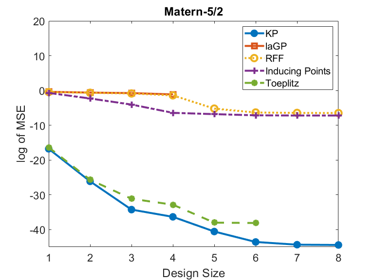
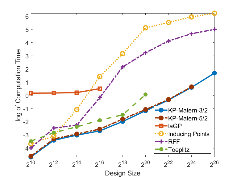
We sample 1000 i.i.d. test points uniformly from for each experimental trial. Figure 4 compares the MSE and the computational time of all algorithms, both under logarithmic scales, for sample sizes , .
The performance curves of some algorithms in Figure 4 are incomplete, because these algorithms fail to work at a certain sample size due to a runtime error, or the prediction MSE ceases to improve. In this case, we stop the subsequent experimental trials with larger sample sizes for these algorithms. Specifically, for sample size larger than , laGP breaks down due to runtime errors. The MSE of Toeplitz ceases to improve at sample size . For sample size larger than , the number of random features for RFF is fixed at and the number of inducing points for inducing points method is fixed at for subsequent trials. Otherwise, both the inducing points method and RFF break down because the approximated covariance matrices are nearly singular. Because of their fixed ’s, the performances of RFF and inducing points method do not have noticeable improvement for sample size larger than . In contrast, KP can run on larger sample sets with sizes up to (more than 67 million) grid points.
It is shown in Figure 4 that KP has the lowest MSE and the fastest computational time in all experimental trials. The inducing points method, laGP and RFF have similar MSE in all experimental trials. The Toeplitz and KP algorithms, which compute the GP regression in exact ways, outperform other approximation methods.
4.1.2 Sparse Grid Designs
We test our algorithm on the Griewank function (Molga and Smutnicki, 2005), defined as
with and respectively. Samples of are collected from a level- sparse grid design . We consider a constant mean and Matérn correlations with and a single scale parameter for all dimensions. We treat mean , variance and scale as unknown variables and use the MLE-predictor. We compare the performance of proposed KP algorithm and the direct method for GP regression on the sparse grids given in Plumlee (2014).
We sample 1000 i.i.d. points uniformly from the input space for each experimental trial. The mean squared error is estimated from these test points. In each trial, the mean squared errors of KP and direct method are in the same order and their differences are within . This is because both methods compute the MLE-predictor in an exact manner, and this also ensures the numerical correctness of the proposed method.
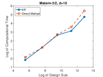
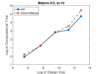
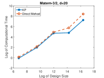
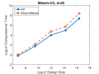
Figure 5 compares the logarithm of the needed computational time to estimate the unknown parameters , and and make predictions on the test points. The proposed KP algorithm is significantly advantageous in the computational time. When there are more than training points, the KP algorithm is at least twice faster than the direct method in each trial.
4.2 Real Datasets
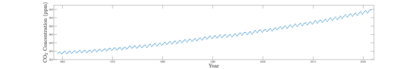
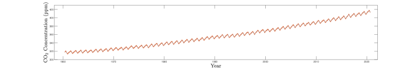
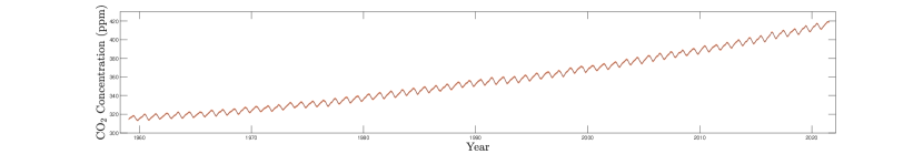
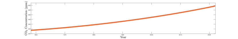
In this section, we assess the performance of the proposed algorithm on two real-world datasets: the Mauna Loa dataset (Keeling and Whorf, 2005) and the intraday stock prices of Apple Inc.
4.2.1 Data Interpolation
This dataset consists of the monthly average atmosphere concentrations at the the Mauna Loa Observatory in Hawaii for the last sixty years. The dataset has in total 767 data points and features a overall upward trend and a yearly cycle.
We fit the data using GP models reinforced by KP, inducing points, and RFF methods, respectively. For the proposed KP method, we consider a constant mean , a single scale parameter , and Matérn correlations with , respectively. For the inducing points method and RFF, we consider also constant mean . Different from KP, we use Gaussian correlations with scale parameter for the inducing points method and RFF. The number of inducing points is set as 100 for inducing points method. The number of generated random feature is set as 30 for RFF. We treat mean , variance and scale for all algorithms as unknown variables and use the MLE-predictor. For each algorithm, we compute the conditional mean and standard deviation on 2000 test points and plot the predictive curve. To evaluate the speed in training and prediction, we record the elapsed times for training and calculate the average time for a new prediction.
The training and prediction time of each algorithm is shown in Table 2. It is seen that the KP methods with Matérn- and Matérn- are faster than the inducing points and RFF. The predictive curve given by each algorithm is shown in Figure 6. Clearly, both KP methods interpolate adequately from 1960 to 2020 with accurate conditional standard deviations. In contrast, inducing points and RFF fail to interpolate the data, because the numbers of feature functions in inducing points and RFF are less than the number of observations. This results in predictive curves with higher standard deviations.
| Stock Price | ||||
|---|---|---|---|---|
| Algorithm | (sec) | ( sec) | (sec) | ( sec) |
| KP Matérn-3/2 | ||||
| KP Matérn-5/2 | ||||
| Inducing Points | ||||
| RFF | ||||

4.2.2 Stock Price Regression
This dataset consists of the intraday stock prices of Apple Inc from January, 2009 to April, 2011. The dataset has in total 1259 data points. We assume that the data points are corrupted by noise so they are randomly distributed around some underlying trend. In this experiment, our goal is to reconstruct the underlying trend via GP regression.
Similar to Section 4.2.1, we run KP with Matérn- and Matérn- correlations on the dataset and use inducing pFoints and RFF as our benchmark algorithms. Settings of all algorithms are exactly the same as Section 4.2.1 except that the number of inducing points is set as and the number of generated random features is set as 100 for RFF. We further treat the data variance parameter as an unknown parameter and use the MLE predictor. We also record the elapsed times for training and calculate the average time for a new prediction.
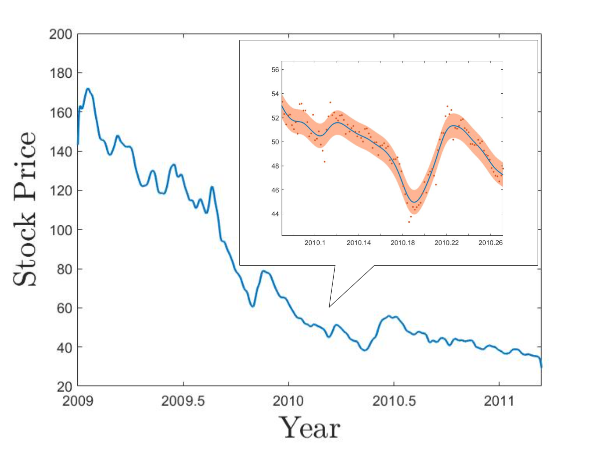
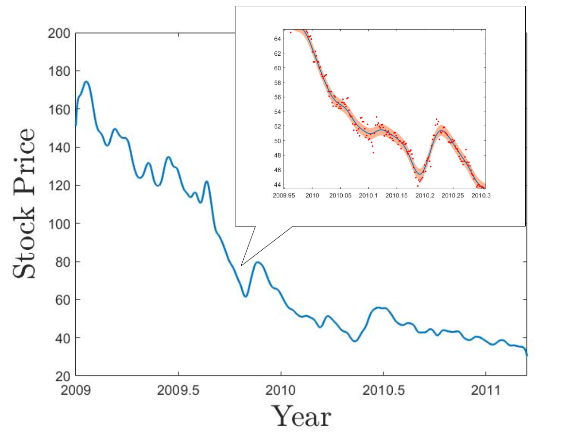
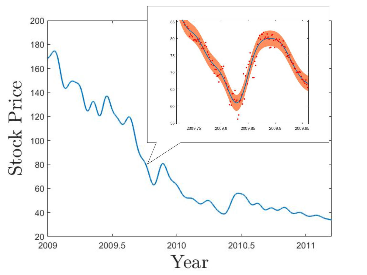
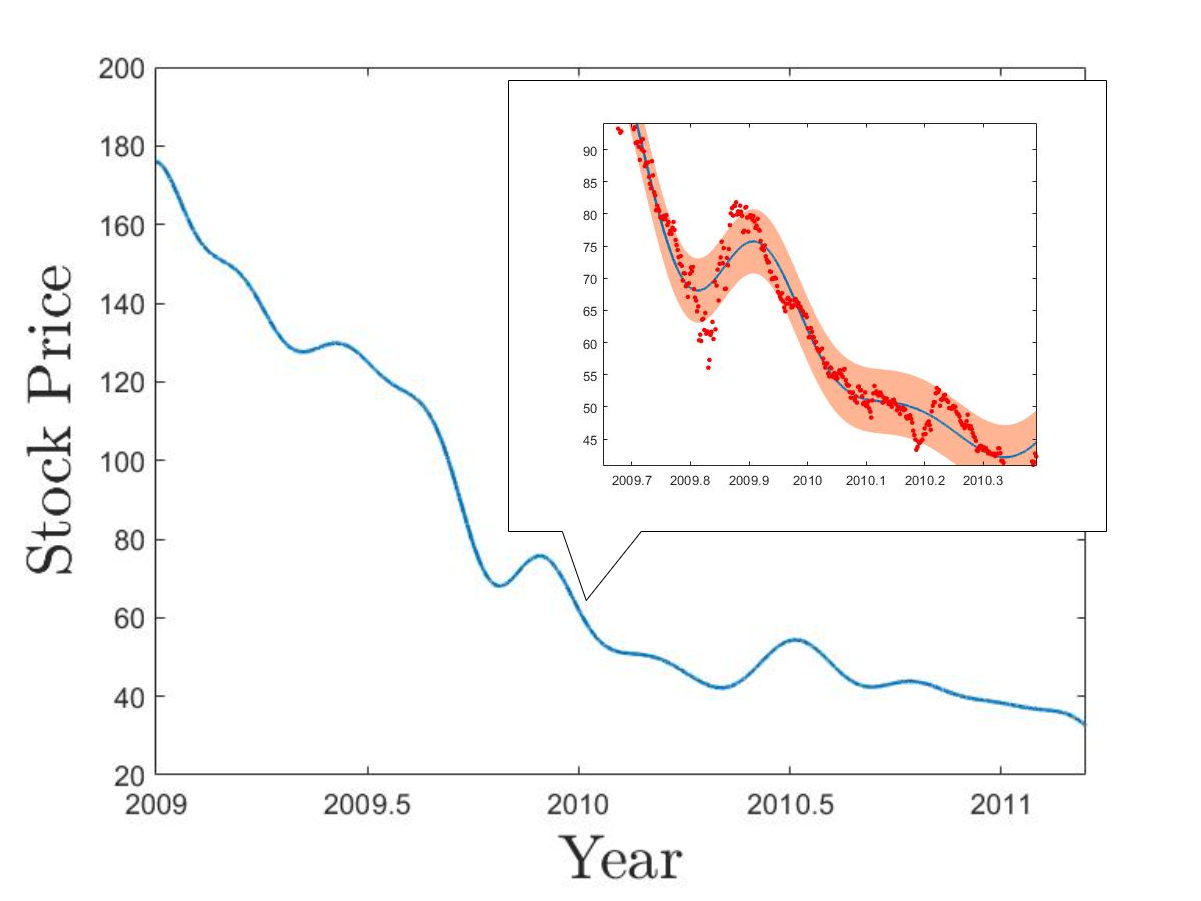
Similar to the previous experiment, Table 2 shows that the KP methods are more efficient than inducing points and RFF in both training and prediction. The predictive curve given by each algorithm is shown in Figure 7. We can see that both KP methods successfully capture the local changes of the overall trend while inducing points and RFF fail to do so. This is because neither inducing points nor RFF have enough number of feature functions to reconstruct curves with highly local fluctuations, and therefore, their predictive curves are too smooth so that a larger number of data points are distributed outside of their standard deviation areas.
5 Possible Extensions
Although the primary focus of this article is on exact algorithms, we would like to mention the potential of combining the proposed method with existing approximate algorithms. In this section, we will briefly discuss how to use the conjugate gradient method in the presence of the KP factorization (12) to accommodate a broader class of multi-dimensional Gaussian process regression problems.
5.1 Multi-dimensional GP Regression with Noisy Data
Suppose the input points lie in a full grid and the observed data is noisy: , where . Following arguments similar to what we have done in Sections 3.2 and 3.3, we can show that the following matrix operations are essential in computing the posterior and MLE:
| (31) | |||
| (32) |
for some . The direct Kronecker product approach fails to work in this scenario because the additive noise breaks the tensor product structure. Nonetheless, conjugate gradient methods such as those implemented in GPyTorch (Gardner et al., 2018) or MATLAB (Barrett et al., 1994) can be employed to solve (31) and (32) efficiently. This is because the conjugate gradient methods require nothing more than the multiplication between the covariance matrix and a vector. In our case, both and are banded matrices so and , which are Kronecker products of banded matrices, have only non-zero entries. Therefore, the cost of matrix-multiplications by the matres and both scale linearly with respect to the number of points in the grid. If input points lie in a sparse grid, the posterior and MLE conditional on noisy data can also be computed efficiently because they can be decomposed as linear combinations of posteriors and MLEs on full grids as shown in section 3.3.
5.2 Additive Covariance Functions
Suppose the GP is equipped with the following additive covariance function:
| (33) |
where is any subset of the power set of and is any one-dimensional Matérn correlation with half-integer smoothness. When input points lie in a full grid , the posterior and MLE can also be efficiently computed using conjugate gradient methods. In this case, the covariance matrix can be written as the following form:
| (34) |
The matrix-multiplication can be computed in linear time in the size of for any vector . Firstly, we use KLS techniques introduced in Section 3.3 to compute , which has linear time complexity in the size of . Then, we can compute , which has the same time complexity. Similar to Section 5.1, efficient algorithms also exist when input points lie in a sparse grid.
6 Conclusions and Discussion
In this work, we propose a rapid and exact algorithm for one-dimensional Gaussian process regression under Matérn correlations with half-integer smoothness. The proposed method can be applied to some multi-dimensional problems by using tensor product techniques, including grid and sparse grid designs, and their generalizations (Plumlee et al., 2021). With a simple modification, the proposed algorithm can also accommodate noisy data. If the design is not grid-based, the proposed algorithm is not applicable. We may apply the idea of Ding et al. (2020) to develop approximated algorithms, which work for not only regression problems, but also for other type of supervised learning tasks.
Another direction for future work is to establish the relationship between KP and the state-space approaches. The latter methods leverage the Gauss-Markov process representation of certain GPs, including Matérn-type GPs with half-integer smoothness, and employ the Kalman filtering and related methodologies to handle GP regression, which results in a learning algorithm with time and space complexity both in (Hartikainen and Särkkä, 2010; Saatçi, 2012; Sarkka et al., 2013; Loper et al., 2021). Whether the key mathematical theories of KP and state-space approaches are essentially equivalent is unknown and requires further investigation. Although having the same time and space complexity as KP, the Kalman filtering method is formulated in a sequential data processing form, which significantly differs from the usual supervised learning framework and makes it more difficult to comprehend. The proposed method, in contrast, is presented by a simple matrix factorization (12), which is easy to implement and incorporated in more complicated models.
Appendix
A Paley-Wiener Theorems
We will need two Paley-Wiener theorems in our proofs, given by Lemmas 15 and 16. For detailed discussion, we refer to Chapter 4 of Stein and Shakarchi (2003). Denote the support of function as .
Definition 14 (Stein and Shakarchi (2003), page 112)
We say that a function is of moderate decrease if there exists so that for some , for all .
Lemma 15 (Theorem 3.3 in Chapter 4 of Stein and Shakarchi (2003))
Suppose is continuous and of moderate decrease on , is the Fourier transform of . Then, has an extension to the complex plane that is entire with333Stein and Shakarchi (2003) uses an equivalent but different definition of the inverse Fourier transform as , so that this inequality becomes . for some , if and only if .
Lemma 16 (Theorem 3.5 in Chapter 4 of Stein and Shakarchi (2003))
Suppose is continuous and of moderate decrease on , is the Fourier transform of . Then if and only if can be extended to a continuous and bounded function in the closed upper half-plane with holomorphic in the interior.
B Technical Proofs
B.1 Algebraic Properties
The following Lemma 17 will be useful in proving the main theorems. We use to denote the degree of polynomial . For notational convenience, we define the degree of the zero polynomial as . We say a zero of function if .
Lemma 17
Let and be polynomials with . If and , then the function has at most real-valued zeros.
Proof
Without loss of generality, we assume that is non-zero. Suppose has at least real-valued zeros. Equivalently, the function
has at least real-valued zeros. The mean value theorem implies for some lying between two consecutive real-valued zeros of . Therefore, has at least real-valued zeros. Repeating this procedure times, we can conclude that has at least real-valued zeros. Note that possesses the form
where is a non-zero polynomial with degree . Because , has at least real-valued zeros, which contradicts the fundamental theorem of algebra.
Lemma 18 can directly lead to Theorems 2 and 9. We call the vector of zero the trivial solution to a homogeneous system of linear equations.
Lemma 18
The following homogeneous systems have only the trivial solutions.
-
1.
For , the system about :
with , and distinct real numbers .
-
2.
For , the system about :
(35) with , , and distinct real numbers .
Proof For both parts, it suffices to prove that the coefficient matrices are of full row ranks, which is equivalent to that they are of full column ranks. This inspires us to consider the transpose of the coefficient matrices.
Here we only provide the proof for Part 2. The proof for Part 1 follows from similar lines. For Part 2, the linear system corresponding to the transposed coefficient matrix is
| (36) |
with the vector of unknowns . Suppose (35) has a non-trivial solution. Then (36) also has a nontrivial solution, denoted as . Write and . Therefore, (36) implies that each is a zero of the function . Hence has at least distinct zeros. Note that . Because is non-trivial, we have . Thus Lemma 17 yields that has no more than distinct zeros, a contradiction.
Proof [Proof of Theorem 2]
This theorem follows directly from Part 2 of Lemma 18, because each submatrix of the coefficient matrix corresponds a linear system of the form in Part 2 of Lemma 18.
Proof [Proof of Theorem 9]
This theorem follows directly from Lemma 18, because each submatrix of the coefficient matrix corresponds a linear system of the form in of Lemma 18.
B.2 Results for the Supports
We first prove the following useful lemma.
Lemma 19
Let be a Matérn correlation with a half-integer smoothness. Suppose and for some . Let for . Denote , and . If there exists such that for , , then
Proof It is known that when with , the Matérn correlation can be expressed as (Santner et al., 2003)
| (37) |
where and is a polynomial of degree .
Therefore, for any ,
where and are polynomials. Thus is an analytic function on . Then for implies for , which is possible only if , because otherwise can only have at most distinct zeros on according to Lemma 17. Hence, whenever , and whenever .
The following lemma formalizes the rationale behind (8).
Lemma 20
Let be a connected open subset of containing a point . Let be a holomorphic function on , and a positive integer. Then can be extended as a holomorphic function on if and only if for ,
Proof First assume being holomorphic. Then must be zero, because otherwise . If vanishes identically in , the desired result is trivial. If does not vanish identically in , according to Theorem 1.1 in Chapter 3 of Stein and Shakarchi (2003), there exists a neighborhood of , and a unique positive integer such that for with being a non-vanishing holomorphic function on . Clearly it must hold that , because otherwise we have again. Then it is easily checked that for .
For the converse, in a small disc centered at the function has a power series expansion , where for each . Thus . Consequently, and thus is holomophic on .
Proof [Proof of Theorem 8] As before, let . Suppose that has a compact support. The analytic continuation of its inverse Fourier transform is
for . Then Lemma 20 entails for , which leads to the linear system
with and . But this system has only the trivial solution in view of Lemma 18.
Proof [Proof of Theorem 5]Without loss of generality, we can assume that and for some positive real number , because otherwise we can apply a shift translation to convert the original problem to this form in view of Theorem 3.
We first employ Lemma 15 to show that . Lemma 20 implies that is entire. By its continuity, is bounded in the region . For , we have
where the last inequality follows from the fact that Clearly, is of moderate decrease. According to Lemma 15, we obtain that .
It remains to prove that . Suppose . Then we can find , such that for . Therefore, Lemma 19 implies that can be expressed as
for some , such that . Because either or must not be identically vanishing, such a function, according to Definition 1, is a KP with degree less than . But this contradicts Theorem 8.
Proof [Proof of Theorem 7] For Part 1, when the smoothness parameter of a Matérn kernel is not a half integer, then direct calculations shows
| (38) | |||||
The goal is to prove that (38) cannot be extended to an entire function unless for each . There is no continuous complex logarithm function defined on all . Here we consider the principal branch of the complex logarithm where is the principal value of the argument of ranging in . For , we have . It is known that is holomorphic on the set . Therefore, the function in (38) can be analytically continued to the region
Because analytical continuation is unique, the analytical continuation of (38) should coincide with
on . Because is not an integer, is discontinuous when moves across . Suppose there exists a KP. Then must an entire function in view of lemma 15. To make continuous on , we must have on , but this readily implies on as is also an entire function. Therefore . By the uniqueness of the Fourier transform, the underlying KP vanishes identically in , which leads to a contradiction.
For part 2, a Gaussian correlation function is an analytic function on , and so does . Therefore, cannot have a compact support unless .
Proof [Proof of Theorem 11] Without loss of generality, we can assume that because otherwise we can apply shift translation to make this happen in view of Theorem 10.
Clearly, is of moderate decrease in view of the expression (37). Direct calculation shows
Equation (10) implies for . Thus for , which, together with Lemma 20, yields that is holomorphic in a neighborhood of . So is continuous on the upper half-plane and is holomorphic in its interior. To employ Lemma 16, it remains to proof that is bounded in . For , is clearly bounded as it is a continuous function. For and , we have
Write , then
which is bounded as . Therefore, according to Lemma 16, .
Next, we prove that . First, it can be shown that , because otherwise is a solution to the linear system with , if , or with and , if . Then Lemma 17 suggests that for all , which is a contradiction. Now, suppose . Then there exists , such that for all . Without loss of generality, assume . We now apply a shift transformation. Recall that . Theorem 10 implies that Thus,
It is easily seen that is unbounded if for sufficiently large . Specifically,
where the first term diverges and the second term converges to zero as , because and .
The remainder is to prove that . Suppose . Then there exist , such that whenever . Without loss of generality, we assume that . Then we can write
Then Lemma 19 implies that can be decomposed into
for some , such that and . Because , we have . Therefore, is a non-zero function and has a compact support, which contradicts Theorem 8.
B.3 Linear Independence
Proof [Proof of Theorem 13] We have learned from Theorems 5 and 11, and the analogous counterpart of Theorem 11 for the left-sided KPs that:
-
1.
The left-sided KPs have supports , , , , respectively.
-
2.
The KPs have supports , , , , respectively.
-
3.
The right-sided KPs have supports , , , respectively.
Therefore, for , any function of the form satisfies . Note that , which proves that . Hence, by induction, we can prove that are linearly independent.
Similarly, we can prove that the right-sided KPs are linearly independent.
Now suppose for . We rearrange this identity as
| (39) |
i.e., the left-hand side of (39) is a linear combination of the left-sided KPs and the KPs, and the right-hand side of (39) is a linear combination of the right-sided KPs.
Note that and . Then identify (39) implies .
By definition, is a linear combination of functions . Hence, by Theorem 8, has a compact support only if , which, together with the fact that are linearly independent, yields that . Then by (39), we similarly have because are proved to be linearly independent. In summary, we prove that are linearly independent.
References
- Atkinson (2008) Kendall E Atkinson. An Introduction to Numerical Analysis. John Wiley & Sons, 2008.
- Banerjee et al. (2014) Sudipto Banerjee, Bradley P Carlin, and Alan E Gelfand. Hierarchical Modeling and Analysis for Spatial Data. CRC press, 2014.
- Barrett et al. (1994) Richard Barrett, Michael Berry, Tony F Chan, James Demmel, June Donato, Jack Dongarra, Victor Eijkhout, Roldan Pozo, Charles Romine, and Henk Van der Vorst. Templates for the solution of linear systems: building blocks for iterative methods. SIAM, 1994.
- Bazi and Melgani (2009) Yakoub Bazi and Farid Melgani. Gaussian process approach to remote sensing image classification. IEEE transactions on geoscience and remote sensing, 48(1):186–197, 2009.
- Bui et al. (2017) Thang D Bui, Josiah Yan, and Richard E Turner. A unifying framework for gaussian process pseudo-point approximations using power expectation propagation. The Journal of Machine Learning Research, 18(1):3649–3720, 2017.
- Burt et al. (2019) David Burt, Carl Edward Rasmussen, and Mark Van Der Wilk. Rates of convergence for sparse variational gaussian process regression. In International Conference on Machine Learning, pages 862–871. PMLR, 2019.
- Chen and Stein (2021) Jie Chen and Michael Stein. Linear-cost covariance functions for gaussian random fields. Journal of the American Statistical Association, 2021. doi: 10.1080/01621459.2021.1919122.
- Cressie (2015) Noel Cressie. Statistics for spatial data. John Wiley & Sons, 2015.
- Davis (2006) Timothy A Davis. Direct Methods for Sparse Linear Systems. SIAM, 2006.
- Deisenroth et al. (2013) Marc Peter Deisenroth, Dieter Fox, and Carl Edward Rasmussen. Gaussian processes for data-efficient learning in robotics and control. IEEE transactions on pattern analysis and machine intelligence, 37(2):408–423, 2013.
- Ding et al. (2020) Liang Ding, Rui Tuo, and Shahin Shahrampour. Generalization guarantees for sparse kernel approximation with entropic optimal features. In Proceedings of the 37th International Conference on Machine Learning, pages 2545–2555, 2020.
- Fausett and Fulton (1994) Donald W Fausett and Charles T Fulton. Large least squares problems involving kronecker products. SIAM Journal on Matrix Analysis and Applications, 15(1):219–227, 1994.
- Gardner et al. (2018) Jacob R Gardner, Geoff Pleiss, David Bindel, Kilian Q Weinberger, and Andrew Gordon Wilson. Gpytorch: Blackbox matrix-matrix gaussian process inference with gpu acceleration. arXiv preprint arXiv:1809.11165, 2018.
- Gerstner and Griebel (1998) Thomas Gerstner and Michael Griebel. Numerical integration using sparse grids. Numerical Algorithms, 18(3):209–232, 1998.
- Graham (2018) Alexander Graham. Kronecker Products and Matrix Calculus with Applications. Courier Dover Publications, 2018.
- Gramacy (2020) Robert B Gramacy. Surrogates: Gaussian process modeling, design, and optimization for the applied sciences. Chapman and Hall/CRC, 2020.
- Gramacy and Apley (2015) Robert B Gramacy and Daniel W Apley. Local gaussian process approximation for large computer experiments. Journal of Computational and Graphical Statistics, 24(2):561–578, 2015.
- Hartikainen and Särkkä (2010) Jouni Hartikainen and Simo Särkkä. Kalman filtering and smoothing solutions to temporal gaussian process regression models. In 2010 IEEE international workshop on machine learning for signal processing, pages 379–384. IEEE, 2010.
- Hennig et al. (2015) Philipp Hennig, Michael A Osborne, and Mark Girolami. Probabilistic numerics and uncertainty in computations. Proceedings of the Royal Society A: Mathematical, Physical and Engineering Sciences, 471(2179):20150142, 2015.
- Jones et al. (1998) Donald R Jones, Matthias Schonlau, and William J Welch. Efficient global optimization of expensive black-box functions. J. Glob. Optim., 13(4):455–492, 1998.
- Kamgnia and Nguenang (2014) Emmanuel Kamgnia and Louis Bernard Nguenang. Some efficient methods for computing the determinant of large sparse matrices. Revue Africaine de la Recherche en Informatique et Mathématiques Appliquées, 17:73–92, 2014.
- Katzfuss (2017) Matthias Katzfuss. A multi-resolution approximation for massive spatial datasets. Journal of the American Statistical Association, 112(517):201–214, Jan 2017.
- Keeling and Whorf (2005) Charles D Keeling and TP Whorf. Atmospheric carbon dioxide record from mauna loa. Carbon Dioxide Research Group, Scripps Institution of Oceanography, University of California La Jolla, California, pages 92093–0444, 2005.
- Loper et al. (2021) Jackson Loper, David Blei, John P Cunningham, and Liam Paninski. A general linear-time inference method for Gaussian processes on one dimension. Journal of Machine Learning Research, 22(234):1–36, 2021.
- Molga and Smutnicki (2005) Marcin Molga and Czesław Smutnicki. Test functions for optimization needs. Test functions for optimization needs, 101:48, 2005.
- Plumlee et al. (2021) M Plumlee, CB Erickson, BE Ankenman, and E Lawrence. Composite grid designs for adaptive computer experiments with fast inference. Biometrika, 108(3):749–755, 2021.
- Plumlee (2014) Matthew Plumlee. Fast prediction of deterministic functions using sparse grid experimental designs. Journal of the American Statistical Association, 109(508):1581–1591, 2014.
- Rahimi and Recht (2007) Ali Rahimi and Benjamin Recht. Random features for large-scale kernel machines. In Advances in Neural Information Processing Systems 20, pages 1177–1184, 2007.
- Rasmussen (2006) Carl Edward Rasmussen. Gaussian Processes for Machine Learning. MIT Press, 2006.
- Rasmussen and Nickisch (2010) Carl Edward Rasmussen and Hannes Nickisch. Gaussian processes for machine learning (gpml) toolbox. Journal of Machine Learning Research, 11(100):3011–3015, 2010.
- Saatçi (2012) Yunus Saatçi. Scalable inference for structured Gaussian process models. PhD thesis, Citeseer, 2012.
- Sacks et al. (1989) Jerome Sacks, William J Welch, Toby J Mitchell, and Henry P Wynn. Design and analysis of computer experiments. Statistical science, 4(4):409–423, 1989.
- Santner et al. (2003) Thomas J Santner, Brian J Williams, William I Notz, and Brain J Williams. The Design and Analysis of Computer Experiments, volume 1. Springer, 2003.
- Sarkka et al. (2013) Simo Sarkka, Arno Solin, and Jouni Hartikainen. Spatiotemporal learning via infinite-dimensional bayesian filtering and smoothing: A look at gaussian process regression through kalman filtering. IEEE Signal Processing Magazine, 30(4):51–61, 2013.
- Smola and Schölkopf (2000) Alex J Smola and Bernhard Schölkopf. Sparse greedy matrix approximation for machine learning. 2000.
- Srinivas et al. (2009) Niranjan Srinivas, Andreas Krause, Sham M Kakade, and Matthias Seeger. Gaussian process optimization in the bandit setting: No regret and experimental design. arXiv preprint arXiv:0912.3995, 2009.
- Sriperumbudur and Szabo (2015) Bharath Sriperumbudur and Zoltan Szabo. Optimal rates for random fourier features. Advances in Neural Information Processing Systems, 28:1144–1152, 2015.
- Stein and Shakarchi (2003) Elias M Stein and Rami Shakarchi. Complex Analysis. Princeton University Press, 2003.
- Stein (1999) Michael L Stein. Interpolation of Spatial Data: some theory for kriging. Springer Science & Business Media, 1999.
- Titsias (2009) Michalis Titsias. Variational learning of inducing variables in sparse gaussian processes. In Artificial intelligence and statistics, pages 567–574. PMLR, 2009.
- Tuo and Wang (2020) Rui Tuo and Wenjia Wang. Kriging prediction with isotropic matern correlations: robustness and experimental designs. Journal of Machine Learning Research, 21(187):1–38, 2020.
- Tuo and Wu (2016) Rui Tuo and C. F. Jeff Wu. A theoretical framework for calibration in computer models: parametrization, estimation and convergence properties. SIAM/ASA Journal on Uncertainty Quantification, 4(1):767–795, 2016.
- Williams and Seeger (2001) Christopher Williams and Matthias Seeger. Using the Nyström method to speed up kernel machines. In Proceedings of the 14th Annual Conference on Neural Information Processing Systems, pages 682–688, 2001.
- Wilson and Nickisch (2015) Andrew Wilson and Hannes Nickisch. Kernel interpolation for scalable structured Gaussian processes (kiss-gp). In International Conference on Machine Learning, pages 1775–1784, 2015.
- Wilson (2014) Andrew Gordon Wilson. Covariance kernels for fast automatic pattern discovery and extrapolation with Gaussian processes. PhD thesis, Citeseer, 2014.
- Wood and Chan (1994) Andrew TA Wood and Grace Chan. Simulation of stationary Gaussian processes in . Journal of Computational and Graphical Statistics, 3(4):409–432, 1994.
- Zhang et al. (2005) Yunong Zhang, William E Leithead, and Douglas J Leith. Time-series gaussian process regression based on toeplitz computation of operations and -level storage. In Proceedings of the 44th IEEE Conference on Decision and Control, pages 3711–3716. IEEE, 2005.