Key frames assisted hybrid encoding for photorealistic compressive video sensing
Abstract
Snapshot compressive imaging (SCI) encodes high-speed scene video into a snapshot measurement and then computationally makes reconstructions, allowing for efficient high-dimensional data acquisition. Numerous algorithms, ranging from regularization-based optimization and deep learning, are being investigated to improve reconstruction quality, but they are still limited by the ill-posed and information-deficient nature of the standard SCI paradigm. To overcome these drawbacks, we propose a new key frames assisted hybrid encoding paradigm for compressive video sensing, termed KH-CVS, that alternatively captures short-exposure key frames without coding and long-exposure encoded compressive frames to jointly reconstruct photorealistic video. With the use of optical flow and spatial warping, a deep convolutional neural network framework is constructed to integrate the benefits of these two types of frames. Extensive experiments on both simulations and real data from the prototype we developed verify the superiority of the proposed method.
1 Introduction
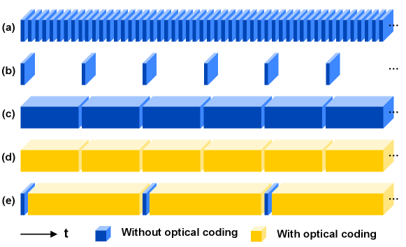
Sensing of high-speed scene is widely desirable in applications of robotics, autonomous driving, scientific research, etc. As illustrated in Fig. 1(a), conventional high-speed cameras directly capture such scenes at a high frame rate, while imposing challenges on hardware manufacturing, data readout, transferring, processing, and storage, resulting in massive data sizes and high costs of use. With a low frame rate, off-the-shelf ordinary cameras suffer from loss of interframe information with short exposure [Fig. 1(b)] or motion blur with long exposure [Fig. 1(c)] when capture fast events.
Different from the conventional imaging systems with brute-force sampling strategies, computational imaging [1] jointly develops the opto-electronic hardware and the back-end algorithms to realize novel imaging properties. As an important branch of computational imaging, inspired by compressive sensing (CS) theory [2], video snapshot compressive imaging (SCI) [3] encodes multiple frames into a single snapshot and then computationally makes reconstruction to enable high-speed scene recording with a low-frame-rate sensor [Fig. 1(d)]. To achieve optimal video quality, innovations in both hardware encoder and software decoder techniques have been made in recent years.
Standard video SCI systems [3] utilize a series of temporally varying masks to modulate dynamic scene frames at different times, then operate temporal integration through the exposure of the imaging sensor to form a snapshot measurement, namely, a compressive frame. Early video SCI systems [4, 5] mechanically translate a static lithography mask to generate temporally varying coding, which faces the challenges of inaccuracy or instability. Currently, mainstream SCI systems use spatial light modulators (SLM) for encoding, such as digital micromirror device (DMD) [6, 7, 8] and liquid crystal on silicon (LCoS) [9, 10], which enable accurate and flexible pixel-wise exposure control. Recently, extensions to the basic SCI scheme have been developed to enhance the encoding processing. To extend the field-of-view (FoV), the frames of two FoVs are compressed into a snapshot by polarization multiplexing [6, 7]. To improve the spatial resolution of the coding video, the SLM and the static mask can be cascaded to provide finer encoding patterns [9]. Taking advances in deep optics [11], diffractive optical elements (DOEs) have been inserted into the optical path to form an optimized point spread function (PSF) and thus realize spatial superresolution in SCI [10].
In parallel with hardware systems, research in the field of SCI has also dived deep into the design of reconstruction algorithms. Conventional algorithms employ regularization-based optimization to solve the ill-posed inversion problem. Numerous regularization items, such as total variant (TV) [12], non-local low rank [13], Gaussian mixture model (GMM) [14, 15], and deep denoisers in plug-and-play (PnP) approaches [16, 17] serve as priors in optimization frameworks like the alternating direction method of multipliers (ADMM) [18] or generalized alternating projection (GAP) [19]. These methods are training-free and flexible to different coding but highly time-consuming with hundreds of iterations. Recently, deep neural networks are employed to learning an end-to-end (E2E) mapping from the encoded measurement to the reconstruction video and various network architectures have been proposed. E2E-CNN [8] uses a fully convolutional network with skip-connections, which significantly reduces the reconstruction time. BIRNAT [20] reconstructs the video frames with bidirectional recurrent neural networks (RNN). RevSCI [21] based on multi-group reversible 3D convolutional neural networks has led to state-of-the-art reconstruction results. Taking advantage of advances in the deep unfolding framework, ADMM-net [22] unrolls the ADMM iteration loop into an E2E network with a few stages with fast speed and interpretability.
Although sophisticated hardware systems and novel algorithms have been developed to make remarkable progress in SCI, it is still challenging to further improve the visual quality of the reconstructed video. Regardless of implementation differences, they follow the same basic SCI paradigm of extracting multiple frames from a fully blurred compressive frame. The process of video reconstruction is an under-determined inverse problem with inherently high ill-posedness, where a theoretical upper bound of performance is imposed for current paradigm [23]. To some extent, the lack of information can be compensated by the priors/regulators or the implicit information contained in trained deep models, making it possible to recover the crude scene appearance. Nonetheless, the recovery of fine details or complicated texture is still arduous. Our insight is that, although lacking dynamic information, short-exposure images can provide a wealth of spatial details, which act conceptually akin to key frames in digital video compression [24]. Taking consideration of the temporal consistency of natural scenes, we can alternately sample compressive frames and short-exposure key frames in a hybrid manner and then fuse the two to take both merits for photorealistic reconstruction.
In the field of computational imaging and machine vision, the concept of data fusion is widely established to exploit the complementary properties of multiple sensing modalities. For example, depth data such as steroid camera images, LiDAR point clouds, and radar signals can be fused to enhance the 3D perception [25]. In hyperspectral imaging, by fusion of low-resolution hyperspectral images (LR-HSI) with high-resolution multispectral images (HR-MSI) [26], or RGB images with the coded aperture snapshot spectral imaging (CASSI) system [27, 28], the spectral sensing capability can be significantly improved. The event flows provided by a dynamic vision sensors (DVS) can help to ease the motion blur in the images captured by ordinary cameras [29]. Cameras with different spatial-temporal properties can also cooperate to synthesize high-resolution videos [30, 31, 32]. Images captured with different exposure setups are fusion to enhanced the performance of low-light imaging and dynamic range [33]. Under the topic of compressive video sensing, SCI systems can cooperate with long-exposure blurred images captured by standard cameras without coding, to serve as side information (SI) for video reconstruction [34] or jointly reconstruct high-speed stereo video [35], but extracting fine details from two blur measurements remains challenging. Furthermore, geometric calibration of cameras is necessary in such scheme, and the data size and expenses are doubled as one more camera is added. Fortunately, the SLMs utilized in currently mainstream SCI systems provide flexible pixel-wise shutter control, enabling compressive frames and short-exposure key frames to be acquired without the need for additional hardware.
In this paper, we propose a new hybrid sampling paradigm for compressive video sensing, dubbed KH-CVS. We alternatively samples short-exposure key frames without coding and long-exposure compressive encoded frames to jointly reconstruct high-speed video. To fuse the hybrid-sampled data, a deep-learning-based reconstruction model is developed. Especially, the optical flow information is leveraged to deal with spatial movements in the dynamic scene. We built a hardware prototype to enable the hybrid sampling scheme. Validated by both numerical evaluation and hardware experiments, the proposed KH-CVS system has been demonstrated superior to conventional snapshot-based methods for photorealistic compressive video sensing.
2 Methods
2.1 Hardware Experiments
The optical setup of the KH-CVS prototype built by us is shown in Fig. 2(a). A camera lens forms an image at the focal plane, where a DMD (ViALUX V-9001, 2560 × 1600 resolution, 7.6 um pitch size) is located. After modulated by the DMD, the image is then transferred to an image sensor (FLIR GS3-U3-123S6M-C, 4096 × 3000 resolution, 3.45 um pixel size) by a projection lens with a magnification rate of for a pixel-to-pixel mapping. Through the exposure of the image sensor, the measurements can be yielded and readout. The micromirrors on the DMD can be individually rotated to reflect the light to different directions, leading to an on-off state control. A total internal reflection (TIR) prism [36] is used to steerer the light from the camera lens, making it incident onto the DMD surface at to meet the angle condition of the DMD. Since it is difficult to directly measure the mismatch between the DMD and the image sensor, a Moire-fringe-based approach proposed by [37] is utilized to align these two elements. In the practice, to fit the spatial resolution of 256 256 in the deep model, we perform 6 6 binning, i.e., capture an region of interest (ROI) of 1536 1536 and then manually downsample by a factor of 6. In order to exclude the ambient light and increase the stability of the system, we package the optical system to build a prototype, of which a photograph is shown in Fig. 2(b).
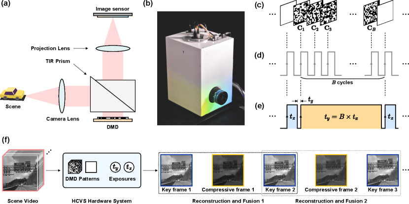
Since KH-CVS needs to alternately capture short-exposure key frames without coding and long-exposure compressive frames with coding, it is required to design a timing scheme that differs from that used in standard SCI systems. As illustrated in Fig. 2(c), among the preloaded patterns on the DMD, there are coding patterns ( to ) and an additional fully open pattern that all micromirrors are "on" (the DMD works as an ordinary reflective mirror with this pattern). We generate and synchronize the DMD and image sensor control signals through an arbitrary waveform generator (AWG, UNI-T UTG2000B). For the DMD, its trigger signal is a periodic rectangular wave with its period identical to the equivalent exposure time , and the DMD refreshes the pattern at each rising edge [Fig. 2(d)]. For the image sensor, the trigger signal is an alternating short and long rectangular wave [Fig. 2(e)]. The short pulse width is and corresponds to a key frame. The duration of the long rectangular wave is , and coding patterns will be consecutively refreshed on the DMD within this exposure, producing a compressive frame. In this manner, a sequence of alternate key frames and compressive frames is captured. A small temporal interval is set between two exposures of the image sensor for data readout and sensor cleaning.
The conceptual pipeline of KH-CVS is depicted in Fig. 2(f). With the aforementioned setup of DMD patterns and trigger signals, the scene video with high temporal dimension is encoded and captured as a sequence of key frames and compressive frames. Similar to standard SCI, frames can be recovered from each compressive, which is then fused with its neighboring two key frames, as indicated by the black dotted box. For compressive frame 1, key frame 1 and 2 are referred to as left and right key frame. Key frame 2 is also reused as the left key frame for compressive frame 2 in the gray dotted box. Thus, averaged 2 frames are capable of producing frames ( reconstructed frames and 1 key frames itself) in KH-CVS, which leads to a compressive ratio as from a systematic viewpoint.
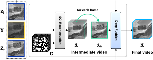
As illustrated in Fig. 3, in the algorithm, an intermediate reconstructed video is first made with a standard SCI method, and then each frame of it is fused with the two key frames by a deep fusion module (Fig. 4). The detailed methods are introduced as below.
2.2 Standard Video SCI
In the mathematical model of standard video SCI, a high-speed dynamic scene video containing frames with spatial resolution , is modulated by a coding cube , which contains encoding masks . In general, pre-generated pseudo-random patterns are established for encoding in SCI systems. During the long exposure time of the image sensor, the coded frames are temporally integrated to produce a coded compressive frame , which is
| (1) |
where represents the measurement noise and denotes the Hadamard product, which can be expressed in detail as
| (2) |
where and denote spatial positions and , , , are elements of , , , , respectively. By taking the prior-known encoding masks and the compressive frame as inputs, a reconstruction algorithm for standard SCI is applied to estimate the scene video , which contains reconstructed frames :
| (3) |
and the equivalent exposure time of each frame of the reconstruction video is , thus the equivalent frame rate is boosted by times. For standard SCI, is the output as the final results, but in KH-CVS, it acts as an intermediate reconstruction, which is then fused with the key frames to achieve enhanced visual quality.
2.3 Hybrid Sampling and Deep Fusion
In the proposed KH-CVS, the short-exposure key frames and the long-exposure encoded frames are alternatively sampled, as shown in Fig. 2(f). For each compressive frame , its two neighboring short-exposured key frames are
| (4) |
To match the equivalent exposure time , the exposure time of the key frames is set to . As illustrated in Fig. 3, each frame in is sequentially fused with and to produce the corresponding output frame by the fusion module shown in Fig. 4:
| (5) |
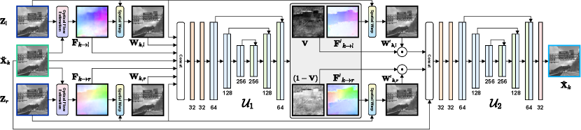
Although the key frames contain delicate visual details, there are movements between them and the intermediate frame, causing the features or contents of them to be spatially misaligned, posing a major difficulty for image fusion. To overcome this problem, we incorporate the optical flow [38] into the model, which is able to reveal the moving velocity and direction of each pixel between two frames. As a widely used technique, optical flow can be calculated with an off-the-shelf estimator, noted as . Then, the key frames can be spatially warped to align with the target intermediate frame for further fusion. To this end, the first step is to estimate the optical flow from the th intermediate frame to and ,
| (6) |
Then using a spatial warping function , which is an interpolation operation [38] based on the optical flow, the two key frames are warped to the target frame as
| (7) |
Due to the relatively low quality of intermediate frames, the optical flows and warped frames in this stage are relatively rough. Thus, a neural network is used to refine optical flows by estimating their residuals. Moreover, intuitively, if the target frame is temporally near to the left keyframe, the contribution of the warped left keyframe to the final fused frame should be weighted more, and vice versa. Thus, a visible map is introduced to weight the pixel values taken from two warped keyframes, which is inspired by [39]. We use one output channel of with an sigmoid function to yield a visible map between [0,1] to weight left keyframe and use for right keyframe.
| (8) |
Thus, the refined optical flows are calculated by
| (9) |
which are used to warp the key frames as
| (10) |
Finally, another network is used to make the final output frame by synthesizing the visible maps, warped key frames with optimal optical flows, and the intermediate frame:
| (11) |
Using the same method, all frames in are processed and combined to form the final video .
2.4 Model implementation and network training
The KH-CVS is a flexible framework that allows for a variety choices of submodules. For the demonstration in this work, E2E-CNN [8] is adopted as the basic SCI reconstruction model . For optical flow calculation, taking both efficiency and precision into account, a well-established PWC-Net [40] is used as optical flow estimator . To improve the accuracy of the optical flow, instead of directly calculate , we calculate , and combine the relatively small movements revealed by this set of optical flows to form . As illustrated in Fig. 4, the networks and are based on U-Net [41]. Inspired by [42, 32], the shallow layers in CNN are able to extract edges and textures as contextual information to help produce better results. Therefore, we use the first convolutional layer in a ResNet18 [43] to extract the feature maps of the frames and concatenate them together before feeding them into . In order to improve the ability of the network to handle spatial deformation, at the end of , a deformable convolutional layer [44] is applied to synthesize deep latent features to produce the final output.
The model is trained in a multi-stage manner. First, the SCI reconstruction model is trained following the configuration of the corresponding SCI model (which is E2E-CNN here). For the loss function, the L1 distance is adopted here, which is more favorable than L2 distance in image restoration tasks [45]. Thus, the loss function of this stage is
| (12) |
Then, the optical flow refinement model is trained. Given that is not ready at this stage, we can use the aforementioned visible map to form a linear combination of two warped keyframes to supervise the training of ,
| (13) |
where is a time factor that indicates the relative temporal distance to the left and right key frames. To supervise both synthesized frames and warped frames, the loss function for training is
| (14) |
Finally, is trained using the loss calculated with the final output as
| (15) |
The proposed architecture is implemented in PyTorch with two NVIDIA RTX 3090 GPUs. Adam optimizer [46] is used to train the model, with its parameters and set to 0.5 and 0.999. For training of the basic SCI model , the learning rate is set to for 100 epochs and then for another 100 epochs. Then the trained is fixed and is trained with the same setup of learning rate and epoch number, with and set to 200 and 100, respectively. Next, is connected to the model and trained 50 epochs with an initial learning rate of and then for another 50 epochs. Finally, the whole model is jointly trained for 50 epochs at a learning rate of . For model training, 5000 video clips are sampled from the ImageNet VID [47] training set and randomly cropped to 256 256, with horizontal flipping randomly for data augmentation. Each video clip has 16 continuous frames (thus ) with their two neighbored key frames to serve as network inputs.
3 Experiments
3.1 Simulation Experiments
| Metrics | Methods | Road-sign | Vehicle | Fox | Grass | Indoor | Lizard | Average |
|---|---|---|---|---|---|---|---|---|
| PSNR | GAP-TV | 22.94 | 24.75 | 23.52 | 24.27 | 28.22 | 24.31 | 24.67 |
| PnP-FFDNet | 22.07 | 24.10 | 22.58 | 24.27 | 30.69 | 23.92 | 24.61 | |
| PnP-TV-FastDVDNet | 26.42 | 28.36 | 26.44 | 28.09 | 34.98 | 26.17 | 28.41 | |
| BIRNAT | 29.32 | 28.77 | 26.73 | 28.81 | 37.50 | 29.78 | 30.15 | |
| RevSCI | 29.78 | 30.30 | 28.47 | 29.56 | 38.11 | 30.77 | 31.16 | |
| E2E-CNN-8 | 28.63 | 28.49 | 25.51 | 27.52 | 34.58 | 27.88 | 28.77 | |
| E2E-CNN-16 | 27.45 | 26.84 | 24.19 | 26.12 | 31.63 | 26.34 | 27.10 | |
| KH-CVS (proposed) | 31.62 | 29.79 | 29.84 | 32.14 | 37.27 | 32.58 | 32.21 | |
| SSIM | GAP-TV | 0.7885 | 0.7938 | 0.6193 | 0.6544 | 0.8842 | 0.6817 | 0.7370 |
| PnP-FFDNet | 0.7884 | 0.7975 | 0.5940 | 0.6634 | 0.9441 | 0.6730 | 0.7434 | |
| PnP-TV-FastDVDNet | 0.9090 | 0.8991 | 0.7988 | 0.8120 | 0.9691 | 0.7906 | 0.8631 | |
| BIRNAT | 0.9520 | 0.9127 | 0.8203 | 0.8410 | 0.9817 | 0.8992 | 0.9012 | |
| RevSCI | 0.9560 | 0.9356 | 0.8801 | 0.8644 | 0.9837 | 0.9213 | 0.9235 | |
| E2E-CNN-8 | 0.9459 | 0.9036 | 0.7383 | 0.7925 | 0.9709 | 0.8374 | 0.8648 | |
| E2E-CNN-16 | 0.9254 | 0.8537 | 0.6227 | 0.7241 | 0.9464 | 0.7607 | 0.8055 | |
| KH-CVS (proposed) | 0.9689 | 0.9279 | 0.9175 | 0.9416 | 0.9808 | 0.9460 | 0.9471 | |
| LPIPS | GAP-TV | 0.2934 | 0.2671 | 0.3507 | 0.3945 | 0.2314 | 0.3001 | 0.3062 |
| PnP-FFDNet | 0.2802 | 0.2651 | 0.4322 | 0.4005 | 0.0716 | 0.3387 | 0.2980 | |
| PnP-TV-FastDVDNet | 0.1028 | 0.1010 | 0.1551 | 0.1591 | 0.0391 | 0.1574 | 0.1191 | |
| BIRNAT | 0.0598 | 0.0806 | 0.1259 | 0.1556 | 0.0180 | 0.0745 | 0.0857 | |
| RevSCI | 0.0492 | 0.0567 | 0.1065 | 0.1328 | 0.0129 | 0.0547 | 0.0688 | |
| E2E-CNN-8 | 0.0752 | 0.1214 | 0.2412 | 0.2491 | 0.0404 | 0.1461 | 0.1456 | |
| E2E-CNN-16 | 0.1120 | 0.1942 | 0.3487 | 0.3517 | 0.0892 | 0.2068 | 0.2171 | |
| KH-CVS (proposed) | 0.0316 | 0.0465 | 0.0518 | 0.0446 | 0.0195 | 0.0380 | 0.0387 |
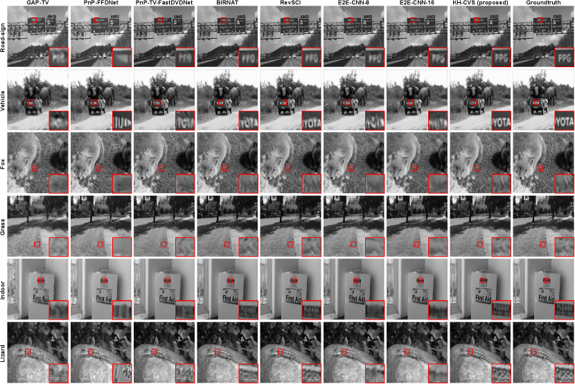
A series of simulation experiments are conducted to investigate the performance of the proposed KH-CVS on simulated datasets from ImageNet VID [47] test set and NFS [48], including Road-sign, Vehicle, Fox, Grass, Indoor and Lizard. Multiple existing algorithms are used for comparison, including GAP-TV [12], PnP-FFDNet [16], PnP-TV-FastDVDNet [9], BIRNAT [20] and RevSCI [21]. According to the analysis in Sec.2, the compressive ratio is , i.e., 11.67% for . In order to conduct a fair comparison, the systematic compressive ratio of the competitive counterpart algorithms should not be lower than KH-CVS, ensuring sufficient data amount for the counterparts. Therefore, for the counterparts, the same 16 frames are reconstructed from two snapshot (each encodes 8 frames in standard SCI paradigm), which corresponds to a compressive ratio of 12.5%. As the basic SCI model used in KH-CVS, the E2E-CNN [8] is also compared. E2E-CNN-8 and E2E-CNN-16 represent the models trained with and , respectively.
Fig. 5 shows the exemplary frames of the reconstructed videos, which validates that KH-CVS is capable of providing higher visual quality with more fine details. The baseline models GAP-TV results suffer from strong noise and the PnP-FFDNet produces unpleasant artifacts. Among the countpart methods, the state-of-the-art algorithm RevSCI shows the best performance, yet the details in the reconstruction are relatively blurry and distorted (like the characters in scene Road-sign and Vehicle). In the basic E2E-CNN-16 model of KH-CVS, Details are also blurred out, but rough outlines are reserved. By fusion of the information from the key frames, the details can be well compensated to obtain high-quality reconstructions.
To quantitatively evaluate reconstruction quality, multiple metrics are used, including widely-used peak signal to noise ratio (PSNR) [49], structural similarity index measure (SSIM) [49]. In addition to these classic metrics, the learned perceptual image patch similarity (LPIPS) [50] is also used to evaluate perceptual visual quality, which is calculated in the deep feature space as perceptual distance. Note that a lower LPIPS means the reconstructions are more similar to the ground-truths. Since the key frames are identical to their corresponding ground-truth frames in the simulation, metrics are calculated only on the reconstructed frames to prevent privilege of KH-CVS. Quantitative results are summarized in Tab. 1. It can be observed that the proposed KH-CVS achieves 1.05 dB improvement in PSNR and 0.0236 in SSIM on average, compared to the best results of counterparts, i.e., RevSCI. KH-CVS reduces the averaged LPIPS to about half of RevSCI, which reveals that the KH-CVS reconstruction frames are perceptually more closed to the ground-truth frames. It is also worth mentioning that, compared to its basic SCI model E2E-CNN-16, KH-CVS boosts PSNR by 5.11 dB and SSIM by 0.1416, and decreases LPIPS to about only 17.8% of itself, which shows that the information from the key frames can help significantly improve the performance of the basic SCI model.
3.2 Visualization of Intermediate Results in the Pipeline
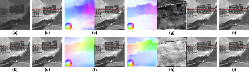
The inputs and intermediate results of the model are visualized in Fig. 6. Here the 12th frame is used as an example. To visualize the optical flow field, we color code the optical flow field following [38], that is, using the color hue to represent the direction of motion and the saturation to represent the magnitude. In the scene of Road-sign, as the vehicle moves forward, the road-sign are from far to near, so from the left key frame to , the road signs are expanded outward, and the preliminarily estimated optical flow is consistent with this observation. Through this optical flow, can be warped to as . Because is relatively rough, the warp results also have errors (such as the position of the characters and the edge of the image). After refinement, the optical flow is more accurate and can distinguish the area of the road-sign with a displacement and the area of the relatively static background. At this time, the warped result is also enhanced. The behavior of the right key frame is similar to that mentioned above. Since is temporally nearer to here, it is supposed to provide more information than , which is also consistent with that revealed by the visible map . It can be seen that, compared to the intermediate reconstructed frame , the final output frame has a significant improvement in the details of the scene, which is closer to the ground-truth .
3.3 Validation of the Robustness to the Frame Gap
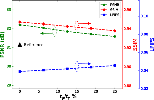
In the process of capturing, the image sensor needs time to readout the image data and clear the sensor to prepare for next image, thus the frame gap (noted as ) exists in real systems. This gap also occurs between two snapshot in the standard SCI. Since KH-CVS fuses multiple frames to make reconstruction with considering temporal consistency of the scene, its robustness to the gap between measured frames is needed to be evaluated. In this subsection, a series of experiments on simulated datasets are conducted to evaluate the robustness to the frame gap. In the ideal case, the frames to be compressed and the two key frames are continuously sampled from the video dataset. In order to simulate the actual frame gap, we skip some frames between the key frames and compressive frames during this test. For example, when , it means that there are 2 skipped frames between the left key frame and the first compressive frame , and also 2 frames between and , thus the normalized frame gap . In order to evaluate the effect of frame gap on reconstruction quality, we sweep the frame gap from 0 to 4 frames, corresponding to the changing from 0 to 25%, and the results are presented in Fig. 7. It can be seen from the results that with the increase of the , the quality of reconstruction decreases, but the trend is relatively slight. From the ideal situation to , the PSNR drops by 0.61 dB, the SSIM drops by 0.0092, and the LPIPS rises by 0.0066, while all metrics are still better than the best of the counterpart methods (marked by the black triangle). This shows that KH-CVS is robust to the frame gap. We experimentally found that setting as 300 is enough for preventing missing the next trigger pulse and allows a continuously sampling. For the demonstration in this paper, , is 33328 (see below) , resulting in less than 1%. Thus the reconstruction model is capable to deal with the frame gap in this system setup.
3.4 Hardware Experiments
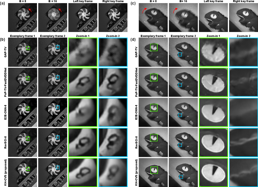
We used the KH-CVS prototype to record the actual scenes, and the experimental results are shown in Fig. 8. We compare KH-CVS () with standard SCI () in the same scene. The period of DMD trigger signal is set to 2083 , corresponding to an equivalent frame rate of about 480 frame per second (fps). In KH-CVS, the duration of short exposure is also 2083 and that of long exposure is set to 33328 . For standard SCI, the exposure time of compressive frames is set to 16664 , which is approximately half to that of KH-CVS, so that the equivalent frame rates in the reconstructed videos of the two systems are kept equal. Note that due to the difference of exposure setups, the brightness of captures are different. In the experiments, the short exposed keyframes are darker than the compressive frames. Before entering the algorithms, they are normalized to keep the same mean value to the intermediate reconstruction frames. This strategy is a common operation that can be also seen in burst high-dynamic-range imaging [51]. For reconstruction, GAP-TV, PnP-TV-FastDVDNet, E2E-CNN-8 and RevSCI are used for standard SCI, and the KH-CVS results are reconstructed using the model proposed in this paper (the basic SCI model in KH-CVS is E2E-CNN-16). Based on this setup, first, a rotating fan, with letters marked on several blades of the it, serves as the target scene. The measurements and key frames [Fig. 8 (a)], the reconstructions [Fig. 8 (b)] of standard SCI methods and KH-CVS are shown. In all standard SCI results, the rough outline of the fan blade can be recovered, but the details are relatively blurred and severely distorted by strong artifacts. In the KH-CVS results, the stroke of the character can be clearly recovered. In another scene, we capture a moving toy dinosaur [Fig. 8 (c)-(d)]. Since the object is moved manually and the compressive frames of and are captured one after another, the location of the objects and the motion trajectories are not strictly identical. In the results of standard SCI, the texture of the eye of the toy dinosaur is difficult to resolve with its shape distorted, and the teeth are also blurred. In the results of KH-CVS, the surface texture and edges can be clearly seen with the oval shape of the eye well maintained, and details of the teeth can also be recovered, which also reveals that KH-CVS works well for both bright and dark areas. The results show that the KH-CVS proposed in this paper can achieve better visual quality than standard SCI in real high-speed scenes.
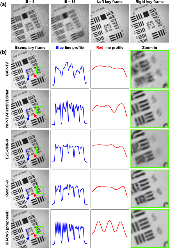
To further test the reconstruction quality of KH-CVS, we used a moving USAF 1951 resolution chart as a target. Note that the resolution chart here was printed by us, which is different from its original scale, but can still be used for relative resolution comparison. Measurements for standard SCI and KH-CVS and key frames are shown in Fig. 9(a). Exemplary reconstructed frames are shown in Fig. 9(b), along with line profiles and zoomed-in views. The blue line plots the horizontal part of group 2, elements 2 to 6, and the red line shows the profiles of group 2, element 1 (vertical parts). For the line profiles, the vertical axis is the grayscale pixel value (from 0 to 255), and the horizontal axis is the normalized spatial distance. The zoomed-in views show the details at group 1, element 5 and 6. In the standard SCI results obtained by the counterpart methods, the bars are affected by strong artifacts and distorted, and the digits are completely blurred. In KH-CVS, they can be clearly distinguished, with better contrast and almost no artifacts.
4 Discussion and Conclusions
In summary, KH-CVS offers a new paradigm for compressive video sensing, which brings in benefits to effectively improve the visual quality of reconstructed video. KH-CVS breaks through the standard SCI paradigm that makes reconstruction rely only on a single compressive frame, alternately captures long-exposure compressive frames and short-exposure key frames, and fuses their information to achieve photorealistic compressive video sensing. To this end, we designed a deep neural network architecture that includes basic SCI reconstruction, optical flow estimation, and fusion modules. Through simulation experiments, we verified that KH-CVS has advantages over multiple reconstruction methods [12, 16, 9, 20, 21, 8] of standard SCI with the same level of data amount. Based on our built prototype, we captured actual dynamic scenes at an equivalent frame rate of 480 fps, and the experimental results show that KH-CVS can achieve high visual quality video reconstruction with a wealth of fine details.
KH-CVS is a flexible framework. For the algorithm, we use E2E-CNN as the base model for basic SCI reconstruction, as demonstrated in this paper, but other advanced models can also be integrated into KH-CVS to further improve performance. Also, other optical flow estimators with higher accuracy such as RAFT [52] and GMA [53] can be applied. For the model training, we only use a simple L1 loss here, but techniques such as perceptual loss [54, 55] and adversarial training [56, 57, 58] can also benefit the perceptual quality. Moreover, for the movements in the scene, we perform warp and fusion based on optical flow here. In addition to flow-based methods, kernal-based methods [59, 60] also have shown to be effective in extracting motion spatial information. As SCI has been jointly optimized with vision tasks such as action recognition [61], video object detection [62] and tracking [63, 64]. With the abundant visual information provided by the key frames and the motion information by compressive frames, KH-CVS has the potential to realize more efficient machine vision with lower data bandwidth. For the hardware system, KH-CVS is compatible with deep optics [11, 10] to improve spatial resolution, or it can be adopted to other spatio-temporal compressive imaging systems, such as CUP [65] and COSUP [57]. Furthermore, the core idea of KH-CVS is to fuse frames with different exposure properties, thus how to construct more effective sampling strategies is worth further studying. KH-CVS, we believe, will open up new study avenues in the future.
Funding National Natural Science Foundation of China (62135009); The National Key Research and Development Program of China (2019YFB1803500); And by a grant from the Institute for Guo Qiang Tsinghua University.
Disclosures The authors declare no conflicts of interest.
Data Availability Statement Data underlying the results presented in this paper are not publicly available at this time but may be obtained from the authors upon reasonable request.
Supplemental document See Visualization 1 and Visualization 2 for supporting content.
References
- [1] J. N. Mait, G. W. Euliss, and R. A. Athale, “Computational imaging,” \JournalTitleAdvances in Optics and Photonics 10, 409–483 (2018).
- [2] D. L. Donoho, “Compressed sensing,” \JournalTitleIEEE Transactions on information theory 52, 1289–1306 (2006).
- [3] X. Yuan, D. J. Brady, and A. K. Katsaggelos, “Snapshot compressive imaging: Theory, algorithms, and applications,” \JournalTitleIEEE Signal Processing Magazine 38, 65–88 (2021).
- [4] P. Llull, X. Liao, X. Yuan, J. Yang, D. Kittle, L. Carin, G. Sapiro, and D. J. Brady, “Coded aperture compressive temporal imaging,” \JournalTitleOptics express 21, 10526–10545 (2013).
- [5] R. Koller, L. Schmid, N. Matsuda, T. Niederberger, L. Spinoulas, O. Cossairt, G. Schuster, and A. K. Katsaggelos, “High spatio-temporal resolution video with compressed sensing,” \JournalTitleOptics express 23, 15992–16007 (2015).
- [6] M. Qiao, X. Liu, and X. Yuan, “Snapshot spatial–temporal compressive imaging,” \JournalTitleOptics letters 45, 1659–1662 (2020).
- [7] R. Lu, B. Chen, G. Liu, Z. Cheng, M. Qiao, and X. Yuan, “Dual-view snapshot compressive imaging via optical flow aided recurrent neural network,” \JournalTitleInternational Journal of Computer Vision 129, 3279–3298 (2021).
- [8] M. Qiao, Z. Meng, J. Ma, and X. Yuan, “Deep learning for video compressive sensing,” \JournalTitleApl Photonics 5, 030801 (2020).
- [9] Z. Zhang, C. Deng, Y. Liu, X. Yuan, J. Suo, and Q. Dai, “Ten-mega-pixel snapshot compressive imaging with a hybrid coded aperture,” \JournalTitlePhotonics Research 9, 2277–2287 (2021).
- [10] B. Zhang, X. Yuan, C. Deng, Z. Zhang, J. Suo, and Q. Dai, “End-to-end snapshot compressed super-resolution imaging with deep optics,” \JournalTitleOptica 9, 451–454 (2022).
- [11] G. Wetzstein, A. Ozcan, S. Gigan, S. Fan, D. Englund, M. Soljačić, C. Denz, D. A. Miller, and D. Psaltis, “Inference in artificial intelligence with deep optics and photonics,” \JournalTitleNature 588, 39–47 (2020).
- [12] X. Yuan, “Generalized alternating projection based total variation minimization for compressive sensing,” in 2016 IEEE International Conference on Image Processing (ICIP), (IEEE, 2016), pp. 2539–2543.
- [13] Y. Liu, X. Yuan, J. Suo, D. J. Brady, and Q. Dai, “Rank minimization for snapshot compressive imaging,” \JournalTitleIEEE transactions on pattern analysis and machine intelligence 41, 2990–3006 (2018).
- [14] J. Yang, X. Yuan, X. Liao, P. Llull, D. J. Brady, G. Sapiro, and L. Carin, “Video compressive sensing using gaussian mixture models,” \JournalTitleIEEE Transactions on Image Processing 23, 4863–4878 (2014).
- [15] J. Yang, X. Liao, X. Yuan, P. Llull, D. J. Brady, G. Sapiro, and L. Carin, “Compressive sensing by learning a gaussian mixture model from measurements,” \JournalTitleIEEE Transactions on Image Processing 24, 106–119 (2014).
- [16] X. Yuan, Y. Liu, J. Suo, and Q. Dai, “Plug-and-play algorithms for large-scale snapshot compressive imaging,” in Proceedings of the IEEE/CVF Conference on Computer Vision and Pattern Recognition, (2020), pp. 1447–1457.
- [17] X. Yuan, Y. Liu, J. Suo, F. Durand, and Q. Dai, “Plug-and-play algorithms for video snapshot compressive imaging,” \JournalTitleIEEE Transactions on Pattern Analysis & Machine Intelligence pp. 1–1 (2021).
- [18] S. Boyd, N. Parikh, E. Chu, B. Peleato, J. Eckstein et al., “Distributed optimization and statistical learning via the alternating direction method of multipliers,” \JournalTitleFoundations and Trends in Machine learning 3, 1–122 (2011).
- [19] X. Liao, H. Li, and L. Carin, “Generalized alternating projection for weighted-2,1 minimization with applications to model-based compressive sensing,” \JournalTitleSIAM Journal on Imaging Sciences 7, 797–823 (2014).
- [20] Z. Cheng, R. Lu, Z. Wang, H. Zhang, B. Chen, Z. Meng, and X. Yuan, “Birnat: Bidirectional recurrent neural networks with adversarial training for video snapshot compressive imaging,” in European Conference on Computer Vision, (Springer, 2020), pp. 258–275.
- [21] Z. Cheng, B. Chen, G. Liu, H. Zhang, R. Lu, Z. Wang, and X. Yuan, “Memory-efficient network for large-scale video compressive sensing,” in Proceedings of the IEEE/CVF Conference on Computer Vision and Pattern Recognition, (2021), pp. 16246–16255.
- [22] J. Ma, X.-Y. Liu, Z. Shou, and X. Yuan, “Deep tensor admm-net for snapshot compressive imaging,” in Proceedings of the IEEE/CVF International Conference on Computer Vision, (2019), pp. 10223–10232.
- [23] S. Jalali and X. Yuan, “Snapshot compressed sensing: Performance bounds and algorithms,” \JournalTitleIEEE Transactions on Information Theory 65, 8005–8024 (2019).
- [24] H. Zhang, C. Y. Low, and S. W. Smoliar, “Video parsing and browsing using compressed data,” \JournalTitleMultimedia tools and applications 1, 89–111 (1995).
- [25] D. Feng, C. Haase-Schütz, L. Rosenbaum, H. Hertlein, C. Glaeser, F. Timm, W. Wiesbeck, and K. Dietmayer, “Deep multi-modal object detection and semantic segmentation for autonomous driving: Datasets, methods, and challenges,” \JournalTitleIEEE Transactions on Intelligent Transportation Systems 22, 1341–1360 (2020).
- [26] T. Huang, W. Dong, J. Wu, L. Li, X. Li, and G. Shi, “Deep hyperspectral image fusion network with iterative spatio-spectral regularization,” \JournalTitleIEEE Transactions on Computational Imaging 8, 201–214 (2022).
- [27] X. Yuan, T.-H. Tsai, R. Zhu, P. Llull, D. Brady, and L. Carin, “Compressive hyperspectral imaging with side information,” \JournalTitleIEEE Journal of Selected Topics in Signal Processing 9, 964–976 (2015).
- [28] W. He, N. Yokoya, and X. Yuan, “Fast hyperspectral image recovery of dual-camera compressive hyperspectral imaging via non-iterative subspace-based fusion,” \JournalTitleIEEE Transactions on Image Processing 30, 7170–7183 (2021).
- [29] L. Pan, C. Scheerlinck, X. Yu, R. Hartley, M. Liu, and Y. Dai, “Bringing a blurry frame alive at high frame-rate with an event camera,” in Proceedings of the IEEE/CVF Conference on Computer Vision and Pattern Recognition, (2019), pp. 6820–6829.
- [30] M.-Z. Yuan, L. Gao, H. Fu, and S. Xia, “Temporal upsampling of depth maps using a hybrid camera,” \JournalTitleIEEE transactions on visualization and computer graphics 25, 1591–1602 (2018).
- [31] M. Cheng, Z. Ma, M. S. Asif, Y. Xu, H. Liu, W. Bao, and J. Sun, “A dual camera system for high spatiotemporal resolution video acquisition,” \JournalTitleIEEE Transactions on Pattern Analysis and Machine Intelligence 43, 3275–3291 (2021).
- [32] A. Paliwal and N. K. Kalantari, “Deep slow motion video reconstruction with hybrid imaging system,” \JournalTitleIEEE Transactions on Pattern Analysis and Machine Intelligence 42, 1557–1569 (2020).
- [33] E. Reinhard, W. Heidrich, P. Debevec, S. Pattanaik, G. Ward, and K. Myszkowski, High dynamic range imaging: acquisition, display, and image-based lighting (Morgan Kaufmann, 2010).
- [34] X. Yuan, Y. Sun, and S. Pang, “Compressive video sensing with side information,” \JournalTitleApplied optics 56, 2697–2704 (2017).
- [35] Y. Sun, X. Yuan, and S. Pang, “Compressive high-speed stereo imaging,” \JournalTitleOptics express 25, 18182–18190 (2017).
- [36] B. Niu, X. Qu, X. Guan, and F. Zhang, “Fast hdr image generation method from a single snapshot image based on frequency division multiplexing technology,” \JournalTitleOptics Express 29, 27562–27572 (2021).
- [37] S. Ri, M. Fujigaki, T. Matui, and Y. Morimoto, “Accurate pixel-to-pixel correspondence adjustment in a digital micromirror device camera by using the phase-shifting moiré method,” \JournalTitleApplied optics 45, 6940–6946 (2006).
- [38] S. Baker, D. Scharstein, J. Lewis, S. Roth, M. J. Black, and R. Szeliski, “A database and evaluation methodology for optical flow,” \JournalTitleInternational journal of computer vision 92, 1–31 (2011).
- [39] H. Jiang, D. Sun, V. Jampani, M.-H. Yang, E. Learned-Miller, and J. Kautz, “Super slomo: High quality estimation of multiple intermediate frames for video interpolation,” in Proceedings of the IEEE conference on computer vision and pattern recognition, (2018), pp. 9000–9008.
- [40] D. Sun, X. Yang, M.-Y. Liu, and J. Kautz, “Pwc-net: Cnns for optical flow using pyramid, warping, and cost volume,” in Proceedings of the IEEE conference on computer vision and pattern recognition, (2018), pp. 8934–8943.
- [41] O. Ronneberger, P. Fischer, and T. Brox, “U-net: Convolutional networks for biomedical image segmentation,” in International Conference on Medical image computing and computer-assisted intervention, (Springer, 2015), pp. 234–241.
- [42] S. Niklaus and F. Liu, “Context-aware synthesis for video frame interpolation,” in Proceedings of the IEEE conference on computer vision and pattern recognition, (2018), pp. 1701–1710.
- [43] K. He, X. Zhang, S. Ren, and J. Sun, “Deep residual learning for image recognition,” in Proceedings of the IEEE conference on computer vision and pattern recognition, (2016), pp. 770–778.
- [44] J. Dai, H. Qi, Y. Xiong, Y. Li, G. Zhang, H. Hu, and Y. Wei, “Deformable convolutional networks,” in Proceedings of the IEEE international conference on computer vision, (2017), pp. 764–773.
- [45] H. Zhao, O. Gallo, I. Frosio, and J. Kautz, “Loss functions for image restoration with neural networks,” \JournalTitleIEEE Transactions on computational imaging 3, 47–57 (2016).
- [46] D. P. Kingma and J. Ba, “Adam: A method for stochastic optimization,” in International Conference on Learning Representations (ICLR), (2015).
- [47] O. Russakovsky, J. Deng, H. Su, J. Krause, S. Satheesh, S. Ma, Z. Huang, A. Karpathy, A. Khosla, M. Bernstein et al., “Imagenet large scale visual recognition challenge,” \JournalTitleInternational journal of computer vision 115, 211–252 (2015).
- [48] H. Kiani Galoogahi, A. Fagg, C. Huang, D. Ramanan, and S. Lucey, “Need for speed: A benchmark for higher frame rate object tracking,” in Proceedings of the IEEE International Conference on Computer Vision, (2017), pp. 1125–1134.
- [49] Z. Wang, A. C. Bovik, H. R. Sheikh, and E. P. Simoncelli, “Image quality assessment: from error visibility to structural similarity,” \JournalTitleIEEE transactions on image processing 13, 600–612 (2004).
- [50] R. Zhang, P. Isola, A. A. Efros, E. Shechtman, and O. Wang, “The unreasonable effectiveness of deep features as a perceptual metric,” in Proceedings of the IEEE conference on computer vision and pattern recognition, (2018), pp. 586–595.
- [51] S. W. Hasinoff, D. Sharlet, R. Geiss, A. Adams, J. T. Barron, F. Kainz, J. Chen, and M. Levoy, “Burst photography for high dynamic range and low-light imaging on mobile cameras,” \JournalTitleACM Transactions on Graphics (ToG) 35, 1–12 (2016).
- [52] Z. Teed and J. Deng, “Raft: Recurrent all-pairs field transforms for optical flow,” in European conference on computer vision, (Springer, 2020), pp. 402–419.
- [53] S. Jiang, D. Campbell, Y. Lu, H. Li, and R. Hartley, “Learning to estimate hidden motions with global motion aggregation,” in Proceedings of the IEEE/CVF International Conference on Computer Vision, (2021), pp. 9772–9781.
- [54] M. Mathieu, C. Couprie, and Y. LeCun, “Deep multi-scale video prediction beyond mean square error,” in International Conference on Learning Representations (ICLR), (2016).
- [55] J. Johnson, A. Alahi, and L. Fei-Fei, “Perceptual losses for real-time style transfer and super-resolution,” in European conference on computer vision, (Springer, 2016), pp. 694–711.
- [56] I. Goodfellow, J. Pouget-Abadie, M. Mirza, B. Xu, D. Warde-Farley, S. Ozair, A. Courville, and Y. Bengio, “Generative adversarial nets,” \JournalTitleAdvances in neural information processing systems 27 (2014).
- [57] X. Liu, J. Monteiro, I. Albuquerque, Y. Lai, C. Jiang, S. Zhang, T. H. Falk, and J. Liang, “Single-shot real-time compressed ultrahigh-speed imaging enabled by a snapshot-to-video autoencoder,” \JournalTitlePhotonics Research 9, 2464–2474 (2021).
- [58] Z. Wang, Q. She, and T. E. Ward, “Generative adversarial networks in computer vision: A survey and taxonomy,” \JournalTitleACM Computing Surveys (CSUR) 54, 1–38 (2021).
- [59] H. Choi and I. V. Bajić, “Deep frame prediction for video coding,” \JournalTitleIEEE Transactions on Circuits and Systems for Video Technology 30, 1843–1855 (2019).
- [60] X. Cheng and Z. Chen, “Multiple video frame interpolation via enhanced deformable separable convolution,” \JournalTitleIEEE Transactions on Pattern Analysis and Machine Intelligence (2021).
- [61] T. Okawara, M. Yoshida, H. Nagahara, and Y. Yagi, “Action recognition from a single coded image,” in 2020 IEEE International Conference on Computational Photography (ICCP), (IEEE, 2020), pp. 1–11.
- [62] C. Hu, H. Huang, M. Chen, S. Yang, and H. Chen, “Video object detection from one single image through opto-electronic neural network,” \JournalTitleAPL Photonics 6, 046104 (2021).
- [63] C. Hu, H. Huang, M. Chen, S. Yang, and H. Chen, “Fouriercam: a camera for video spectrum acquisition in a single shot,” \JournalTitlePhotonics Research 9, 701–713 (2021).
- [64] J. Teng, C. Hu, H. Huang, M. Chen, S. Yang, and H. Chen, “Single-shot 3d tracking based on polarization multiplexed fourier-phase camera,” \JournalTitlePhotonics Research 9, 1924–1930 (2021).
- [65] L. Gao, J. Liang, C. Li, and L. V. Wang, “Single-shot compressed ultrafast photography at one hundred billion frames per second,” \JournalTitleNature 516, 74–77 (2014).