Kinetic and Magnetic Mixing with Antisymmetric Gauge Fields

Antisymmetric fields in particle physics are mainly used to describe resonances or the dynamics of particles with massive spin-$1$ at low energies such as the $\rho$-meson or the $a_{1}(1260)$ resonance (see also Hayashi ).

However, the antisymmetric fields do not appear as fundamental descriptions of the elementary particles physics spectrum. The situation is different in string or relativistic membrane theory where antisymmetric fields are the natural way to incorporate interactions at the action level ramond .

An exception to previous arguments was proposed in Ibarra where an antisymmetric field has been considered. It turns out to be stable, and transforms as a singlet under the standard model gauge group. It is also massive, and for light masses, it could be a natural candidate for dark matter.

The idea of including antisymmetric fields, on the other hand, is interesting by itself. Indeed, these were devised as a way to write fundamental fields disguised differently but retaining the same physics deser , and therefore, the idea of considering antisymmetric fields as another portal for dark matter is an exciting possibility.

In this note, we would like to explore a different scenario, namely, the existence of an antisymmetric hidden field, an U(1) gauge field, with the possibility to interact with the visible sector through, for example, magnetic and kinetic mixing.

In concrete, in the present paper, we study the problem of considering antisymmetric fields as a new portal to analyze dark matter and its topological properties. We will start by considering the case of vector fields as a warm-up exercise, and we will re-derive some previously known results jae from a different point of view, and then, in section III, we will consider antisymmetric fields, and the construction of kinetic mixing. In section IV we provide an example of these ideas and we analyze possible phenomenological implications. Finally, in section V, the conclusions and the scope of our results are explained.

We start this section considering two $U(1)$ gauge fields which are coupled according to

$${\cal L}=-\frac{1}{4}F_{\mu\nu}(A)F^{\mu\nu}(A)-\frac{1}{4}F_{\mu\nu}(B)F^{\mu\nu}(B)+A_{\mu}J^{\mu}(B),$$

(1)

where $A_{\mu}$ and $B_{\mu}$ (visible and hidden sectors, respectively) transform under $U(1)\times U(1)$ as

	$\displaystyle A^{\prime}_{\mu}$	$\displaystyle=$	$\displaystyle A_{\mu}+\partial_{\mu}\Lambda,$
	$\displaystyle B^{\prime}_{\mu}$	$\displaystyle=$	$\displaystyle B_{\mu}+\partial_{\mu}{\bar{\Lambda}},$		(2)

where $\Lambda,\bar{\Lambda}$ are the two independent parameters of the gauge transformations.

Since $A_{\mu}$ must transform as in (2) under the two $U(1)$ gauge groups, the invariance of the action implies the conservation of $J^{\mu}(B)$, that is

$$\partial_{\mu}J^{\mu}(B)=0.$$

(3)

The external currents $j^{\mu},$ (matter currents) are added through the replacement

$$J^{\mu}(B)\to J^{\mu}(B)+j^{\mu}=J^{\mu}_{\mbox{\tiny total}}.$$

(4)

For instance, in QED, such a current turn out to be ${\bar{\psi}}\gamma^{\mu}\psi$ or, in scalar electrodynamics, this current corresponds to $\phi^{*}{\partial_{\mu}}\phi+\mbox{h.c}$. The total current is also conserved, since matter current is conserved due to the gauge invariance.

In the gauge sector, the conservation equation (3) , together with the invariance of the action under $U(1)$ in sector $B$, allows writing the most general solution for $J^{\mu}(B)$ as cortes

$$J^{\mu}(B)=c_{1}\partial_{\nu}F^{\mu\nu}(B)+c_{2}\partial_{\nu}{\tilde{F}}^{\mu\nu}(B),$$

(5)

where the dual $\tilde{F}^{\mu\nu}=\frac{1}{2}\epsilon^{\mu\nu\lambda\rho}F_{\lambda\rho}$. The constant coefficients $c_{1}$ and $c_{2}$ can be fixed, for example, by comparing with other known results, as we will show at the end of the present section.

Replacing (5) in (1) and integrating by parts, we obtain

$${\cal L}=-\frac{1}{4}F_{\mu\nu}(A)F^{\mu\nu}(A)-\frac{1}{4}F_{\mu\nu}(B)F^{\mu\nu}(B)+\frac{c_{1}}{{2}}F_{\mu\nu}(A)F^{\mu\nu}(B)+\frac{c_{2}}{{2}}F_{\mu\nu}(A){\tilde{F}}^{\mu\nu}(B),$$

(6)

which reproduces the kinetic mixing holdom term and also the magnetic contribution which are usually introduced on gauge invariant grounds. The procedure implemented here states how to couple two gauge fields $U(1)$ using similar arguments and the Noether theorem.

Given the Lagrangian (1), the field equations turn out to be

	$\displaystyle\partial_{\mu}F^{\mu\nu}(A)$	$\displaystyle=$	$\displaystyle c_{1}\partial_{\mu}F^{\nu\mu}(B)+c_{2}\partial_{\mu}{\tilde{F}}^{\nu\mu}(B),$		(7)
	$\displaystyle\partial_{\mu}F^{\mu\nu}(B)$	$\displaystyle=$	$\displaystyle c_{1}\partial_{\mu}F^{\nu\mu}(A)+c_{2}\partial_{\mu}{\tilde{F}}^{\nu\mu}(A).$		(8)

As stated above, the gauge field $B_{\mu}$ belongs to a hidden sector, while $A_{\mu}$ describes photons in the visible one. Since there is no evidence of Dirac magnetic monopoles in the visible sector, we impose $\partial_{\mu}{\tilde{F}}^{\nu\mu}(A)=0$, so that (7) and (8) become

	$\displaystyle\partial_{\mu}F^{\mu\nu}(A)$	$\displaystyle=$	$\displaystyle c_{1}\partial_{\mu}F^{\nu\mu}(B)+c_{2}\partial_{\mu}{\tilde{F}}^{\nu\mu}(B),$
	$\displaystyle\partial_{\mu}F^{\mu\nu}(B)$	$\displaystyle=$	$\displaystyle c_{1}\partial_{\mu}F^{\nu\mu}(A),$		(9)

and therefore

$$\partial_{\mu}F^{\mu\nu}(A)=\frac{c_{2}}{c^{2}_{1}-1}\partial_{\mu}{\tilde{F}}^{\mu\nu}(B).$$

(10)

Let us stress that the visible sector has no topological obstruction in the present formulation, but such restriction does not need to be imposed in the hidden one. Indeed, equation (10) corresponds to the Maxwell equations in the presence of an external source, indicating that hidden magnetic monopoles must be taken into account yang ; wy ; goddard , except for the case $c_{1}=\pm 1$, when the set (9) is equivalent to

$$\partial_{\mu}\big{(}F^{\mu\nu}(A)\pm F^{\mu\nu}(B)\big{)}=0,\quad\partial_{\mu}\tilde{F}^{\mu\nu}(B)=0.$$

(11)

Let us analyze the case $c_{1}\neq\pm 1$, for which the hidden magnetic monopoles act as a source for the visible sector. We consider the static case, and then the Gauss law reads

$$\nabla\cdot{\bf E}_{A}=\frac{c_{2}}{c^{2}_{1}-1}\nabla\cdot{\bf B}_{B}.$$

(12)

For the static, hidden magnetic monopole, we choose the Dirac solution $\nabla\cdot{\bf B}_{B}={4\pi g_{\mbox{\tiny{B}}}}\,\delta({\bf x})$, with $g_{\mbox{\tiny{B}}}$, the hidden magnetic charge. We can interpret the r.h.s. in (12) as the electric charge density which is the source of the visible electric field, that is

$$\nabla\cdot{\bf E}_{A}=4\pi\rho_{A}=4\pi g_{\mbox{\tiny{B}}}\frac{c_{2}}{c^{2}_{1}-1}\,\delta({\bf x}),$$

(13)

implying the effective visible electric charge

$$\rho_{A}=\frac{2n\pi}{q_{\mbox{\tiny{B}}}}\frac{c_{2}}{c^{2}_{1}-1}\,\delta({\bf x}),$$

(14)

where the Dirac quantization condition in the hidden sector has been used. Note that we are also assuming the existence of electrically charged particles in the hidden sector, with charges $q_{\mbox{\tiny{B}}}.$

The coefficients $c_{1}$ and $c_{2}$ can be identified by comparison with similar terms discussed in the literature; by comparing with the work by Holdom holdom , where two $U(1)$ gauge groups where considered, $c_{1}$ is minus the kinetic mixing parameter – originally denoted $\chi$ in holdom – namely

$$c_{1}=-\chi.$$

(15)

Coefficient $c_{2}$, which is more subtle, can be identified with similar terms in the Lagrangian considered by Brümmer, Jaeckel, and Khoze in jae where the effects of $\theta$-terms witten mixing field strengths in theories with an extra $U(1)$ (hidden) gauge group, was considered. In the present work, for the magnetic kinetic mixing term $c_{2}\,F_{\mu\nu}(A){\tilde{F}}^{\mu\nu}(B)\propto c_{2}\,{\bf E}_{A}\cdot{\bf B}_{B}$, we can assume that ${\bf B}_{B}$ contains both a regular magnetic field and a point magnetic monopole, that is

$${\bf B}_{B}={\bf B}_{B}^{d}+\frac{g_{\mbox{\tiny{B}}}}{4\pi}\frac{{\bf r}}{|{\bf r}|^{3}},$$

(16)

where ${\bf B}_{B}^{d}$ is the dynamical hidden magnetic field, and the second term is the static hidden magnetic monopole with magnetic charge $g_{\mbox{\tiny{B}}}$. Considering as before a static electric field ${\bf E}_{A}$, we find the relation between the $c_{2}$ coefficient and the $\theta$-term

$$c_{2}=-\frac{\theta}{\pi}.$$

(17)

Finally, we find the effective electric charge $q_{A}^{\mbox{\tiny{eff}}}$ due to a source of hidden photons with a magnetic mixing.

$$q_{A}^{\mbox{\tiny{eff}}}=\frac{2n\theta}{q_{\mbox{\tiny{B}}}}\frac{1}{1-\chi^{2}},$$

(18)

The above idea can be directly generalized by considering instead of potential $A_{\mu}$, antisymmetric tensors $A_{\mu_{1}\mu_{2}\cdots\mu_{p}}$. As far as we know, the first discussion in this direction is due to Kalb and Ramond ramond , who introduced a second order antisymmetric tensor in order to incorporate new couplings in string theory.

The basic idea underlying the Kalb-Ramond construction is invariance under reparametrizations in the world-sheet and the extension to higher-dimensional extended objects. Although classically it can be carried out, it has intricate technical, and topological subtleties which began to be studied in teitelboim and this topic continues to be an area of intense research heck .

The idea that we will develop in this section is similar to the construction of Kalb and Ramond ramond and Teitelboim teitelboim (see also orland ), but it is instead the invariance under diffeomorphism we will have the symmetry $U(1)\times U(1)$ and the action is

$$S=\int d^{D}x\,{\cal L},$$

(19)

with ${\cal L}$ given by

$${\cal L}=-\frac{1}{2}\frac{1}{({p+1})!}F^{2}_{\mu_{1}\mu_{2}\dots\mu_{p+1}}(A)-\frac{1}{2}\frac{1}{({p+1})!}F^{2}_{\mu_{1}\mu_{2}\dots\mu_{p}}(B)+{\frac{1}{p!}}A_{\mu_{1}\mu_{2}\cdots\mu_{p}}J^{\mu_{1}\mu_{2}\cdots\mu_{p}}(B),$$

(20)

where $A_{\mu_{1}\mu_{2}\cdots\mu_{p}}$ is an antisymmetric tensor and the “strength”  is

$$F_{\mu_{1}\mu_{2}\dots\mu_{p+1}}=\partial_{\mu_{1}}A_{\mu_{2}\mu_{3}\cdots\mu_{{p+1}}}-\partial_{\mu_{2}}A_{\mu_{1}\mu_{3}\cdots\mu_{{p+1}}}\cdots-\partial_{\mu_{{p+1}}}A_{\mu_{1}\mu_{2}\cdots\mu_{p}},$$

(21)

and the usual definition $F^{2}=F_{\mu_{1},\mu_{2},\cdots\mu_{p+1}}F^{\mu_{1},\mu_{2},\cdots\mu_{p+1}}$.

Noticing that in (19) the spacetime dimension is $D$, we choose teitelboim

$$D=2\left(p+1\right),$$

and then, the dual tensor is

$${\tilde{F}}^{\mu_{1}\mu_{2}\cdots\mu_{p+1}}=\frac{1}{p!}\epsilon^{\mu_{1}\mu_{2}\cdots\mu_{p+1}\nu_{1}\nu_{2}\cdots\nu_{p+1}}F_{\nu_{1}\nu_{2}\cdots\nu_{p+1}}.$$

(22)

The generalization of gauge transformations in (2), reads

	$\displaystyle A^{\prime}_{\mu_{1}\mu_{2}\cdots\mu_{p}}$	$\displaystyle=$	$\displaystyle A_{\mu_{1}\mu_{2}\cdots\mu_{p}}+\partial_{[\mu_{1}}{{\Lambda}}_{\mu_{2}\mu_{3}\cdots\mu_{p}]},$
	$\displaystyle B^{\prime}_{\mu_{1}\mu_{2}\cdots\mu_{p}}$	$\displaystyle=$	$\displaystyle B_{\mu_{1}\mu_{2}\cdots\mu_{p}}+\partial_{[\mu_{1}}{\bar{\Lambda}}_{\mu_{2}\mu_{3}\cdots\mu_{p}]},$		(23)

with $\Lambda_{\mu_{1},\mu_{2},\dots,\mu_{p-1}}$ and $\bar{\Lambda}_{\mu_{1},\mu_{2},\dots,\mu_{p-1}}$, two arbitrary antisymmetric tensors and the notation $[\dots]$ stands for fully antisymmetric index.

The field equations derived from Lagrangian (21) are

	$\displaystyle\partial_{\mu_{1}}F^{\mu_{1}\mu_{2}\cdots\mu_{p+1}}(A)$	$\displaystyle=$	$\displaystyle J^{\mu_{2}\mu_{3}\cdots\mu_{{p+1}}}(B),$		(24)
	$\displaystyle\partial_{\mu_{1}}F^{\mu_{1}\mu_{2}\cdots\mu_{p+1}}(B)$	$\displaystyle=$	$\displaystyle J^{\mu_{2}\mu_{3}\cdots\mu_{{p+1}}}(A).$		(25)

The most general choice of $J^{{\mu_{1}\mu_{2}}\cdots\mu_{p}}$, consistent with the conserving current condition, i.e. $\partial_{{\mu_{1}}}J^{\mu_{1}\mu_{2}\cdots\mu_{p}}=0$ is

$$J^{\mu_{1}\mu_{2}\cdots\mu_{p}}=c_{1}\,\partial_{{\nu}}F^{{\nu\mu_{1}\cdots\mu_{p}}}+c_{2}\,\partial_{{\nu}}{\tilde{F}}^{{\nu\mu_{1}\cdots\mu_{p}}},$$

(26)

where $c_{1}$ and $c_{2}$ are determined below and the currents are evaluated in both sectors, $A$ and $B$.

Assuming as above that there are no monopoles in the visible sector, that is

$$\partial_{\mu_{1}}{\tilde{F}}^{\mu_{1}\mu_{2}\cdots\mu_{p+1}}(A)=0,$$

the equations (24) and (25) are simplified to

	$\displaystyle\partial_{\mu_{1}}F^{\mu_{1}\mu_{2}\cdots\mu_{p+1}}(A)$	$\displaystyle=$	$\displaystyle c_{1}\partial_{\mu_{1}}F^{\mu_{1}\mu_{2}\cdots\mu_{p+1}}(B)+c_{2}\partial_{\mu_{1}}{\tilde{F}}^{\mu_{1}\mu_{2}\cdots\mu_{p+1}}(B),$
	$\displaystyle\partial_{\mu_{1}}F^{\mu_{1}\mu_{2}\cdots\mu_{p+1}}(B)$	$\displaystyle=$	$\displaystyle c_{1}\partial_{\mu_{1}}F^{\mu_{1}\mu_{2}\cdots\mu_{p+1}}(A).$		(27)

Replacing the second equation in the first one, we find

$$\partial_{\mu_{1}}F^{\mu_{1}\mu_{2}\cdots\mu_{p+1}}(A)=\frac{c_{2}}{1-c_{1}^{2}}\partial_{\mu_{1}}{\tilde{F}}^{\mu_{1}\mu_{2}\cdots\mu_{p+1}}(B).$$

(28)

Equation (28) is the counterpart of (10). On the other hand, the condition $\partial_{\mu_{1}}{\tilde{F}}^{\mu_{1}\mu_{2}\cdots\mu_{p+1}}(B)=0$ is the analog of the no monopole condition $\nabla\cdot{\bf B}=0$ in electrodynamics. Indeed, for $\partial_{\mu_{1}}{\tilde{F}}^{\mu_{1}\mu_{2}\cdots\mu_{p+1}}(B)\neq 0$, one should have higher rank monopoles, as was discussed in nepo ; teitelboim2 .

However, to determine the presence of higher-rank monopoles is cumbersome in this scheme, that is, to find a solution for

$$\partial_{\mu_{1}}{\tilde{F}}^{\mu_{1}\mu_{2}\cdots\mu_{p+1}}(B)=j^{\mu_{2}\cdots\mu_{p+1}}(B),$$

and it is better to proceed in analogy with the usual Dirac monopole and the Wu-Yang method wy .

Noteworthy that the current $j$ appears as a higher rank-monopole source for the hidden sector but by (28) it is also a source for the visible sector in full analogy with discussion II.

If we adopt the notation $B^{N}$ and $B^{S}$ for the hidden potentials at the northern and southern poles, the difference $B^{N}-B^{S}$ must give the hidden magnetic flux

$$\int_{{\cal M}_{p}}(B^{N}-B^{S})=\int_{\partial{\cal M}_{p}}d\Lambda=4\pi g_{B}(\#),$$

(29)

where $(\#)$ is a notation for the linking numbers of the strings and the surface ${\cal M}_{p+1}$ which is a topological invariant henneaux .

The determination of the coefficients $c_{1}$ and $c_{2}$ is obtained following the same arguments of section II. The coefficient $c_{1}$ is just the mixing parameter while $c_{2}$ corresponds to the “vacuum angle”.

As an application of the ideas discussed above let us consider the following extension of the standard model

$${\cal L}={\cal L}_{\mbox{\tiny{ {SM}}}}+{\cal L}_{1}+{\cal L}_{AB}+{\cal L}_{int},$$

(30)

where ${\cal L}_{\mbox{\tiny{ {SM}}}}$ is the standard model Lagrangian, and

	$\displaystyle{\cal L}_{1}$	$\displaystyle=$	$\displaystyle-\frac{1}{2}\frac{1}{({p+1})!}F^{2}(A)-\frac{1}{2}\frac{1}{({p+1})!}F^{2}(B),$		(31)
	$\displaystyle{\cal L}_{AB}$	$\displaystyle=$	$\displaystyle A_{\mu_{1}\mu_{2}\cdots\mu_{p}}J^{\mu_{1}\mu_{2}\cdots\mu_{p}}(B),$		(32)

with $J^{\mu_{1}\mu_{2}\cdots\mu_{p}}(B)$ defined in (26).

In order to discuss a possible phenomenology, one should define a dimensional reduction scheme. For example, if (26) comes from the low energy limit of string theory, the four-dimensional compactification forces the $p$-forms $A$ and $B$ to be $2$-forms of Kalb-Ramond and redefinitions of the energy scales whose solely effect is a redefinition of the parameters of the theory.

Taking into account this dimensional reduction, the interaction Lagrangian ${\cal L}_{int}$ becomes

$${\cal L}_{int}=\left(g_{A}A_{\mu_{1}\mu_{2}}A^{\mu_{1}\mu_{2}}+g_{B}B_{\mu_{1}\mu_{2}}B^{\mu_{1}\mu_{2}}+g_{AB}A_{\mu_{1}\mu_{2}}B^{\mu_{1}\mu_{2}}\right)\,h^{\dagger}h,$$

(33)

where $h$ is a charged scalar field (Higgs).

These couplings are all renormalizable. The interactions correspond to the annihilation of the antisymmetric tensors which are additional fields of the standard model. The processes are depicted in figure Fig. 1.

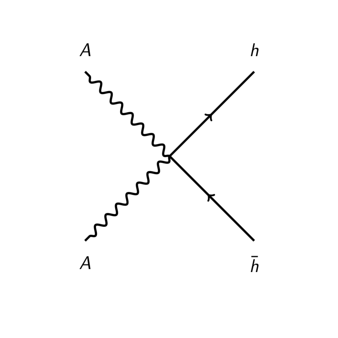
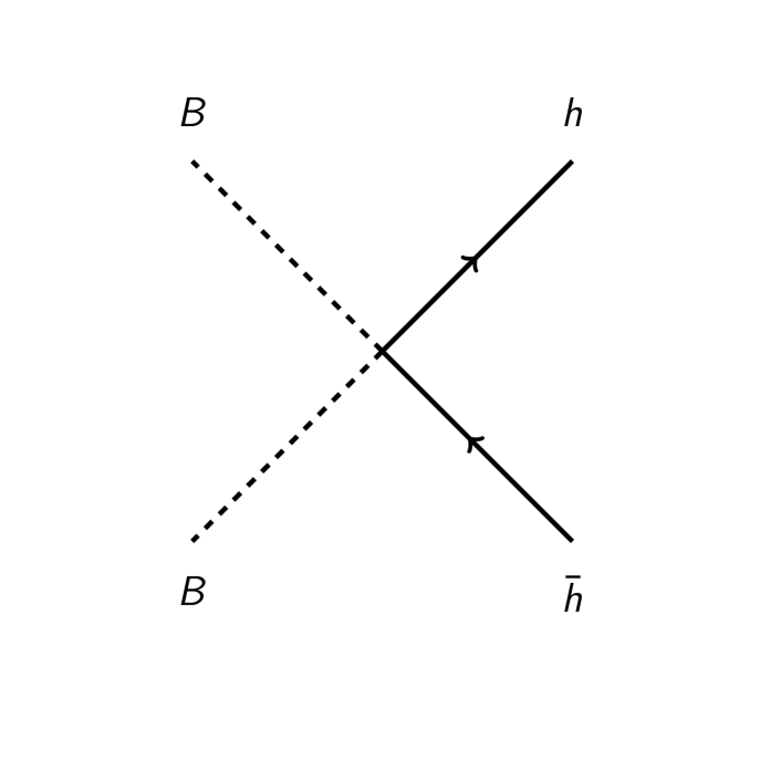
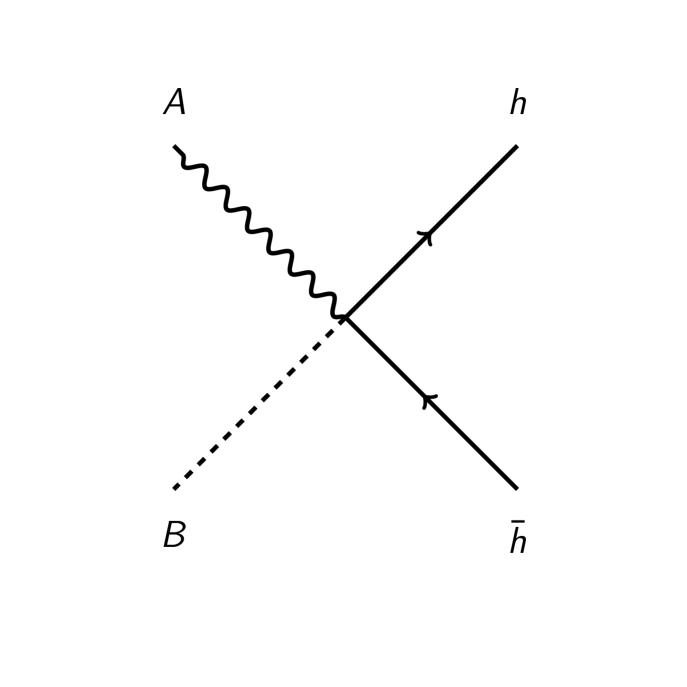
For example, Fig. (1(a)) describes $A+A\to h^{\dagger}+h$. Assuming large values of $s$, the center of mass energy, the cross section can be calculated in analogy to a Breit-Wheeler process in QED.

The total cross section for the processes in figure (1), under the same assumptions, are

	$\displaystyle\sigma(AA\to h^{\dagger}h)$	$\displaystyle=$	$\displaystyle\frac{g_{A}m_{h}}{s}\ln\left(\frac{\sqrt{s}}{m_{h}}\right)$
	$\displaystyle\sigma(BB\to h^{\dagger}h)$	$\displaystyle=$	$\displaystyle\frac{g_{B}m_{h}}{s}\ln\left(\frac{\sqrt{s}}{m_{h}}\right),$
	$\displaystyle\sigma(AB\to h^{\dagger}h)$	$\displaystyle=$	$\displaystyle\frac{g_{AB}m_{h}}{s}\ln\left(\frac{\sqrt{s}}{m_{h}}\right),$

implying the following cross sections ratios

	$\displaystyle\frac{\sigma(AA\to h^{\dagger}h)}{\sigma(BB\to h^{\dagger}h)}$	$\displaystyle=$	$\displaystyle\frac{g_{A}}{g_{B}},$
	$\displaystyle\frac{\sigma(AA\to h^{\dagger}h)}{\sigma(AB\to h^{\dagger}h)}$	$\displaystyle=$	$\displaystyle\frac{g_{A}}{g_{AB}},$		(34)
	$\displaystyle\frac{\sigma(BB\to h^{\dagger}h)}{\sigma(AB\to h^{\dagger}h)}$	$\displaystyle=$	$\displaystyle\frac{g_{B}}{g_{AB}}.$

Ratios (34) are simpler and more accessible in a model like the one we have discussed here.

The description of gauge theories with kinetic and magnetic mixing is an approach that has been intensively investigated in recent years as a way of describing dark matter. If magnetic mixing is included in the hidden sector, the possibility of seeing a millicharge effect would be possible.

In order to estimate the effects of millicharges one can proceed as follows: in section II we have seen that the presence of magnetic monopoles in the hidden sector induces the visible charge density (14) which can be interpreted as the millicharge (n=1)

$$q_{\mbox{\tiny{milli}}}=\frac{2\theta}{q_{\mbox{\tiny{B}}}}\frac{1}{1-\chi^{2}}\approx\frac{2\theta}{q_{\mbox{\tiny{B}}}},$$

(35)

which is a contribution due entirely to magnetic mixing.

The force produced by a millicharge compared to the Coulomb force between two electrons is

$$\left|\frac{F_{\mbox{\tiny{milli}}}}{F_{\mbox{\tiny{Coulomb}}}}\right|\approx\left(\frac{2\theta}{eq_{\mbox{\tiny{B}}}}\right)^{2},$$

while the force between an electron and a millicharge compared to the Coulomb force between two electrons is

$$\left|\frac{F_{\mbox{\tiny{milli}}-e}}{F_{\mbox{\tiny{e-e}}}}\right|\approx\frac{2\theta}{eq_{\mbox{\tiny{B}}}},$$

and the effects of the millicharges cannot be neglected.

The estimation of $\theta$ is central to cold dark matter phenomenology because the measurement of $\theta$ is an indirect measure that can be associated with axion detection via the Peccei-Quinn mechanism. Thus, the problem of estimating $\theta$ is moved to exploring the values of $g/M^{2}$ in axion phenomenology axionrev .

In this paper we have proposed an extension of the kinetic mixing idea to antisymmetric fields which could have implications in the search for physics beyond the standard model. Indeed, we have shown that this procedure gives rise to new decay channels. From here it is possible, in principle, to extract bounds for the coupling constants. Thus, antisymmetric fields can also be seen as another way of describing fundamental fields as was discussed long ago by Deser and Townsend (see deser ).

We would like to thank Prof. Fidel A. Schaposnik for interesting discussions in the initial stages of this work. This research was partially supported by Dicyt 042131GR (J.G.) and 041931MF (F.M.) and by Fundacion ONCE with grant Oportunidad al Talento (J.L.S.).

References

- (1) K. Hayashi, Phys. Lett. B 44 (1973), 497-501 doi:10.1016/0370-2693(73)90007-5
- (2) M. Kalb and P. Ramond, Phys. Rev. D 9 (1974), 2273-2284.
- (3) O. Cata and A. Ibarra, Phys. Rev. D 90 (2014) no.6, 063509 doi:10.1103/PhysRevD.90.063509.
- (4) S. Deser, Phys. Rev. 187 (1969), 1931-1934 doi:10.1103/PhysRev.187.1931; D. Z. Freedman and P. K. Townsend, Nucl. Phys. B 177 (1981), 282-296 doi:10.1016/0550-3213(81)90392-8; F. Quevedo and C. A. Trugenberger, Nucl. Phys. B 501 (1997), 143-172 doi:10.1016/S0550-3213(97)00337-4; P. K. Townsend, Phys. Lett. B 90 (1980), 275-276 doi:10.1016/0370-2693(80)90740-6.
- (5) F. Brümmer, J. Jaeckel and V. V. Khoze, JHEP 06 (2009), 037; F. Brümmer and J. Jaeckel, Phys. Lett. B 675 (2009), 360-364.
- (6) This method was developed several years ago in J. L. Cortes, J. Gamboa and L. Velazquez, Nucl. Phys. B 392 (1993), 645-666; ibid, Phys. Lett. B 286 (1992), 105-108.
- (7) B. Holdom, Phys. Lett. B 166 (1986), 196-198.
- (8) E. Witten, Phys. Lett. B 86 (1979), 283-287
- (9) P. A. M. Dirac, Phys. Rev. 74 (1948), 817-830.
- (10) T. T. Wu and C. N. Yang, Phys. Rev. D 12 (1975), 3843-3844.
- (11) For a review of monopoles see, P. Goddard and D. I. Olive, Rept. Prog. Phys. 41 (1978), 1357.
- (12) P. Orland, Nucl. Phys. B 205 (1982), 107-118.
- (13) C. Teitelboim, Phys. Lett. B 167 (1986), 63-68.
- (14) M. Del Zotto, J. J. Heckman, P. Kumar, A. Malekian and B. Wecht, Phys. Rev. D 95 (2017) no.1, 016007.
- (15) R. Nepomechie, Phys. Rev D 31, 1921 (1985).
- (16) C. Teitelboim, Phys. Lett. B 167 (1986), 69-72.
- (17) P. Orland, Nucl. Phys. B 205 (1982), 107-118.
- (18) M. Henneaux and C. Teitelboim, Found. Phys. 16 (1986), 593-617.
- (19) For recents reviews see; K. Abe et al. [XMASS], Phys. Lett. B 787 (2018), 153-158; S. Chaudhuri, K. Irwin, P. W. Graham and J. Mardon, [arXiv:1803.01627 [hep-ph]].; N. Vinyoles, A. Serenelli, F. L. Villante, S. Basu, J. Redondo and J. Isern, JCAP 10 (2015), 015.