Kinetic turbulence in fast 3D collisionless guide-field magnetic reconnection

Magnetic reconnection is a fundamental process that converts magnetic energy into kinetic energy and heat in laboratory, space and astrophysical plasmas Yamada et al. (2010); Treumann and Baumjohann (2013). Though ubiquitous in the collisionless plasmas of the Universe, it is not clear, yet, whether and which turbulence can enhance the energy conversion by reconnection. In the past it has been conjectured that macroscopic (fluid) turbulence can enhance the reconnection rate Matthaeus and Lamkin (1985); Lazarian and Vishniac (1999). But the role of kinetic turbulence in collisionless magnetic reconnection is much less explored. Indeed, as is well known, current sheets (CSs), through which magnetic reconnection takes place, contain a sufficient amount of free energy which in collisionless plasmas is released by instabilities at the smallest, kinetic scales. In contrast to fluid (magnetohydrodynamics, MHD) turbulence, the universality and properties of collisionless turbulence self-generated by magnetic reconnection, such as their scaling, power law spectral index and spectral breaks, are not yet well understood.

Recent in-situ measurements often detected thin current sheets formed in the turbulent space plasmas of the solar wind or Earth’s magnetosheath, leading to magnetic reconnection events generating heating and dissipation Retinò et al. (2007); Sundkvist et al. (2007); Gosling (2012); Perri et al. (2012); Osman et al. (2014); Wang et al. (2015); Osman et al. (2015); Chasapis et al. (2015); Vörös et al. (2016); Yordanova et al. (2016). The small-scale turbulence in the vicinity of those CSs can usually be associated to spectral breaks in the magnetic fluctuation spectra near the ion cyclotron frequency $\Omega_{ci}$. At larger scales (low frequencies), there is the characteristic inertial range of the turbulent cascade, while above ion scales the turbulent spectra shows a clear power law with spectral indices close to $-2.7$ Eastwood et al. (2009); Huang et al. (2012). However, the power-laws and spectral breaks near CSs are very similar to those measured in homogeneous turbulent solar wind plasmas Alexandrova et al. (2009); Eastwood et al. (2009); Chen et al. (2013), and that is why it is not well known how much reconnection contributes to the measured spectra. In addition, the spectral breaks might not be universal and depend on several parameters Chen et al. (2014a); Bourouaine et al. (2012); Bruno and Trenchi (2014); Boldyrev et al. (2015); Breuillard et al. (2016). Note that similar spectra, but with different spectral indices, were also obtained for other quantities such as the electric field Bale et al. (2005); Chen et al. (2011); Mozer and Chen (2013); Matteini et al. (2016), density Chen et al. (2012, 2014b); Šafránková et al. (2015) and higher order momenta of the distribution functions such as bulk flow velocity and temperature Podesta et al. (2006); Šafránková et al. (2013, 2016). On the other hand, laboratory experiments of magnetic reconnection (MRX, VTF, Vineta-II) obtained turbulent cascades as well but with different spectral indices and spectral breaks near the lower-hybrid frequency $\Omega_{LH}=\omega_{pi}/\sqrt{1+\omega_{pe}^{2}/\Omega_{ce}^{2}}$ (where $\omega_{pe}$ ($\omega_{pi}$) is the electron (ion) plasma frequency and $\Omega_{ce}$ is the electron cyclotron frequency) Carter et al. (2002); Fox et al. (2010); von Stechow et al. (2015). These different spectral breaks indicate a change in the physical nature of turbulence, depending only on the ions (in space plasmas) or with an influence of the electrons (in laboratory plasmas). In space, the first spectral break observed in steady and homogeneous solar wind turbulence is usually explained by a turbulent cascade of kinetic Alfvén waves (KAW) Leamon et al. (1999); Passot and Sulem (2015), whistler waves Stawicki et al. (2001), Landau damping Leamon et al. (1999); Howes et al. (2008a); Boldyrev et al. (2013), ion cyclotron damping Gary (1999) or combinations of these mechanisms depending on parameters such as the plasma-$\beta$ Boldyrev et al. (2015). There is even some evidence from measurements of homogeneous turbulence in the solar wind of a second spectral break near electrons scales and a steeper power law spectral index beyond it Sahraoui et al. (2009, 2013); Huang et al. (2014). However, measurements at those high electron frequencies are more difficult to obtain due to the instrumental limitations, and other interpretations such as an exponential cutoff beyond electron scales have also been proposed Alexandrova et al. (2009).

It is important to mention, however, that all those spectra measurements in space plasmas are performed in the spacecraft frame of reference, which gives a Doppler-shifted frequency $\omega_{sc}=\omega+\vec{k}\cdot\vec{v}_{sw}$, where $\vec{v}_{sw}$ is the plasma flow (solar wind) speed. In order to compare with theoretical predictions in the plasma frame of reference, a transformation has to be carried out to the wavenumber domain $\vec{k}$ by assuming the validity of Taylor’s hypothesis Taylor (1938) $\omega\ll\vec{k}\cdot\vec{v}_{sw}$. This implies a linear relationship between the spacecraft frequency space and the wavenumber domain in the plasma frame $k=\omega_{sc}/(|v_{sw}|\cos\theta)$, while the frequency spectrum in the plasma frame $\omega$ remains unknown. In the last expression, $\theta$ is the angle between the wavenumber $\vec{k}$ and solar wind velocity $\vec{v}_{sw}$, i.e., $\vec{k}\cdot\vec{v}_{sw}=k|\vec{v}_{sw}|\cos\theta$. This hypothesis is not valid for slow plasma flows or for high frequency dispersive waves with a non-linear relation with the wavenumber Klein et al. (2014, 2015).

Another important point related to terminology is that electron scales in spacecraft measurements have a slightly different meaning than in a pure frequency analysis in the plasma frame. This is because it refers to the wavenumber $kd_{e}$ (electron skin depth) mapped to the frequency space by using the previously discussed Taylor’s hypothesis, resulting in $\omega_{de}=v_{sw}/d_{e}$. This frequency is closer to the corresponding ion scales $\omega_{di}=v_{sw}/d_{i}$ (mapping of the wavenumber related to the ion skin depth $kd_{i}$) by a factor of the square root of the mass ratio $\sqrt{m_{i}/m_{e}}$ (also valid for the electron (ion) gyroradius $k\rho_{e}$ ($k\rho_{i}$)) compared to a direct frequency spectra, where the ion and electron frequencies $\Omega_{ci}$ and $\Omega_{ce}$ are separated by $m_{i}/m_{e}$.

The properties of stationary and homogeneous kinetic turbulence leading to localized magnetic reconnection were numerically investigated using hybrid-PIC (Particle-in-Cell), gyrokinetic or Vlasov codes simulations Howes et al. (2008b); Parashar et al. (2009); Greco et al. (2012); Valentini et al. (2014); Franci et al. (2015); Servidio et al. (2015); Navarro et al. (2016); Parashar and Matthaeus (2016); Cerri and Califano (2017); Franci et al. (2017). These investigations showed that ion-scale CSs, where magnetic reconnection can take place, can form from decaying or driven turbulence, leading to heating, temperature anisotropies and dissipation. Fully-kinetic PIC code simulations of shear-driven or decaying turbulence demonstrated that CSs also form at electron scales and contribute to the turbulent spectra Wan et al. (2012); Wu et al. (2013); Karimabadi et al. (2013); Haynes et al. (2014); Wan et al. (2015); Grošelj et al. (2018). A recent comparison of shear-driven turbulence with different physical and numerical models also showed the formation of current sheets and hinted towards the importance of reconnection in turbulence at different scales Grošelj et al. (2017). The idea that magnetic reconnection can have an important contribution to turbulence has also been suggested by a number of recent theoretical works in both collisional and collisionless regimes Howes (2015); Mallet et al. (2017a, b); Loureiro and Boldyrev (2017a, b); Boldyrev and Loureiro (2017) (see also the review Matthaeus et al. (2015)). In spite of all those works assessing the role of multiple magnetic reconnection events in turbulence, the opposite problem of the turbulence generated by magnetic reconnection in a single isolated current sheet has been rarely characterized. Although there has been some work analyzing the turbulence generated by plasmoid magnetic reconnection within the MHD framework Huang and Bhattacharjee (2016), the self-generated turbulence due to kinetic instabilities in collisionless magnetic reconnection is much less known. For example, Leonardis et al. (2013) is one of the few studies analyzing this problem using 3D fully-kinetic PIC-code simulations of reconnection, revealing the presence of non-Gaussian statistics and multifractal structures associated with intermittency and dissipation. Note that all these simulations usually revealed the spatial turbulence spectra, while the also relevant frequency spectrum have remained mostly unknown, which is one of the purposes of this study.

On the other hand, the properties of instabilities in CSs and their consequences for the kinetic turbulence generated during magnetic reconnection were also investigated by using 3D PIC-code Büchner and Kuska (1999) or fully-kinetic 3D Vlasov-code simulations Silin and Büchner (2003a, b). In particular, the role of Buneman instability was studied with Vlasov codes Büchner and Elkina (2005, 2006). This instability is relevant to understand the consequences of the self-generated turbulence in reconnection, because it can produce anomalous resistivity and thus balance the reconnection electric field associated to magnetic reconnection Che et al. (2011a); Che (2017). Even though in 2.5D fully-kinetic reconnection simulations this anomalous resistivity could not be found Muñoz et al. (2017), other 3D fully-kinetic reconnection simulations provided some positive evidence Drake et al. (2003); Che et al. (2011a); Liu et al. (2013); Price et al. (2016, 2017).

Although we do not attempt to make a direct comparison with spacecraft measurements or check the validity of Taylor’s hypothesis under realistic conditions, the need to study the properties of both the frequency and wavenumber spectra at kinetic and dispersive scales generated by magnetic reconnection is clear. In collisionless plasmas, the high-frequency kinetic turbulence is essential for the balance of electric fields, and therefore for the rate of magnetic reconnection, for energy dissipation and heating Büchner (2007).

We investigated the kinetic turbulence, self-generated in 3D collisionless reconnection, and its consequences for the reconnection rate, considering force-free equilibrium current sheets. Those are closer to real and astrophysical CSs rather than Harris-type CS, which require strong pressure gradients. In force-free CSs with a guide field in the current (our $z$-) direction, the magnetic pressure is balanced by an electron shear flow in the $x$ direction, while the thermal pressure is constant (see specific setup in Muñoz et al. (2015)). We used the 3D fully-kinetic PIC-code ACRONYM Kilian et al. (2012). We illustrate our findings by presenting the results of a simulation run with an ion to electron mass ratio $m_{i}/m_{e}=100$, initially equal electron and ion temperatures ($T_{i}/T_{e}=1.0$), a plasma beta $\beta_{e}=\beta_{i}=2\mu_{0}n_{0}k_{B}T_{i}/B_{T}^{2}=0.016$, a ratio of the electron thermal speed to the speed of light of $v_{th,e}/c=0.1$ and a relative guide field strength $b_{g}=B_{g}/B_{\infty y}=2$, where $B_{\infty y}$ is the asymptotic magnetic field (often abbreviated here as $B_{0}$). The initial total magnetic field $B_{T}=B_{\infty y}\sqrt{1+b_{g}^{2}}$ is constant, as well as the ion and electron number densities $n_{0}=n_{i}=n_{e}$. Note that the plasma beta on the asymptotic magnetic field and guide fields are, respectively, $\beta_{e,B\infty y}=\beta_{i,B\infty y}=0.08$ and $\beta_{e,Bg}=\beta_{i,Bg}=0.02$. Here, $v_{th,e}=\sqrt{k_{B}T_{e}}/m_{e}$ ($v_{th,i}=\sqrt{k_{B}T_{i}}/m_{i}$), and therefore the electron (ion) Larmor radius on the total magnetic field is $\rho_{e}=v_{th,e}/\Omega_{ce,BT}=(\sqrt{k_{B}T_{e}}/m_{e})/(eB_{T}/m_{e})$ ($\rho_{i}=v_{th,i}/\Omega_{ci,BT}=(\sqrt{k_{B}T_{i}}/m_{i})/(eB_{T}/m_{i})$). This definition leads to a ratio of characteristic length scales $\rho_{i}/d_{e}=0.89$. The current sheet halfwidth is $L=0.25d_{i}$.

In the case further discussed here the number of particles per cell (ppc) was 200 (100 per specie), with a total of $2.7\cdot 10^{10}$ particles in the simulation box. The simulation box covers a domain $L_{x}\times L_{y}\times L_{z}=4\,d_{i}\times 8\,d_{i}\times 16\,d_{i}$, where $d_{i}=c/\omega_{pi}$ is the ion inertial length ($\omega_{pi}$ is the ion plasma frequency). The calculations were carried out on a mesh containing $256\times 512\times 1024$ grid points. Periodic boundary conditions were chosen since we simulated two equivalent but oppositely directed current sheet flows. For comparison with other studies of turbulence in the wavenumber domain, our system allows the following minimum and maximum value of wavenumbers: $k_{\parallel}d_{i}=[0.392-201]$ (or $k_{\parallel}\rho_{i}=[0.035-17.98]$), and $k_{\perp}d_{i}=[0.785-201]$ (or $k_{\perp}\rho_{i}=[0.07-17.98]$). Here $k_{\parallel}=k_{z}$ (out-of-reconnection-plane direction, because of the dominant guide field) and $k_{\perp}=k_{y}$ (along the reconnected component of the magnetic field).

Reconnection is triggered by an initial magnetic field perturbation with amplitude $0.07B_{\infty y}$ for the corresponding magnetic field components ($B_{x}$ and $B_{y}$). This perturbation is narrowly localized in the current direction around $z=L_{z}/2$ and with a long wavelength tearing mode in the $y$-direction, generating a three-dimensional X-point.

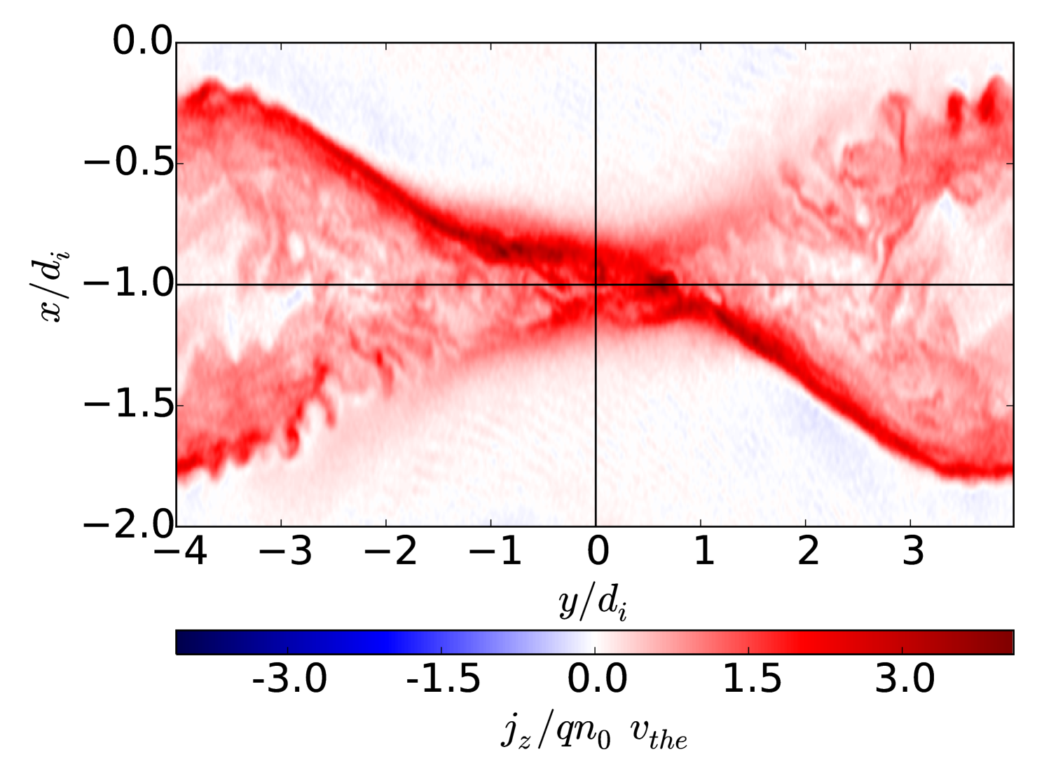
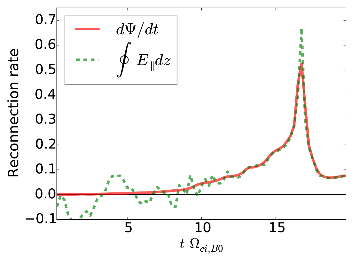
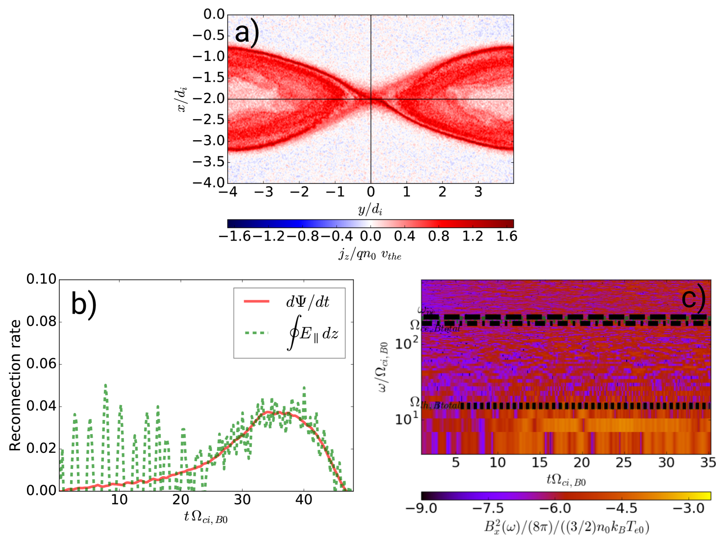
Fig. 1 depicts the spatial distribution of the current density distribution $j_{z}$ in the plane $z=L_{z}/2$ at $t=13.5\,\Omega_{ci}^{-1}$, after reconnection has fully developed. The Figure illustrates the well-known asymmetric structure of finite guide-field reconnection and the spatial structure of turbulence. Fig. 2 shows the reconnection rate numerically calculated in two different ways, which, by definition, should be identical, both characterizing the efficiency of reconnection. $d\psi/dt$ (red solid line) is the rate of change of the total magnetic flux calculated across a rectangle formed by the X and O lines of reconnection and the lines connecting $y=L_{y}/2$ and $y=0$. This quantity should be equal to $\oint E_{\parallel}dz$ (with $E_{\parallel}=\vec{E}\cdot\vec{B}/B$) represented with a green dashed line, the parallel electric field integrated along the perimeter of the same rectangle. The deviation between the two quantities is due to numerical errors caused by the PIC-code shot noise, which affects more the determination of the electric field rather than other quantities. As Fig. 2) illustrates, reconnection starts to grow significantly only after $t\sim 10\,\Omega_{ci}^{-1}$, reaches the limit of fast Petschek reconnection (0.1 in normalized units) at $t\sim 13\,\Omega_{ci}^{-1}$, and further grows doubling that rate by $t=15\,\Omega_{ci}^{-1}$. But the peak at $t=16.5\,\Omega_{ci}^{-1}$, with values of the reconnection rates as high as $0.5V_{A}B_{\infty y}$, is not due to only reconnection at the X-line, but also due to the effects of the periodic boundary conditions: the second current sheet starts to interact with the first current sheet (the one studied here). One effect of this is that the boundary of the magnetic island of the second current sheet is next to the X-line of the first one, limiting their growth and causing strong instabilities at the contact points due to the counterstreaming flows and possibly secondary reconnection sites. A second effect is that the available magnetic flux incoming to each current sheet is drastically reduced, throttling the reconnection rates by a large amount. In particular, the latter effect can be seen after $t\approx 16.5\Omega_{ci}^{-1}$ in Fig. 2, displaying a sharp decrease in the reconnection rates to values below 0.1 $V_{A}B_{\infty y}$. By $t\approx 18\Omega_{ci}^{-1}$ all the available magnetic flux is already exhausted and after $t\approx(20-21)\Omega_{ci}^{-1}$ reconnection stops. Because of this, all the processes after $t\approx 15\Omega_{ci}^{-1}$ should already be affected by the direct interaction between the two current sheets and are not representative of single X-line reconnection. Note that the described evolution of reconnection in this system is dependent on the simulation box size, especially along the current direction ($z$). The reconnection onset and peak values of the reconnection rate are reached later for longer boxes and the whole reconnection process is longer if the system is long enough along the current direction.

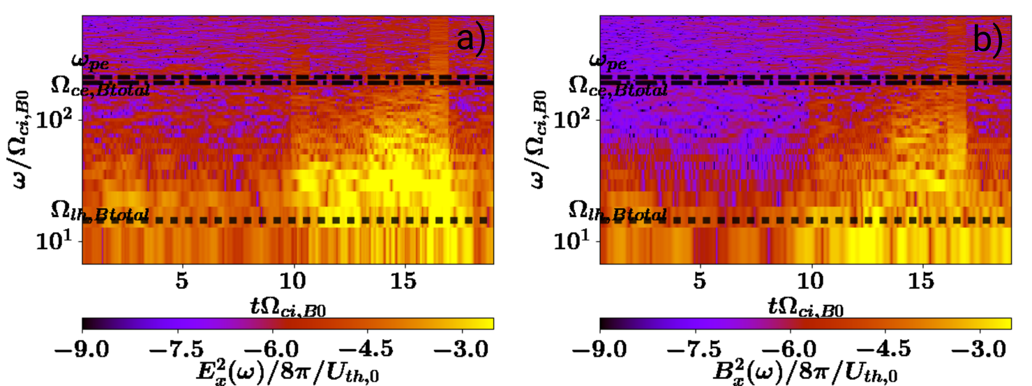
The dynamic spectrum of the turbulence is depicted by Figs. 3, which show the temporal evolution of the frequency spectrum of electric and magnetic fields in the direction perpendicular to the current flow direction at the X-point of reconnection. We obtained them by a short-time Fourier transform using a sliding Tukey window with an appropriate overlap and plotted as spectrograms. Figs. 3 shows that until about $t=10\,\Omega_{ci}^{-1}$, significant turbulence is developed only below the lower-hybrid frequency $\Omega_{LH}$. After that time both electric and magnetic turbulence strongly increase at kinetic scales up to the electron frequencies. The turbulence broadening correlates well with the enhanced reconnection rates (cf. Fig. 2).

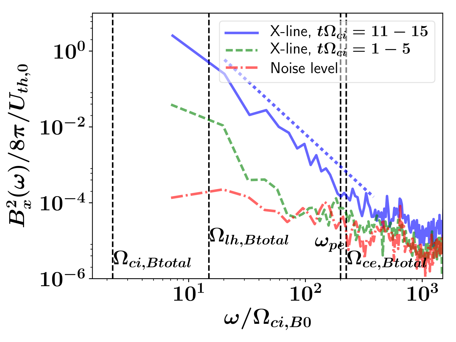
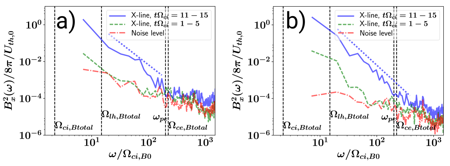
In Fig. 4, we show the resulting frequency spectra of the perpendicular magnetic field fluctuations $B_{x}$ at the X-line during two different characteristic time intervals: $t\,\Omega_{ci}=1-5$ and $t\,\Omega_{ci}=11-15$. In order to diminish the noise level, we bin the raw simulation data and averaging every eight data points (for both frequency and spectral power). This is equivalent to an average over an interval of $14\,\Omega_{ci,B0}$. Note that by binning the simulation data, the minimum resolved frequency becomes larger, and closer to the lower-hybrid frequency $\Omega_{LH}$. But it does not modify the spectral slope above $\Omega_{LH}$, which is our main interest here.

The comparison of these two spectra at the intervals $t\,\Omega_{ci}=1-5$ and $t\,\Omega_{ci}=11-15$ clearly demonstrates the development of the high-frequency kinetic scale turbulence above the lower-hybrid frequency but also an enhanced spectral power close to $\Omega_{LH}$. Note that Fig. 4 also shows the spectrum of the (numerical) shot noise of the magnetic fluctuations (red dashed line) due to the finite number of particles used in the PIC-code simulations. This noise spectrum was obtained at a location away from the CSs. The plot indicates that fluctuations at frequencies above $\omega_{pe}$ and $\Omega_{ce}$ (more specifically, above $\omega\gtrsim 400\,\Omega_{ci,B0}$), shown as dashed vertical lines, are due to numerical effects, while the turbulence below these electron frequencies significantly exceeds the numerical noise level. Above $\Omega_{LH}$, however, a clear steep power law spectrum $P=\omega^{\alpha}$ develops, with a spectral index $\alpha\approx-2.83$ which extends up to the electron frequencies $\omega_{pe}$ and $\Omega_{ce}$. More precisely, we calculated the spectral index by means of a least squares linear fit in the frequency range $\omega/\Omega_{ci,B0}=17-400$ (for the interval $t\,\Omega_{ci}=11-15$), in order to consider all the frequency range above $\Omega_{LH}$ until the numerical noise level. This reference spectral slope and its associated range is indicated as a dashed blue continuous line in Fig. 4. See Appendix A for a discussion about the effects of the particle number and the choice of frequency range for the fitting on those results.

Note that in contrast to the usually used simpler spatial structure analysis of the turbulence, we used a direct time-frequency-domain diagnostic of high cadence simulation data by a stationary virtual probe located at the X-point of reconnection, which provides the simplest and most general way of analyzing the frequency turbulent spectra in this system. This approach provides different insights in those kind of simulations, while related work by Dmitruk and Matthaeus (2009); TenBarge and Howes (2012) analyzed the frequency spectra in homogeneous turbulence simulations. Although this spectral index $-2.8$ is often measured by spacecrafts in turbulent space plasmas undergoing reconnection between ion and electron scales (roughly the frequency-mapped $kd_{i}$ to $kd_{e}$ by assuming Taylor’s hypothesis) Eastwood et al. (2009); Wang et al. (2015), a direct comparison is not appropriate, because the spacecrafts are always in relative motion with respect to the plasma frame. Instead, our method to obtain frequency spectra actually compares better with laboratory experiments, where their probes are stationary. Furthermore, the compared range is not the same between simulations and space observations: the lower hybrid frequency is usually above the typical frequency range accessible by space instruments, since it approximately coincides with the location of the second spectral break (at the frequency-mapped $kd_{e}$) if the frequency mapped $kd_{i}$ is close to $\Omega_{ci}$ Sahraoui et al. (2009, 2013); Huang et al. (2014). Nevertheless, this range of frequencies is more easily accessible in laboratory experiments, which reveal a spectral break and a steep power law above $\Omega_{LH}$ Carter et al. (2002); Fox et al. (2010); von Stechow et al. (2015).

Note that it is important to obtain independently both frequency and wavenumber spectra of fluctuations in order to get the plasmas dispersive properties without any preliminary assumption such as Taylor’s hypothesis, which might not apply for high-frequency dispersive waves, as in our simulations. In view of this, we also calculated the spatial spectra in our simulations. Thus, we can make a proper comparison with our resulting frequency spectra, as well as to previous studies and observations or measurements.

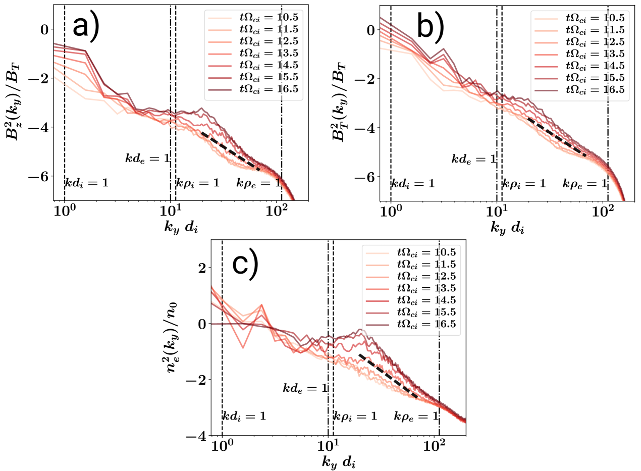
The results for the calculation of the wavenumber spectra at the center of the left CS $x=-1.0d_{i}$ and along the $y$ direction are shown in Figs. 5. These figures show the power spectral density (PSD) of the fluctuations in the parallel magnetic field $B_{z}^{2}(k_{y})$ (a) total magnetic field $B_{T}^{2}(k_{y})=B_{x}^{2}(k_{y})+B_{y}^{2}(k_{y})+B_{z}^{2}(k_{y})$ (b), and electron density $n_{e}^{2}(k_{y})$ (c). Each wavenumber spectra is averaged along the out-of-plane direction $z$. Common features for the magnetic field and density spectra are the monotonously increasing spectral power as the times goes by, a bump beyond $k=\rho_{i}^{-1}$ (more precisely, at $kd_{i}\sim 20$), in particular for $\delta n_{e}$ and $\delta B_{T}$, and a numerical steepening close to the grid scales for $k\rho_{e}>1$.

Between $k\rho_{i}=1$ and $k\rho_{e}=1$, there are some ranges where a straight line can be fitted. Therefore, we calculate spectral slopes $\alpha$ using a least squares linear fit of $P=k^{\alpha}$ for all the available wavenumber data in a given range. It is clear from Figs. 5 that those $k$-spectral indices are dynamical quantities depending on time, loosely correlated with the value of the reconnection rate. For reference, we indicate by a black dashed line the reference slope -2.8 close to the spectra obtained at $t\Omega_{ci}=13.5$. The plots demonstrate a good fit in the wavenumber range $kd_{i}=20-80$. For earlier times, the range for the linear fitting is moved to smaller wavenumbers, $kd_{i}=10-35$, because there is a clear flattening of the spectra at about $kd_{i}\sim 40$, in particular of the $B_{z}$ component of the magnetic field fluctuations. For late times ($t\Omega_{ci}\gtrsim 13.5$), we use the wavenumber range $kd_{i}=20-80$ for the linear fitting, since this includes the wavenumbers above the bump beyond $k\rho_{i}\geq 1$, where the spectra corresponds to a straight line.

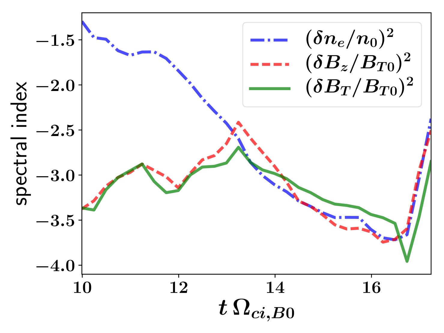
The variation of the spectral indices with time is summarized by the Fig. 6. This Figure shows that the slope of the electron density fluctuations continuously steepens with time (see also Fig. 5c), reaching a maximum of $\alpha\approx-3.7$ at $t\Omega_{ci}\approx 16.5$. At this time the reconnection rate is maximum until it becomes determined by the interaction of the two current sheets in the simulation domain. Meanwhile, the parallel and total magnetic field fluctuations flatten until $t\Omega_{ci}\approx 13.2$. Later they steepen again, with similar spectral indices, and are also comparable in power to the electron density fluctuations. Close to $t\Omega_{ci}\approx 13.2$, the spectral indices reach the range $\alpha=[-2.8,-2.5]$. At this same time, the normalized reconnection rate becomes $0.1$ (c.f. Fig. 2). The spectral indices become $\alpha=[-3.5,-3.3]$ at $t\Omega_{ci}\approx 15$, where the energy conversion rate is $\sim 0.2$ (normalized reconnection rate), before reconnection becomes affected by the second current sheet in the simulation domain at $t\Omega_{ci}\approx 16.5$.

Therefore, the varying value of these spectral index slopes in the wavenumber domain probably indicates that the kind of turbulence developed due to non-steady reconnection, dominated by instabilities, also changes during the course of reconnection.

We also analyzed the wavenumber spectra of density and magnetic fluctuations along the out-of-plane direction $z$ (mostly aligned with the dominant guide field) in the region near the X-line. A similar analysis also reveals a power law spectra with similar variable spectral indices (and in approximately the same range). Those wavenumber spectra, however, do not show a clear spectral break near $k\rho_{i}=1$ and they also display a shorter turbulent cascade when no spatial average is used (plots not shown here), since the noise level is higher. Note that if an average of the wavenumber spectra in $k_{z}$ along the current sheet ($y$ direction) would be performed, it would make to distinguish and fit a power law more difficult, since the inhomogeneity and general features of turbulence in the outflow region are very different from those near the X-line, averaging out different kind of processes. In contrast, an average of the power spectral in $k_{y}$ along $z$ (the one used here) is more consistent because it is similar among different slices.

The spatial spectral indices of the self-generated magnetic turbulence along the CS are similar to those measured in space plasmas close to $\alpha=-2.7$, but only when the (normalized) reconnection rates are close to 0.1. Those spectral indices in the wavenumber domain are also within the same range as the frequency spectral slope measured here for a stationary probe at the X-point (see Fig. 4). However, this similar slope in $\omega$ and $k_{y}$ does not necessarily indicate the presence of non-dispersive waves with a linear dependence between $\omega$ and $k_{y}$, since we verified that the $\omega$-spectrum is different in the outflow regions of reconnection: far from the X-line, there are less turbulence and, therefore, the magnetic frequency spectrum does not develop a spectral index as steep as in the X-line. Since the $k_{y}$ spectrum considers equally all these regions with different properties in the $\omega$ domain, a dispersion relation $\omega$ - $k_{y}$ cannot be inferred uniquely from a single sampling point in time. Moreover, based on different 2D simulations for a similar parameter range (with a higher output cadence), dispersion relations $\omega$ - $k_{y}$ hint to the presence of dispersive waves in the whistler branch with a quadratic dependence $\omega\propto k_{y}^{2}$. Nevertheless, more work is needed to clarify if the similarity of $\omega$ and $k_{y}$ spectral indices is the result of our parameter range or a more generic characteristic of this kind of turbulent system.

One of the goals of other works analyzing the turbulence at kinetic scales is identifying whether the turbulent fluctuations can be classified as due to KAWs or whistler waves Chen et al. (2013); Boldyrev et al. (2013); Cerri et al. (2016). The identification criteria is based on asymptotic formulas leading to dispersion relations and associated transport ratios related to the compressibility of fluctuations. However, those expressions require $\omega\ll k_{\perp}v_{th,i}$ for KAWs and $k_{\perp}v_{th,i}\ll\omega\ll k_{z}v_{th,e}$ for whistler waves (see Fig. 1 of Ref. Boldyrev et al., 2013), which are not well satisfied in our case. One of the most important reasons is that many of those formulas are derived for conditions $\beta\sim 1$, which do not apply well in our simulations with small plasma-$\beta$, in addition to the use of an artificially small mass ratio and simulation domain sizes.

The broadband turbulence at the X-line self-generated by reconnection, enhancing the spectral power between the lower hybrid and electron frequencies, is caused mainly by a (streaming) Buneman instability Buneman (1958). The source of free energy of this instability is the relative streaming of the current-carrying electrons with respect to the ions. We verified this conjecture by investigating the evolution of the drift speed $V_{rel,z}$ along the X-line of reconnection, with $V_{rel,z}=V_{i,z}-V_{e,z}$, where $V_{i,z}$ ($V_{e,z}$) is the ion (electron) drift speed along $z$. As one can see in Fig. 7a), initially, in the thin CS $V_{rel,z}$ already slightly exceeds the initial electron thermal speed $v_{th,e}$. This causes an initial (parallel) plasma heating, i.e., the electron thermal speed $v_{th,e,z}$ increases. The marginal Buneman instability criterion $V_{rel,z}\sim v_{th,e,z}$, however, is not reached again until $t\sim 9\,\Omega_{ci}^{-1}$. This way $V_{rel,z}/v_{th,e,z}$ can again increase above the threshold of the Buneman instability. Exactly at that time the broadband kinetic turbulence starts to develop. After that the electron heating continues while the electron-ion drift speed now grows even faster than the electron thermal velocity. This keeps the CS Buneman-unstable until boundary effects starts to play a significant role close to $t\Omega_{ci}\sim 16.5$. Note that previous 3D magnetic reconnection studies reported similar Buneman-type instabilities and the generation of current filaments in the current density along the $z$ direction Drake et al. (2003); Che et al. (2011a). The Buneman streaming instability is not effective in 2.5D magnetic reconnection in which, therefore, no high-frequency turbulence near $\Omega_{LH}$ develops Muñoz and Büchner (2016).

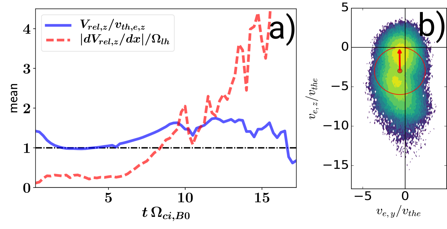
As a second contribution to the broadband kinetic turbulence, which also enhances reconnection, an electron shear flow instability is excited at the reconnection site. Fig. 7a) shows the gradient of the current-aligned electron flow across the CS, $dV_{e,z}/dx$. It strongly grows after $t\Omega_{ci}\gtrsim 13$ when it exceeds the threshold of the electron-ion hybrid (EIH) instability $dV_{e,z}/dx\gg\Omega_{LH}$ Ganguli et al. (1988); Romero et al. (1992). The EIH instability is a kinetic branch of the Kelvin-Helmholtz instability which enhances the plasma turbulence near the lower-hybrid frequency. The kinetic shear flow instability criterion is fulfilled, however, only after the Buneman streaming instability has already developed.

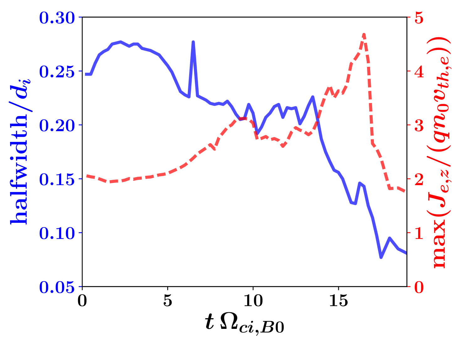
The most active period of both instabilities ($t\Omega_{ci}\gtrsim 13.5$), described above, it is also correlated with a fast thinning of the current sheet. Fig. 8 shows the evolution of the halfwidth and maximum of the electron current density $J_{e,z}$. We choose to diagnose this quantity and not $J_{z}$ because most of the current is carried by the electrons, both initially and also later during the course of the CS evolution. An ion current sheet also forms self-consistently, but its contribution to the total current is much smaller and it is also much broader. We calculate the quantities shown in Fig. 8 in the $x-y$ reconnection-plane along a cut in the $x$ direction through the center of the first current sheet ($y=0$). This is approximately the location of the X-point. We also average $J_{e,z}(x,y)$ along the out-of-plane direction $z$. Thus, the maximum value of the average $\bar{J}_{e,z}(x,y)$ is obtained from calculations along this cut as shown in Fig. 8 (the red line). On the other hand, we fit the function $f(x)=C+A\cosh^{-2}(x/\lambda)$ ($A$, $C$ and $\lambda$ are all fitting variables) to the same $x$-cut in order to get the halfwidth $\lambda$ of the electron current sheet. This quantity is shown in Fig. 8 by a blue line. Note that due to the averaging along the $z-$direction, the actual halfwidth of the current sheet at given $z$-slices can be smaller or larger than that value.

This way, Fig. 8 shows that the current sheet halfwidth quickly readjusts due to the initial perturbation and the lack of exact kinetic equilibrium of this force-free current sheet. Also, the initial current sheet is slightly Buneman unstable (c.f. Fig. 7). Later, when reconnection is laminar ($t\Omega_{ci}\lesssim 13.5$), the current sheet halfwidth does not change much away from $0.2d_{i}$. But during the non-linear evolution ($t\Omega_{ci}\gtrsim 13.5)$, when filaments appear, the reconnection rate is greatly enhanced and the spectral indices of the magnetic fluctuations grow beyond $-3.0$. Then, the halfwidth of the current sheet quickly decreases until it reaches values as low as $0.08d_{i}$. Meanwhile, the maximum $J_{e,z}$ grows steadily from the beginning, stays more or less constant during the period of laminar reconnection, to quickly grow, finally, during the nonlinear stage of reconnection.

Those instabilities and their turbulence also contributes to the generation of significant deviations in the electron velocity distribution function (EVDF) from the initial drifting Maxwellian. Beams are developed, temperature anisotropies and even a non-gyrotropy of the electron pressure tensor. This is illustrated in Fig. 7b), showing a cut through the EVDF in the plane $v_{y}-v_{z}$ obtained near the X-line of reconnection. A double peak is clearly visible in the EVDF, separated by about $4v_{th,e}$. It is due to the interaction of two counter-streaming beams, providing free energy for a two-streaming instability as well. The origin of those beams can be understood as follows. Originally, the electron distribution function is quite close to a shifted Maxwellian with a drift speed (along $z$) close to the electron drift speed, which is part of the initial conditions sustaining the current sheet. The reconnection dynamics pulls magnetic flux and thermal electrons (zero drift speed along $z$) from the upstream region into the X-line, bringing together those two populations with a relative drift speed between them. But reconnection also generates a reconnection electric field which accelerates electrons, forming a beam-like population with a very high drift speed and a non-thermal population as well. This also produces an elongated plateau in the $-v_{z}$ direction, which is a consequence of the non-linear evolution of the Buneman instability, leading also to beam-driven lower-hybrid instabilities McMillan and Cairns (2006, 2007), contributing to the turbulence near $\Omega_{LH}$.

Thus, while the beam-driven lower-hybrid instability is responsible mainly for the turbulence near the lower-hybrid frequency, Buneman and two-streaming instabilities are behind the high frequency kinetic turbulence. Since those instabilities should act simultaneously, it is not straightforward to disentangle their individual effects, considering also they should be mainly observed in their saturated state because of their large growth rate and their source of free energy continuously being supplied by magnetic reconnection. This high-frequency turbulence might also quickly change the shape of the EVDFs, but a detailed discussion about those effects is outside of the scope of this paper.

In our simulations, the presence of high-frequency kinetic turbulence is correlated with enhanced reconnection rates reaching $0.2V_{A}B_{\infty y}$ and up to $0.5V_{A}B_{\infty y}$. Although we did not prove a causal relationship, there is some evidence supporting that this association is not only a coincidence. First of all, as has been established for a long time, normalized reconnection rates close to 0.1 are typical for fast reconnection in Harris or force-free current sheets and within a wide range of parameters and physical models, more or less independent on the dissipation mechanism (see, e.g., Refs. Comisso and Bhattacharjee (2016); Liu et al. (2017); Cassak et al. (2017) and references therein). We found here, though, that the reconnection rate can be significantly enhanced by Buneman turbulence, similar to the findings of Che (2017). This can be interpreted as Buneman turbulence caused anomalous resistivity balancing the reconnection electric field in the framework of a generalized Ohm’s law. This requires relatively thin current sheets and fully 3D considerations. That is why such an enhanced reconnection rate was not commonly found in previous simulation studies, but it is within the parameter regime of our study. Therefore, the fact that Buneman instability is present in our simulations and reconnection rates are well above 0.1 hint towards the relation between reconnection rates and this kind of Buneman turbulence.

To support the relation between self-generated (mainly Buneman) turbulence and reconnection rate, we also simulated thicker current sheets (e.g., exactly the double: $L=0.5d_{i}$) for otherwise identical parameters. In order to keep the separation constant between the current sheets, we also increased the simulation box length across $x$ to twice its original value. We should mention that by changing the current sheet thickness we are also modifying the stability properties of this system, and so both simulation runs are not completely equivalent. It was found previously that the linear growth rates of the collisionless tearing mode are strongly reduced for thicker current sheets Pritchett et al. (1991); Brittnacher et al. (1995). In a just two times thicker current sheet the reduced magnetic field shear implies a relative electron-ion streaming speed below the threshold of the Buneman instability ($v_{th,e}$). As a consequence, no Buneman instability is triggered and the X-line does not become turbulent. This can be seen in Fig. 9a) displaying the out-of-plane current density $j_{z}$ at fully developed reconnection. Note that the onset of reconnection is delayed because of the thicker current sheet and the larger simulation box size. Fig. 9b) shows that reconnection rates are strongly reduced, with their peak value close to $0.05B_{\infty y}V_{A}$. This reduction of the reconnection rate is associated with weaker magnetic fluctuations, as it can be seen in Fig. 9c) showing the spectrogram of the perpendicular magnetic field. Different from the original run (see Fig. 3), it is clear that there is no development of a turbulent cascade and the spectral power is not enhanced at all above the lower hybrid frequency $\Omega_{LH}$. This supports the conjecture that Buneman turbulence enhances reconnection.

We have analyzed the properties of self-generated kinetic turbulence by 3D guide field reconnection in both, frequency and wavenumber, domains. In the course of reconnection, the self-generated turbulence starts to grow near the lower-hybrid frequency. Later, a broadband spectrum above the lower-hybrid frequency and up to electron frequencies forms, exhibiting a power law with a spectral index of $\alpha\sim-2.8$. Different from previous investigations, we obtained this power-law spectrum of perpendicular magnetic fluctuations directly in the frequency domain for a stationary probe at the X-point of reconnection. For comparison purposes, we also analyzed the wavenumber spectra in the direction perpendicular to the magnetic field. This also reveals a power law spectra with a very similar spectral index of $\alpha\sim-2.8$ for $k>\rho_{i}^{-1}$, but only at times when the normalized reconnection rates are close to $0.1$. This wavenumber spectral slope further steepens correlated with enhanced reconnection rates above that value. It is also associated with a spectral break close to $k>\rho_{i}^{-1}$. The similar slope of the $\omega$ and $k_{y}$ spectra does not necessarily indicate the presence of non-dispersive waves with a linear dependence between $\omega$ and $k_{y}$: we verified that the $\omega$-spectrum is different in the outflow regions of reconnection. Those results cannot be directly compared with space observations, but some of the characteristics of this kinetic turbulence have some points in common, as well as with laboratory experiments.

The turbulence near the lower-hybrid frequency is due to kinetic instabilities driven by the streaming of the current carriers, the electrons, their beams, and shear flows. First the Buneman streaming instability starts and later a kinetic electron shear flow instability takes over. These two unstable modes might become coupled Che et al. (2011b). The period of maximum activity of those unstable waves correlates with a fast thinning of the current sheet. The sources of free energy (electron currents and shear flows) are typical for guide field reconnection. This is in contrast to the limiting case of antiparallel reconnection, where anisotropy-driven and pressure-gradient-driven instabilities prevail. Our results indicate that simulations of magnetic reconnection need to be three-dimensional to accurately describe the intrinsic 3D self-generated turbulence in a real physical current sheet: 2D setups cannot reproduce all the fluctuations and unstable waves seen in realistic environments.

We also provided some evidence that the high-frequency kinetic turbulence generated by streaming and shear flow instabilities is correlated with enhanced reconnection rates. Usually, $0.1V_{A}B_{\infty y}$ is considered to the be the rate of fast reconnection. However, we showed here that the rate of reconnection through collisionless thin current sheets can be enhanced up to $(0.2-0.5)V_{A}B_{\infty y}$ in the presence of Buneman instability. This was also found in a different study Che (2017).

By means of an additional simulation with a thicker current sheet, where Buneman instability is not excited, we showed that the consequent lack of high-frequency turbulence is correlated with weaker reconnection rates on the order of $0.05V_{A}B_{\infty y}$. A more concrete and causal proof of this statement would exceed the scope of this paper.

For larger ion to electron mass ratios and initially thicker current sheets, the properties of the dominant instabilities might change. It is very likely that a broadband kinetic turbulence will nevertheless be excited and affect the reconnection process, as laboratory experiments and in-situ observations have shown. Starting with the current space mission MMS Burch et al. (2016) as well as by upcoming new laboratory experiments like FLARE at Princeton, also higher (electron) frequency turbulence will become observable which might compare better with our simulation results.

References

- Yamada et al. (2010) M. Yamada, R. M. Kulsrud, and H. Ji, Reviews of Modern Physics 82, 603 (2010).
- Treumann and Baumjohann (2013) R. A. Treumann and W. Baumjohann, Frontiers in Physics 1, 1 (2013).
- Matthaeus and Lamkin (1985) W. H. Matthaeus and S. L. Lamkin, Physics of Fluids 28, 303 (1985).
- Lazarian and Vishniac (1999) A. Lazarian and E. T. Vishniac, The Astrophysical Journal 517, 700 (1999).
- Retinò et al. (2007) A. Retinò, D. Sundkvist, A. Vaivads, F. Mozer, M. André, and C. J. Owen, Nature Physics 3, 236 (2007).
- Sundkvist et al. (2007) D. Sundkvist, A. Retinò, A. Vaivads, and S. D. Bale, Physical Review Letters 99, 025004 (2007).
- Gosling (2012) J. T. Gosling, Space Science Reviews 172, 187 (2012).
- Perri et al. (2012) S. Perri, M. L. Goldstein, J. C. Dorelli, and F. Sahraoui, Physical Review Letters 109, 191101 (2012).
- Osman et al. (2014) K. T. Osman, W. H. Matthaeus, J. T. Gosling, A. Greco, S. Servidio, B. Hnat, S. C. Chapman, and T. D. Phan, Physical Review Letters 112, 215002 (2014), arXiv:1403.4590 .
- Wang et al. (2015) Y. Wang, F. S. Wei, X. S. Feng, X. J. Xu, J. Zhang, T. R. Sun, and P. B. Zuo, The Astrophysical Journal Supplement Series 221, 34 (2015).
- Osman et al. (2015) K. T. Osman, K. H. Kiyani, W. H. Matthaeus, B. Hnat, S. C. Chapman, and Y. V. Khotyaintsev, The Astrophysical Journal 815, L24 (2015), arXiv:1508.04179 .
- Chasapis et al. (2015) A. Chasapis, A. Retinò, F. Sahraoui, A. Vaivads, Y. V. Khotyaintsev, D. Sundkvist, A. Greco, L. Sorriso-Valvo, and P. Canu, The Astrophysical Journal 804, L1 (2015).
- Vörös et al. (2016) Z. Vörös, E. Yordanova, M. M. Echim, G. Consolini, and Y. Narita, The Astrophysical Journal Letters 819, L15 (2016), arXiv:1603.00328 .
- Yordanova et al. (2016) E. Yordanova, Z. Vörös, A. Varsani, D. B. Graham, C. Norgren, Y. V. Khotyaintsev, A. Vaivads, E. Eriksson, R. Nakamura, P.-A. Lindqvist, G. Marklund, R. E. Ergun, W. Magnes, W. Baumjohann, D. Fischer, F. Plaschke, Y. Narita, C. T. Russell, R. J. Strangeway, O. Le Contel, C. Pollock, R. B. Torbert, B. J. Giles, J. L. Burch, L. A. Avanov, J. C. Dorelli, D. J. Gershman, W. R. Paterson, B. Lavraud, and Y. Saito, Geophysical Research Letters 43, 5969 (2016).
- Eastwood et al. (2009) J. P. Eastwood, T. D. Phan, S. D. Bale, and A. Tjulin, Physical Review Letters 102, 035001 (2009).
- Huang et al. (2012) S. Y. Huang, M. Zhou, F. Sahraoui, A. Vaivads, X. H. Deng, M. André, J. S. He, H. S. Fu, H. M. Li, Z. G. Yuan, and D. D. Wang, Geophysical Research Letters 39, L11104 (2012).
- Alexandrova et al. (2009) O. Alexandrova, J. Saur, C. Lacombe, A. Mangeney, J. Mitchell, S. J. Schwartz, and P. Robert, Physical Review Letters 103, 165003 (2009).
- Chen et al. (2013) C. H. K. Chen, S. Boldyrev, Q. Xia, and J. C. Perez, Physical Review Letters 110, 225002 (2013), arXiv:1305.2950 .
- Chen et al. (2014a) C. H. K. Chen, L. Leung, S. Boldyrev, B. A. Maruca, and S. D. Bale, Geophysical Research Letters 41, 8081 (2014a).
- Bourouaine et al. (2012) S. Bourouaine, O. Alexandrova, E. Marsch, and M. Maksimovic, The Astrophysical Journal 749, 102 (2012).
- Bruno and Trenchi (2014) R. Bruno and L. Trenchi, The Astrophysical Journal 787, L24 (2014).
- Boldyrev et al. (2015) S. Boldyrev, C. H. K. Chen, Q. Xia, and V. Zhdankin, The Astrophysical Journal 806, 238 (2015), arXiv:arXiv:1507.00416v1 .
- Breuillard et al. (2016) H. Breuillard, E. Yordanova, A. Vaivads, and O. Alexandrova, The Astrophysical Journal 829, 54 (2016).
- Bale et al. (2005) S. D. Bale, P. J. Kellogg, F. S. Mozer, T. S. Horbury, and H. Reme, Physical Review Letters 94, 215002 (2005), arXiv:0503103 [physics] .
- Chen et al. (2011) C. H. K. Chen, S. D. Bale, C. Salem, and F. S. Mozer, The Astrophysical Journal 737, L41 (2011).
- Mozer and Chen (2013) F. S. Mozer and C. H. K. Chen, The Astrophysical Journal 768, L10 (2013).
- Matteini et al. (2016) L. Matteini, O. Alexandrova, C. H. K. Chen, and C. Lacombe, Monthly Notices of the Royal Astronomical Society 466, 945 (2017).
- Chen et al. (2012) C. H. K. Chen, C. S. Salem, J. W. Bonnell, F. S. Mozer, and S. D. Bale, Physical Review Letters 109, 035001 (2012), arXiv:1205.5063 .
- Chen et al. (2014b) C. H. K. Chen, L. Sorriso-Valvo, J. Šafránková, and Z. Němeček, The Astrophysical Journal 789, L8 (2014b).
- Šafránková et al. (2015) J. Šafránková, Z. Nemecek, F. Nemec, L. Prech, A. Pitna, C. H. K. Chen, and G. N. Zastenker, The Astrophysical Journal 803, 107 (2015).
- Podesta et al. (2006) J. J. Podesta, D. A. Roberts, and M. L. Goldstein, Journal of Geophysical Research 111, A10109 (2006).
- Šafránková et al. (2013) J. Šafránková, Z. Němeček, L. Prech, and G. N. Zastenker, Physical Review Letters 110, 025004 (2013).
- Šafránková et al. (2016) J. Šafránková, Z. Nemecek, F. Nemec, L. Prech, C. H. K. Chen, and G. N. Zastenker, The Astrophysical Journal 825, 121 (2016).
- Carter et al. (2002) T. A. Carter, M. Yamada, H. Ji, R. M. Kulsrud, and F. Trintchouk, Physics of Plasmas 9, 3272 (2002).
- Fox et al. (2010) W. Fox, M. Porkolab, J. Egedal, N. Katz, and A. Le, Physics of Plasmas 17, 072303 (2010).
- von Stechow et al. (2015) A. von Stechow, O. Grulke, and T. Klinger, Plasma Physics and Controlled Fusion 58, 014016 (2015).
- Leamon et al. (1999) R. J. Leamon, C. W. Smith, N. F. Ness, and H. K. Wong, Journal of Geophysical Research: Space Physics 104, 22331 (1999).
- Passot and Sulem (2015) T. Passot and P. L. Sulem, The Astrophysical Journal Letters 812, L37 (2015), arXiv:arXiv:1509.02839v1 .
- Stawicki et al. (2001) O. Stawicki, S. P. Gary, and H. Li, Journal of Geophysical Research 106, 8273 (2001).
- Howes et al. (2008a) G. G. Howes, S. C. Cowley, W. Dorland, G. W. Hammett, E. Quataert, and A. A. Schekochihin, Journal of Geophysical Research 113, A05103 (2008a).
- Boldyrev et al. (2013) S. Boldyrev, K. Horaites, Q. Xia, and J. C. Perez, The Astrophysical Journal 777, 41 (2013).
- Gary (1999) S. P. Gary, Journal of Geophysical Research: Space Physics 104, 6759 (1999).
- Sahraoui et al. (2009) F. Sahraoui, M. L. Goldstein, P. Robert, and Y. V. Khotyaintsev, Physical Review Letters 102, 231102 (2009), arXiv:arXiv:1303.7394 .
- Sahraoui et al. (2013) F. Sahraoui, S. Y. Huang, G. Belmont, M. L. Goldstein, A. Rétino, P. Robert, and J. De Patoul, The Astrophysical Journal 777, 15 (2013).
- Huang et al. (2014) S. Y. Huang, F. Sahraoui, X. H. Deng, J. S. He, Z. G. Yuan, M. Zhou, Y. Pang, and H. S. Fu, The Astrophysical Journal 789, L28 (2014), arXiv:1312.5167 .
- Taylor (1938) G. I. Taylor, Proceedings of the Royal Society A: Mathematical, Physical and Engineering Sciences 164, 476 (1938).
- Klein et al. (2014) K. G. Klein, G. G. Howes, and J. M. TenBarge, The Astrophysical Journal Letters 790, L20 (2014), arXiv:1406.5470 .
- Klein et al. (2015) K. G. Klein, J. C. Perez, D. Verscharen, A. Mallet, and B. D. G. Chandran, The Astrophysical Journal 801, L18 (2015).
- Howes et al. (2008b) G. G. Howes, W. Dorland, S. C. Cowley, G. W. Hammett, E. Quataert, A. A. Schekochihin, and T. Tatsuno, Physical Review Letters 100, 065004 (2008b).
- Parashar et al. (2009) T. N. Parashar, M. A. Shay, P. A. Cassak, and W. H. Matthaeus, Physics of Plasmas 16, 032310 (2009).
- Greco et al. (2012) A. Greco, F. Valentini, S. Servidio, and W. H. Matthaeus, Physical Review E 86, 066405 (2012).
- Valentini et al. (2014) F. Valentini, S. Servidio, D. Perrone, F. Califano, W. H. Matthaeus, and P. Veltri, Physics of Plasmas 21, 082307 (2014).
- Franci et al. (2015) L. Franci, S. Landi, L. Matteini, A. Verdini, and P. Hellinger, The Astrophysical Journal 812, 21 (2015), arXiv:arXiv:1506.05999v1 .
- Servidio et al. (2015) S. Servidio, F. Valentini, D. Perrone, A. Greco, F. Califano, W. H. Matthaeus, and P. Veltri, Journal of Plasma Physics 81, 325810107 (2015).
- Navarro et al. (2016) A. B. Navarro, B. Teaca, D. Told, D. Groselj, P. Crandall, and F. Jenko, Physical Review Letters 117, 245101 (2016), arXiv:arXiv:1607.07480v1 .
- Parashar and Matthaeus (2016) T. N. Parashar and W. H. Matthaeus, The Astrophysical Journal 832, 57 (2016), arXiv:1610.02912 .
- Cerri and Califano (2017) S. S. Cerri and F. Califano, New Journal of Physics 19, 025007 (2017).
- Franci et al. (2017) L. Franci, S. S. Cerri, F. Califano, S. Landi, E. Papini, A. Verdini, L. Matteini, F. Jenko, and P. Hellinger, The Astrophysical Journal 850, L16 (2017), arXiv:1707.06548 .
- Wan et al. (2012) M. Wan, W. H. Matthaeus, H. Karimabadi, V. Roytershteyn, M. A. Shay, P. Wu, W. Daughton, B. Loring, and S. C. Chapman, Physical Review Letters 109, 195001 (2012).
- Wu et al. (2013) P. Wu, S. Perri, K. Osman, M. Wan, W. H. Matthaeus, M. A. Shay, M. L. Goldstein, H. Karimabadi, and S. Chapman, The Astrophysical Journal 763, L30 (2013).
- Karimabadi et al. (2013) H. Karimabadi, V. Roytershteyn, M. Wan, W. H. Matthaeus, W. Daughton, P. Wu, M. A. Shay, B. Loring, J. Borovsky, E. Leonardis, S. C. Chapman, and T. K. M. Nakamura, Physics of Plasmas 20, 012303 (2013).
- Haynes et al. (2014) C. T. Haynes, D. Burgess, and E. Camporeale, The Astrophysical Journal 783, 38 (2014), arXiv:1304.1444 .
- Wan et al. (2015) M. Wan, W. H. Matthaeus, V. Roytershteyn, H. Karimabadi, T. Parashar, P. Wu, and M. A. Shay, Physical Review Letters 114, 175002 (2015).
- Grošelj et al. (2018) D. Grošelj, A. Mallet, N. F. Loureiro, and F. Jenko, Physical Review Letters 120, 105101 (2018), arXiv:1710.03581 .
- Grošelj et al. (2017) D. Grošelj, S. S. Cerri, A. B. Navarro, C. Willmott, D. Told, N. F. Loureiro, F. Califano, and F. Jenko, The Astrophysical Journal 847, 28 (2017), arXiv:1706.02652 .
- Howes (2015) G. G. Howes, Philosophical Transactions of the Royal Society A: Mathematical, Physical and Engineering Sciences 373, 20140145 (2015), arXiv:1502.04109v1 .
- Mallet et al. (2017a) A. Mallet, A. A. Schekochihin, and B. D. Chandran, Journal of Plasma Physics 83 (2017a), 10.1017/S0022377817000812, arXiv:arXiv:1707.05907v1 .
- Mallet et al. (2017b) A. Mallet, A. A. Schekochihin, and B. D. G. Chandran, Monthly Notices of the Royal Astronomical Society 468, 4862 (2017b), arXiv:1707.05907 .
- Loureiro and Boldyrev (2017a) N. F. Loureiro and S. Boldyrev, Physical Review Letters 118, 245101 (2017a).
- Loureiro and Boldyrev (2017b) N. F. Loureiro and S. Boldyrev, The Astrophysical Journal 850, 182 (2017b), arXiv:1707.05899 .
- Boldyrev and Loureiro (2017) S. Boldyrev and N. F. Loureiro, The Astrophysical Journal 844, 125 (2017), arXiv:1706.07139 .
- Matthaeus et al. (2015) W. H. Matthaeus, M. Wan, S. Servidio, A. Greco, K. T. Osman, S. Oughton, and P. Dmitruk, Philosophical Transactions of the Royal Society A: Mathematical, Physical and Engineering Sciences 373, 20140154 (2015).
- Huang and Bhattacharjee (2016) Y.-M. Huang and A. Bhattacharjee, The Astrophysical Journal 818, 20 (2016), arXiv:1512.01520 .
- Leonardis et al. (2013) E. Leonardis, S. C. Chapman, W. Daughton, V. Roytershteyn, and H. Karimabadi, Physical Review Letters 110, 205002 (2013).
- Büchner and Kuska (1999) J. Büchner and J. Kuska, Annales Geophysicae 17, 604 (1999).
- Silin and Büchner (2003a) I. Silin and J. Büchner, Physics of Plasmas 10, 3561 (2003a).
- Silin and Büchner (2003b) I. Silin and J. Büchner, Physics of Plasmas 10, 1299 (2003b).
- Büchner and Elkina (2005) J. Büchner and N. Elkina, Space Science Reviews 121, 237 (2005).
- Büchner and Elkina (2006) J. Büchner and N. Elkina, Physics of Plasmas 13, 082304 (2006).
- Che et al. (2011a) H. Che, J. F. Drake, and M. Swisdak, Nature 474, 184 (2011a).
- Che (2017) H. Che, Physics of Plasmas 24, 082115 (2017), arXiv:arXiv:1702.06109v1 .
- Muñoz et al. (2017) P. A. Muñoz, J. Büchner, and P. Kilian, Physics of Plasmas 24, 022104 (2017), arXiv:1610.04565 .
- Drake et al. (2003) J. F. Drake, M. Swisdak, C. Cattell, M. A. Shay, B. N. Rogers, and A. Zeiler, Science 299, 873 (2003).
- Liu et al. (2013) Y.-H. Liu, W. Daughton, H. Karimabadi, H. Li, and V. Roytershteyn, Physical Review Letters 110, 265004 (2013).
- Price et al. (2016) L. Price, M. Swisdak, J. F. Drake, P. A. Cassak, J. T. Dahlin, and R. E. Ergun, Geophysical Research Letters 43, 6020 (2016), arXiv:1604.08172 .
- Price et al. (2017) L. Price, M. Swisdak, J. F. Drake, J. L. Burch, P. A. Cassak, and R. E. Ergun, Journal of Geophysical Research: Space Physics 122, 11,086 (2017).
- Büchner (2007) J. Büchner, Plasma Physics and Controlled Fusion 49, B325 (2007).
- Muñoz et al. (2015) P. A. Muñoz, D. Told, P. Kilian, J. Büchner, and F. Jenko, Physics of Plasmas 22, 082110 (2015), arXiv:1504.01351 .
- Kilian et al. (2012) P. Kilian, T. Burkart, and F. Spanier, in High Performance Computing in Science and Engineering ’11, edited by W. E. Nagel, D. B. Kröner, and M. M. Resch (Springer Berlin Heidelberg, Berlin, Heidelberg, 2012) pp. 5–13.
- Dmitruk and Matthaeus (2009) P. Dmitruk and W. H. Matthaeus, Physics of Plasmas 16, 062304 (2009).
- TenBarge and Howes (2012) J. M. TenBarge and G. G. Howes, Physics of Plasmas 19, 055901 (2012).
- Cerri et al. (2016) S. S. Cerri, F. Califano, F. Jenko, D. Told, and F. Rincon, The Astrophysical Journal 822, L12 (2016), arXiv:1604.07674 .
- Buneman (1958) O. Buneman, Physical Review Letters 1, 8 (1958).
- Muñoz and Büchner (2016) P. A. Muñoz and J. Büchner, Physics of Plasmas 23, 102103 (2016), arXiv:1608.03110 .
- Ganguli et al. (1988) G. Ganguli, Y. C. Lee, and P. J. Palmadesso, Physics of Fluids 31, 823 (1988).
- Romero et al. (1992) H. Romero, G. Ganguli, Y. C. Lee, and P. J. Palmadesso, Physics of Fluids B: Plasma Physics 4, 1708 (1992).
- McMillan and Cairns (2006) B. F. McMillan and I. H. Cairns, Physics of Plasmas 13, 052104 (2006).
- McMillan and Cairns (2007) B. F. McMillan and I. H. Cairns, Physics of Plasmas 14, 012103 (2007).
- Comisso and Bhattacharjee (2016) L. Comisso and A. Bhattacharjee, Journal of Plasma Physics 82, 595820601 (2016), arXiv:1609.02998 .
- Liu et al. (2017) Y.-H. Liu, M. Hesse, F. Guo, W. Daughton, H. Li, P.A. Cassak, and M.A. Shay, Physical Review Letters 118, 085101 (2017), arXiv:1611.07859 .
- Cassak et al. (2017) P. A. Cassak, Y.-H. Liu, and M. A. Shay, Journal of Plasma Physics 83, 715830501 (2017).
- Pritchett et al. (1991) P. L. Pritchett, F. V. Coroniti, R. Pellat, and H. Karimabadi, Journal of Geophysical Research 96, 11523 (1991).
- Brittnacher et al. (1995) M. Brittnacher, K. B. Quest, and H. Karimabadi, Journal of Geophysical Research 100, 3551 (1995).
- Che et al. (2011b) H. Che, M. V. Goldman, and D. L. Newman, Physics of Plasmas 18, 052109 (2011b), arXiv:1104.5283 .
- Burch et al. (2016) J. L. Burch, R. B. Torbert, T. D. Phan, et al., Science 352, aaf2939 (2016).