$k$ -SVD with Gradient Descent

Emily Gan
MIT
emilygan@mit.edu Yassir Jedra
MIT
jedra@mit.edu Devavrat Shah
MIT
devavrat@mit.edu

Abstract

We show that a gradient-descent with a simple, universal rule for step-size selection provably finds $k$ -SVD, i.e., the $k\geq 1$ largest singular values and corresponding vectors, of any matrix, despite nonconvexity. There has been substantial progress towards this in the past few years where existing results are able to establish such guarantees for the exact-parameterized and over-parameterized settings, with choice of oracle-provided step size. But guarantees for generic setting with a step size selection that does not require oracle-provided information has remained a challenge. We overcome this challenge and establish that gradient descent with an appealingly simple adaptive step size (akin to preconditioning) and random initialization enjoys global linear convergence for generic setting. Our convergence analysis reveals that the gradient method has an attracting region, and within this attracting region, the method behaves like Heron’s method (a.k.a. the Babylonian method). Empirically, we validate the theoretical results. The emergence of modern compute infrastructure for iterative optimization coupled with this work is likely to provide means to solve $k$ -SVD for very large matrices.

1 Introduction

The Task. Consider an $M\in\mathbb{R}^{m\times n}$ a matrix of rank $d\leq m\wedge n$ . Let SVD of $M$ be given as $M=U\Sigma V^{\top}$ , where $\Sigma=\operatorname{diag}(\sigma_{1},\dots,\sigma_{d})\in\mathbb{R}^{d\times d}$ , with $\sigma_{1},\dots,\sigma_{d}$ being the singular values of $M$ in decreasing order, $U\in\mathbb{R}^{n\times d}$ (resp. $V\in\mathbb{R}^{d\times d}$ ) be semi-orthogonal matrix containing the left (resp. right) singular vectors.¹¹1We adopt the convention that the $\ell$ -th element of the diagonal of $\Sigma$ is $\sigma_{\ell}$ , and that $\ell$ -th column of $U$ (resp. of $V$ ) denoted $u_{\ell}$ (resp. denoted $v_{\ell}$ ) are its corresponding $\ell$ -th left (resp. left) singular vector. The condition number of $M$ is defined as $\kappa=\sigma_{1}/\sigma_{d}$ . Our objective is to find the the $k$ -SVD of $M$ , i.e. the leading $k$ singular values, $\sigma_{i},i\leq k$ , corresponding left (resp. right) singular vectors $u_{i},i\leq k$ (resp. $v_{i},i\leq k$ ). For ease and clarity of exposition, we will consider $M\in\mathbb{R}^{n\times n}$ that is symmetric, positive semi-definite in which case $u_{i}=v_{i}$ for all $i\in[d]$ . Indeed, we can always reduce the problem of $k$ -SVD for any matrix $M$ to that of solving the $k$ -SVD of $MM^{\top}$ and $M^{\top}M$ , which are both symmetric, positive semi-definite.

A Bit of History. Singular Value Decomposition is fundamental linear algebraic operation, cf. see [33] for early history. It has become an essential tool for in modern machine learning with widespread applications in numerous fields including biology, statistics, engineering, natural language processing, econometric and finance, etc (e.g., see [5] for an exhaustive list and references therein).

Traditional algorithms for performing SVD or related problems like principal component analysis, or eigenvalue and eigenvector computation, have relied on iterative methods such as the Power method [28], Lancsos method [25], the QR algorithm [14], or variations thereof for efficient and better numerical stability [10]. Notably, these methods have also been combined with stochastic approximation schemes to handle streaming and random access to data [29]. The rich history of these traditional algorithms still impacts the solutions of modern machine learning questions [1, 21, 15, 30, 16].

Why Study Gradient Based Method? Given the rich history, it makes one wonder why look for another method? Especially, gradient based. To start with, the $k$ -SVD is a non-convex optimization and ability to understand success (or failure) of gradient based methods for non-convex setting can expand our understanding for optimization in general. For example, the landscape of loss function associated with PCA has served as a natural nonconvex surrogate to understand training for neural networks [2] [7][17, 19, 18, 32]. Perhaps the closest to this work are [13, 23, 32, 36, 24, 27]. It is also worth noting the recent interest in understanding non-convex matrix factorization [17, 19, 18, 32, 13, 23, 32, 36, 24, 27]. The gradient based methods are known to be robust with respect to noise or missing values, see [20]. Finally, the recent emergence of scalable compute infrastructure for iterative optimization methods like gradient based method can naturally enable computation of $k$ -SVD for very large scale matrices in a seamless manner, and potentially overcome existing challenges with scaling for SVD computation, see [31].

Main Result. Gradient descent for $k$ -SVD. Like the power method, the algorithm proceeds by sequentially finding one singular value and its corresponding singular vector at a time in a decreasing order until all the leading $k\geq 1$ vectors are found. For finding top singular value and vector of $M$ , minimize objective

\displaystyle g(x;M)=\frac{1}{2}\|M-xx^{\top}\|_{F}^{2}.

(1)

Towards that, gradient descent starts by randomly sampling an initial iterate, $x_{1}\in\mathbb{R}^{n}$ . Iteratively for $t\geq 1$ , update

\displaystyle x_{t+1}

\displaystyle=x_{t}-\frac{1}{2\|x_{t}\|^{2}}\nabla g(x_{t};M).

(2)

For the above algorithm, we establish the following:

Theorem 1.

Given a symmetric, positive semi-definite $M\in\mathbb{R}^{n\times n}$ with $\sigma_{1}>\sigma_{2}\geq 0$ , the iterate in (2) satisfies for all $t\geq 1$ ,

	$\displaystyle\\|x_{t}+\sqrt{\sigma_{1}}u_{1}\\|\wedge\\|x_{t}-\sqrt{\sigma_{1}}u_{1}\\|$	$\displaystyle\leq\epsilon,$		(3)
	$\displaystyle\\|x_{t}x_{t}^{\top}-\sigma_{1}u_{1}u_{1}^{\top}\\|$	$\displaystyle\leq\epsilon,$		(4)

for any $\epsilon>0$ as long as

\displaystyle t

\displaystyle\geq\underbrace{c_{1}\left(\frac{\sigma_{1}+\sigma_{2}}{\sigma_{1}-\sigma_{2}}\vee 1\right)\log\left(\frac{c_{2}}{\sigma_{1}\epsilon}\left(\frac{\sigma_{1}+\sigma_{2}}{\sigma_{1}-\sigma_{2}}\vee 1\right)\right)}_{\textrm{time to converge within attracting region}}+\underbrace{c_{3}\log\left(\frac{c_{4}}{\sigma_{1}}\vee 1\right)}_{\textrm{time to reach attracting region}}

(5)

where $c_{1},c_{2},c_{3},c_{4}$ are constant that only depend on the initial point $x_{1}$ ; with random initialization $c_{1},c_{2},c_{3},c_{4}$ are almost surely strictly positive.

As a consequence of Theorem 1, it immediately follows that by sequential application of (2), we can recover all $k$ singular values and vectors (to the desired precision).

Theorem 2.

Let $\epsilon>0$ . Given a symmetric, positive definite matrix $M\in\mathbb{R}^{n\times n}$ with $\sigma_{i}-\sigma_{i+1}\gtrsim\epsilon$ , $1\leq i\leq k$ , and $\sigma_{i}\gtrsim\epsilon$ for $i\geq 1$ . Sequential application of (2) with random initialization, recovers $\hat{\sigma}_{1},\dots,\hat{\sigma}_{k}$ , and $\hat{u}_{1},\dots,\hat{u}_{k}$ such that:

\displaystyle|\hat{\sigma}_{i}-\sigma_{i}|\leq\epsilon\quad\text{and}\quad\|\hat{u}_{i}+u_{i}\|\wedge\|\hat{u}_{i}-u_{i}\|\leq\epsilon,

(6)

as long as the number of iterations, denoted $t$ , per every application of (2) satisfies:

\displaystyle t\geq C_{1}\max_{i\in[k]}\left(\frac{\sigma_{i}}{\sigma_{i}-\sigma_{i+1}}\vee 1\right)\left(k\log\left(C_{2}\max_{i\in[k]}\left(\frac{\sigma_{i}}{\sigma_{i}-\sigma_{i+1}}\vee 1\right)\right)+\log\left(\frac{k}{\epsilon^{\prime}}\right)\right)

(7)

2 Related Work

Methods from linear algebra.

Computation of SVD is typically done via iterative methods that rely on one or combinations of few fundamental procedures, namely the power method [28], Lancsos method [25], or the QR algorithms [14]. However, these fundamental procedures are not always the most stable, which lead to a significant body of research in pursuit of better algorithms for SVD. The most advanced algorithms among these, typically perform a transformation of the matrix of interest to a bidiagonal matrix, then proceed by using variants of the QR algorithm to conclude [12] (see also [10] for an extensive literature). Similar to us, all these algorithms, must find at some stage or another sequentially the singular values and vectors. These methods are still of high relevance in modern machine learning questions [1, 15, 30, 16], especially the power method for its simplicity [21].

The proposed $k$ -SVD method with gradient descent is not, nor does it rely on, the power method, the Lancsoz method, or the QR method. It is conceptually a brand new method that we add to the arsenal of fundamental procedures for SVD computation. From a computational perspective, our gradient-based method (2) finds a leading singular value and vector to accuracy $\epsilon$ in $O(\log(1/\epsilon)/(\sigma_{1}-\sigma_{2}))$ iterations. This is exactly the same amount of iterations needed by the power method [28]. To the best of our knowledge, we present the first gradient based method for $k$ -SVD.

Gradient descent for nonconvex landscapes.

The convergence of gradient descent for nonconvex optimization landscapes has been studied to a large extent recently [2, 37, 17, 26, 19, 18, 22, 11]. Notably, in [17], it was shown that stochastic gradient descent converges asymptotically to local minima and escapes strict saddle points. In [26], it was also shown that even the vanilla gradient descent only converges to local minima provided all saddle points are strict and the step size is relatively small. Efficient procedure for saddle point escaping were also proposed in [22]. In the context of low-rank matrix problems, including robust PCA, matrix completion and matrix sensing, [19, 18] have highlighted that the optimization landscapes of these problems have no spurious local minima, namely the objectives have only strict saddle points and all local minima are also global minima. [4, 37] established convergence of Riemannian or geometric gradient descent methods.

While all these works are relevant to us, they often provide only asymptotic results, require strong conditions on the objective landscape, or require choosing sophisticated step sizes or knowledge of constants that are typically unknown to us. Therefore they do not directly compare with our findings. On the other hand, our results do not suffer from these limitations. Moreover, our convergence analysis is not asymptotic, shows global linear convergence, and follows a completely different proof strategy.

Nonconvex matrix factorization.

At the heart of the proposed $k$ -SVD method with gradient descent is establishing convergence of gradient descent for a nonconvex matrix factorization objective (1). More generally, the study of gradient descent for the nonconvex matrix factorization objective, often called the Burrer-Monteiro matrix factorization [3],

\displaystyle\min_{X\in\mathbb{R}^{n\times k}}\|M-XX^{\top}\|_{F}^{2},

(8)

has recently stirred a lot of interest (see [8, 13, 23, 7, 6, 34, 32, 36, 35, 24, 27] and references therein). In the quest of understanding when gradient descent converges for (8), many questions were posed: what initialization leads to convergence? what step sizes should one choose? what convergence rate are possible?

Significant progress has been made in answering these questions often times in three parameterization regimes, namely, the over parameterized setting when $k>d$ , the exact parameterized setting when $k=d$ , and the under parameterized setting when $k<d$ . Typical linear convergence rates for gradient descent were initially established only locally (see [11, 7] and references therein), namely, when the initial starting point is sufficiently close to the optimal solution. This can be ensured by using spectral initialization which consists in running SVD and use the outcome as an initial starting point. [34] suggested the use of preconditioning to speed up computation time of gradient-based

\displaystyle X_{t+1}\leftarrow X_{t}-\eta\nabla g(X_{t};M)(X_{t}^{\top}X_{t})^{-1}

(9)

with a choice of $\eta$ that is constant. They showed linear convergence for $k=d$ with spectral initialization. This result was later extended to $k>d$ in [36]. In these works the problem of spectral initialization remained. In a breakthrough paper, [32] showed that small random initialization is in fact enough to ensure global linear convergence. Notably, they established that gradient methods with fixed but small enough step size and with small random initialization, behave in a initial phase like a power method, thus bypassing the need for spectral initialization. This result was shown in the regime of $k\geq d$ . The work [24], showed that in fact preconditioning with random initialization is sufficient to ensure global linear convergence, when $k=d$ . In a concurrent work, LZMH [27] showed that even quadratic convergence rates can be attainable with preconditioning provided a so-called Nyström initialization is used, which is akin to having an initial random point that is in the span of the matrix $M$ .

Despite all this progress, none of the aforementioned works have presented results for the under parameterized regimes, except [7, 27]. Indeed, [7] have discussed the under parameterized case of $k=1$ , but they only showed local linear convergence (see their theorem 1.). [27] studied gradient descent with preconditioning and the so-called Nyström initialization in the case $k<d$ . They showed sub-linear convergence and required a complex choice of step sizes. More specifically to ensure an optimization accuracy of $\epsilon$ , they need $O((1/\epsilon)\log(1/\epsilon))$ iterations (see their Theorem 2), while instead, we achieve linear convergence, thus entailing gradient descent only needs $O(\log(1/\epsilon))$ iterations (see Theorem 1, and Theorem 2). Moreover their choice of the step size has to switch from a constant to one that is of order $O(\epsilon)$ once the iterates are sufficiently close to the global solution while using preconditioning at the same time. It is not clear how this can be achieved. In contrast, the choice of the step size is an adaptive one for us (2) and is akin to simply using preconditioning.

Furthermore, existing convergence analysis tend to borrow from techniques and ideas in convex optimization. Instead, our analysis builds on the insight that there is a link between gradient descent presented in (2) and Heron’s method, which allows us to establish linear convergence in the under-parameterized regime.

Why study the under-parameterized setting?

While the under parameterized regime, especially the case $k=1$ is of fundamental importance as highlighted in [7]. For the purpose of computing $k$ -SVD it is important. Note that for $k>1$ , even if one finds an exact solution $X_{\star}$ that minimizes the objective (8), then for any $k\times k$ , orthogonal matrix $Q$ , $X_{\star}Q$ also minimizes (8). This rotation problem poses a challenge in using the objective (8) for $k$ -SVD while the objective (1) doesn’t.

3 Warm-up analysis; gradient descent as Heron’s method in disguise

A key insight from our analysis is the observation that gradient descent with adaptive step-size (2) behaves like Heron’s method. This is in stark contrast, with the observation of [32] suggesting that gradient descent for low-rank matrix factorization with a fixed step-size and small random initialization behaves like a power-method at an initial phase. To clarify our observation, we present here a convergence analysis in the simple yet instructive case of $M$ being exactly of rank $1$ .

First, let us note that gradient of the function $g$ at any given point $x\in\mathbb{R}^{n}$ is given by:

\displaystyle\nabla g(x;M)=Mx-\|x\|^{2}x

(10)

When $M$ is exactly of rank $1$ , i.e., $M=\sigma_{1}u_{1}u_{1}^{\top}$ , the gradient updates (2) become: for all $t\geq 1$ ,

\displaystyle x_{t+1}=\frac{1}{2}\left(x_{t}+\frac{\sigma_{1}u_{1}^{\top}x_{t}}{\|x_{t}\|^{2}}u_{1}\right)

(11)

To further simplify things, let us consider that the initial point $x_{1}$ is randomly selected as follows:

\displaystyle x_{1}=Mx\qquad\text{and}\qquad x\sim\mathcal{N}(0,I_{n}).

(12)

Thus, we see that $x_{1}=\sigma_{1}(u_{1}^{\top}x)u_{1}$ . This, together with the iterations (11), clearly shows that for all $t\geq 1$ , $x_{t}=\|x_{t}\|u_{1}$ . Hence, for all $t\geq 1$ , we have:

\displaystyle\|x_{t+1}\|u_{1}=\frac{1}{2}\left(\|x_{t}\|+\frac{\sigma_{1}}{\|x_{t}\|}\right)u_{1}.

(13)

We see then that $\|x_{t}\|$ is evolving precisely according to Heron’s method (a.k.a. the Babylonian method) for finding the square root of $\sigma_{1}$ , which is a special case of Newton’s method. Below, we present the convergence rate of the method in this case:

Proposition 1.

When $M=\sigma_{1}u_{1}u_{1}^{\top}$ . Gradient descent as described in (2) with an initial random point as in (12) is guaranteed to converge almost surely:

\displaystyle\|x_{t}\pm\sqrt{\sigma_{1}}u_{1}\|\underset{t\to\infty}{\longrightarrow}0\qquad{a.s.}

(14)

More precisely, denoting $\epsilon_{t}=\frac{\|x_{t}\|}{\sqrt{\sigma_{1}}}-1$ , we have for all $t\geq 2$ , $0<\epsilon_{t+1}\leq\frac{1}{2}\min(\epsilon_{t}^{2},\epsilon_{t}).$

We defer the proof of Proposition of 1 is immediate and corresponds exactly to the convergence analysis of Heron’s method. We provide a proof in Appendix A for completeness. The established convergence guarantee indicates that gradient descent converges at a quadratic rate, meaning, that in order to attain an error accuracy of order $\varepsilon$ , the method only requires $O(\log\log(1/\varepsilon))$ iterations.

It is worth mentioning that when the rank $M$ is exactly 1 then the objective $g$ corresponds to that of an exact-parameterization regime. The random initialization scheme (12) we consider is only meant for ease of exposition and has been studied in the concurrent work of [27]. Like us, they also obtain quadratic convergence in this exact-parameterization regime. Indeed, if one uses an alternative random initialization, say $x_{1}\sim\mathcal{N}(0,I_{n})$ , then one only obtains a linear convergence rate.

In general, we do not expect the matrix $M$ to be exactly of rank $1$ . Extending the analysis to the generic setting is more challenging and is exactly the subject of §4.

4 Convergence analysis: gradient descent as Heron’s method in disguise

In this section, we present the key ingredients for proving Theorem 1. The proof is simple and can be broken into three intermediate steps: (i) establishing that gradient descent has a natural region of attraction; (ii) showing that once within this region of attraction $(x_{t})_{t\geq 1}$ aligns with $u_{1}$ at a linear rate; (iii) showing that the sequence $(\|x_{t}\|)_{t\geq 1}$ is evolving according to an approximate Heron’s method, and is convergent to $\sqrt{\sigma_{1}}$ at a linear rate.

Most of our analysis holds for gradient descent with an adaptive step sizes $\eta/\|x_{t}\|^{2}$ and $\eta\in(0,1)$ :

\displaystyle x_{t+1}=x_{t}-\frac{\eta}{\|x_{t}\|^{2}}\nabla g(x_{t};M),

(15)

Without loss of generality, we consider that $x_{1}$ is randomly initialized as in (12). This choice of initialization allows us to simplify the analysis as it ensures that $x_{1}$ is in the image of $M$ . Most importantly, our analysis only requires that $\mathbb{P}(x_{1}^{\top}u_{1}\neq 0)=1$ . It will be also convenient to define: for all $t\geq 1$ , $i\in[d]$ , the angle $\theta_{i,t}$ between $u_{i}$ and $x_{t}$ , which also satisfies:

\displaystyle\cos(\theta_{i,t})=\frac{x_{t}^{\top}u_{i}}{\|x_{t}\|}

(16)

whenever $\|x_{t}\|>0$ .

4.1 Region of attraction

It is crucial for gradient descent to stabilize in order to have to achieve. One hopes that the iterates $x_{t}$ do not escape to infinity or vanish at $0$ . It turns out that this is indeed the case and this is what we present in Lemma 1. We define:

	$\displaystyle\alpha$	$\displaystyle=2\sqrt{\eta(1-\eta)}\left(\|\cos(\theta_{1,1})\|\vee\frac{1}{\sqrt{\kappa}}\right),$		(17)
	$\displaystyle\beta$	$\displaystyle=(1-\eta)+\frac{1}{2}\sqrt{\frac{\eta}{1-\eta}}\left(\frac{1}{\|\cos(\theta_{1,1})\|}\wedge\sqrt{\kappa}\right),$		(18)

where it is not difficult to verify that $\alpha<1$ and $\beta>1$ .

Lemma 1 (Attracting region of gradient descent).

Gradient descent as described in (15) with the random initialization (12) ensures that:

	$\displaystyle\forall t>1,\qquad\alpha\sqrt{\sigma_{1}}\leq\,$	$\displaystyle\\|x_{t}\\|\phantom{\leq\beta\,\sqrt{\sigma_{1}}}$		(19)
	$\displaystyle\forall t>\tau,\,\qquad\phantom{\alpha\sqrt{\sigma_{1}}\leq}$	$\displaystyle\\|x_{t}\\|\leq\beta\,\sqrt{\sigma_{1}}$		(20)

where $\tau$ is given by:

\displaystyle\tau

\displaystyle=\frac{\eta(\beta^{2}-1)}{(1-\eta)\beta^{2}+\eta}\log\left(\frac{\|x_{1}\|}{\beta\sqrt{\sigma_{1}}}\right).

(21)

Moreover, the sequence $(|\cos(\theta_{1,t})|)_{t\geq 1}$ is non-decreasing.

The proof of Lemma 1 is differed to Appendix A.4. Remarkably, $\alpha$ and $\beta$ do not arbitrarily degrade with the quality of the initial random point. Thus, the number of iterations required to enter the region $[\alpha\sqrt{\sigma_{1}}$ , $\beta\sqrt{\sigma_{1}}]$ can be made constant if for instance one further constrains $\|x_{1}\|=1$ .

Furthermore, the fact that $|\cos(\theta_{1,t})|$ is non-decreasing is interesting because it means that $\|x_{t}\|^{-1}x_{t}$ can only get closer to $\{-u_{1},u_{1}\}$ . To see that, note that we have $\|\|x_{t}\|^{-1}x_{t}\pm u_{1}\|^{2}=2\pm 2\cos(\theta_{1,t})\geq 2(1-|\cos(\theta_{1,t})|)$ . Indeed, a consequence 1, is the following saddle-point avoidance result.

Lemma 2 (Saddle-point avoidance).

Let $\delta>0$ . Assume that $\sigma_{1}>\sigma_{2}\geq 0$ and that $|\|x_{t}\|-\sqrt{\sigma_{i}}|<\delta$ for $i\neq 1$ and some $t>1$ . Then, gradient descent as described in (15) with the random initialization (12) ensures that

\displaystyle\|\nabla g(x_{t};M)\|\geq\alpha\sigma_{1}|\cos(\theta_{1,1})|\left||\sqrt{\sigma_{1}}-\sqrt{\sigma_{i}}|-\delta\right|

(22)

We provide a proof of Lemma 2 in Appendix A.5. We remark from the result that if $\delta\ll\sigma_{1}-\sigma_{i}$ , then the gradient cannot vanish. The lower bound depends on the initial point $x_{1}$ through $|\cos(\theta_{1,1})|$ which can be very small. In general with the random initialization (12), small values of $|\cos(\theta_{1,1})|$ are highly improbable.

4.2 Alignment at linear rate

Another key ingredient in the analysis is Lemma 3 which we present below:

Lemma 3.

Assume that $\sigma_{1}>\sigma_{2}\geq 0$ and let $\tau$ be defined as in Lemma 1. Gradient descent as described in (15) with random initialization (12) ensures that: $t>\tau$ , $i\neq 1$ ,

	$\displaystyle\left\\|\frac{x_{t}}{\\|x_{t}\\|}-u_{1}\right\\|\wedge\left\\|\frac{x_{t}}{\\|x_{t}\\|}+u_{1}\right\\|$	$\displaystyle\leq\frac{\sqrt{2}}{(1+\Delta_{2})^{t-\tau}}\left\|\tan(\theta_{1,1})\right\|,$
	$\displaystyle\|\cos(\theta_{i,t+1})\|$	$\displaystyle\leq\frac{1}{(1+\Delta_{i})^{t-\tau}}\frac{\|\cos(\theta_{i,1})\|}{\|\cos(\theta_{1,1})\|},$

with

\Delta_{i}=\frac{\eta(\sigma_{1}-\sigma_{i})}{(1-\eta)\beta^{2}\sigma_{1}+\eta\sigma_{i}}.

We defer the proof of Lemma 3 to Appendix A.6. The result shows that gradient descent is implicitly biased towards aligning its iterates with $u_{1}$ . This alignment happens at a linear rate with a factor that depends on $\sigma_{1}-\sigma_{2}$ , and this is why we require the condition $\sigma_{1}-\sigma_{2}>0$ . Actually, if $\sigma_{1}=\sigma_{2}>\sigma_{3}$ , then our proof can be easily adjusted to show that $x_{t}$ will align with the singular subspace spanned by $u_{1},u_{2}$ . Thus, our assumptions are without loss of generality.

4.3 Convergence with approximate Heron’s iterations

The final step of our analysis is to show that $\left|\|x_{t}\|/\sqrt{\sigma_{1}}-1\right|$ vanishes at a linear rate. We will only show this when $\eta=1/2$ (running gradient descent [eq:gradient]) because it has the cleanest proof. This is presented in the following lemma:

Lemma 4.

Assume that $\sigma_{1}>\sigma_{2}\geq 0$ and let $\tau$ be defined as in Lemma 1. Gradient descent as described in (2) with random initialization (12) ensure that: for all $t>\tau$ ,

\displaystyle\left|\frac{\|x_{t+1}\|}{\sqrt{\sigma_{1}}}-1\right|\leq\frac{(t-\tau)C}{\left((1+\Delta_{2})\vee\sqrt{2}\right)^{2(t-\tau)}}\left(\frac{|\tan(\theta_{1,1})|^{2}}{4\alpha|\cos(\theta_{1,1})|^{2}}\left(\beta+\frac{1}{\alpha}\right)^{2}+\frac{|\tan(\theta_{1,1})|}{|\cos(\theta_{1,1})|}\left(\beta+\frac{1}{\alpha}\right)\right)

(23)

with

\Delta_{2}=\frac{\sigma_{1}-\sigma_{2}}{\beta^{2}\sigma_{1}+\sigma_{2}}.

We provide simply a proof sketch to highlight how the the behavior of the iterates $\|x_{t}\|$ resemble those of an approximate Heron’s method. We refer the reader to Appendix A.7 for the complete proof.

Proof sketch of Lemma 4.

By taking the scalar product of the the two sides of the gradient update equation (2) with $u_{1}$ , we deduces that

\displaystyle\|x_{t+1}\|=\frac{1}{2}\left(\|x_{t}\|+\frac{\sigma_{1}}{\|x_{t}\|}\right)\frac{|\cos(\theta_{1,t})|}{|\cos(\theta_{1,t+1})|}.

(24)

Next, we can leverage Lemma 3 to show that the ratio $|\cos(\theta_{1,t})|/|\cos(\theta_{1,t+1})|$ converges to $1$ at a linear rate. We then recognize the familiar form of Heron’s iterations 13. Starting with this form, we can show converge of $\|x_{t}\|$ to $\sqrt{\sigma_{1}}$ . We spare the reader the tedious details of this part and refer them to the proof. ∎

Interestingly, the proof analysis thus far did not rely on any of the classical derivations for showing convergence of gradient methods which typically require special conditions on the objective.

4.4 Putting everything together

Below, we present a result which is an immediate consequence of of Lemma 1, Lemma 3, and 4.

Theorem 3.

Given a symmetric, positive semi-definite $M\in\mathbb{R}^{n\times n}$ with $\sigma_{1}>\sigma_{2}\geq 0$ , the iterate in (2) satisfies for all $t\geq 1$ ,

	$\displaystyle\\|x_{t+\tau}+\sqrt{\sigma_{1}}u_{1}\\|\wedge\\|x_{t+\tau}-\sqrt{\sigma_{1}}u_{1}\\|$	$\displaystyle\leq c_{1}\sqrt{\sigma_{1}}\left(\left(1+\frac{(\sigma_{1}-\sigma_{2})}{\beta^{2}\sigma_{1}+\sigma_{2}}\right)\vee\sqrt{2}\right)^{-t},$		(25)
	$\displaystyle\\|x_{t+\tau}x_{t+\tau}^{\top}-\sigma_{1}u_{1}u_{1}^{\top}\\|$	$\displaystyle\leq c_{1}\sigma_{1}\left(\left(1+\frac{(\sigma_{1}-\sigma_{2})}{\beta^{2}\sigma_{1}+\sigma_{2}}\right)\vee\sqrt{2}\right)^{-t},$		(26)

as long as long

\displaystyle\tau

\displaystyle\geq c_{2}\left(\frac{\sigma_{1}+\sigma_{2}}{\sigma_{1}-\sigma_{2}}\vee 1\right)+\log\left(\frac{c_{3}}{(\sigma_{1}-\sigma_{2})}\right)

(27)

with positive constants $c_{1},c_{2},c_{3}$ that depend only on $x_{1}$ ; with random initialization $c_{1},c_{2},c_{3}$ are strictly positive almost surely.

For the proof, we refer the reader to Appendix A.2. Theorem 1 is a consequence of Theorem 3.

5 Experiments

We present here some of our experimental findings that consolidate our theoretical findings. We mainly compare with the power method to test the sensitivity of the gradient method with respect to $n$ , $\sigma_{1}-\sigma_{2}$ , and runtime.

5.1 Experimental setup

Here we describe the generating mechanisms of the synthetic experiments we consider. We describe the generating mechanisms of the matrices we consider below:

The rank- $2$ setting.

For this setting, we consider matrices of rank $2$ . We generate $U$ and $V$ uniformly at random from the space of semi-orthogonal matrices of size $n\times\log\lfloor\log(2)\rfloor$ , and set $M=U\Sigma V^{\top}$ , with $\Sigma=\operatorname{diag}(\sigma_{1},\sigma_{2})$ with $\sigma_{1}=1$ , and $\sigma_{1}-\sigma_{2}$ varying in $\{10^{-k/4}:k\in[20]\}$ . These types of matrices, will be used to inspect the performance of the gradient descent method with respect to the gap $\sigma_{1}-\sigma_{2}$ .

The rank- $\log(n)$ settings.

Here, we focus on matrices of rank $\lfloor\log(n)\rfloor$ . First, we generate orthonormal matrices $U$ and $V$ uniformly at random from the space of semi-orthogonal matrices of size $n\times\lfloor\log(n)\rfloor$ . Then we construct matrices of the form $M=U\Sigma V^{\top}$ where $\Sigma=\operatorname{diag}(\sigma_{1},\dots,\sigma_{\lfloor\log(n)\rfloor})$ and set the singular values $\sigma_{1},\dots,\sigma_{\lfloor\log(n)\rfloor}$ to decay in three different ways:

•

(i) Exponentially decaying singular values. In this case, sample $a$ at random from $\{2,\dots,10\}$ , then set $\sigma_{i}=a^{-i}$ , for $i\in[\lfloor\log(n)\rfloor]$ ;
•

(ii) Polynomially decaying singular values. Here we set $\sigma_{i}=i^{-1}+1$ , for $i\in[\lfloor\log(n)\rfloor]$ .
•

(iii) Linearly decaying singular values. We sample $a$ uniformly at random from $\{1,\dots,10\}$ and $b$ uniformly at random from $[0,1]$ , then we set $\sigma_{i}=a-bi$ , for $i\in[\lfloor\log(n)\rfloor]$ .

We use this setting to inspect the sensitivity of the gradient descent method with respect to scale of the matrix $n$ and compute time.

5.2 Implemented methods

When considering asymmetric matrices $M$ in the experiments, we apply $k$ -SVD with the considered methods on $MM^{\top}$ to identify the leading $k$ singular values of $M$ , $\hat{\sigma}_{1},\dots,\hat{\sigma}_{k}$ and corresponding left singular vectors $\hat{u}_{1},\dots,\hat{u}_{k}$ , we then simply recover the right singular vectors by setting $\hat{v}_{i}=\hat{\sigma_{i}}^{-1}M^{\top}\hat{u}_{i}$ , for $i\in[k]$ .

$k$ -SVD with gradient descent.

The implementation $k$ -SVD with gradient is done by sequentially applying gradient descent to find one singular value and corresponding vectors at a time. At each time, we run gradient descent to minimize (1) with step sizes $\eta/\|x_{t}\|^{2}$ where $\eta\in\{0.3,0.5,0.7\}$ . We use the initialization described in (12). For every run of gradient descent, we stop as soon as $\|\|x_{t}\|^{-1}x_{t}-MM^{\top}x_{t}\|<\epsilon$ where $\epsilon$ is the tolerance threshold. We use $\epsilon=10^{-14}$ . For a detailed pseudo-code refer to Appendix B.

$k$ -SVD with power method.

We implement a power method for finding the $k$ -SVD of $M$ . As with the gradient based method, we also proceed sequentially finding one singular value at a time and corresponding vector at a time. The method proceeds by iterating the equations $x_{t+1}=\|MM^{\top}x_{t}\|^{-1}MM^{\top}x_{t}$ until convergence. For the given tolerance $\epsilon=10^{-14}$ , we stop as soon as $\|x_{t+1}-\|MM^{\top}x_{t}\|^{-1}MM^{\top}x_{t}\|\leq\epsilon$ . The method is initialized in the same fashion as the one with gradient descent. For a detailed pseudo-code refer to Appendix B.

5.3 Results

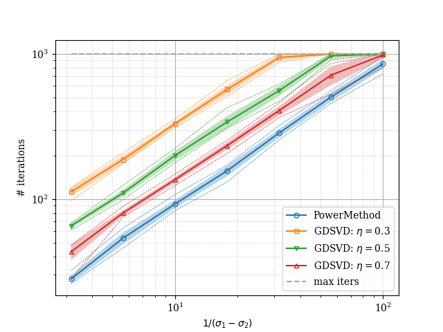
In Fig.1(a) we report the growth of the number of iterations as the gap $\sigma_{1}-\sigma_{2}$ changes running both the power method and gradient descent for finding the leading singular value and its corresponding vector. We generate matrices as described in the rank- $2$ setting for different values of $n\in\{50,75,100,200,\dots,1000\}$ . The curves are obtained by averaging over multiple curves. Indeed, we see that the the dependence on the gap does not depend on the size of the matrices which is consistent with our theoretical findings in Theorem 1.

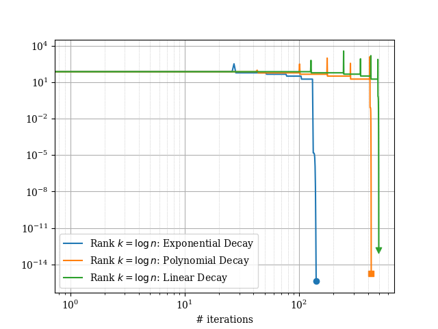
In Fig. 1(b), we illustrate the convergence of the $k$ -SVD method with gradient descent. The plots were obtained by running the method on matrices generated according to the rank- $\log(n)$ setting with $n=1000$ . The results show that indeed the method converges as suggested by the theory (see Theorem 2).

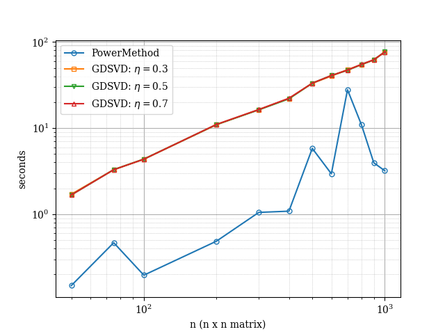
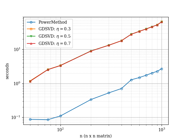
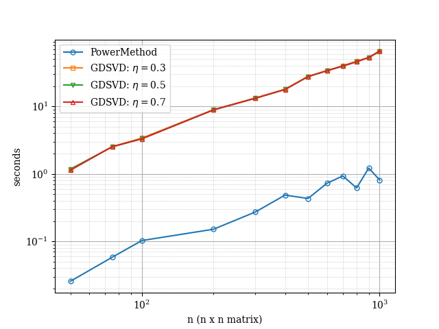
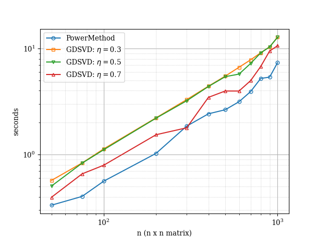
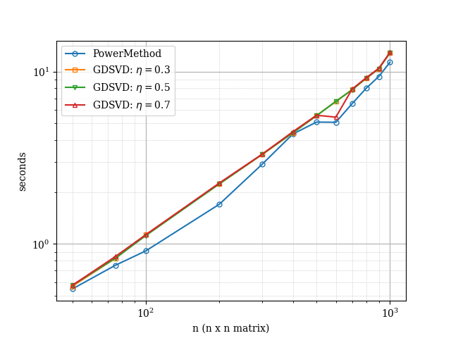
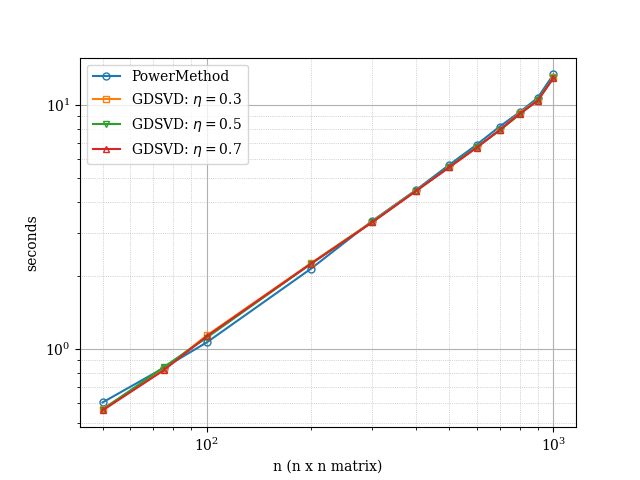
In Fig. 3 and Fig. 4 we report the evolution of the runtime of the various considered methods against the size of the matrices. Overall, we see that both, the $k$ -SVD method with gradient descent and with power method behave have similar performance. When the singular values are decaying linearly, we notice that the power method has some level of variance as the size increase suggesting some numerical instability of sorts but the methods do converge. In contrast, the $k$ -SVD method with gradient descent performs consistently across all experiments, thus suggesting robustness of the method.

6 Discussion & Conclusion

In this work, we presented a method for $k$ -SVD with gradient descent. The proposed gradient descent method uses an appealingly simple adaptive step-size towards optimizing a non-convex matrix factorization objective. We showed that the gradient method enjoys global linear convergence guarantee with random initialization in spite of the convexity of the optimization landscape. The method is shown to converge in the under parameterized setting, a result which to the best of our knowledge has eluded prior work. Critical to our convergence analysis is the observation that the gradient method behaves like Heron’s method. We believe this observation offers an interesting insight that might be of independent interest in the study of nonconvex optimization landscapes. Finally, we carried experimental results to corroborate our findings.

Because of modern computing infrastructure that allow for efficient and optimized deployment of gradient methods at scale, our method is likely to find use for computing $k$ -SVD for massively large matrices. Therefore a natural extension of our work is to develop a parallelized version of the gradient method and test it on massively large matrices.

Furthermore, gradient methods are known to possess robustness properties, thus we foresee that our proposed method will find widespread applications and further development, for settings where data is incomplete or noisy. In addition to this, a natural question is to investigate whether acceleration schemes may enhance the performance of the method, notably by reducing number of iterations required to achieve $\epsilon$ accuracy from $\log(1/\epsilon)/(\sigma_{1}-\sigma_{2})$ to $\log(1/\epsilon)/\sqrt{(\sigma_{1}-\sigma_{2})}$ . Finally, another exciting direction is extending our method to solve tensor decompositions which are known to be notoriously expansive.

References

ACLS [12] Raman Arora, Andrew Cotter, Karen Livescu, and Nathan Srebro. Stochastic optimization for pca and pls. In 2012 50th annual allerton conference on communication, control, and computing (allerton), pages 861–868. IEEE, 2012.
BH [89] Pierre Baldi and Kurt Hornik. Neural networks and principal component analysis: Learning from examples without local minima. Neural networks, 2(1):53–58, 1989.
BM [03] Samuel Burer and Renato DC Monteiro. A nonlinear programming algorithm for solving semidefinite programs via low-rank factorization. Mathematical programming, 95(2):329–357, 2003.
BNR [10] Laura Balzano, Robert Nowak, and Benjamin Recht. Online identification and tracking of subspaces from highly incomplete information. In 2010 48th Annual allerton conference on communication, control, and computing (Allerton), pages 704–711. IEEE, 2010.
CCF⁺ [21] Yuxin Chen, Yuejie Chi, Jianqing Fan, Cong Ma, et al. Spectral methods for data science: A statistical perspective. Foundations and Trends® in Machine Learning, 14(5):566–806, 2021.
CCFM [19] Yuxin Chen, Yuejie Chi, Jianqing Fan, and Cong Ma. Gradient descent with random initialization: Fast global convergence for nonconvex phase retrieval. Mathematical Programming, 176:5–37, 2019.
CLC [19] Yuejie Chi, Yue M Lu, and Yuxin Chen. Nonconvex optimization meets low-rank matrix factorization: An overview. IEEE Transactions on Signal Processing, 67(20):5239–5269, 2019.
CLS [15] Emmanuel J Candes, Xiaodong Li, and Mahdi Soltanolkotabi. Phase retrieval via wirtinger flow: Theory and algorithms. IEEE Transactions on Information Theory, 61(4):1985–2007, 2015.
CTP [19] Joshua Cape, Minh Tang, and Carey E Priebe. The two-to-infinity norm and singular subspace geometry with applications to high-dimensional statistics. 2019.
CW [02] Jane K Cullum and Ralph A Willoughby. Lanczos algorithms for large symmetric eigenvalue computations: Vol. I: Theory. SIAM, 2002.
DHL [18] Simon S Du, Wei Hu, and Jason D Lee. Algorithmic regularization in learning deep homogeneous models: Layers are automatically balanced. Advances in neural information processing systems, 31, 2018.
DK [90] James Demmel and William Kahan. Accurate singular values of bidiagonal matrices. SIAM Journal on Scientific and Statistical Computing, 11(5):873–912, 1990.
DSRO [15] Christopher De Sa, Christopher Re, and Kunle Olukotun. Global convergence of stochastic gradient descent for some non-convex matrix problems. In International conference on machine learning, pages 2332–2341. PMLR, 2015.
Fra [61] John GF Francis. The qr transformation a unitary analogue to the lr transformation—part 1. The Computer Journal, 4(3):265–271, 1961.
GH [15] Dan Garber and Elad Hazan. Fast and simple pca via convex optimization. arXiv preprint arXiv:1509.05647, 2015.
GHJ⁺ [16] Dan Garber, Elad Hazan, Chi Jin, Cameron Musco, Praneeth Netrapalli, Aaron Sidford, et al. Faster eigenvector computation via shift-and-invert preconditioning. In International Conference on Machine Learning, pages 2626–2634. PMLR, 2016.
GHJY [15] Rong Ge, Furong Huang, Chi Jin, and Yang Yuan. Escaping from saddle points—online stochastic gradient for tensor decomposition. In Conference on learning theory, pages 797–842. PMLR, 2015.
GJZ [17] Rong Ge, Chi Jin, and Yi Zheng. No spurious local minima in nonconvex low rank problems: A unified geometric analysis. In International Conference on Machine Learning, pages 1233–1242. PMLR, 2017.
GLM [16] Rong Ge, Jason D Lee, and Tengyu Ma. Matrix completion has no spurious local minimum. Advances in neural information processing systems, 29, 2016.
H⁺ [16] Elad Hazan et al. Introduction to online convex optimization. Foundations and Trends® in Optimization, 2(3-4):157–325, 2016.
HP [14] Moritz Hardt and Eric Price. The noisy power method: A meta algorithm with applications. Advances in neural information processing systems, 27, 2014.
JGN⁺ [17] Chi Jin, Rong Ge, Praneeth Netrapalli, Sham M Kakade, and Michael I Jordan. How to escape saddle points efficiently. In International conference on machine learning, pages 1724–1732. PMLR, 2017.
JJKN [17] Prateek Jain, Chi Jin, Sham Kakade, and Praneeth Netrapalli. Global convergence of non-convex gradient descent for computing matrix squareroot. In Artificial Intelligence and Statistics, pages 479–488. PMLR, 2017.
JWP⁺ [24] Xixi Jia, Hailin Wang, Jiangjun Peng, Xiangchu Feng, and Deyu Meng. Preconditioning matters: Fast global convergence of non-convex matrix factorization via scaled gradient descent. Advances in Neural Information Processing Systems, 36, 2024.
Lan [50] Cornelius Lanczos. An iteration method for the solution of the eigenvalue problem of linear differential and integral operators. 1950.
LSJR [16] Jason D Lee, Max Simchowitz, Michael I Jordan, and Benjamin Recht. Gradient descent converges to minimizers. arXiv preprint arXiv:1602.04915, 2016.
LZMH [24] Bingcong Li, Liang Zhang, Aryan Mokhtari, and Niao He. On the crucial role of initialization for matrix factorization. arXiv preprint arXiv:2410.18965, 2024.
MPG [29] RV Mises and Hilda Pollaczek-Geiringer. Praktische verfahren der gleichungsauflösung. ZAMM-Journal of Applied Mathematics and Mechanics/Zeitschrift für Angewandte Mathematik und Mechanik, 9(1):58–77, 1929.
OK [85] Erkki Oja and Juha Karhunen. On stochastic approximation of the eigenvectors and eigenvalues of the expectation of a random matrix. Journal of mathematical analysis and applications, 106(1):69–84, 1985.
Sha [15] Ohad Shamir. A stochastic pca and svd algorithm with an exponential convergence rate. In International conference on machine learning, pages 144–152. PMLR, 2015.
SMS⁺ [24] Łukasz Struski, Paweł Morkisz, Przemysław Spurek, Samuel Rodriguez Bernabeu, and Tomasz Trzciński. Efficient gpu implementation of randomized svd and its applications. Expert Systems with Applications, 248:123462, 2024.
SS [21] Dominik Stöger and Mahdi Soltanolkotabi. Small random initialization is akin to spectral learning: Optimization and generalization guarantees for overparameterized low-rank matrix reconstruction. Advances in Neural Information Processing Systems, 34:23831–23843, 2021.
Ste [93] Gilbert W Stewart. On the early history of the singular value decomposition. SIAM review, 35(4):551–566, 1993.
TMC [21] Tian Tong, Cong Ma, and Yuejie Chi. Accelerating ill-conditioned low-rank matrix estimation via scaled gradient descent. Journal of Machine Learning Research, 22(150):1–63, 2021.
XSCM [23] Xingyu Xu, Yandi Shen, Yuejie Chi, and Cong Ma. The power of preconditioning in overparameterized low-rank matrix sensing. In International Conference on Machine Learning, pages 38611–38654. PMLR, 2023.
ZFZ [23] Gavin Zhang, Salar Fattahi, and Richard Y Zhang. Preconditioned gradient descent for overparameterized nonconvex burer–monteiro factorization with global optimality certification. Journal of Machine Learning Research, 24(163):1–55, 2023.
ZJRS [16] Hongyi Zhang, Sashank J Reddi, and Suvrit Sra. Riemannian svrg: Fast stochastic optimization on riemannian manifolds. Advances in Neural Information Processing Systems, 29, 2016.

Appendix A Proofs

A.1 Proof of Proposition 1

Proof of Proposition 1.

First, we immediately see that the event $\{\|x_{1}\|\neq 0,\quad\text{and}\quad x_{1}=\|x_{1}\|u_{1}\}$ holds almost surely.

We start with the observation that for all $t\geq 1$ , $|x_{t}^{\top}u_{1}|=\|x_{t}\|$ . This is because by construction the initial point $x_{1}$ is already in the span of $M$ . Next, we have that for all $t\geq 1$ ,

\displaystyle x_{t+1}^{\top}u_{1}=\left((1-\eta)+\eta\frac{\sigma_{1}}{\|x_{t}\|^{2}}\right)x_{t}^{\top}u_{1}

which leads to

\displaystyle\|x_{t+1}\|=(1-\eta)\|x_{t}\|+\eta\frac{\sigma_{1}}{\|x_{t}\|}.

In the above we recognize the iterations of a Babylonian method (a.k.a. as Heron’s method) for finding the square root of a real number. For completeness, we provide the proof of convergence. Let us denote

\displaystyle\epsilon_{t}=\frac{\|x_{t}\|}{\sigma_{1}}-1

by replacing in the equation above we obtain that

	$\displaystyle\epsilon_{t+1}$	$\displaystyle=(1-\eta)(\epsilon_{t}+1)+\frac{\eta}{(\epsilon_{t}+1)}-1$
		$\displaystyle=\frac{(1-\eta)\varepsilon_{t}^{2}+(1-2\eta)\varepsilon_{t}}{\varepsilon_{t}+1}.$

With the choice $\eta=1/2$ , we obtain that

\displaystyle\epsilon_{t+1}=\frac{\epsilon_{t}^{2}}{2(\epsilon_{t}+1)}

from which we first conclude that for all $t\geq 1$ , $\varepsilon_{t+1}>0$ (note that we already have $\varepsilon_{t}>-1$ ). Thus we obtain

\displaystyle 0<\epsilon_{t+1}\leq\frac{1}{2}\min\left(\epsilon_{t}^{2},\epsilon_{t}\right).

This clearly implies that we have quadratic convergence. ∎

A.2 Proof of Theorem 1 and Theorem 3

Theorem 3 is an intermediate step in proving Theorem 1 and is therefore included in the proof below.

Proof of Theorem 1.

First, by applying Lemma 1 (with $\eta=1/2$ ), that after $\tau=\log(\frac{\|x_{1}\|}{\beta\sqrt{\sigma_{1}}})$ that for all $t>\tau$ , we have

\alpha\sqrt{\sigma_{1}}\leq\|x_{t}\|\leq\beta\sqrt{\sigma_{1}}.

and we also have

\displaystyle\left|\frac{\|x_{t}\|^{2}}{\sigma_{1}}-1\right|\leq\left|\frac{\|x_{t}\|}{\sqrt{\sigma_{1}}}-1\right|\left|\frac{\|x_{t}\|}{\sqrt{\sigma_{1}}}+1\right|\leq(\beta+1)\left|\frac{\|x_{t}\|}{\sqrt{\sigma_{1}}}-1\right|

(28)

Thus, using the decompositions 6 and applying Lemma 3 and 4, we obtain that

	$\displaystyle\\|x_{t+\tau}\pm\sqrt{\sigma_{1}}u_{1}\\|$	$\displaystyle\leq(\beta+1)\sqrt{\sigma_{1}}t\left(\left(1+\frac{\sigma_{1}-\sigma_{2}}{\beta^{2}\sigma_{1}+\sigma_{2}}\right)\vee\sqrt{2}\right)^{-2t}\left(\frac{\|\tan(\theta_{1,1})\|^{2}}{4\alpha\|\cos(\theta_{1,1})\|^{2}}\left(\beta+\frac{1}{\alpha}\right)^{2}+\frac{\|\tan(\theta_{1,1})\|}{\|\cos(\theta_{1,1})\|}\left(\beta+\frac{1}{\alpha}\right)\right)$
		$\displaystyle+\sqrt{2\sigma_{1}}\left(1+\frac{(\sigma_{1}-\sigma_{2})}{\beta^{2}\sigma_{1}+\sigma_{2}}\right)^{-t}\|\tan(\theta_{1,1})\|^{2}$

We denote

	$\displaystyle C_{1}$	$\displaystyle=(\beta+1)\left(\frac{\|\tan(\theta_{1,1})\|^{2}}{4\alpha\|\cos(\theta_{1,1})\|^{2}}\left(\beta+\frac{1}{\alpha}\right)^{2}+\frac{\|\tan(\theta_{1,1})\|}{\|\cos(\theta_{1,1})\|}\left(\beta+\frac{1}{\alpha}\right)\right)$
	$\displaystyle C_{2}$	$\displaystyle=\sqrt{2}\|\tan(\theta_{1,1})\|^{2}$

and write

\displaystyle\|x_{t+\tau}\pm\sqrt{\sigma_{1}}u_{1}\|

\displaystyle\leq C_{1}\sqrt{\sigma_{1}}t\left(\left(1+\frac{\sigma_{1}-\sigma_{2}}{\beta^{2}\sigma_{1}+\sigma_{2}}\right)\vee\sqrt{2}\right)^{-2t}+C_{2}\sqrt{\sigma_{1}}\left(1+\frac{(\sigma_{1}-\sigma_{2})}{\beta^{2}\sigma_{1}+\sigma_{2}}\right)^{-t}

We can verify that

	$\displaystyle t\geq 2\left(\frac{\beta^{2}\sigma_{1}+\sigma_{2}}{\sigma_{1}-\sigma_{2}}+1\right)\vee\left(\frac{\sqrt{2}}{\sqrt{2}-1}\right)\log\left(2\left(\frac{\beta^{2}\sigma_{1}+\sigma_{2}}{\sigma_{1}-\sigma_{2}}+1\right)\vee\left(\frac{\sqrt{2}}{\sqrt{2}-1}\right)\right)$		(29)
	$\displaystyle\qquad\qquad\qquad\qquad\qquad\qquad\qquad\qquad\qquad\implies t\geq\left(\frac{\beta^{2}\sigma_{1}+\sigma_{2}}{\sigma_{1}-\sigma_{2}}+1\right)\vee\left(\frac{\sqrt{2}}{\sqrt{2}-1}\right)\log(t)$		(30)
	$\displaystyle\qquad\qquad\qquad\qquad\qquad\qquad\qquad\qquad\qquad\implies t\left(\left(1+\frac{\sigma_{1}-\sigma_{2}}{\beta^{2}\sigma_{1}+\sigma_{2}}\right)\vee\sqrt{2}\right)^{-t}\leq 1$		(31)

where we use the elementary fact that if $t\geq 2a\log(2a)$ then $t\geq a\log(t)$ for any $a>0$ and $\log(1+x)\geq\frac{x}{1+x}$ for all $x>0$ . Thus, under condition (29) we obtain

\displaystyle\|x_{t+\tau}\pm\sqrt{\sigma_{1}}u_{1}\|

\displaystyle\leq C_{1}\sqrt{\sigma_{1}}\left(\left(1+\frac{\sigma_{1}-\sigma_{2}}{\beta^{2}\sigma_{1}+\sigma_{2}}\right)\vee\sqrt{2}\right)^{-t}+C_{2}\sqrt{\sigma_{1}}\left(1+\frac{(\sigma_{1}-\sigma_{2})}{\beta^{2}\sigma_{1}+\sigma_{2}}\right)^{-t},

In view of Lemma 6, the statement concerning $\|x_{t}x_{t}^{\top}-\sigma_{1}u_{1}u_{1}^{\top}\|$ follows similarly. At this stage we have shown the statement of Theorem 3.

We also see that

	$\displaystyle t\geq\left(\frac{\beta^{2}\sigma_{1}+\sigma_{2}}{\sigma_{1}-\sigma_{2}}+1\right)\vee\left(\frac{\sqrt{2}}{\sqrt{2}-1}\right)\log\left(\frac{2}{C_{1}\sqrt{\sigma_{1}}\epsilon}\right)$	$\displaystyle\implies C_{1}\sqrt{\sigma_{1}}\left(\left(1+\frac{\sigma_{1}-\sigma_{2}}{\beta^{2}\sigma_{1}+\sigma_{2}}\right)\vee\sqrt{2}\right)^{-t}\leq\frac{\epsilon}{2}$		(32)
	$\displaystyle t\geq\left(\frac{\beta^{2}\sigma_{1}+\sigma_{2}}{\sigma_{1}-\sigma_{2}}+1\right)\log\left(\frac{2}{C_{2}\sqrt{\sigma_{1}}\epsilon}\right)$	$\displaystyle\implies C_{1}\sqrt{\sigma_{1}}\left(1+\frac{\sigma_{1}-\sigma_{2}}{\beta^{2}\sigma_{1}+\sigma_{2}}\right)^{-t}\leq\frac{\epsilon}{2}$		(33)

where we used again the elementary fact $\log(1+x)\geq\frac{x}{1+x}$ . We conclude that if

\displaystyle t\geq c_{1}\left(\frac{\beta^{2}\sigma_{1}+\sigma_{2}}{\sigma_{1}-\sigma_{2}}\vee 1\right)\log\left(\frac{c_{2}}{\sigma_{1}\epsilon}\left(\frac{\beta^{2}\sigma_{1}+\sigma_{2}}{\sigma_{1}-\sigma_{2}}\vee 1\right)\right)\qquad\text{and}\qquad\tau=\log\left(\frac{\|x_{t}\|}{\beta\sqrt{\sigma_{1}}}\right)

then

\displaystyle\|x_{t}\pm\sqrt{\sigma_{1}}u_{1}\|\leq\epsilon.

∎

A.3 Error decompositions

Lemma 5.

Let $M,\tilde{M}\in\mathbb{R}^{n\times n}$ symmetric matrices. Let $\sigma_{1},\dots,\sigma_{n}$ (resp. $\tilde{\sigma}_{1},\dots,\tilde{\sigma}_{n}$ ) be the eigenvalues of $M$ (resp. $\tilde{M}$ ) in decreasing order, and $u_{1},\dots,u_{d}$ (resp. $\tilde{u}_{1},\dots,\tilde{u}_{k}$ ) be their corresponding eigenvectors. Then, for all $\ell\in[k]$ , we have

	$\displaystyle\min_{W\in\mathcal{O}^{\ell\times\ell}}\\|U_{1:\ell}-\tilde{U}_{1:\ell}W\\|$	$\displaystyle\leq\sqrt{2}\frac{\\|M-\tilde{M}\\|}{\sigma_{\ell}-\sigma_{\ell+1}}$		(34)
	$\displaystyle\|\sigma_{i}-\tilde{\sigma}_{i}\|$	$\displaystyle\leq\\|M-\widetilde{M}\\|$		(35)

where $\mathcal{O}^{\ell\times\ell}$ denotes the set of $\ell\times\ell$ orthogonal matrices, and using the convention that $\sigma_{d+1}=0$ .

Proof of 5.

The proof of the result is an immediate consequence of Davis-Kahan and the inequality $\min_{W\in\mathcal{O}^{\ell\times\ell}}\|U_{1:\ell}-\tilde{U}_{1:\ell}W\|\leq\|\sin(U_{1:\ell},\tilde{U}_{1:\ell})\|$ (e.g., see [9]). The second inequality is simply Weyl’s inequality ∎

Lemma 6 (Error decompositions).

When $\|x_{t}\|\neq 0$ , we have

	$\displaystyle\left\\|x_{t}x_{t}^{\top}-\sigma_{1}u_{1}u_{1}^{\top}\right\\|$	$\displaystyle\leq\,\sigma_{1}\left(3\left\|\frac{\\|x_{t}\\|^{2}}{\sigma_{1}}-1\right\|+\left\\|\frac{1}{\\|x_{t}\\|}x_{t}-u_{1}\right\\|\wedge\left\\|\frac{1}{\\|x_{t}\\|}x_{t}+u_{1}\right\\|\right)$
	$\displaystyle\\|x_{t}-\sqrt{\sigma_{1}}u_{1}\\|\wedge\\|x_{t}+\sqrt{\sigma_{1}}u_{1}\\|$	$\displaystyle\leq\sqrt{\sigma_{1}}\left(\left\|\frac{\\|x_{t}\\|^{2}}{\sigma_{1}}-1\right\|+\left\\|\frac{1}{\\|x_{t}\\|}x_{t}-u_{1}\right\\|\wedge\left\\|\frac{1}{\\|x_{t}\\|}x_{t}+u_{1}\right\\|\right)$

Proof of Lemma 6.

For ease of notation, we use the shorthand $\tilde{x}_{t}=\|x_{t}\|^{-1}x_{t}$ . First, we have:

	$\displaystyle\left\\|x_{t}x_{t}^{\top}-\sigma_{1}u_{1}u_{1}^{\top}\right\\|$	$\displaystyle=\left\\|(\\|x_{t}\\|^{2}-\sigma_{1})\left(\tilde{x}_{t}\tilde{x}_{t}^{\top}-u_{1}u_{1}^{\top}\right)+\sigma_{1}\left(\tilde{x}_{t}\tilde{x}_{t}^{\top}-u_{1}u_{1}^{\top}\right)+(\\|x_{t}\\|^{2}-\sigma_{1})u_{1}u_{1}^{\top}\right\\|$
		$\displaystyle\leq\|\\|x_{t}\\|^{2}-\sigma_{1}\|\left\\|\tilde{x}_{t}\tilde{x}_{t}^{\top}-u_{1}u_{1}^{\top}\right\\|+\sigma_{1}\left\\|\tilde{x}_{t}\tilde{x}_{t}^{\top}-u_{1}u_{1}^{\top}\right\\|+\|\\|x_{t}\\|^{2}-\sigma_{1}\|$
		$\displaystyle\leq\sigma_{1}\left(\left\|\frac{\\|x_{t}\\|^{2}}{\sigma_{1}}-1\right\|\left\\|\tilde{x}_{t}\tilde{x}_{t}^{\top}-u_{1}u_{1}^{\top}\right\\|+\left\\|\tilde{x}_{t}\tilde{x}_{t}^{\top}-u_{1}u_{1}^{\top}\right\\|+\left\|\frac{\\|x_{t}\\|^{2}}{\sigma_{1}}-1\right\|\right)$
		$\displaystyle\leq\sigma_{1}\left(3\left\|\frac{\\|x_{t}\\|^{2}}{\sigma_{1}}-1\right\|+\left\\|\tilde{x}_{t}\tilde{x}_{t}^{\top}-u_{1}u_{1}^{\top}\right\\|\right)$

Next, we also have

	$\displaystyle\left\\|\tilde{x}_{t}\tilde{x}_{t}^{\top}-u_{1}u_{1}^{\top}\right\\|^{2}$	$\displaystyle\leq\left\\|\tilde{x}_{t}\tilde{x}_{t}^{\top}-u_{1}u_{1}^{\top}\right\\|_{F}^{2}$
		$\displaystyle\leq(2-2(u_{1}^{\top}x_{t})^{2})$
		$\displaystyle\leq\frac{1}{2}(2-2(u_{1}^{\top}x_{t}))(2+2(u_{1}^{\top}x_{t}))$
		$\displaystyle\leq\frac{1}{2}\\|\tilde{x}_{t}-u_{1}\\|\\|\tilde{x}_{t}+u_{1}\\|$
		$\displaystyle\leq\\|\tilde{x}_{t}-u_{1}\\|\wedge\\|\tilde{x}_{t}+u_{1}\\|$

Thus we obtain

\displaystyle\left\|x_{t}x_{t}^{\top}-\sigma_{1}u_{1}u_{1}^{\top}\right\|\leq\sigma_{1}\left(3\left|\frac{\|x_{t}\|^{2}}{\sigma_{1}}-1\right|+\|\tilde{x}_{t}-u_{1}\|\wedge\|\tilde{x}_{t}+u_{1}\|\right)

(36)

Next, we have

	$\displaystyle\\|x_{t}\pm\sqrt{\sigma_{1}}u_{1}\\|$	$\displaystyle\leq\left\\|x_{t}-\frac{\sqrt{\sigma_{1}}}{\\|x_{t}\\|}x_{t}+\frac{\sqrt{\sigma_{1}}}{\\|x_{t}\\|}x_{t}\pm\sqrt{\sigma_{1}}u_{1}\right\\|$
		$\displaystyle\leq\left\\|\frac{x_{t}}{\\|x_{t}\\|}\right\\|\|\\|x_{t}\\|-\sqrt{\sigma_{1}}\|+\sqrt{\sigma_{1}}\left\\|\frac{x_{t}}{\\|x_{t}\\|}\pm u_{1}\right\\|$
		$\displaystyle\leq\sqrt{\sigma_{1}}\left\|\frac{\\|x_{t}\\|}{\sqrt{\sigma_{1}}}-1\right\|+\sqrt{\sigma_{1}}\left\\|\frac{x_{t}}{\\|x_{t}\\|}\pm u_{1}\right\\|$
		$\displaystyle\leq\sqrt{\sigma_{1}}\left\|\frac{\\|x_{t}\\|^{2}}{\sigma_{1}}-1\right\|+\sqrt{\sigma_{1}}\left\\|\frac{x_{t}}{\\|x_{t}\\|}\pm u_{1}\right\\|$

∎

A.4 Proof of Lemma 1

Proof of Lemma 1.

Our proof supposes that $x_{1}^{\top}u_{1}\neq 0$ which guaranteed almost surely by the random initialization (12).

Claim 1. First, we establish the following useful inequalities: for all $t\geq 1$ ,

$(i)$

$\|x_{t}\|>0$ .
$(ii)$

$\left((1-\eta)+\eta\frac{\sigma_{d}}{\|x_{t}\|^{2}}\right)\|x_{t}\|\leq\|x_{t+1}\|\leq\left((1-\eta)+\eta\frac{\sigma_{1}}{\|x_{t}\|^{2}}\right)\|x_{t}\|$

We start by noting that we can project the iterations of the gradient descent updates (15) onto $u_{i}$ , for all $i\in[d]$ , gives

\displaystyle u_{i}^{\top}x_{t+1}=\left((1-\eta)+\eta\frac{\sigma_{i}}{\|x_{t}\|}\right)u_{i}^{\top}x_{t}

(37)

which follows because of the simple fact that $u_{i}^{\top}M=\sigma_{i}u_{i}^{\top}$ . Thus, squaring and summing the equations (37) over $i\in[d]$ , gives

\displaystyle\|x_{t+1}\|^{2}=\sum_{i=1}^{d}\left((1-\eta)+\eta\frac{\sigma_{i}}{\|x_{t}\|^{2}}\right)^{2}|u_{i}^{\top}x_{t}|^{2}

(38)

Recalling that $\sigma_{1}\geq\cdots\geq\sigma_{d}>0$ , we immediately deduce from (38) the inequality $(ii)$ . Inequality $(i)$ because if $\|x_{1}\|>0$ , than thanks to $(ii)$ it also follows $\|x_{t}\|>0$ .

Claim 2. Let us denote for all $i\in[d]$ , $t\geq 1$ , $|\cos(\theta_{i,t})|=|u_{i}^{\top}x_{t}|/\|x_{t}|$ . We establish that the following properties hold:

$(i)$

$(|\cos(\theta_{1,t})|)_{t\geq 1}$ is non-decreasing sequence
$(ii)$

$(|\cos(\theta_{d,t})|)_{t\geq 1}$ is a non-increasing sequence
$(iii)$

for all $t\geq 1$ , $\|x_{t+1}\|\geq\alpha\sqrt{\sigma_{1}}$ .

To prove the aforementioned claim we start by noting from (37) that for all $i\in[d]$ , we have

\displaystyle\|x_{t+1}\||\cos(\theta_{i,t+1})|=\left((1-\eta)\|x_{t}\|+\eta\frac{\sigma_{i}}{\|x_{t}\|}\right)|\cos(\theta_{i,t})|

(39)

Thus, from the Claim 1 (Eq. (ii)), we immediately see that for all $t\geq 1$ , we have

	$\displaystyle 1\geq\|\cos(\theta_{1,t+1})\|$	$\displaystyle\geq\|\cos(\theta_{1,t})\|\geq\|\cos(\theta_{1,1})\|$		(40)
	$\displaystyle\|\cos(\theta_{d,t+1})\|$	$\displaystyle\leq\|\cos(\theta_{d,t})\|\leq 1,$		(41)

Now, we see that the l.h.s. inequality of Eq. (ii) in Claim 1, the combination of (40) and (39) leads to the following:

$\displaystyle\\|x_{t+1}\\|$	$\displaystyle\geq\max\left\{\left((1-\eta)\\|x_{t}\\|+\eta\frac{\sigma_{1}}{\\|x_{t}\\|}\right)\|\cos(\theta_{1,1})\|,\left((1-\eta)\\|x_{t}\\|+\eta\frac{\sigma_{d}}{\\|x_{t}\\|}\right)\right\}$	(42)
	$\displaystyle\overset{(a)}{\geq}2\sqrt{\eta(1-\eta)}\max\left\{\|\cos(\theta_{1,1})\|,\sqrt{\frac{\sigma_{d}}{\sigma_{1}}}\right\}\sqrt{\sigma_{1}}$	(43)
	$\displaystyle=\alpha\sqrt{\sigma_{1}}$	(44)

where we used in $(a)$ the elementary fact that $2\sqrt{\eta(1-\eta)\sigma}=\inf_{x>0}(1-\eta)x+\eta(\sigma/x)$ for all $\sigma>0$ . This concludes Claim 2.

Claim 3. We establish that if $\alpha\sqrt{\sigma_{1}}\leq\|x_{t}\|\leq\sqrt{\sigma_{1}}$ then, $\|x_{t+1}\|\leq\beta\sqrt{\sigma_{1}}$ .

We can immediately see from Claim 1 that

$\displaystyle\\|x_{t+1}\\|$	$\displaystyle\leq(1-\eta)\\|x_{t}\\|+\eta\frac{\sigma_{1}}{\\|x_{t}\\|}$	(45)
	$\displaystyle\leq\left((1-\eta)+\frac{\eta}{2\sqrt{\eta(1-\eta)}\max(\|\cos(\theta_{1,1})\|,\kappa^{-1/2})}\right)\sqrt{\sigma_{1}}$	(46)
	$\displaystyle\leq\left((1-\eta)+\frac{1}{2}\sqrt{\frac{\eta}{1-\eta}}\min(\|\cos(\theta_{1,1})\|^{-1},\kappa^{1/2})\right)\sqrt{\sigma_{1}}$	(47)
	$\displaystyle=\beta\sqrt{\sigma_{1}}$	(48)

where we denote $\beta=(1-\eta)+\frac{1}{2}\sqrt{\frac{\eta}{1-\eta}}\min(|\cos(\theta_{1,1})|^{-1},\sqrt{\kappa})$ and note that $\beta>1$ .

Claim 4: If $\sqrt{\sigma_{1}}<\|x_{t}\|\leq\beta\sqrt{\sigma_{1}}$ , then $\|x_{t+1}\|\leq\beta\sqrt{\sigma_{1}}$ .

Indeed, start from the inequality in Claim 1, we can immediately verify that

\displaystyle\|x_{t+1}\|\leq\left((1-\eta)+\eta\frac{\sigma_{1}}{\|x_{t}\|^{2}}\right)\|x_{t}\|\leq\|x_{t}\|\leq\beta\sqrt{\sigma_{1}}

(49)

Indeed we observe that if $\sqrt{\sigma_{1}}<\|x_{t}\|\leq\beta\sqrt{\sigma_{1}}$ , then $\sqrt{\sigma_{1}}/\|x_{t}\|\leq 1$ .

Claim 5: If $\|x_{1}\|>\beta\sqrt{\sigma_{1}}$ , then there exists $k^{\star}\geq 1$ , such that $\|x_{1+k^{\star}}\|\leq\beta\sqrt{\sigma_{1}}$ , satisfying

\displaystyle k^{\star}\leq\frac{\beta^{2}}{\eta(\beta^{2}-1)}\log\left(\frac{\|x_{t}\|}{\beta\sqrt{\sigma_{1}}}\right)

(50)

Assuming that $\|x_{t}\|>\beta\sqrt{\sigma_{1}}$ , let us define $k^{\star}=\min\{k\geq 1:\|x_{t+k}\|\leq\beta\sqrt{\sigma_{1}}\}$ , the number of iterations required for $\|x_{t+k}\|\leq\beta\sqrt{\sigma_{1}}$ . Using the r.h.s. of the inequality in Claim 1, and by definition of $k^{\star}$ , we know that for $1\leq k<k^{\star}$ ,

\displaystyle\|x_{t+k-1}\|\leq\left((1-\eta)+\eta\frac{\sigma_{1}}{\|x_{t+k}\|^{2}}\right)\|z_{t+k}\|\leq\left((1-\eta)+\eta\beta^{-2}\right)\|z_{t+k}\|.

(51)

Iterating the above inequality, we obtain that

\displaystyle\|x_{t+k^{\star}}\|\leq\left((1-\eta)+\eta\beta^{-2}\right)^{k^{\star}}\|x_{t}\|.

Now, let us note that $k^{\star}$ can not be too large. More specifically, we remark that:

\displaystyle k^{\star}\geq\frac{\eta(\beta^{2}-1)}{(1-\eta)\beta^{2}+\eta}\log\left(\frac{\|x_{t}\|}{\beta\sqrt{\sigma_{1}}}\right)\geq\frac{\log\left(\frac{\|x_{t}\|}{\beta\sigma_{1}}\right)}{\log\left(\frac{1}{(1-\eta)+\eta\beta^{-2}}\right)}\implies\left((1-\eta)+\eta\beta^{-2}\right)^{k^{\star}}\|x_{t}\|\leq\beta\sqrt{\sigma_{1}}

Therefore, it must hold that

\displaystyle k^{\star}\leq\frac{\eta(\beta^{2}-1)}{(1-\eta)\beta^{2}+\eta}\log\left(\frac{\|x_{t}\|}{\beta\sqrt{\sigma_{1}}}\right)

Note that from Claim 3 and 4, as soon as $\alpha\sqrt{\sigma_{1}}\leq\|x_{t}\|\leq\beta\sqrt{\sigma_{1}}$ , then it will never escape this region. Therefore, we only need to use Claim 5 if the first iterate $\|x_{1}\|$ is outside the region $[\alpha\sqrt{\sigma_{1}},\beta\sqrt{\sigma_{1}}]$ . ∎

A.5 Proof of Lemma 2

Proof of Lemma 2.

We prove the saddle-avoidance property of gradient descent. The proof is an immediate application of 1. Indeed, we have

	$\displaystyle\\|\nabla g(x_{t};M)\\|$	$\displaystyle=\\|\nabla Mx_{t}-\\|x_{t}\\|^{2}x_{t}\\|$
		$\displaystyle=\left\\|\sum_{i=1}^{d}(\sigma_{i}-\\|x_{t}\\|^{2})(u_{i}^{\top}x_{t})u_{i}\right\\|$
		$\displaystyle=\left(\sum_{i=1}^{d}(\sigma_{i}-\\|x_{t}\\|^{2})^{2}(u_{i}^{\top}x_{t})^{2}\right)^{1/2}$
		$\displaystyle\geq\|\sigma_{1}-\\|x_{t}\\|^{2}\|\|u_{1}^{\top}x_{t}\|$
		$\displaystyle\geq\|\sqrt{\sigma_{1}}-\\|x_{t}\\|\|\|\sqrt{\sigma_{1}}+\\|x_{t}\\|\|\\|x_{t}\\|\|\cos(\theta_{1,t})\|$
		$\displaystyle\geq\|\|\sqrt{\sigma_{1}}-\sqrt{\sigma_{i}}\|-\delta\|\sqrt{\sigma_{1}}\alpha\sqrt{\sigma_{1}}\|\cos(\theta_{1,1})\|$
		$\displaystyle\leq\alpha\sigma_{1}\|\cos(\theta_{1,1})\|\left\|\|\sqrt{\sigma_{1}}-\sqrt{\sigma_{i}}\|-\delta\right\|$

where we used Lemma 1 to bound $\|x_{t}\|\geq\alpha\sqrt{\sigma_{1}}$ and $|\cos(\theta_{i,t})|\geq|\cos(\theta_{i,1})|$ , and reverse triangular inequality ∎

A.6 Proof of Lemma 3

Proof of Lemma 3.

We start from the observation that for all $i\in[d]$ , we have

\displaystyle\|x_{t+1}\||\cos(\theta_{i,t+1})|=\left((1-\eta)\|x_{t}\|+\eta\frac{\sigma_{i}}{\|x_{t}\|}\right)|\cos(\theta_{i,t})|.

(52)

Now, note dividing the equations corresponding to $1$ and $i$ , we get

$\displaystyle\frac{\|\cos(\theta_{1,t+1})\|}{\|\cos(\theta_{i,t+1})\|}$	$\displaystyle=\frac{\left((1-\eta)\\|x_{t}\\|+\eta\frac{\sigma_{1}}{\\|x_{t}\\|}\right)}{\left((1-\eta)\\|x_{t}\\|+\eta\frac{\sigma_{i}}{\\|x_{t}\\|}\right)}\frac{\|\cos(\theta_{1,t})\|}{\|\cos(\theta_{i,t})\|}$	(53)
	$\displaystyle=\left(1+\frac{\left(\eta\frac{\sigma_{1}-\sigma_{i}}{\\|x_{t}\\|}\right)}{\left((1-\eta)\\|x_{t}\\|+\eta\frac{\sigma_{i}}{\\|x_{t}\\|}\right)}\right)\frac{\|\cos(\theta_{1,t})\|}{\|\cos(\theta_{i,t})\|}$	(54)
	$\displaystyle=\underbrace{\left(1+\frac{\eta(\sigma_{1}-\sigma_{i})}{(1-\eta)\\|x_{t}\\|^{2}+\eta\sigma_{i}}\right)}_{>1\text{ because }\sigma_{1}-\sigma_{i}>0}\frac{\|\cos(\theta_{1,t})\|}{\|\cos(\theta_{i,t})\|}$	(55)

Thus, we have for all $t\geq 1:$

\displaystyle\frac{|\cos(\theta_{i,t})|}{|\cos(\theta_{i,t+1})|}=\left(1+\frac{\eta(\sigma_{1}-\sigma_{i})}{(1-\eta)\|x_{t}\|^{2}+\eta\sigma_{i}}\right)\frac{|\cos(\theta_{1,t})|}{|\cos(\theta_{1,t+1})|},

which leads to

\displaystyle\frac{|\cos(\theta_{i,1})|}{|\cos(\theta_{i,t+1})|}=\left(\prod_{s=1}^{t}\left(1+\frac{\eta(\sigma_{1}-\sigma_{i})}{(1-\eta)\|x_{t}\|^{2}+\eta\sigma_{i}}\right)\right)\frac{|\cos(\theta_{1,1})|}{|\cos(\theta_{1,t+1})|}.

We recall that for all $t\geq t_{0}$ ,

\displaystyle|\cos(\theta_{1,t})|\leq|\cos(\theta_{1,t+1})|\leq 1\quad\text{and}\qquad\alpha\sqrt{\sigma_{1}}\leq\|x_{t}\|\leq\beta\sqrt{\sigma_{1}}

which implies that

	$\displaystyle\frac{\|\cos(\theta_{1,1})\|}{\|\cos(\theta_{1,t+1})\|}\geq\|\cos(\theta_{1,1})\|$
	$\displaystyle\left(1+\frac{\eta(\sigma_{1}-\sigma_{i})}{(1-\eta)\\|x_{t}\\|^{2}+\eta\sigma_{i}}\right)$	$\displaystyle\geq 1+\frac{\eta(\sigma_{1}-\sigma_{i})}{(1-\eta)\beta^{2}\sigma_{1}+\eta\sigma_{i}}$

Hence,

\displaystyle|\cos(\theta_{i,t+1})|\leq\left(1+\frac{\eta(\sigma_{1}-\sigma_{i})}{(1-\eta)\beta^{2}\sigma_{1}+\eta\sigma_{i}}\right)^{-t}\frac{|\cos(\theta_{i,1})|}{|\cos(\theta_{1,1})|}\underset{t\to\infty}{\longrightarrow}0.

Either $u_{1}^{\top}x_{1}>0$ or $u_{1}^{\top}x_{1}<0$ . Without loss of generality, we will present the case when $u_{1}^{\top}x_{1}>0$ , in which case $\cos(\theta_{1,1})>0$ and consequently $\cos(\theta_{1,t})>0$ . Let us further note that

	$\displaystyle\left\\|\frac{1}{\\|x_{t}\\|}x_{t}-u_{1}\right\\|^{2}$	$\displaystyle=2(1-\cos(\theta_{1,t}))$
		$\displaystyle=2\frac{1-\cos^{2}(\theta_{1,t})}{1+\cos(\theta_{1,t})}$
		$\displaystyle\leq 2\sum_{i=2}^{d}\cos^{2}(\theta_{i,t})$
		$\displaystyle\leq 2\sum_{i=2}^{d}\left(1+\frac{\eta(\sigma_{1}-\sigma_{i})}{(1-\eta)\beta^{2}\sigma_{1}+\eta\sigma_{i}}\right)^{-2t}\frac{\|\cos(\theta_{i,1})\|^{2}}{\|\cos(\theta_{1,1})\|^{2}}$
		$\displaystyle\leq 2\left(1+\frac{\eta(\sigma_{1}-\sigma_{2})}{(1-\eta)\beta^{2}\sigma_{1}+\eta\sigma_{2}}\right)^{-2t}\frac{1-\|\cos(\theta_{1,1})\|^{2}}{\|\cos(\theta_{1,1})\|^{2}}$
		$\displaystyle\leq 2\left(1+\frac{\eta(\sigma_{1}-\sigma_{2})}{(1-\eta)\beta^{2}\sigma_{1}+\eta\sigma_{2}}\right)^{-2t}\|\tan(\theta_{1,1})\|^{2}$

∎

A.7 Proof of Lemma 4

Proof of Lemma 4.

Let us denote for all $t\geq 1$

	$\displaystyle\rho_{t}$	$\displaystyle=1-\frac{\|\cos(\theta_{1,t})\|}{\|\cos(\theta_{1,t+1})\|}$		(56)
	$\displaystyle\epsilon_{t}$	$\displaystyle=\frac{\\|x_{t}\\|}{\sqrt{\sigma_{1}}}-1$		(57)

First, we verify that $\rho_{t}\underset{t\to\infty}{\longrightarrow}0$ . Indeed, we have

	$\displaystyle\rho_{t}$	$\displaystyle=1-\frac{\|\cos(\theta_{1,t})\|}{\|\cos(\theta_{1,t+1})\|}$
		$\displaystyle\leq\frac{\left\|\cos(\theta_{1,t+1})-1\right\|+\left\|1-\cos(\theta_{1,t})\right\|}{\|\cos(\theta_{1,1})\|}$
		$\displaystyle\leq\frac{1}{\|\cos(\theta_{1,1})\|}\max\left(\left\\|\frac{1}{\\|x_{t+1}\\|}x_{t+1}-u_{1}\right\\|^{2},\left\\|\frac{1}{\\|x_{t}\\|}x_{t}-u_{1}\right\\|^{2}\right)$
		$\displaystyle\leq\frac{2\|\tan(\theta_{1,1})\|}{\|\cos(\theta_{1,1})\|}\left(1+\frac{\sigma_{1}-\sigma_{2}}{\beta^{2}\sigma_{1}+\sigma_{2}}\right)^{-2t}$

where we used the fact that $(\cos(\theta_{1,t}))_{t\geq 1}$ is a non-decreasing sequence, and used Lemma 3 to obtain the final bound. Thus, we see that $\rho_{t}\underset{t\to\infty}{\longrightarrow}0$ .

Next, we also recall by assumption that $\alpha\sqrt{\sigma_{1}}\leq\|x_{1}\|\leq\beta\sqrt{\sigma_{1}}$ , and by Lemma 1 that $\alpha\sqrt{\sigma_{1}}\leq\|x_{t}\|\leq\beta\sqrt{\sigma_{1}}$ for all $t\geq 1$ . Thus, we have:

\displaystyle-1<\alpha-1\leq\epsilon_{t}\leq\beta-1

(58)

Now, let us show that $\epsilon_{t}\underset{t\to\infty}{\longrightarrow}0$ . We recall that

\displaystyle\|x_{t+1}\||\cos(\theta_{1,t+1})|=\left((1-\eta)\|x_{t}\|+\eta\frac{\sigma_{1}}{\|x_{t}\|}\right)|\cos(\theta_{1,t})|.

(59)

Thus, we have

$\displaystyle\epsilon_{t+1}$	$\displaystyle=\left((1-\eta)(\epsilon_{t}+1)+\frac{\eta}{\epsilon_{t}+1}\right)(1-\rho_{t})-1$	(60)
	$\displaystyle=\left((1-\eta)(\epsilon_{t}+1)+\frac{\eta}{\epsilon_{t}+1}\right)-1-\rho_{t}\left((1-\eta)(\epsilon_{t}+1)+\frac{\eta}{\epsilon_{t}+1}\right)$	(61)
	$\displaystyle=\frac{(1-\eta)\epsilon_{t}^{2}+(1-2\eta)\epsilon_{t}}{(\epsilon_{t}+1)}-\rho_{t}\left((1-\eta)(\epsilon_{t}+1)+\frac{\eta}{\epsilon_{t}+1}\right)$	(62)
	$\displaystyle=\frac{\epsilon_{t}^{2}}{2(\epsilon_{t}+1)}-\frac{\rho_{t}}{2}\left((\epsilon_{t}+1)+\frac{1}{\epsilon_{t}+1}\right)$	(63)

where in the last equality we used $\eta=1/2$ . We conclude from the above that for all $t\geq 1$

	$\displaystyle\varepsilon_{t+1}$	$\displaystyle\geq\max\left(-\frac{\rho_{t}}{2}\left(\beta+\frac{1}{\alpha}\right),\alpha-1\right)=-\min\left(\frac{\rho_{t}}{2}\left(\beta+\frac{1}{\alpha}\right),1-\alpha\right)$
	$\displaystyle\varepsilon_{t+1}$	$\displaystyle\leq\frac{\epsilon_{t}^{2}}{2(\epsilon_{t}+1)}-\rho_{t}$

Thus, for all $t\geq 2$ , we have

	$\displaystyle\|\varepsilon_{t+1}\|$	$\displaystyle\leq\frac{\epsilon_{t}^{2}}{2(\epsilon_{t}+1)}\mathds{1}\{\epsilon_{t}>0\}+\frac{\rho_{t}^{2}}{8\alpha}\left(\beta+\frac{1}{\alpha}\right)^{2}+\frac{\rho_{t}}{2}\left(\beta+\frac{1}{\alpha}\right)$
		$\displaystyle\leq\frac{\min(\|\epsilon_{t}\|,\|\epsilon_{t}\|^{2})}{2}+\frac{\rho_{t}^{2}}{8\alpha}\left(\beta+\frac{1}{\alpha}\right)^{2}+\frac{\rho_{t}}{2}\left(\beta+\frac{1}{\alpha}\right)$

which further gives

	$\displaystyle\|\varepsilon_{t+1}\|$	$\displaystyle\leq\sum_{k=0}^{t-2}\frac{1}{2^{k}}\left(\frac{\rho_{t-k}^{2}}{8\alpha}\left(\beta+\frac{1}{\alpha}\right)^{2}+\frac{\rho_{t-k}}{2}\left(\beta+\frac{1}{\alpha}\right)\right)$
		$\displaystyle\leq\left(\sum_{k=0}^{t-2}\frac{1}{2^{k}}\left(1+\frac{\sigma_{1}-\sigma_{2}}{\beta^{2}\sigma_{1}+\sigma_{2}}\right)^{-2t+2k}\right)\left(\frac{\|\tan(\theta_{1,1})\|^{2}}{4\alpha\|\cos(\theta_{1,1})\|^{2}}\left(\beta+\frac{1}{\alpha}\right)^{2}+\frac{\|\tan(\theta_{1,1})\|}{\|\cos(\theta_{1,1})\|}\left(\beta+\frac{1}{\alpha}\right)\right)$

To conclude, we will use the following elementary fact that for $\gamma\in(0,1)$ , we have

	$\displaystyle\sum_{k=0}^{t-2}\frac{\gamma^{t-k}}{2^{k}}$	$\displaystyle=\mathds{1}\{\gamma=1/2\}(t-1)\gamma^{t}+\mathds{1}\{\gamma\neq 1/2\}\gamma^{t}\frac{1-\frac{1}{(2\gamma)^{t-1}}}{1-\frac{1}{2\gamma}}$
		$\displaystyle\leq\mathds{1}\{\gamma=1/2\}(t-1)\gamma^{t}+\mathds{1}\{\gamma\neq 1/2\}\frac{2\gamma^{2}}{\|2\gamma-1\|}\left\|\gamma^{t-1}-\frac{1}{2^{t-1}}\right\|$
		$\displaystyle\leq\mathds{1}\{\gamma=1/2\}\frac{(t-1)}{2^{t}}+\mathds{1}\{\gamma\neq 1/2\}\gamma^{2}(t-1)\left(\frac{1}{2}\vee\gamma\right)^{t-2}$
		$\displaystyle\leq(t-1)\left(\gamma\vee\frac{1}{2}\right)^{t}$

where in our case we have

\displaystyle\gamma=\left(1+\frac{\sigma_{1}-\sigma_{2}}{\beta^{2}\sigma_{1}+\sigma_{2}}\right)^{-2}=\left(\frac{\beta^{2}\sigma_{1}+\sigma_{2}}{(\beta^{2}+1)\sigma_{1}}\right)^{2}

Indeed, we obtain that

\displaystyle|\epsilon_{t+1}|\leq\left(t-1\right)\left(\left(1+\frac{\sigma_{1}-\sigma_{2}}{\beta^{2}\sigma_{1}+\sigma_{2}}\right)\vee\sqrt{2}\right)^{-2t}\left(\frac{|\tan(\theta_{1,1})|^{2}}{4\alpha|\cos(\theta_{1,1})|^{2}}\left(\beta+\frac{1}{\alpha}\right)^{2}+\frac{|\tan(\theta_{1,1})|}{|\cos(\theta_{1,1})|}\left(\beta+\frac{1}{\alpha}\right)\right)

∎

A.8 Proof of Theorem 2

Proof.

We recall that $\tilde{M}_{\ell+1}=M-\sum_{i=1}^{\ell}\hat{\sigma}_{i}\hat{u}_{i}\hat{u}_{i}^{\top}$ and denote $M_{\ell+1}=M-\sum_{i=1}^{\ell}\sigma_{i}u_{i}u_{i}^{\top}$ with $M_{1}=\tilde{M}_{1}=M$ . We will also denote the leading eigenvalue of $\tilde{M}_{\ell}$ by $\tilde{\sigma}_{\ell}$ and its corresponding eigenvector by $\tilde{u}_{\ell}$ . Note that the leading singular value of $M_{\ell}$ is $\sigma_{\ell}$ and its corresponding vector is $u_{\ell}$ . We also note that

	$\displaystyle\left\\|\tilde{M}_{\ell+1}-\left(M-\sum_{i=1}^{\ell}\sigma_{i}u_{i}u_{i}^{\top}\right)\right\\|$	$\displaystyle\leq\sum_{i=1}^{\ell}\left\\|\hat{\sigma}_{i}\hat{u}_{i}\hat{u}_{i}^{\top}-\sigma_{i}u_{i}u_{i}^{\top}\right\\|$		(64)
		$\displaystyle\leq\sum_{i=1}^{\ell}\left\\|\hat{\sigma}_{i}\hat{u}_{i}\hat{u}_{i}^{\top}-\tilde{\sigma}_{i}\tilde{u}_{i}\tilde{u}_{i}^{\top}\right\\|+\left\\|\tilde{\sigma}_{i}\tilde{u}_{i}\tilde{u}_{i}^{\top}-\sigma_{i}u_{i}u_{i}^{\top}\right\\|$		(65)

By application of gradient descent (2), we know that if method is run for $t$ large enough then for all for each $i\in[k]$ , we have the guarantee:

$\displaystyle\|\tilde{\sigma}_{i}-\hat{\sigma}_{i}\|$	$\displaystyle\leq\epsilon$	(67)
$\displaystyle\\|\hat{u}_{i}+\tilde{u}_{1}\\|\wedge\\|\hat{u}_{i}-\tilde{u}_{i}\\|$	$\displaystyle\leq\epsilon$	(68)
$\displaystyle\\|\tilde{\sigma}_{i}\tilde{u}_{i}\tilde{u}_{1}^{\top}-\hat{\sigma}_{i}\hat{u}_{i}\hat{u}_{i}^{\top}\\|$	$\displaystyle\leq\epsilon$	(69)

Now, we show by induction that things remain well behaved. (for $\ell=1$ ), we have

	$\displaystyle\|\tilde{\sigma}_{1}-\sigma_{1}\|$	$\displaystyle=0$
	$\displaystyle\|u_{1}-\tilde{u}_{1}\|$	$\displaystyle=0$
	$\displaystyle\|\sigma_{1}u_{1}u_{1}^{\top}-\sigma_{1}\tilde{u}_{1}\tilde{u}_{1}$	$\displaystyle=0$

(for $\ell=2$ ) We have

$\displaystyle\|\tilde{\sigma}_{2}-\sigma_{2}\|$	$\displaystyle\leq\epsilon$		(70)
$\displaystyle\\|\hat{u}_{2}+\tilde{u}_{2}\\|\wedge\\|\hat{u}_{2}-\tilde{u}_{2}\\|$	$\displaystyle\leq\frac{\sqrt{2}\epsilon}{\sigma_{2}-\sigma_{3}}$	$\displaystyle(\text{Lemma \ref{lem:spectral-perturbation}})$	(71)
$\displaystyle\\|\tilde{\sigma}_{2}\tilde{u}_{2}\tilde{u}_{1}^{\top}-\hat{\sigma}_{2}\hat{u}_{2}\hat{u}_{2}^{\top}\\|$	$\displaystyle\leq 3\epsilon+\frac{\sigma_{2}\sqrt{2}\epsilon}{\sigma_{2}-\sigma_{3}}$	$\displaystyle(\text{Lemma \ref{lem:error-decomposition}})$	(72)

(for $\ell=3$ ) we have

$\displaystyle\|\tilde{\sigma}_{3}-\sigma_{3}\|$	$\displaystyle\leq\epsilon+\left(\epsilon+3\epsilon+\frac{\sigma_{2}\sqrt{2}\epsilon}{\sigma_{2}-\sigma_{3}}\right)=\left(5+\frac{\sigma_{2}\sqrt{2}}{\sigma_{2}-\sigma_{3}}\right)\epsilon$		(73)
$\displaystyle\\|\hat{u}_{3}+\tilde{u}_{3}\\|\wedge\\|\hat{u}_{3}-\tilde{u}_{3}\\|$	$\displaystyle\leq\frac{\sqrt{2}}{\sigma_{3}-\sigma_{4}}\left(5+\frac{\sigma_{2}\sqrt{2}}{\sigma_{2}-\sigma_{3}}\right)\epsilon$	$\displaystyle(\text{Lemma \ref{lem:spectral-perturbation}})$	(74)
$\displaystyle\\|\tilde{\sigma}_{3}\tilde{u}_{3}\tilde{u}_{3}^{\top}-\hat{\sigma}_{3}\hat{u}_{3}\hat{u}_{3}^{\top}\\|$	$\displaystyle\leq\left(3\left(5+\frac{\sigma_{2}\sqrt{2}}{\sigma_{2}-\sigma_{3}}\right)+\frac{\sqrt{2}\sigma_{3}}{\sigma_{3}-\sigma_{4}}\left(5+\frac{\sigma_{2}\sqrt{2}}{\sigma_{2}-\sigma_{3}}\right)\right)\epsilon$	$\displaystyle(\text{Lemma \ref{lem:error-decomposition}})$	(75)

and so forth, we see that at the end the error is at most

$\displaystyle\|\tilde{\sigma}_{\ell}-\sigma_{\ell}\|$	$\displaystyle\leq kC_{3}^{k}\left(\max_{i\in[k]}\left(\frac{\sigma_{i}}{\sigma_{i}-\sigma_{i+1}}\right)\vee 1\right)^{k-1}\epsilon$	(76)
$\displaystyle\\|\hat{u}_{\ell}+\tilde{u}_{\ell}\\|\wedge\\|\hat{u}_{\ell}-\tilde{u}_{\ell}\\|$	$\displaystyle\leq kC^{k}\frac{1}{\sigma_{\ell}}\left(\max_{i\in[k]}\left(\frac{\sigma_{i}}{\sigma_{i}-\sigma_{i+1}}\right)\vee 1\right)^{k-1}\epsilon$	(77)
$\displaystyle\\|\tilde{\sigma}_{\ell}\tilde{u}_{\ell}\tilde{u}_{\ell}^{\top}-\hat{\sigma}_{\ell}\hat{u}_{\ell}\hat{u}_{\ell}^{\top}\\|$	$\displaystyle\leq kC^{k}\left(\max_{i\in[k]}\left(\frac{\sigma_{i}}{\sigma_{i}-\sigma_{i+1}}\right)\vee 1\right)^{k-1}\epsilon$	(78)

Let us denote

\displaystyle kC^{k}\left(\max_{i\in[k]}\left(\frac{\sigma_{i}}{\sigma_{i}-\sigma_{i+1}}\right)\vee 1\right)^{k-1}\epsilon=\frac{\epsilon^{\prime}}{2}.

(79)

If $\epsilon^{\prime}$ is such that $\sigma_{i}-\sigma_{i+1}>2k\epsilon^{\prime}$ , for $i\in[d]$ , and $\sigma_{n}\geq 2k\epsilon^{\prime}$ , then it will be ensured that the singular values of $\tilde{M}_{\ell}$ remain close to those of $M_{\ell}$ and $\tilde{M}_{\ell}$ stays positive definite. We may then apply gradient descent and use Theorem 1. Now, for a given $\epsilon^{\prime}$ , and a precision $\epsilon$ satisfying (79), by Theorem 1, running gradient descent long enough, namely $t_{\circ}$ , ensures that:

	$\displaystyle\|\tilde{\sigma}_{i}-\sigma_{i}\|$	$\displaystyle\leq\epsilon^{\prime}$
	$\displaystyle\sigma_{i}(\\|u_{i}+\hat{u}_{i}\\|\wedge\\|u_{i}-\hat{u}_{i}\\|)$	$\displaystyle\leq\epsilon^{\prime}$
	$\displaystyle\\|\sigma_{i}u_{i}u_{1}^{\top}-\hat{\sigma}_{i}\hat{u}_{i}\hat{u}_{i}\\|$	$\displaystyle\leq\epsilon^{\prime}$
	$\displaystyle\\|\sqrt{\sigma_{i}}u_{i}-\sqrt{\hat{\sigma}_{i}}\hat{u}_{i}\hat{u}_{i}\\|\wedge\\|\sqrt{\sigma_{i}}u_{i}+\sqrt{\hat{\sigma}_{i}}\hat{u}_{i}\hat{u}_{i}\\|$	$\displaystyle\leq\epsilon^{\prime}$

More precisely, $t_{\circ}$ is given by

\displaystyle t_{\circ}\geq C_{1}\max_{i\in[k]}\left(\frac{\sigma_{i}}{\sigma_{i}-\sigma_{i+1}}\vee 1\right)\left(k\log\left(C_{2}\max_{i\in[k]}\left(\frac{\sigma_{i}}{\sigma_{i}-\sigma_{i}}\vee 1\right)\right)+\log\left(\frac{k}{\epsilon^{\prime}}\right)\right)

In total, we need the total number of iterations to be

\displaystyle t\geq C_{1}k\max_{i\in[k]}\left(\frac{\sigma_{i}}{\sigma_{i}-\sigma_{i+1}}\vee 1\right)\left(k\log\left(C_{2}\max_{i\in[k]}\left(\frac{\sigma_{i}}{\sigma_{i}-\sigma_{i}}\vee 1\right)\right)+\log\left(\frac{k}{\epsilon^{\prime}}\right)\right)

∎

A.9 Properties of the nonconvex objective $g$

In the following lemma, we present a characterization of the properties of critical points of $g$ :

Lemma 7 (1 ${}^{\textrm{st}}$ and 2 ${}^{\textrm{nd}}$ order optimality conditions).

Let $x\in\mathbb{R}^{n}$ , the following properties hold:

(i)

$x$ is a critical point, i.e. $\nabla g(x;M)=0$ , if and only if $x=0$ or $x=\pm\sqrt{\sigma_{i}}u_{i}$ , $i\in[k]$ .
(ii)

if for all $i\neq 1$ , $\sigma_{1}>\sigma_{i}$ , then all local minima of the loss function $g$ are also global minima²²2We recall that $x$ is a local minima of $g$ iff $\nabla g(x)=0$ and $\lambda_{\min}(\nabla^{2}g(x))\geq 0$ ., and all other critical points are strict saddle³³3We recall that $x$ is a strict saddle point iff $\nabla g(x)=0$ , and $\lambda_{\min}(\nabla^{2}g(x))<0$ .. More specifically, the only local and global minima of $g$ are the points $-\sqrt{\sigma_{1}}u_{1}$ and $+\sqrt{\sigma_{1}}u_{1}$ .

A proof of Lemma 7 can be found for instance in [7].

Appendix B Implementation and Experiments

In this section, we present and validate a GPU-friendly implementation of the $k$ -SVD methods discussed in §5. This implementation was developed on 6-core, 12-thread Intel chip, and tested on a 10-core, 20-thread Intel chip and NVIDIA CUDA 12.7.

B.1 Implementation details

Notation.

We use $U_{\ell}$ to denote the $\ell^{th}$ singular vector (column) of $U$ , $V^{\top}_{\ell}$ to denote the $\ell^{th}$ singular vector (row) of $V^{\top}$ , and $S_{\ell}$ to denote the $\ell^{th}$ entry.

Algorithm 1 Computes rank-SVD of an

m\times n

matrix

M

via power method

U\leftarrow

a random

n\times k

semi-orthogonal matrix

V\leftarrow

a random

n\times k

semi-orthogonal matrix

S\leftarrow\vec{1}_{k}

M_{1}\leftarrow M

for

\ell=1,...,k

while

t<T

and (

\|U_{\ell,t+1}-U_{\ell,t}\|_{2}\geq\epsilon

\|V^{\top}_{\ell,t+1}-V^{\top}_{\ell,t}\|_{2}\geq\epsilon

) do

U_{\ell}\leftarrow M_{\ell}V^{\top}_{\ell}

V^{\top}_{\ell}\leftarrow M_{\ell}^{\top}U_{\ell}

S_{\ell}\leftarrow\|U_{\ell}\|_{2}\|V^{\top}_{\ell}\|_{2}

U_{\ell}\leftarrow U_{\ell}/\|U_{\ell}\|_{2}

V^{\top}_{\ell}\leftarrow V^{\top}_{\ell}/\|V^{\top}_{\ell}\|_{2}

t\leftarrow t+1

M_{\ell+1}\leftarrow M_{\ell}-S_{\ell}U_{\ell}V^{\top}_{\ell}

Return

U,S,V^{\top}

Algorithm 2 Computes

k

-SVD of an

m\times n

matrix

M

via gradient descent with step size

\eta/\|x\|^{2}

U\leftarrow

a random

n\times k

semi-orthogonal matrix

V\leftarrow

a random

n\times k

semi-orthogonal matrix

S\leftarrow\vec{1}_{k}

M_{\ell}\leftarrow M

for

\ell=1,...,k

x_{1}\leftarrow M_{\ell}V^{\top}_{\ell}

while

t<T

and

\left\|\frac{x_{t+1}}{\|x_{t+1}\|_{2}}-\frac{M_{\ell}M_{\ell}^{\top}x_{t}}{\|x_{t}\|_{2}^{2}}\right\|_{2}\geq\epsilon

S_{\ell}\leftarrow\|x_{t}\|_{2}

U_{\ell}\leftarrow x_{t}/\|x_{t}\|_{2}

V^{\top}_{\ell}\leftarrow M_{\ell}^{\top}x_{t}/\|x_{t}\|

x_{t+1}\leftarrow(1-\eta)x_{t}+\frac{\eta}{\|x_{t}\|^{2}}M_{\ell}M_{\ell}^{\top}x_{t}

t\leftarrow t+1

M_{\ell}\leftarrow M_{\ell}-S_{\ell}U_{\ell}V^{\top}_{\ell}

Return

U,S,V^{\top}

Notes on implementation. A temporary file to store $M_{\ell}$ is memory-mapped during computation, rather than subtracting off previous rank-approximations each time $M_{\ell}$ is required. The latter takes only $O(1)$ memory but significantly slows computation. The centralized implementations were written in Python 3.x and these are the versions tested for correctness guarantees. All of the tested SVD methods spend the most time on matrix-vector multiplication, which is easily parallelizable by spawning threads each responsible for computing one index of the resulting vector, so that each thread only requires $O(\max\{n,m\})$ space and time. Several implementations of parallelization were tested:

•

Cython: native Python fed through Cython
•

Numba: functions are jitted with Numba decorators
•

CuPy: $U,S,V^{\top}$ and temporary variables are instantiated on the GPU device, rows/columns of $M$ are moved to the device when used for computation
•

C/OpenCilk: a C implementation was attempted with parallel library OpenCilk but it suffered from numerical stability issues and required a great deal of step-size engineering

None were satisfactory in reducing the scaling of runtime with input matrix size, possibly due to unideal memory management, but CUDA specific programming may be able to improve performance.

B.2 Correctness testing

Synthetic datasets with various singular value profiles were generated to test correctness. All datasets consist of $M,U,S,V^{\top}$ stored in binary files, where $U,S,V^{\top}$ are generated according to a scheme detailed below and $M$ computed as the $n\times n$ square matrix result of $USV^{\top}$ ( $n$ ranges from 50 to 1,000).

Synthetic $U,S,V^{\top}$ schemes.

1.
Rank $\log n$ dataset. $U$ is a $n\times\lfloor\log n\rfloor$ orthonormal matrix generated using scipy.stats.ortho_group and $V^{\top}$ a $\lfloor\log n\rfloor\times n$ matrix generated the same way and transposed.
- •
  
  Exponential decay: $\sigma_{i}=a^{-i}$ where $a$ is generated by numpy.random.randint(1,10)
- •
  
  Polynomial decay: $\sigma_{i}=1/({i+1})$
- •
  
  Linear decay: $\sigma_{i}=a-bi$ , where $a$ is generated by numpy.random.randint(1,10) and $b$ is generated by numpy.random.rand(), regenerating until $\sigma_{i}>0\quad\forall i$
2.

Rank 2 dataset. $U$ is a $n\times 2$ orthonormal matrix generated using scipy.stats.ortho_group and $V^{\top}$ a $2\times n$ matrix generated the same way and transposed. $\sigma_{1}=1$ and $\sigma_{2}$ chosen as $\sigma_{1}-10^{-\delta}$ for $\delta\in[0.25,5]$ in $0.25$ increments.

Test procedure.

Test files were memory-mapped using np.memmap and checked for contiguous formatting using np.contiguousarray before passing into any SVD method. We record several metrics:

•

Approximation error: $\|M-USV^{\top}\|_{F}$
•

Subspace error: $\|U^{\top}U-\hat{U}^{\top}\hat{U}\|_{F}$ (analogous for $V^{\top}$ )
•

Orthogonal error: $\|UU^{\top}-I_{n}\|_{F}$ (analogous for $V^{\top}$ )

including partial errors at the end of each iteration, as well as total runtime and final errors.

	$\displaystyle\left\\|\frac{x_{t}}{\\|x_{t}\\|}-u_{1}\right\\|\wedge\left\\|\frac{x_{t}}{\\|x_{t}\\|}+u_{1}\right\\|$	$\displaystyle\leq\frac{\sqrt{2}}{(1+\Delta_{2})^{t-\tau}}\left\|\tan(\theta_{1,1})\right\|,$
	$\displaystyle\|\cos(\theta_{i,t+1})\|$	$\displaystyle\leq\frac{1}{(1+\Delta_{i})^{t-\tau}}\frac{\|\cos(\theta_{i,1})\|}{\|\cos(\theta_{1,1})\|},$

	$\displaystyle\min_{W\in\mathcal{O}^{\ell\times\ell}}\\|U_{1:\ell}-\tilde{U}_{1:\ell}W\\|$	$\displaystyle\leq\sqrt{2}\frac{\\|M-\tilde{M}\\|}{\sigma_{\ell}-\sigma_{\ell+1}}$		(34)
	$\displaystyle\|\sigma_{i}-\tilde{\sigma}_{i}\|$	$\displaystyle\leq\\|M-\widetilde{M}\\|$		(35)

	$\displaystyle\left\\|x_{t}x_{t}^{\top}-\sigma_{1}u_{1}u_{1}^{\top}\right\\|$	$\displaystyle\leq\,\sigma_{1}\left(3\left\|\frac{\\|x_{t}\\|^{2}}{\sigma_{1}}-1\right\|+\left\\|\frac{1}{\\|x_{t}\\|}x_{t}-u_{1}\right\\|\wedge\left\\|\frac{1}{\\|x_{t}\\|}x_{t}+u_{1}\right\\|\right)$
	$\displaystyle\\|x_{t}-\sqrt{\sigma_{1}}u_{1}\\|\wedge\\|x_{t}+\sqrt{\sigma_{1}}u_{1}\\|$	$\displaystyle\leq\sqrt{\sigma_{1}}\left(\left\|\frac{\\|x_{t}\\|^{2}}{\sigma_{1}}-1\right\|+\left\\|\frac{1}{\\|x_{t}\\|}x_{t}-u_{1}\right\\|\wedge\left\\|\frac{1}{\\|x_{t}\\|}x_{t}+u_{1}\right\\|\right)$

	$\displaystyle\left\\|x_{t}x_{t}^{\top}-\sigma_{1}u_{1}u_{1}^{\top}\right\\|$	$\displaystyle=\left\\|(\\|x_{t}\\|^{2}-\sigma_{1})\left(\tilde{x}_{t}\tilde{x}_{t}^{\top}-u_{1}u_{1}^{\top}\right)+\sigma_{1}\left(\tilde{x}_{t}\tilde{x}_{t}^{\top}-u_{1}u_{1}^{\top}\right)+(\\|x_{t}\\|^{2}-\sigma_{1})u_{1}u_{1}^{\top}\right\\|$
		$\displaystyle\leq\|\\|x_{t}\\|^{2}-\sigma_{1}\|\left\\|\tilde{x}_{t}\tilde{x}_{t}^{\top}-u_{1}u_{1}^{\top}\right\\|+\sigma_{1}\left\\|\tilde{x}_{t}\tilde{x}_{t}^{\top}-u_{1}u_{1}^{\top}\right\\|+\|\\|x_{t}\\|^{2}-\sigma_{1}\|$
		$\displaystyle\leq\sigma_{1}\left(\left\|\frac{\\|x_{t}\\|^{2}}{\sigma_{1}}-1\right\|\left\\|\tilde{x}_{t}\tilde{x}_{t}^{\top}-u_{1}u_{1}^{\top}\right\\|+\left\\|\tilde{x}_{t}\tilde{x}_{t}^{\top}-u_{1}u_{1}^{\top}\right\\|+\left\|\frac{\\|x_{t}\\|^{2}}{\sigma_{1}}-1\right\|\right)$
		$\displaystyle\leq\sigma_{1}\left(3\left\|\frac{\\|x_{t}\\|^{2}}{\sigma_{1}}-1\right\|+\left\\|\tilde{x}_{t}\tilde{x}_{t}^{\top}-u_{1}u_{1}^{\top}\right\\|\right)$

	$\displaystyle\left\\|\tilde{x}_{t}\tilde{x}_{t}^{\top}-u_{1}u_{1}^{\top}\right\\|^{2}$	$\displaystyle\leq\left\\|\tilde{x}_{t}\tilde{x}_{t}^{\top}-u_{1}u_{1}^{\top}\right\\|_{F}^{2}$
		$\displaystyle\leq(2-2(u_{1}^{\top}x_{t})^{2})$
		$\displaystyle\leq\frac{1}{2}(2-2(u_{1}^{\top}x_{t}))(2+2(u_{1}^{\top}x_{t}))$
		$\displaystyle\leq\frac{1}{2}\\|\tilde{x}_{t}-u_{1}\\|\\|\tilde{x}_{t}+u_{1}\\|$
		$\displaystyle\leq\\|\tilde{x}_{t}-u_{1}\\|\wedge\\|\tilde{x}_{t}+u_{1}\\|$

kk-SVD with Gradient Descent

Abstract

1 Introduction

Theorem 1.

Theorem 2.

2 Related Work

Methods from linear algebra.

Gradient descent for nonconvex landscapes.

Nonconvex matrix factorization.

Why study the under-parameterized setting?

3 Warm-up analysis; gradient descent as Heron’s method in disguise

Proposition 1.

4 Convergence analysis: gradient descent as Heron’s method in disguise

4.1 Region of attraction

Lemma 1 (Attracting region of gradient descent).

Lemma 2 (Saddle-point avoidance).

4.2 Alignment at linear rate

Lemma 3.

4.3 Convergence with approximate Heron’s iterations

Lemma 4.

Proof sketch of Lemma 4.

4.4 Putting everything together

Theorem 3.

5 Experiments

5.1 Experimental setup

The rank-22 setting.

The rank-log⁡(n)\log(n) settings.

5.2 Implemented methods

kk-SVD with gradient descent.

kk-SVD with power method.

5.3 Results

6 Discussion & Conclusion

References

Appendix A Proofs

A.1 Proof of Proposition 1

Proof of Proposition 1.

A.2 Proof of Theorem 1 and Theorem 3

Proof of Theorem 1.

A.3 Error decompositions

Lemma 5.

Proof of 5.

Lemma 6 (Error decompositions).

Proof of Lemma 6.

A.4 Proof of Lemma 1

Proof of Lemma 1.

A.5 Proof of Lemma 2

Proof of Lemma 2.

A.6 Proof of Lemma 3

Proof of Lemma 3.

A.7 Proof of Lemma 4

Proof of Lemma 4.

A.8 Proof of Theorem 2

Proof.

A.9 Properties of the nonconvex objective gg

Lemma 7 (1st{}^{\textrm{st}} and 2nd{}^{\textrm{nd}} order optimality conditions).

Appendix B Implementation and Experiments

B.1 Implementation details

Notation.

B.2 Correctness testing

Synthetic U,S,V⊤U,S,V^{\top} schemes.

Test procedure.

$k$ -SVD with Gradient Descent

The rank- $2$ setting.

The rank- $\log(n)$ settings.

$k$ -SVD with gradient descent.

$k$ -SVD with power method.

A.9 Properties of the nonconvex objective $g$

Lemma 7 (1 ${}^{\textrm{st}}$ and 2 ${}^{\textrm{nd}}$ order optimality conditions).

Synthetic $U,S,V^{\top}$ schemes.