KMT-2017-BLG-2820 and the Nature of the Free-Floating Planet Population
Abstract
We report a new free-floating planet (FFP) candidate, KMT-2017-BLG-2820, with Einstein radius , lens-source relative proper motion , and Einstein timescale hr. It is the third FFP candidate found in an ongoing study of giant-source finite-source point-lens (FSPL) events in the KMTNet data base, and the sixth FSPL FFP candidate overall. We find no significant evidence for a host. Based on their timescale distributions and detection rates, we argue that five of these six FSPL FFP candidates are drawn from the same population as the six point-source point-lens (PSPL) FFP candidates found by Mróz et al. (2017) in the OGLE-IV data base. The distribution of the FSPL FFPs implies that they are either sub-Jovian planets in the bulge or super-Earths in the disk. However, the apparent “Einstein Desert” () would argue for the latter. Whether each of the 12 (6 FSPL and 6 PSPL) FFP candidates is truly an FFP, or simply a very wide-separation planet, can be determined at first adaptive optics (AO) light on 30m telescopes, and earlier for some. If the latter, a second epoch of AO observations could measure the projected planet-host separation with a precision . At the present time, the balance of evidence favors the unbound-planet hypothesis.
1 Introduction
Formally, free-floating planets (FFPs) are planetary mass () objects that are not bound to any star. However, from a theoretical viewpoint, one would like to distinguish between objects that formed in situ, as stars do via gravitational collapse, and those that formed in protoplanetary disks, like planets, and were subsequently ejected. This can only be done statistically, and only by a method that is sensitive to a broad range of masses that extends well below , i.e., objects that are non-luminous given current technology. That is, gravitational microlensing is the only current technique by which such studies can be carried out.
Because it is increasingly difficult to form low-mass objects by gravitational collapse, and also increasingly difficult to form high-mass objects in protoplanetary disks (and even more difficult to then eject them), one expects a “gap” (more accurately, a strong minimum) between these two regimes, which is analogous to the so-called “brown dwarf desert”. The appearance of such a “gap” would allow one to individually identify the objects that likely formed within the protoplanetary disk, thus enabling further study.
In fact, the short-timescale, single-lens/single-source (1L1S) events that are the expected signature of FFPs can also be generated by planets in wide orbits. For example, if a doppelganger of our own solar system were oriented face-on and lay half way to the Galactic center, then its “Neptune” would lie about 7.5 Einstein radii from its “Sun”. Hence, for most trajectories of the lens system relative to a background source, a microlensing event due to the “Neptune” would be indistinguishable from 1L1S, even though the planet is bound. Therefore, to distinguish between wide-orbit planets (which are themselves quite interesting) and FFPs, one must wait for the source and lens to be sufficiently displaced that they can be separately imaged. Because a putative host might be very faint, while sources range from upper main-sequence stars to giants, this means waiting until the separation is adequate to resolve at severe to extreme contrast ratios. We adopt a range of 1.2 – 1.5 FWHM from main-sequence to giant sources. With diffraction limited imaging, this requires waiting
| (1) |
where is the wavelength of the observations, is the diameter of the mirror, is the lens-source relative proper motion, and 1.25 = 1.5/1.2. For most FFP candidates discovered to date, and also for those that will be discovered in data from the next few years, this means waiting until the end of this decade, when the separations become accessible to current telescopes and when adaptive optics (AO) imaging on 30m class telescopes becomes available (thereby reducing the pre-factor in Equation (1) by a factor ).
Thus, the study of FFPs is intrinsically a long-term project.
The first approach to the study of FFPs was based on the distribution of Einstein timescales,
| (2) |
of 1L1S events. Here, is the Einstein radius and is the lens-source relative parallax. Sumi et al. (2011) found a strong excess of day events, which they interpreted as due to a population of roughly Jupiter-mass planets, with about twice the frequency of stars. However, using an independent and superior data set, Mróz et al. (2017) ruled out such an excess. Nevertheless, Mróz et al. (2017) found an excess of few-hour events, which they suggested is consistent with a population of Earth- or super-Earth-mass objects.
Of particular note in the present context, the Mróz et al. (2017) excess was separated from the main distribution by a clear gap111The gap appears despite the fact that the timescale errors are fairly large, with typical confidence intervals spanning a factor of two in , whereas the Sumi et al. (2011) excess was not. This difference is not due to the different qualities of the two data sets, but is simply the result of the respective ratios of the mean timescale of the putative planets to that of the bulge lenses from the bottom of the stellar and brown dwarf population (say ), i.e., days. For the putative Sumi et al. (2011) planets, this ratio was about 0.4. Hence, the short-timescale tail of the brown-dwarf (BD) distribution strongly overlaps the peak of the FFP distribution due to the wide range of values of and entering Equation (2). However, the corresponding ratio for the Mróz et al. (2017) excess is only about 0.08, implying that the BD-tail is negligibly small.
Given that the Jupiter FFP population is at least 8 times smaller than suggested by Sumi et al. (2011), it can hardly be studied at all using the global distribution. That is, the Jupiter FFP events result in a small excess of day events, relative to the higher-mass “background”, which is difficult to detect even statistically. Moreover, such a small excess could in principle be due to imperfect modeling of the BD population, or even to the long-timescale tail of lower-mass FFPs. By contrast, there is essentially no “background” of unrelated microlensing events for the few-hour events found by Mróz et al. (2017): the only real issues are whether these brief “bumps” in the light curve are really due to microlensing, and if so, whether these “isolated” low-mass objects are due to FFPs rather than wide-separation bound planets. Regarding the first question, Mróz et al. (2017) argued that these events are likely due to microlensing.
Regarding the second question, as mentioned above, one can in principle wait for the lens and source to separate and then conduct AO imaging. However, because these are point-source (PSPL) rather than finite-source (FSPL) single lens events, there is no measurement of , and therefore Equation (1) does not give a definite estimate of how long one must wait. If one sets a “reasonably conservative” lower limit222 For the adequate approximation that bulge stars have an isotropic Gaussian proper motion distribution with standard deviation , events with constitute a fraction of all bulge-bulge microlensing events. That is, in this regime, , then with the fiducial parameters, one should wait 43 years. However, this still implies that most of the Mróz et al. (2017) FFP candidates can be vetted at, or soon after, first AO light on 30m telescopes.
If some or all of the FFP candidates prove to be wide-orbit planets, then they can be subjected to further study. For each case, the planet-host separation can be measured with a precision of about as we discuss in Section 9. Then, they can be classified into either true analogs of Uranus and Neptune, which appear to have been “ejected” from their Jupiter/Saturn-like orbits but remaining in the same region of the Solar System, or those that have been ejected into Kuiper-like or even Oort-like orbits (Gould, 2016).
A second approach to the investigation of FFPs was pioneered by Mróz et al. (2018), who searched for OGLE light curves that were consistent with being due to short 1L1S microlensing events, but often with incomplete coverage. Then they checked whether the event could be characterized using other survey data. Although not specifically intended, this approach tends to select FSPL events with source crossing times of about half a day or so. Here, is the ratio of the source-star angular radius to the Einstein radius. Substantially longer events would be adequately covered by OGLE itself and would therefore not require this hybrid approach. Substantially shorter events would either fall mostly inside or mostly outside a single night of OGLE data and therefore either would not require this approach or would not be detected by it at all. PSPL events of similar effective duration have sufficient longer-term structure to characterize them from several nights of data. To date, this approach has yielded two FSPL FFP candidates: OGLE-2016-BLG-1540 and OGLE-2012-BLG-1323 (Mróz et al., 2018, 2019), with days and days respectively. In both cases, OGLE data covered regions near the peak of the box-like light curve, and these data had to be supplemented by data from other time zones to be properly interpreted. These were from Australia and South Africa in the first case, and from Israel and New Zealand in the second.
OGLE discovered one other FSPL FFP directly from its Early Warning System (EWS, Udalski et al. 1994; Udalski 2003), OGLE-2019-BLG-0551 (Mróz et al., 2020). Because its self-crossing time was much longer, days, this event did not require any other data for full characterization, although KMTNet (Kim et al., 2016) data were included in the fit. And a special OGLE search yielded the very short FFP event, OGLE-2016-BLG-1928 (Mróz et al., 2020), which had not been alerted by OGLE EWS. With days, the event was almost completely contained within only one night of OGLE data, although the post-event (completely flat) KMTNet data from South Africa were helpful in ruling out 2L1S alternative solutions. Thus, these two FFP candidates tend to confirm that the hybrid approach of Mróz et al. (2018) tends to select FSPL events with days. The source stars for such events are essentially all giants.
In the course of their 2019 annual review of microlensing events found by their EventFinder system (Kim et al., 2018), KMTNet identified KMT-2019-BLG-2073 as a likely FFP candidate. Kim et al. (2020) then showed that, like the previous three333OGLE-2016-BLG-1928 had not yet been discovered. FSPL FFP events (defined as having ), KMT-2019-BLG-2073 had a giant-star source and . In order of discovery, these four events had and . This led Kim et al. (2020) to suggest a systematic search for such giant-source FSPL FFP events. Moreover, they immediately recognized that if such a search were extended to all giant-source FSPL events, it would have substantially greater scientific value. They developed an automated algorithm for searching the KMT EventFinder list for FSPL candidates, as well as procedures to vet these. They carried out an additional special search for giant-source events based on a variant of EventFinder that would be more forgiving of FSPL light curve distortions and more inclusive of giant sources than the standard EventFinder. In addition, more representations of the light curve were shown to the operator than in the general search to enable easier recognition of non-standard light curves. Kim et al. (2020) showed concretely that these searches and procedures were tractable by applying them to the 2019 KMT data. And they demonstrated that the results were statistically well behaved.
Kim et al. (2020) found a total of 13 FSPL events, of which two were “planetary” (). There was a “gap” of between the two FFPs and the next smallest , while all of the 11 other increments in the cumulative distribution function had .
While cautioning that no statistical conclusions could be drawn about FFP frequency from the 2019 sample (due to publication bias), Kim et al. (2020) argued that the gap was likely real and, in any case, could be tested by carrying out similar searches on other seasons of KMT data. This illustrates one of the powerful advantages of FSPL studies of FFPs: the corresponding gap in the underlying distribution of 1L1S events would be substantially weaker. There are two reasons for the difference. First, from Equation (2), the distribution is less “smeared out” relative to the mass distribution because there is only one degenerate variable , rather than two for the distribution. Second, the cross section for 1L1S microlensing events is , whereas the cross section for FSPL events is , which is independent of lens mass. Hence, the population of BD events that can “scatter down” to the planetary regime is suppressed for the FSPL () distribution relative to the 1L1S () distribution.
A second advantage is that the independent measurement of can in some cases constrain the location of the lens. Mróz et al. (2020) combined the high value of for OGLE-2016-BLG-1928 with the Gaia source proper motion to argue that the lens was almost certainly in the disk. Given the low value , this implied a very low lens mass .
Third, by measuring the proper motion, one obtains a definite estimate of the wait time until AO observations can distinguish between FFP and 2L1S interpretations. For example, using the fiducial parameters of Equation (1), and keeping in mind that giant sources require 1.5 FWHM separation, the six FSPL FFP candidates found to date have first observation epochs of OGLE-2012-BLG-1323 (2027), OGLE-2016-BLG-1540 (2024), OGLE-2016-BLG-1928 (2024), KMT-2017-BLG-2820 (2028), OGLE-2019-BLG-0551 (2039), and KMT-2019-BLG-2073 (2032).
The launch of the Nancy Grace Roman (f.k.a. WFIRST) satellite will provide another path to FFPs. Johnson et al. (2020) estimate that FFP population models consistent with the Mróz et al. (2017) short- events would lead to several hundred Roman detections (see their Figure 7). For the events among these that are generated by wide-separation planets (as opposed to genuine FFPs), a substantial fraction of the hosts will be directly detected as blended flux. This is because most of the sources are M dwarfs, and hence have comparable flux to the lens hosts, while the fields are relatively sparse at Roman () resolution. However, for those events without measurable blended flux (either because is small or the errors in are large due to the faintness of the source and the small number of magnified points), then ground-based 30m AO will still be required to confirm that these are FFPs. Because the sources are small, most will not have estimates. Thus, adopting a relatively conservative limit, and using the scaling of Equation (1), one should wait yr after the mission, i.e., circa 2045 before vetting these candidate FFPs. Nevertheless, a fraction will have measurements, meaning that of order a dozen FFP candidates can be vetted by 2035. Thus, space-based and ground-based FFP surveys will remain complementary for several decades.
Finally, we note that the frequency of wide orbit planets can be studied by looking for short “bumps” in the long-term light curves of archival microlensing events (Poleski et al., 2018, 2020). One could then check whether this population of wide-orbit planets was large enough to account for the rate of FFP candidates. If we assume that the source must come within planetary Einstein radii to be detected, and that a fraction of a given microlensing light curve is covered, then the probability of detection is
| (3) |
Here, we have scaled to the planet-host mass ratio that would be appropriate if the FFP candidates turn out to be bound and to the light-curve coverage factor that would be appropriate for such short events that are observed from a single site. If we consider only the OGLE-IV events in fields with the necessary cadence, and assume planets per star, then the expected number of detections , which could provide marginal evidence for the wide-orbit hypothesis (if detected). Note that for Jupiter-mass planets (, ) the expectation is much higher: . Moreover, events in lower-cadence fields could also be probed. To date, four wide () bound planets have been found by microlensing, with (Han et al., 2017; Poleski et al., 2017, 2018, 2014). As noted by Poleski et al. (2018), there is a 1.5 dex gap in between the first two and last two, although one should keep in mind that the sample is not homogeneously selected.
Here we report on a new FSPL FFP candidate, which was discovered by applying the above-described supplemental giant-source search to the 2017 KMT light-curve data base. This search returned 232 microlensing candidates, of which 15 had not previously been identified in the EventFinder search, which had yielded 2817 candidates. Being the third on this list of 15, we designate it KMT-2017-BLG-2820, following the convention introduced by Mróz et al. (2020) for OGLE-2016-BLG-1928. We also discuss the broader implications of the accumulating set of FSPL FFP discoveries.
2 Observations
KMT-2017-BLG-2820 occurred at (R.A., Decl) (17:34:58.25, :32:51.22), corresponding to . It therefore lies in KMT field BLG14, which was observed at the time of the event at nominal cadences of from KMT’s three observatories at the Cerro Tololo Interamerican Observatory (KMTC), South African Astronomical Observatory (KMTS), and Siding Springs Observatory (KMTA), respectively. Each facility has a 1.6m telescope equipped with a camera. Most observations were in Cousins . In 2017, every tenth -band observation from KMTC was complemented by an observation in Johnson band, while this applied to only every twentieth observation from KMTS and KMTA.
The event also lies in OGLE field BLG653, which was observed in Cousins band with a cadence of from OGLE’s 1.3m telescope at Las Campanas Observatory, which is equipped with a camera. OGLE also took occasional -band images. Unfortunately, neither KMT nor OGLE took such images when the source was sufficiently magnified to measure its color.
Neither KMT nor OGLE alerted the event in real time, so there was no possibility of follow-up observations. We checked and found that the UKIRT microlensing survey (Shvartzvald et al., 2017) was taking observations close to the peak of the event. Unfortunately, however, while this field was in their 2016 footprint, it was not in their 2017 footprint. Because UKIRT observes in and , even a single such observation would have yielded a very good color measurement.
3 FSPL Analysis
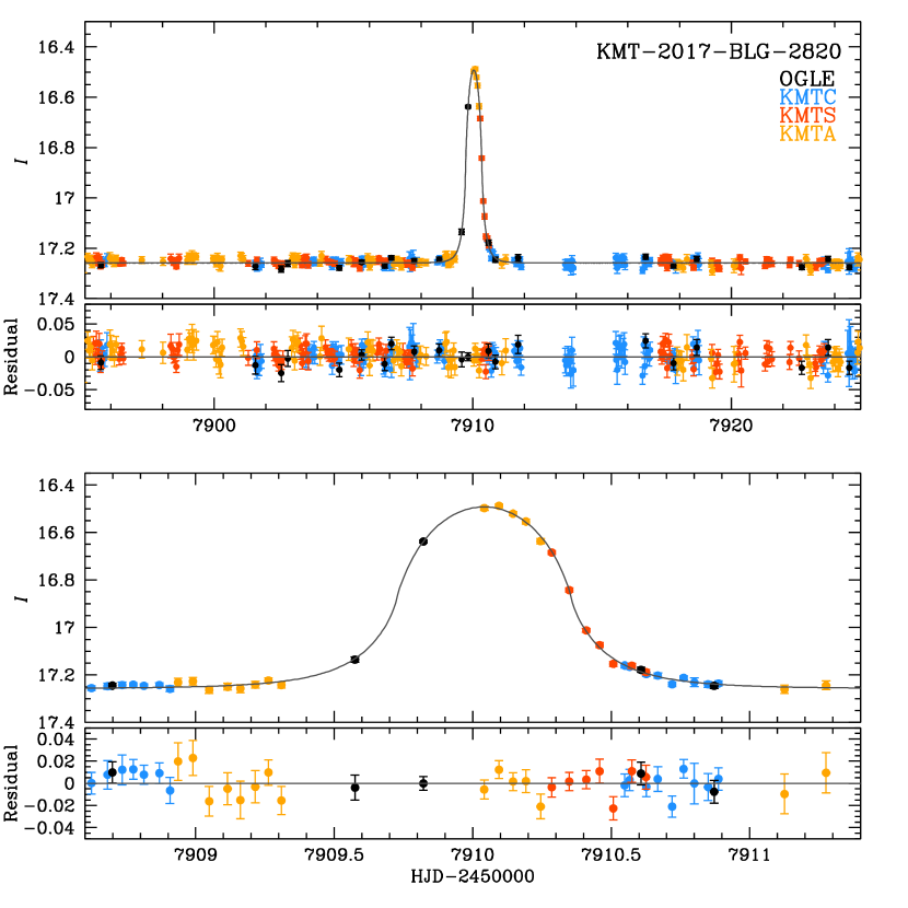
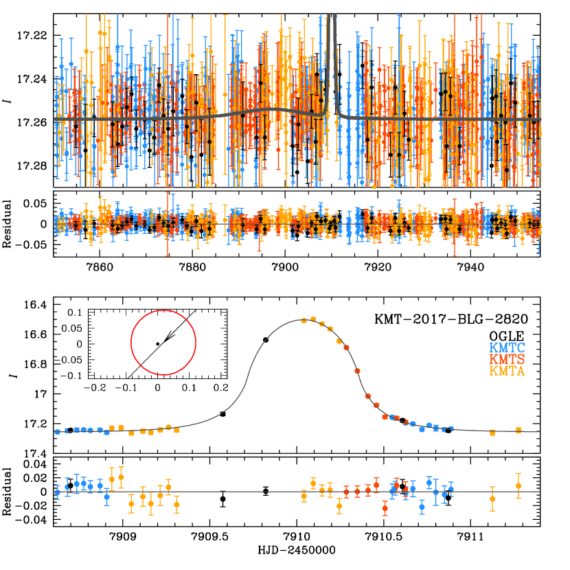
Figure 1 shows the color-coded data from the four observatories together with the best-fit zero-blending FSPL model, which has four parameters (apart from the flux parameters). These are the three Paczyński (1986) parameters and , where is the time of closest approach and is the impact parameter in units of . The fit parameters are given in Table 1. This will be our preferred solution. However, in contrast to the cases of some other FSPL FFP candidates, there is no compelling reason from the light curve data themselves to conclude that the source is unblended. For example, for OGLE-2019-BLG-0551, the blending was poorly constrained, but the source color was well measured to be similar to that of the baseline object. This implied that strong blending was unlikely. But, more importantly, it implied that the determination was independent of the blending (Mróz et al., 2020). The current case is closer to that of KMT-2019-BLG-2073, for which the source color was not measured and the blending fraction was measured to only about at the level (Kim et al., 2020). However, in the present case, while there is also no color measurement and the limit on is similar, there is a strong limit that implies that the source definitely dominates the light from the baseline object. This fact will play an important role in the argument given in Section 6 that the source is most likely not blended.
Before continuing, we remark on the technical point that we implement “zero blending” by fixing i.e., we equate the source and baseline fluxes at KMTA. We find in Section 4 that the color and magnitude offsets of the source from the clump are nearly identical for KMTA and OGLE (and indeed are similar for all four observatories). So, from this standpoint, either (or really, any) observatory could be used. However, the measurement depends primarily on the KMTA data, and is directly proportional to the square root of the normalized surface brightness (Mróz et al., 2020; Kim et al., 2020). Therefore, it is really only the fixing of that directly impacts the result. We considered fixing some or all of the other source fluxes, but this does not significantly change the values of the other parameters compared to just fixing .
Table 1 also shows the parameters for the case of free blending. The estimate of the blended flux is consistent with zero, and the remaining parameters have similar values to the zero-blending fit. However, the errors are much larger. Nevertheless, the normalized surface brightness has a fractional error of only 3.6%, implying that this measurement contributes only 1.8% to the uncertainty in [color term]. That is, as discussed in some detail by Kim et al. (2020), as regards the crucial measurement of , the real uncertainty introduced by unknown blending is the degree to which it implies that the source color differs from that of the baseline object, which is used in the analysis as a proxy for the source color. To address this issue further requires the analysis of two types of auxiliary data: photometric and astrometric.
4 CMD
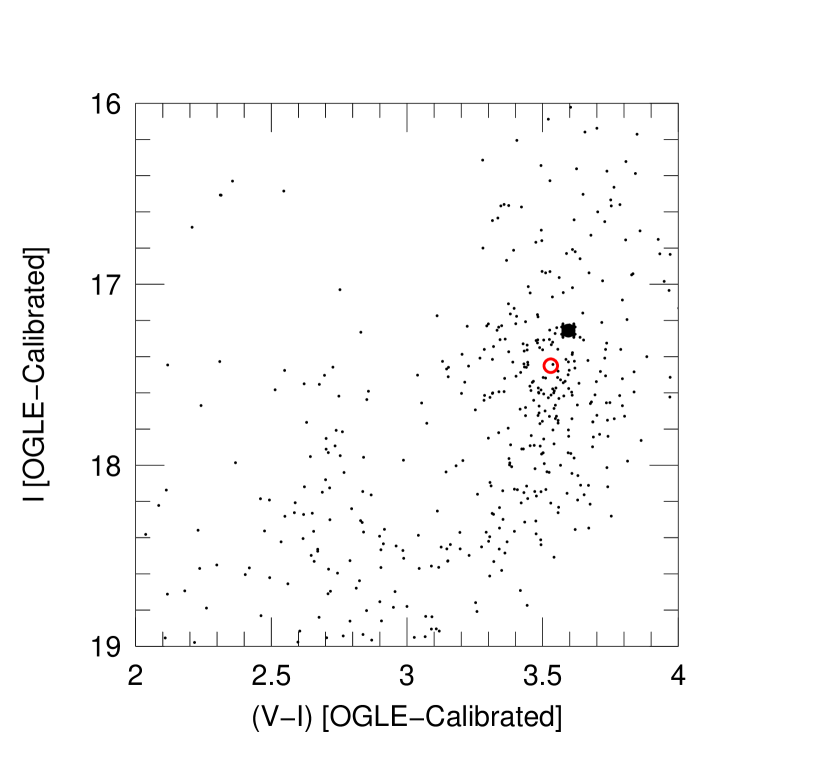
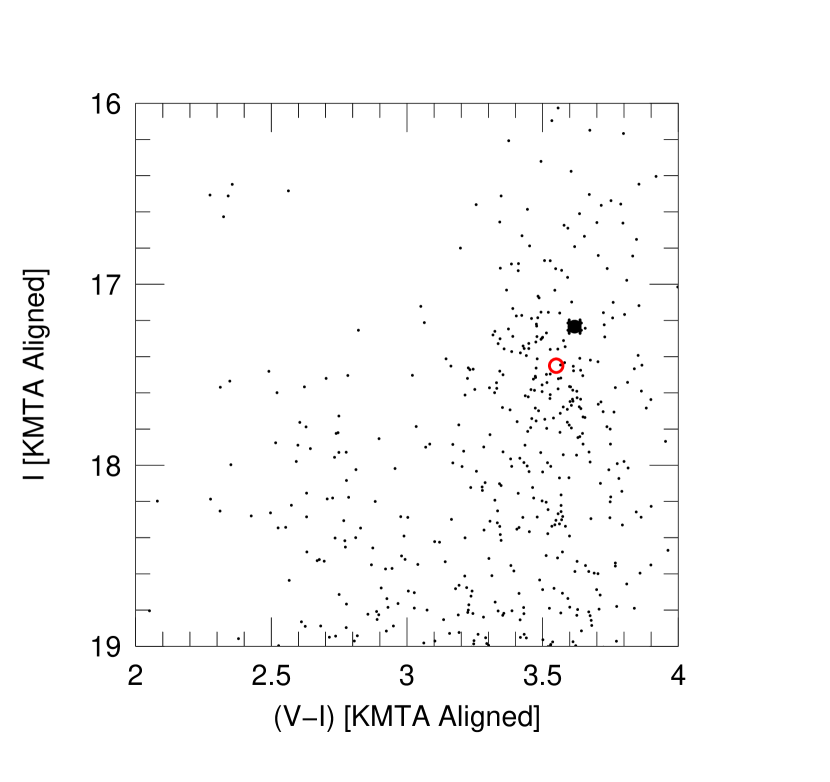
Figures 2 and 3 show color-magnitude diagrams (CMDs) within a box centered on the event for OGLE and KMTA, respectively. In each case, the “baseline object” is shown in black, while the clump centroid is shown in red. The OGLE CMD is calibrated, and the KMTA CMD has been shifted by offsets derived from relatively bright comparison stars, . We need to compare these two CMDs because, while the OGLE photometry is unquestionably better (see, e.g., the lower giant branches in the respective figures), the normalized surface brightness is best constrained from the KMTA data.
We measure the offset from the clump , finding and for OGLE and KMTA, respectively. That is, even though the OGLE photometry is substantially better, the KMTA photometry is adequate for measuring this offset.
In the zero-blending model, the “baseline object” is the source. Then, using the known dereddened position of the clump (Bensby et al., 2013; Nataf et al., 2013), we obtain , where the principal source of error is from centroiding the clump. We cannot use a substantially larger area because of differential reddening. Then employing the standard procedure of Yoo et al. (2004), we convert to using the color-color relations of Bessell & Brett (1988) and apply the color/surface-brightness relation of Kervella et al. (2004) to obtain,
| (4) |
where we have added 5% to the error, in quadrature, to account for systematic errors in the overall method. Using the zero-blending parameters from Table 1, we then obtain
| (5) |
We re-emphasize that Equations (4) and (5) only apply under the assumption of zero blending. However, from the standpoint of measuring , it is equally important to emphasize that this measurement is affected by blending only to the extent that the blend color differs from that of the baseline object. As discussed in Section 3, [color term]. Because is nearly invariant, is unaffected by blending, provided that it does not change the estimated color of the source.
5 Astrometry
If there is blended light that is displaced from the source by , then the source position (measured from difference images near peak) will be displaced from the baseline object by
| (6) |
where is the fraction of the baseline-object flux that is due to the blend. Using the three good seeing images near peak, we measure, in pixels, and in the (West,North) coordinate system of the detector, , where the error bars are the standard errors of the mean of the three measurements. The baseline object position is . While we do not have an independent way to estimate the error bars of this latter measurement, we judge them to be of the same order as those of because the baseline object is bright and isolated and because the baseline flux is similar to the difference flux at peak. Together, these yield
| (7) |
Even assuming Gaussian statistics (which would be somewhat optimistic), this has a probability of under the hypothesis that the true value is zero (i.e., either or ). Hence, the astrometric measurement does not provide positive evidence in favor of blended light, and it is consistent with zero blended light. We now turn to the limits and constraints on blended light.
6 Three Types of Blend
As discussed in Section 3, we have adopted the parameters of the zero-blend fit, even though the light curve permits 20% blending at and 40% at . In this section, we justify this choice.
Logically, there are only three possible sources of blended light: a companion of the source, a companion of the lens, and an ambient star that is unrelated to the event. We consider these in turn.
6.1 Companion of the Source
First we note that the light curve provides only weak constraints on a putative source companion. The Einstein radius is smaller than the source (i.e., ), so a putative companion would not be magnified during the event and would have an extremely low probability of being magnified before or after the event. If the source companion were sufficiently close, it could give rise to a xallarap signal, of which there is no evidence. Because the source is a giant, with , a companion could give rise to ellipsoidal variations over the entire light curve, provided that the source companion were at separations less than a few tenths of an astronomical unit. These are the only constraints on this scenario from the light curve.
Second, the astrometric measurement likewise provides only weak constraints. If a source companion contributed significantly to , which is the only case of interest here, and if it were widely separated from the source, then it would induce an offset between the source and baseline object, which is not seen. For example, for a separation of (i.e., a period of days) and , this would lead to an offset , in contradiction to Equation (6). This implies that the combination of photometric and astrometric constraints leaves open the vast majority of the binary-separation distribution for solar-mass stars (Duquennoy & Mayor, 1991).
However, the prior probability of such a companion is very low, although not completely negligible. To contribute at least of the baseline light, the companion would have to be on the lower giant branch (or possibly in the clump). The baseline-object CMD position corresponds to a roughly solar mass star, and these spend less than 1 Gyr on the lower giant branch, compared to about 10 Gyr on the main sequence. According to Table 7 of Duquennoy & Mayor (1991), less than 10% of solar type stars have companions with mass ratios of 0.75 – 1.00. Therefore, less than 1% of bulge giant stars on the upper giant branch will have companions on the lower giant branch.
Although this probability is very low, we nevertheless now examine the consequences of such a companion for the measurements of and, secondarily, . The main point is that the lower giant branch (and clump) have very similar colors to the baseline object. We therefore begin by asking how these parameters would be affected if the colors were identical. As already noted, because is an invariant, the value of is basically unaffected. Then, because is also an invariant, scales directly as , i.e., , where is the value derived in Section 4 for the zero-blending case. For example, for , the proper motions would be slower by a factor . The major concern raised by such an overestimated would be that, via Equation (1), one should really wait a factor 1.2 times longer before doing AO observations to search for a wide host. Because there will not be any additional information that would rule out such a source companion prior to AO observations, this would mean that one should just wait the extra time (or simply discount the probability that there is such a companion).
However, in fact, for , the source companion would be at least 1.3 mag below the baseline object, and so directly below the clump, which is on average about mag bluer than the baseline object in . Although is a logarithmic quantity, it is small enough that we can treat it as linear in order to get an understanding of its role. Then , and thus the source is redder than the baseline object. And this implies that
| (8) |
where is the source surface brightness as a function of color. We evaluate using the same method that was used in Section 4, and thus obtain
| (9) |
The first point is that the effect is small: for and , , which is less than the statistical error. Second, the impact on the estimated proper motion is opposite in sign from the one identified above when we approximated the source and baseline-object colors as being the same. The combined effect is approximately given by
| (10) |
Thus, the color term only slightly mitigates the color-free term, i.e., by of order .
In summary, there is a very small probability that the source has a companion with sufficient flux to impact the determinations of and . If it does, it changes by substantially less than the statistical error. The fractional change in is larger, but still less than 15%. This might lead one to increase the wait time for AO followup observations, if one were sufficiently concerned about this probability.
6.2 Companion (i.e., Host) of the Lens
We will conduct a search for a host of the planet and thereby place constraints on such a host in Section 8. However, from the present perspective, all that is important about this search is that there will be substantial parameter space, in particular, in the domain of planet-host separation, that is unconstrained.
As we will show immediately below, it is a priori unlikely that the lens contributes to the light of the baseline object at even the level. Nevertheless, the major concern is that the very presence of such a host would prevent its detection in AO followup observations by inducing an underestimate of the wait time. In that case, a non-detection would falsely lead to the conclusion that the lens was an FFP444Note that a BD could also yield a non-detection, provided that , corresponding to pc. While not impossible, this is very unlikely.. However, we will show that there is, in fact, no basis for this concern.
The first point is that if the host is contributing of the baseline-object light, then it must be relatively nearby. Comparing the observed position of the clump (Figure 2) to its intrinsic position (Bensby et al., 2013; Nataf et al., 2013), we derive . At , we estimate that the lens would lie in front of of the dust. Then, to generate , the lens absolute magnitude would be . This excludes essentially all lenses in the bulge and at in the disk from contributing significantly to the blended light, as well as excluding the great majority at somewhat smaller distances.
To understand why blending from the remaining possible lenses cannot undermine the wait-time estimate, we first consider the special case that the (observed) lens color is the same as that of the baseline object. The proper motion will then be overestimated by a factor so that true separation will be (1.42,1.25) FWMH for , rather than 1.5 FWHM. But the flux ratio in (and so in , because the colors are the same), will be . The first would easily be resolved at 1.2 FWHM, while the second would easily be resolved at 1.0 FWHM. See, for example, Figure 1 of Bennett et al. (2020). For lenses that are bluer than the source, the -band flux ratio will be somewhat reduced compared to this estimate. For example, for a solar-like star at , , leading to flux ratios that are a factor roughly (3,2) smaller in band relative to band. However, in these cases, the proper motion will not actually be underestimated because the source is substantially redder than the baseline object. On the other hand, if the source were redder than the baseline object because the lens was an extremely nearby late M dwarf, e.g., , then the proper motion could be underestimated by a factor (0.88,0.65) for , leading to true offsets of (1.3,1.0) FWHM. However, these values would still be adequate even at the -band flux ratio , and the -band ratio would be significantly higher.
The resilience of the wait-time estimate is due to the fact that it was derived to enable lens-flux measurements in the face of extreme flux ratios , whereas blending does not play a significant role unless .
Therefore, there is no real possibility of failure of future AO observations due to adopting the “naive” estimate given in Section 4.
6.3 Ambient Star
The astrometric measurement in Section 5 places strong constraints on blends by ambient stars. We adopt a conservative upper limit, , which leads to an upper limit on the offset of an ambient star at , which covers an area . For , the surface densities of stars with are , with corresponding probabilities . Thus, the probability of an ambient star is small (1.4%), while that of an ambient star is negligible.
6.4 Summary
Among the three possibilities for blended light (companion of the source, companion of the lens, and ambient star), two have both low probability of existing and low impact if they do exist. For both source companion and ambient star, the probability is of order 1% or less. For source companions, the only real scientific impact is that allowing for this possibility suggests to extend the wait time for AO observations by 20%. However, such observations can be taken at first AO light on 30m telescopes, regardless. For ambient stars, only blends have relevant probabilities, and these have only a small impact on the observables and .
If there is a lens companion, then most likely it has . For example essentially all bulge lenses would have hosts with , essentially all disk lenses at would have hosts with , and a large fraction of more nearby hosts would also have . In sum, even if there is a host, the probability that it has is small. Nevertheless, it is quite easy to conjure scenarios of hosts that are above this threshold, as we demonstrated in Section 6.2. However, we also showed there that such hosts would be detected by late-time AO observations regardless of their impact on the proper-motion estimate that was evaluated in Section 4.
7 Source Proper Motion
It is possible in principle to distinguish between bulge and disk lenses by combining the scalar lens-source relative proper motion (derived from the microlensing analysis) with the vector source proper motion derived from external sources. For example, Mróz et al. (2020) found that the source star for OGLE-2016-BLG-1928 had a proper motion almost identical to the centroid of the neighboring bulge field stars. Because in that case, the lens had to be moving at relative to the mean bulge motion. However, the Gaia proper motion diagram showed that there are few, if any, bulge stars with such proper motions.
We pursue a similar investigation here. We use 10 years of OGLE-IV data, which we align to Gaia using a technique that is described by Udalski et al. (2020). We find that the proper motion of the baseline object is
| (11) |
where we have doubled the formal errors derived from the scatter of the fit, based on tests performed by Udalski et al. (2020) in regions where overlapping OGLE fields provide two independent measurements. This measurement agrees with Gaia within the errors, but is more precise. Note that Gaia errors in bulge fields are also underestimated by a factor of about two. In view of the small probability of significant blended light found in Section 6, we identify the source with the baseline object, .
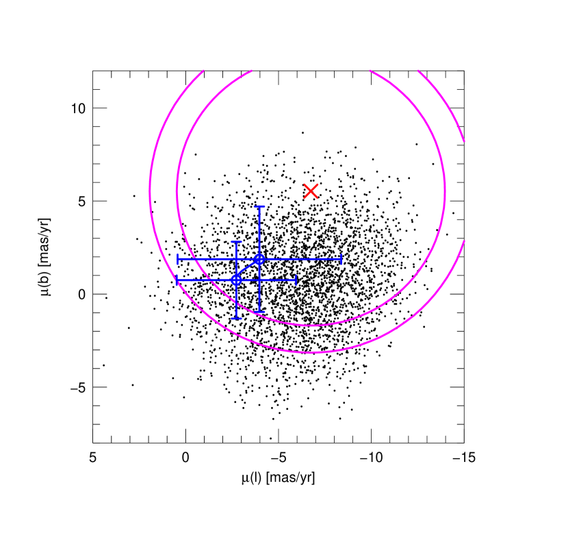
Figure 4 shows this measurement (red), together with the proper motions of bulge field stars (black). The figure is rotated to Galactic coordinates. In addition, for the first time, we show all proper motions in the geocentric frame at the time of the peak of the event, when Earth was moving relative to the Sun. Thus, before rotating the OGLE-IV heliocentric proper motions to Galactic coordinates we first subtract , where .
In this way, we ensure that the magenta circle that is centered on the geocentric source proper motion, and represents the geocentric lens-source relative proper motion, accurately predicts the range of allowed geocentric lens proper motions. Note that to obtain the range of the predicted we have added in quadrature the errors for and . As can be seen, this range is quite consistent with the lens lying in the bulge (black points).
We now ask whether this annulus is also consistent with the lens lying in the disk. The blue circles represent the mean geocentric lens proper motion for disk lenses lying at 2 kpc (right) and 5 kpc (left). The error bars reflect the velocity dispersions of stars at each distance. The blue curve connecting the blue circles shows the mean proper motions at . We have assumed dispersions of where is the ratio of the local surface density to the one in the solar neighborhood. We also assume an asymmetric drift of , where is the local rotation speed. We take account of the motion of the Sun relative to the local standard of rest (LSR), , as well as the instantaneous motion of Earth. The mean estimates for each distance are well displaced toward lower from the origin. Three factors contribute to this. First, the Sun is moving at relative to the LSR in this direction. Second, Earth’s instantaneous motion is relative to the Sun in this direction. Third, the asymmetric drift of stars at these distances is in the opposite direction. In the latitude direction, Earth’s strong motion toward Galactic south overwhelms the small northerly motion of the Sun.
Hence, the mean expected motion is displaced from the origin, though which the magenta annulus directly passes. Nevertheless, after taking account of the velocity dispersions of the lens (error bars), the lens is consistent with being in the disk at the level and at any distance from us. Thus, the proper-motion analysis is quite consistent with the lens lying in either the bulge or the disk.
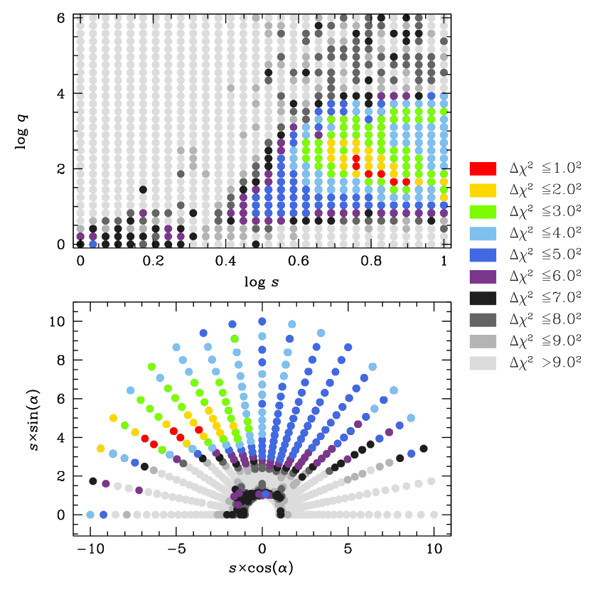
8 2L1S Analysis
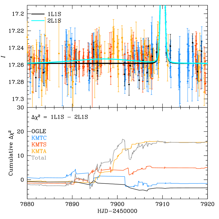
If the lens has a host, then it may leave its signature on the (seemingly) 1L1S event, either by generating a second, much longer, bump in the light curve or by creating caustic structures on the main, short timescale, event. To search for such host signatures, we follow the procedures described by Kim et al. (2020) for KMT-2019-BLG-2073. In particular, we add three parameters to the fit , i.e., the planet-host separation in units of the total-mass (i.e., host+planet) Einstein radius, the ratio of the host and planet masses, and the angle of the host-planet axis with respect to the lens-source relative motion. We center the coordinate system on the planetary caustic. We conduct a grid search in these variables, seeding the remaining four at their values implied by the 1L1S solution. Figure 5 shows the result of this search, with a clear minimum at about , which is favored over the 1L1S solution by . Figure 6 shows the corresponding light curve for the best fit.
To understand the origin of this improvement, we plot the cumulative distribution of in Figure 7. This shows that the net improvement comes entirely from KMTA, with the other three observatories canceling each other out. Hence, the most likely explanation for the improvement is low-level systematics in the KMTA data.
Returning to Figure 5, we see that all models with and have relative to the minimum, and so relative to 1L1S. The same applies to models with and . We regard such models as ruled out. Thus, if future AO observations identify a host, yielding estimates of and , and if second-epoch observations measure the projected planet-host separation (see Section 9.3), then . For example, if and , then , and we predict . As we discuss in Section 9.3, this threshold is near the limit with current instrumentation (and modest efforts), but plausibly could be achieved with 30m AO.
9 Discussion
9.1 Nature of the Observed FFP Population
KMT-2017-BLG-2820 is the sixth FSPL FFP candidate discovered to date. Five of these six (all except OGLE-2016-BLG-1928, which has much smaller and ) have Einstein radii in the range . While these five were not selected homogeneously, they do have some common features that should help us to understand their parent population. First, all five events occurred on giant-star sources with angular radii . Second, all five have Einstein timescales .
This Einstein-timescale range can be directly compared to that of the six PSPL FFP candidates discovered by Mróz et al. (2017), . On this basis, these two samples appear to be drawn from the same underlying population. In the Appendix, we show that the two samples have consistent discovery rates.
We can express the definition of (Equation (2)) as a relation scaled to a value of that is typical of bulge lenses:
| (12) |
Hence, if the five FSPL FFPs lay in the bulge, this population would consist of sub-Jovian gas giants and ice giants. However, even though bulge lenses generally dominate the microlensing event rate, one must be cautious about this interpretation. It is possible, for example, that nature produces very few gas-giant FFPs (or wide separation planets), in which case these low- lenses would mostly or all be in the Galactic disk, with correspondingly lower masses. That is, Equation (12) can equally be written as,
| (13) |
One might hope to distinguish between these alternatives based on the measured (scalar) proper motions, . However, in all five cases, is consistent with either a bulge- or disk-lens interpretation. In principle, if , then a measurement of that put it near the center of the bulge proper-motion distribution can effectively rule out a bulge lens (Mróz et al., 2020). However, for the only one of these five events with , OGLE-2016-BLG-1540, Figure 3 of Mróz et al. (2018) shows that the proper motion of the lens is in fact consistent with it being in either the disk or the bulge.
9.2 The Einstein Desert
Another way to potentially distinguish between the super-Earth/disk and sub-Jovian/bulge hypotheses would be to analyze the full distribution from a homogeneously selected FSPL sample. Under either hypothesis, the observed paucity of short-/small- events555There is only one (OGLE-2016-BLG-1928) out of a total of 12. is explained by declining sensitivity, even if the underlying population of FFPs were rising toward lower mass. However, the two hypotheses make different predictions for the long-/large- tail of the FFP distribution. If these events are due primarily to sub-Jovian/bulge FFPs, then (assuming similar planet formation and evolution in the disk and bulge666Note that in order to contradict the logic of this argument, there would have to be some mechanism that enhanced the production of wide-orbit or unbound sub-Jovian planets in the bulge relative to the disk. For example, the suggestion of Thompson (2013), that gas-giant formation may be suppressed in the bulge due to the harsh radiation environment, would work in the opposite direction. However, McTier et al. (2020) have shown that of bulge stars suffer a stellar encounter within during their 10 Gyr lifetime. Some, but far from all of these would disrupt sub-Jovian gas giants in the cold outer regions. In the impulse approximation, the planet would gain , which is far below its orbital velocity. Here, is the mass of the perturber, is its speed relative to the planet, and is the impact parameter. Thus, to eject the planet (to a wide orbit or out of the system), the star would have to come within of the planet, for which the probability is 100 times smaller.) there should also be a population of sub-Jovian/disk FFPs that give rise to events with roughly times larger and , i.e., centered on days and , respectively. However, is very nearly at the (logarithmic) center of the “gap” found by Kim et al. (2020) in the interval , which we dub the “Einstein desert”. And days is close to the minimum of Figure 1 of Mróz et al. (2017).
In contrast to the sub-Jupiter/bulge hypothesis, the Einstein desert is a natural consequence of the super-Earth/disk hypothesis, which predicts that there are no ejected planets (whether arriving in very wide or unbound orbits) that are more massive than super-Earths. In this scenario, there are no events with intermediate or from the disk (due to non-existence of sub-Jovian FFPs), and very few (or no) FFP events from the bulge (due to the and of super Earths having very low detection sensitivity).
While the Mróz et al. (2017) PSPL sample was selected according to homogeneous criteria, the five FSPL events that we have just been discussing are inhomogeneously selected. However, Kim et al. (2020) presented a plan for collecting a homogeneous sample of giant-source FSPL events, within which the FFP subsample could be analyzed. They applied this approach to 2019 KMT data and found two FFP candidates among their 13 FSPL events. KMT-2017-BLG-2820 was found by applying the same approach to 2017 and 2018 data. It is therefore the third FFP candidate found in this developing homogeneous sample. The analysis of the 2017–2018 FFP events is ongoing, and it will be extended to 2016 as well. If the Einstein desert remains parched in this expanded sample of FSPL events (as indicated by a preliminary analysis), then this will tend to confirm the super-Earth/disk hypothesis. On the other hand, if this “desert” were gradually populated by intermediate lenses, then the sub-Jovian/bulge hypothesis would gain traction.
9.3 Free-Floating versus Wide-Orbit Planets
As with all FSPL FFPs candidates, one can distinguish between the FFP and wide-orbit scenarios for KMT-2017-BLG-2820 by imaging the system at high resolution when the source and lens are sufficiently separated to be resolved. From Equations (1) and (5), this will be in 2028 or 2026 for Keck AO observations in or , respectively. Or one might be slightly more conservative to allow for the measurement errors in , or concerns about systematic errors in due to unrecognized blending. However, we have argued that the latter concern is minor.
If the planet has a host, then the host should appear in these observations with a separation approximately given by , where is the elapsed time since the event. It will then be possible to determine or constrain the planet-host projected separation by taking a second observation several years later (Gould, 2016). That is, suppose that the two measurements of the offset between the host and source are taken and after the event, each with precision . Then the host position at the time of the event is given by
| (14) |
For example, for (e.g., Vandorou et al. 2020), yr, yr, and a lens distance of , the error corresponds to . This approach only works for planet-host separations that are small compared to the FWHM, i.e., 55 mas for our fiducial parameters, corresponding to for . For separations that are of order the FWHM, the host will appear in some random position that is inconsistent with the one predicted from . Then the host would be identified as such because it moved with the proper motion derived from the microlensing fit between the two epochs. At sufficiently large separations, the method becomes limited by a background of stars moving with similar proper motions. Gould (2016) discusses the problem of distinguishing among “Kuiper, Oort, and Free-Floating Planets” in greater detail.
On the other hand, if no host is seen, this does not absolutely prove that the lens is an FFP. As mentioned, it could be a BD that passed in front of the source. Or it could have a dark host, such as a BD, old white dwarf, neutron star, or black hole. However, while these rare exotic systems might explain one non-detection, they could not explain an ensemble of non-detections.
While there is no purely empirical evidence that would distinguish between the FFP and wide-orbit explanations for the FFP candidates, the balance of evidence from a combination of theoretical arguments and observational data strongly favors the FFP hypothesis.
First, as we have described above, the existence of the “Einstein desert” implies that these lenses are super-Earths in the disk rather than gas giants in the bulge. While this desert must be confirmed, we can report that with most of the FSPL analysis of 2017-2019 complete, the desert remains.
Second, to account for their six detected PSPL FFP candidates, Mróz et al. (2017) required 5–10 times more FFP super-Earths than stars. Given the typical lower limits on hosts, adopting typical distances for disk lenses, and adopting for the snow line, this would imply projected separations, , relative to the snow line, i.e., beyond the orbit of Jupiter in the Solar System. There could easily be one super-Earth in this zone, but if there are 5–10 per star, then they must be spread to considerably larger orbits. For the Solar System, it is well established that the timescales in these regions are too slow to form super-Earths.
Therefore, in the wide-orbit hypothesis, the super Earths must have formed closer in and then been “ejected” from these inner regions to where they are seen today. There is, indeed, the well worked out “Nice model” (Tsiganis et al., 2005) for such an ejection to explain the present positions of Uranus and Neptune. This model must (and does) explain how these planets retained their roughly circular orbits, but it relies on a Jupiter-Saturn resonance. Such two-gas-giant systems are relatively rare (Gould et al., 2010; Wittenmyer et al., 2020). Hence, more generally, “mass expulsions” (i.e., 5–10 planets) would take place by planet-planet scattering, or pumping (as created the Oort cloud) that would send the planets into highly elliptical orbits. If the mechanism were scattering, it would require fine tuning to have the planets lose most of their energy, but remain bound. This already implies that FFP and Oort-like orbits should predominate over Kuiper-like orbits. Moreover, in the process of the super-Earth migration to pumping orbits, it seems likely that most would be scattered out of the system.
As we have emphasized, it will be possible to test these conjectures by AO followup to locate hosts, and by second-epoch AO to determine their separations.
10 Conclusion
We have discovered a new FSPL FFP candidate, KMT-2017-BLG-2820, with Einstein radius and lens-source relative proper motion . Whether this is truly a “free-floating planet” or is simply a very wide-separation planet can can be determined with excellent (though not perfect) confidence by AO followup observations made before the end of the current decade. If the latter, then the planet-host projected separation can be measured with roughly precision from a second AO epoch.
KMT-2017-BLG-2820 was discovered in an ongoing systematic search for giant-source FSPL events within 2016–2019 KMT data (Kim et al., 2020). It is the third FFP candidate in this developing homogeneous sample and the sixth FSPL FFP candidate overall. Five of these six FSPL FFP candidates have a very similar Einstein timescale distribution as the six PSPL FFP candidates found by Mróz et al. (2017) in their study of 1L1S events found in the OGLE-IV database. Moreover, the detection rates of the Mróz et al. (2017) PSPL sample and the sample being collected under the Kim et al. (2020) protocols are comparable (see Appendix). We therefore argue that the five FSPL FFP candidates and six PSPL FFP candidates are drawn from the same population. Based on the measured Einstein radii of the former, these could be either sub-Jovian FFPs in the bulge or super-Earth FFPs in the disk. We argue that, if the Einstein desert in the distribution of giant-source FSPL events tentatively found by Kim et al. (2020) is confirmed, then it argues for the latter scenario, which was already suggested by (Mróz et al., 2017) on different grounds.
In making our parameter estimates, we have adopted the zero-blending model. First, while the blending parameter is relatively weakly constrained by the light curve at the level, , it has a firm upper limit at the level. Thus, the source dominates the baseline object, which sits on the upper giant-branch track. Hence, the probability for from a source companion is less than 1% due to rarity of lower giant-branch stars. The probability for from an ambient star is similarly restricted by the close astrometric alignment between the source and the baseline object. If the lens has a host, then this would supply blended light at some level. However, essentially all potential hosts at generate and this applies to most potential hosts at as well. In any case, we showed that ignoring such possible blended light from the host would not cause one to overestimate and thereby underestimate the wait time for AO followup observations.
Appendix A Relative Rates of the PSPL and FSPL FFP Samples
We show here that the detection rates underlying the six Mróz et al. (2017) PSPL sample and the three FSPL events obtained so far under the program outlined by Kim et al. (2020) are roughly comparable. Because Kim et al. (2020) have not yet characterized their selection function, we adopt a basically empirical approach. And because the Poisson errors of this comparison are roughly , there is not much to be gained by detailed, highly precise calculations. We therefore seek only to demonstrate rough consistency.
Mróz et al. (2017) searched nine OGLE fields over about 5.5 seasons, three with cadence and six with cadence . They showed that their detection efficiency in the timescale range of the actual detections was about two times higher in the former. Hence, if the fields had equal underlying rates, there should be a nearly equal number of detections in the two sets of fields. Instead, there are five and one. Some of this difference is due to lower underlying rates in the lower-cadence fields. And some may be due to Poisson fluctuations. Nevertheless, in order to maintain a homogeneous empirical approach, we restrict attention to the three higher-cadence fields, with total area . For simplicity we label the six events shown in Figure 3 and Table 1 of Mróz et al. (2017) as M-1 … M-6. We note that apart from M-1 (which has a giant source), all six have . We therefore estimate the effective cross section as , where we have used based on the ensemble of FSPL FFPs (excluding OGLE-2016-BLG-1928, which has a timescale outside the range of either the Mróz et al. 2017 sample or that of the Kim et al. 2020 approach). We estimate the source absolute magnitudes using from Table 1, extinctions from Gonzalez et al. (2012) (with ), and Galactic-bar distances from Nataf et al. (2013). Apart from M-6 (which is also the only event with ), the events all have . We judge this to be the range of source sensitivity.
Based on Figure 8 of Kim et al. (2020), we estimate that the FSPL FFP sample has sensitivity to sources . From their Figure 4, the cross section for the FSPL events is . From Figure 8 (and keeping in mind that for a clump giant, ) we adopt and so a cross section of . As discussed by Kim et al. (2020), and illustrated by their Figure 5, their FSPL search is about equally sensitive in all fields . This is fundamentally because giant-source events have a full duration of about 20 hours. However, as also shown by their Figure 5, detections are dominated by events near the Galactic plane. Although extinction is higher in the northern bulge, this does not affect the relative detection rate much, again because the sources are giants. We judge the effective area of the search to be .
To estimate the relative detection rates, we combine four factors: 1: effective number of sources, 2: effective area, 3: effective cross section, 4: mean diurnal time coverage. We estimate ratios (FSPL/PSPL) . This can be compared to the actual rates of 3/(3 yr) and 5/(5.5 yr) for FSPL and PSPL respectively. The estimate of the first factor is based on the Holtzman et al. (1998) luminosity function (and the effective limits). The second and third factors were described above. The fourth factor derives from the fact that OGLE is operating from a single site, while KMT is operating from three sites, one of which (KMTS) has somewhat worse weather and one of which (KMTA) has substantially worse weather.
The fact that the “predicted” FSPL/PSPL ratio (1.0) and the observed ratio (1.1) are nearly identical should not be over-interpreted: the comparison has no physical meaning below the Poisson errors. In addition, our estimates have considerable uncertainties (although below the Poisson errors). The only aim of this Appendix has been to demonstrate that the two samples are consistent in terms of detection rate.
References
- Alard & Lupton (1998) Alard, C. & Lupton, R.H.,1998, ApJ, 503, 325
- Albrow et al. (2009) Albrow, M. D., Horne, K., Bramich, D. M., et al. 2009, MNRAS, 397, 2099
- Bennett et al. (2020) Bennett, D.P., Bhattacharya, A., Beaulieu, J.-P., et al. 2020, AJ, 159, 68
- Bensby et al. (2013) Bensby, T. Yee, J.C., Feltzing, S. et al. 2013, A&A, 549A, 147
- Bessell & Brett (1988) Bessell, M.S., & Brett, J.M. 1988, PASP, 100, 1134
- Duquennoy & Mayor (1991) Duquennoy, A., & Mayor, M. 1991, A&A, 248, 485
- Gonzalez et al. (2012) Gonzalez, O. A., Rejkuba, M., Zoccali, M., et al. 2012, A&A, 543, A13
- Gould (2016) Gould, A. 2016, JKAS, 49, 123
- Gould et al. (2010) Gould, A., Dong, S., Gaudi, B.S. et al. 2010, ApJ, 720, 1073
- Han et al. (2017) Han, C., Udalski, A., Gould, A. 2017, AJ, 154, 133
- Holtzman et al. (1998) Holtzman, J.A., Watson, A.M., Baum, W.A., et al. 1998, AJ, 115, 1946
- Johnson et al. (2020) Johnson, S.A., Penny, M., Gaudi, B.S., et al. 2020, AJ, 160, 123
- Kervella et al. (2004) Kervella, P., Thévenin, F., Di Folco, E., & Ségransan, D. 2004, A&A, 426, 297
- Kim et al. (2016) Kim, S.-L., Lee, C.-U., Park, B.-G., et al. 2016, JKAS, 49, 37
- Kim et al. (2018) Kim, D.-J., Kim, H.-W., Hwang, K.-H., et al., 2018, AJ, 155, 76
- Kim et al. (2020) Kim, H.-W., Hwang, K.-H., Gould, A., et al. 2020, AAS submitted, arXiv:2007.06870
- McTier et al. (2020) McTier, M.A.S., Kipping, D.M., & Johnston, K. 2020, MNRAS, 495, 2105
- Mróz et al. (2017) Mróz, P., Udalski, A., Skowron, J., et al. 2017, Nature, 548, 183
- Mróz et al. (2018) Mróz, P., Ryu, Y.-H., Skowron, J., et al. 2018, AJ, 155, 121
- Mróz et al. (2019) Mróz, P., Udalski, A., Bennett, D.P.., et al. 2019, A&A, 622, A201
- Mróz et al. (2020) Mróz, P., Poleski, R., Han, C., et al. 2020, AJ, 159, 262
- Mróz et al. (2020) Mróz, P., , Poleski, R., Gould, A., et al. 2020, ApJ, in press, arXiv:2009.12377
- Nataf et al. (2013) Nataf, D.M., Gould, A., Fouqué, P. et al. 2013, ApJ, 769, 88
- Paczyński (1986) Paczyński, B. 1986, ApJ, 304, 1
- Poleski et al. (2014) Poleski, R., Skowron, J., Udalski, A., et al. 2014, ApJ, 755, 42
- Poleski et al. (2017) Poleski, R., Udalski, A., Bond, I.A., et al. 2017, A&A, 604A, 103
- Poleski et al. (2018) Poleski, R., Gaudi, B.S., Udalski, A. et al. 2018, AJ, 156, 104
- Poleski et al. (2020) Poleski, R., et al., 2020, in prep
- Shvartzvald et al. (2017) Shvartzvald, Y., Bryden, G.,Gould, A. et al. 2017, AJ, 135, 61
- Sumi et al. (2011) Sumi, T., Kamiya, K., Bennett, D. P., et al. 2011, Nature, 473, 349
- Thompson (2013) Thompson, T.A. 2013, MNRAS, 431, 63
- Tomaney & Crotts (1996) Tomaney, A.B. & Crotts, A.P.S. 1996, au, 112, 2872
- Tsiganis et al. (2005) Tsiganis, K., Games, R., Morbidelli & Levison, H.F. 2005, Natur, 435, 459
- Udalski (2003) Udalski, A. 2003, Acta Astron., 53, 291
- Udalski et al. (1994) Udalski, A.,Szymanski, M., Kaluzny, J., Kubiak, M., Mateo, M., Krzeminski, W., & Paczyński, B. 1994, Acta Astron., 44, 227
- Udalski et al. (2020) Udalski, A. et al. (2020) in prep.
- Vandorou et al. (2020) Vandorou, A., Bennett, D.P., Beaulieu, J.-P., et al., 2020, AJ, 150, 121
- Wittenmyer et al. (2020) Wittenmyer, R.A., Want, S. Horner, J., et al. 2020, MNRAS, 492, 377
- Woźniak (2000) Woźniak, P. R. 2000, Acta Astron., 50, 421
- Yoo et al. (2004) Yoo, J., DePoy, D.L., Gal-Yam, A. et al. 2004, ApJ, 603, 139
| Parameters | 1L1S | 1L1S [=2.06] |
|---|---|---|
| 1994.017/1994 | 1994.645/1995 | |
| 7910.046 0.009 | 7910.043 0.007 | |
| 0.164 0.105 | 0.302 0.053 | |
| 0.288 0.015 | 0.273 0.006 | |
| 1.096 0.079 | 1.187 0.009 | |
| 0.314 0.010 | 0.324 0.006 | |
| 1.503 0.054 | 1.465 0.023 | |
| 1.805 0.204 | 2.06 | |
| 0.252 0.204 | -0.003 0.001 | |
| 1.736 0.165 | 1.939 0.085 | |
| 0.244 0.165 | 0.042 0.085 |
Note. — and are derived quantities and are not fitted independently.