Koopman-Based Learning of Infinitesimal Generators
without Operator Logarithm

Given a pre-compact state space $\mathcal{X}\subseteq\mathbb{R}^{n}$, we consider a continuous-time nonlinear dynamical system of the form

where $x$ denotes the initial condition, and the vector field $f:\mathcal{X}\rightarrow\mathcal{X}$ is assumed to be locally Lipschitz continuous. We denote by $\phi:\mathcal{I}\times\mathcal{X}\rightarrow\mathcal{X}$ the forward flow, also known as the solution map.

The evolution of observable functions of system (1) restricted to $C(\mathcal{X})$ is governed by the family of Koopman operators, defined by

for each $t\geq 0$, where $\circ$ is the composition operator. By the properties of the flow map, it can be easily verified that $\left\{\mathcal{K}_{t}\right\}_{t\geq 0}$ forms a semigroup, with its (infinitesimal) generator defined by

Within the space of continuous observable functions, the limit in Eq. (3) exists on the subspace of all continuously differentiable functions, indicating that $\operatorname{dom}(\mathcal{L})=C^{1}(\mathcal{X})$. In this case, we can verify that the generator of Koopman operators is such that

Note that the finite-difference method [22, 23, 24] indirectly approximates the generator by setting a small terminal time without taking the limit on the r.h.s. of (3). Through this approximation scheme of the time derivative, it can be anticipated that the precision heavily depends on the size of that terminal time.

If $\mathcal{L}$ is a bounded linear operator that generates $\{\mathcal{K}_{t}\}$, then $\mathcal{K}_{t}=e^{t\mathcal{L}}$ for each $t$ in the uniform (operator) topology. However, many of the differential operators that occur in mathematical physics are unbounded. We revisit some concepts to show how to interpret $\mathcal{K}_{t}$ in terms of the possibly unbounded generator on an exponential scale.

We further define the Yosida approximation of $\mathcal{L}$ as

Note that $\left\{\mathcal{L}_{\lambda}\right\}_{\lambda\in\rho(\mathcal{L})}$ is a family of bounded linear operators, and $e^{t\mathcal{L}_{\lambda}}$ is well-defined for each $\lambda\in\rho(\mathcal{L})$.

Let $C(\mathcal{X})$ be endowed with the uniform norm $|\cdot|_{\infty}:=\sup_{x\in\mathcal{X}}|\cdot|$. Suppose that $\{\mathcal{K}_{t}\}_{t\geq 0}$ is a contraction semigroup where

for all $t\geq 0$. Then, $\rho(\mathcal{L})\supseteq(0,\infty)$, and by [25, Lemma 1.3.3], we have that $\left\{\mathcal{L}_{\lambda}\right\}_{\lambda>0}$ converges strongly to $\mathcal{L}$. Specifically, when working on the $C^{2}(\mathcal{X})$ subspace, the convergence rate is given by $\mathcal{O}(\lambda^{-1})$.

To address more general cases, we first present the following facts.

Intuitively, $M$ represents the uniform scaling of the magnitude of the Koopman operator, while $\omega$ indicates the dominant exponential growth or decay rate of the flow on $C(\mathcal{X})$. The above properties provide us with a tool to convert the dominant exponential growth or decay rate of the flow on $C(\mathcal{X})$ by introducing an extra term $\lambda\operatorname{I}$ to the original generator. Specifically, the transformation $e^{-\omega t}\mathcal{K}_{t}$ allows us to work in a topology (by shifting the direction of flows and uniformly compressing by $M$) that is equivalent to the uniform topology of continuous functions, where the semigroup $\{e^{-\omega t}\mathcal{K}_{t}\}$ is a contraction. The convergence of $\mathop{\mathrm{s\text{-}\lim}}_{\lambda\rightarrow\infty}\mathcal{L}_{\lambda}=\mathcal{L}$ for $\left\{\mathcal{L}_{\lambda}\right\}_{\lambda>\omega}$ and its reciprocal convergence rate can similarly be demonstrated in this new topology.

Motivated by representing $\mathcal{L}$ by $\left\{\mathcal{K}_{t}\right\}_{t\geq 0}$ and the Yosida approximation for $\mathcal{L}$ on $\{\lambda>\omega\}$, we establish a connection between $R(\lambda;\mathcal{L})$ and $\left\{\mathcal{K}_{t}\right\}_{t\geq 0}$.

Restricted to the $C^{1}(\mathcal{X})$ subspace, to use the approximation in Section III-A, we can replace $R(\lambda;\mathcal{L})$ with $R(\lambda)$.

The current form of the improper integral in (7) cannot be directly used for a data-driven approximation. We need to further derive an approximation approach based on finite-horizon observable data. Below, we present a direct truncation modification based on (7).

It can be shown that for any $\lambda$, the truncation in Definition III.4 results in an error term $e^{-\lambda\tau}R(\lambda)h(\phi(\tau,x))$ that is uniformly bounded for each observable function $h$, with the dominant term being $e^{-\lambda\tau}$. This indicates that for any arbitrarily large $\lambda$, this truncation does not significantly affect the accuracy compared to the procedure from $\mathcal{L}_{\lambda}$ to $\mathcal{L}$.

For any fixed $\tau>0$, we can therefore use

to approximate $\mathcal{L}$ within a small time-horizon. We illustrate this approximation with the following simple example.

For any fixed $\lambda>0$, given a dictionary $\mathcal{Z}_{N}$ of the form (10), for each $\mathfrak{z}_{i}\in\mathcal{Z}_{N}$ and each $x\in\mathcal{X}$, we consider $\mathfrak{z}_{i}(x)$ as the features and $\lambda^{2}\mathcal{T}_{\tau}\mathfrak{z}_{i}(x)-\lambda\mathfrak{z}_{i}(x)=\lambda^{2}\int_{0}^{\tau}e^{-\lambda s}\mathfrak{z}_{i}(\phi(s,x))ds-\lambda\mathfrak{z}_{i}(x)$ as the labels. To compute the integral, we employ numerical quadrature techniques for approximation. This approach inevitably requires discrete-time observations (snapshots), the number of which is denoted by $\mathbf{N}$, within the interval $[0,\tau]$ of the flow map $\phi(\tau,x)$.

To streamline the evaluation process for numerical examples, drawing inspiration from [27], for any $\tau$ and $i$, we can assess both the trajectory and the integral, i.e. the pair $\left(\phi(\tau,x),\lambda^{2}\int_{0}^{\tau}e^{-\lambda s}\mathfrak{z}_{i}(\phi(s,x))ds\right)$, by numerically solving the following augmented ODE system

We summarize the algorithm for generating training data for one time period as in Algorithm 1.

After obtaining the training data $(\mathfrak{X},\mathfrak{Y})$ using Algorithm 1, we can find $\mathbf{L}$ by $\mathbf{L}=\operatorname{argmin}_{A\in\mathbb{C}^{N\times N}}\|\mathfrak{Y}-\mathfrak{X}A\|_{F}$. The $\mathbf{L}$ is given in closed-form as $\mathbf{L}=\left(\mathfrak{X}^{T}\mathfrak{X}\right)^{\dagger}\mathfrak{X}^{T}\mathfrak{Y}$, where $\dagger$ is the pseudo inverse. Similar to Extended Dynamic Mode Decomposition (EDMD) [26] for learning Koopman operators, the approximations (11) and (12) can be guaranteed. In addition, by the universal approximation theorem, all of the function approximations from above should have uniform convergence to the actual quantities.

It is worth noting that operator learning frameworks, such as autoencoders, which utilize neural networks (NN) as dictionary functions, can reduce human bias in the selection of these functions [5]. Incorporating the proposed learning scheme with NN falls outside the scope of this paper but will be pursued in future work.

The actual vector field is

As we can analytically establish that $\mathcal{L}\mathfrak{z}_{1,0}(x)=f_{1}(x)$ and $\mathcal{L}\mathfrak{z}_{0,1}(x)=f_{2}(x)$, we use the approximation $[\widetilde{\mathcal{L}}_{\lambda}\mathfrak{z}_{1,0},\widetilde{\mathcal{L}}_{\lambda}\mathfrak{z}_{0,1}]$ to conversely obtain $f$.

Note that $\mathfrak{z}_{1,0}(x)=\mathcal{Z}_{N}(x)\mathbf{e}_{2}$ and $\mathfrak{z}_{0,1}(x)=\mathcal{Z}_{N}(x)\mathbf{e}_{5}$, where each $\mathbf{e}_{i}$ for $i\in\left\{0,1,\cdots,N\right\}$ is a column unit vector with all components being $0$ except for the $i$-th component, which is $1$. To apply $\mathbf{L}$, we have that $\widetilde{\mathcal{L}}_{\lambda}\mathfrak{z}_{1,0}(x)\approx\mathcal{Z}_{N}(x)(\mathbf{L}\mathbf{e}_{2})$ and $\widetilde{\mathcal{L}}_{\lambda}\mathfrak{z}_{0,1}(x)\approx\mathcal{Z}_{N}(x)(\mathbf{L}\mathbf{e}_{5})$.

In other words, we approximate $\widetilde{\mathcal{L}}_{\lambda}\mathfrak{z}_{1,0}$ and $\widetilde{\mathcal{L}}_{\lambda}\mathfrak{z}_{0,1}$ (and hence $f_{1}$ and $f_{2}$) using a linear combination of functions within $\mathcal{Z}_{N}$. The weights for these approximations are given by $\mathbf{L}\mathbf{e}_{2}$ and $\mathbf{L}\mathbf{e}_{5}$, respectively. We report the corresponding results in Table I and II.

We compare the aforementioned results with those obtained using the benchmark approach as described in [16] with the same $M$ and $\mathcal{Z}_{N}$. As described in Remark IV.1, $\mathbf{K}\in\mathbb{C}^{N\times N}$ can be obtained such that $\mathcal{K}_{s}\mathfrak{z}_{1,0}(x)\approx\mathcal{Z}_{N}(x)(\mathbf{K}\mathbf{e}_{2})$ and $\mathcal{K}_{s}\mathfrak{z}_{0,1}(x)\approx\mathcal{Z}_{N}(x)(\mathbf{K}\mathbf{e}_{5})$. Then, we have the approximation, as claimed by [16], $f_{1}(x)\approx\mathcal{Z}_{N}(x)(\log(\mathbf{K})\mathbf{e}_{2}/s)$ and $f_{2}(x)\approx\mathcal{Z}_{N}(x)(\log(\mathbf{K})\mathbf{e}_{5}/s)$ w.r.t. $|\cdot|_{\infty}$. According to [16, Section VI.A], we set $s=0.5$ to avoid the multi-valued matrix logarithm. We report the weights obtained by taking the real parts of $\log(\mathbf{K})\mathbf{e}_{2}/s$ and $\log(\mathbf{K})\mathbf{e}_{5}/s$ in Table III and IV, respectively. Multiple orders of magnitude in accuracy have been established using the proposed method.

It is worth noting that, unlike the experiment in [16] where $i,j\in\left\{0,1,2,3\right\}$, we deliberately choose different numbers for $i$ and $j$, leading to non-negligible imaginary parts after taking the matrix logarithm of $\mathbf{K}$. The imaginary parts of the learned weights using the Koopman-logarithm approach are reported in Table V and VI. The presence of non-negligible imaginary parts indicates that the underlying system is sensitive to the selection of dictionary functions when employing the Koopman-logarithm approach, an effect that is significant and cannot be overlooked when aiming to minimize human intervention in identifying unknown systems in practice. Furthermore, the original experiment in [16] used $M=300^{2}$ samples for a data fitting, and when $M$ is reduced to $100^{2}$, the quality of the operator learning deteriorates.

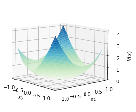
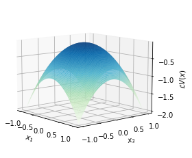
Observing the identified system dynamics, we anticipate that the time-reversed system is (locally) asymptotically stable w.r.t. the origin. We use the learned $\mathbf{L}$ to construct polynomial Lyapunov functions based on the Lyapunov equation $\mathcal{L}V(x)=|x|^{2}$, where the sign on the r.h.s. is reversed due to the dynamics being reversed. To use $\mathbf{L}$ and the library functions from $\mathcal{Z}_{N}$, we define the weights as $\theta:=[\theta_{0},\theta_{1},\cdots,\theta_{N-1}]^{T}$ and seek a $\theta$ such that $V(x;\theta):=\mathcal{Z}_{N}(x)\theta$ , with the objective of minimizing $|\mathcal{Z}_{N}(x)\mathbf{L}\theta-x_{1}^{2}-x_{2}^{2}|$. Ignoring the small terms of the magnitude $10^{-9}$, the constructed Lyapunov function is given by

Additionally, $\mathcal{L}V(x;\theta)$ is approximated by $\mathcal{Z}_{N}(x)\mathbf{L}\theta$, with the maximal value observed at $\mathcal{Z}_{N}(0)\mathbf{L}\theta=-0.068$, which indicates that stability predition using the data-driven Lyapunov function is verified to be valid. This indicates that the stability prediction, as inferred using the data-driven Lyapunov function, is verified to be valid. The visualization can be found in Fig 1.

References

- [1] J. Sjöberg, Q. Zhang, L. Ljung, A. Benveniste, B. Delyon, P.-Y. Glorennec, H. Hjalmarsson, and A. Juditsky, “Nonlinear black-box modeling in system identification: a unified overview,” Automatica, vol. 31, no. 12, pp. 1691–1724, 1995.
- [2] R. Haber and H. Unbehauen, “Structure identification of nonlinear dynamic systems—a survey on input/output approaches,” Automatica, vol. 26, no. 4, pp. 651–677, 1990.
- [3] A. Mauroy and I. Mezić, “A spectral operator-theoretic framework for global stability,” in 52nd IEEE Conference on Decision and Control, pp. 5234–5239, IEEE, 2013.
- [4] A. Mauroy and I. Mezić, “Global stability analysis using the eigenfunctions of the Koopman operator,” IEEE Transactions on Automatic Control, vol. 61, no. 11, pp. 3356–3369, 2016.
- [5] S. A. Deka, A. M. Valle, and C. J. Tomlin, “Koopman-based neural lyapunov functions for general attractors,” in 61st Conference on Decision and Control (CDC), pp. 5123–5128, IEEE, 2022.
- [6] J. L. Proctor, S. L. Brunton, and J. N. Kutz, “Dynamic mode decomposition with control,” SIAM Journal on Applied Dynamical Systems, vol. 15, no. 1, pp. 142–161, 2016.
- [7] Y. Meng, R. Zhou, and J. Liu, “Learning regions of attraction in unknown dynamical systems via Zubov-Koopman lifting: Regularities and convergence,” arXiv preprint arXiv:2311.15119, 2023.
- [8] I. M. Mitchell, A. M. Bayen, and C. J. Tomlin, “A time-dependent Hamilton-Jacobi formulation of reachable sets for continuous dynamic games,” IEEE Transactions on Automatic Control, vol. 50, no. 7, pp. 947–957, 2005.
- [9] Y. Lin, E. D. Sontag, and Y. Wang, “A smooth converse lyapunov theorem for robust stability,” SIAM Journal on Control and Optimization, vol. 34, no. 1, pp. 124–160, 1996.
- [10] J. Liu, Y. Meng, M. Fitzsimmons, and R. Zhou, “Physics-informed neural network lyapunov functions: Pde characterization, learning, and verification,” arXiv preprint arXiv:2312.09131, 2023.
- [11] Y. Meng, Y. Li, M. Fitzsimmons, and J. Liu, “Smooth converse Lyapunov-barrier theorems for asymptotic stability with safety constraints and reach-avoid-stay specifications,” Automatica, vol. 144, p. 110478, 2022.
- [12] Y. Meng and J. Liu, “Lyapunov-barrier characterization of robust reach–avoid–stay specifications for hybrid systems,” Nonlinear Analysis: Hybrid Systems, vol. 49, p. 101340, 2023.
- [13] S. L. Brunton, J. L. Proctor, and J. N. Kutz, “Discovering governing equations from data by sparse identification of nonlinear dynamical systems,” Proceedings of the National Academy of Sciences, vol. 113, no. 15, pp. 3932–3937, 2016.
- [14] J. C. Nash and M. Walker-Smith, “Nonlinear parameter estimation,” An integrated system on BASIC. NY, Basel, vol. 493, 1987.
- [15] J. M. Varah, “A spline least squares method for numerical parameter estimation in differential equations,” SIAM Journal on Scientific and Statistical Computing, vol. 3, no. 1, pp. 28–46, 1982.
- [16] A. Mauroy and J. Goncalves, “Koopman-based lifting techniques for nonlinear systems identification,” IEEE Transactions on Automatic Control, vol. 65, no. 6, pp. 2550–2565, 2019.
- [17] S. Klus, F. Nüske, S. Peitz, J.-H. Niemann, C. Clementi, and C. Schütte, “Data-driven approximation of the Koopman generator: Model reduction, system identification, and control,” Physica D: Nonlinear Phenomena, vol. 406, p. 132416, 2020.
- [18] Z. Drmač, I. Mezić, and R. Mohr, “Identification of nonlinear systems using the infinitesimal generator of the Koopman semigroup—a numerical implementation of the Mauroy–Goncalves method,” Mathematics, vol. 9, no. 17, p. 2075, 2021.
- [19] M. Black and D. Panagou, “Safe control design for unknown nonlinear systems with koopman-based fixed-time identification,” IFAC-PapersOnLine, vol. 56, no. 2, pp. 11369–11376, 2023.
- [20] Z. Zeng, Z. Yue, A. Mauroy, J. Gonçalves, and Y. Yuan, “A sampling theorem for exact identification of continuous-time nonlinear dynamical systems,” in 2022 IEEE 61st Conference on Decision and Control (CDC), pp. 6686–6692, IEEE, 2022.
- [21] Z. Zeng and Y. Yuan, “A generalized nyquist-shannon sampling theorem using the koopman operator,” arXiv preprint, 2023.
- [22] J. J. Bramburger and G. Fantuzzi, “Auxiliary functions as Koopman observables: Data-driven analysis of dynamical systems via polynomial optimization,” Journal of Nonlinear Science, vol. 34, no. 1, p. 8, 2024.
- [23] A. Nejati, A. Lavaei, S. Soudjani, and M. Zamani, “Data-driven estimation of infinitesimal generators of stochastic systems,” IFAC-PapersOnLine, vol. 54, no. 5, pp. 277–282, 2021.
- [24] C. Wang, Y. Meng, S. L. Smith, and J. Liu, “Data-driven learning of safety-critical control with stochastic control barrier functions,” in 61st Conference on Decision and Control (CDC), pp. 5309–5315, IEEE, 2022.
- [25] A. Pazy, Semigroups of Linear Operators and Applications to Partial Differential Equations, vol. 44. Springer Science & Business Media, 2012.
- [26] M. O. Williams, I. G. Kevrekidis, and C. W. Rowley, “A data–driven approximation of the Koopman operator: Extending dynamic mode decomposition,” Journal of Nonlinear Science, vol. 25, pp. 1307–1346, 2015.
- [27] W. Kang, K. Sun, and L. Xu, “Data-driven computational methods for the domain of attraction and Zubov’s equation,” IEEE Transactions on Automatic Control, 2023.