Koopman operator-based discussion on partial observation in stochastic systems
Abstract
It is sometimes difficult to achieve a complete observation for a full set of observables, and partial observations are necessary. For deterministic systems, the Mori-Zwanzig formalism provides a theoretical framework for handling partial observations. Recently, data-driven algorithms based on the Koopman operator theory have made significant progress, and there is a discussion to connect the Mori-Zwanzig formalism with the Koopman operator theory. In this work, we discuss the effects of partial observation in stochastic systems using the Koopman operator theory. The discussion clarifies the importance of distinguishing the state space and the function space in stochastic systems. Even in stochastic systems, the delay embedding technique is beneficial for partial observation, and several numerical experiments showed a power-law behavior of the accuracy for the amplitude of the additive noise. We also discuss the relation between the exponent of the power-law behavior and the effects of partial observation.
1 Introduction
In a classical dynamical system, the behavior is deterministic if we can observe complete information for the system. However, it would be difficult to perform a perfect observation, and partial observation causes stochasticity. A simple example is the movement of a ball; if only the coordinate is measurable but not its velocity, it is impossible to predict in which direction and how much it will move next. The effect of partial observation has also been discussed in statistical physics; constructing coarse-grained models from high-dimensional microscopic ones leads to time-evolution equations of a smaller set of relevant variables of interest. The unobserved variables could play a role as noise. In the recent development of data-driven approaches, the effects of partial observations are crucial because it could be difficult to observe all variables. Hence, it would be desirable to obtain even a portion of the overall information from partial observation.
One of the famous ways for handling partial observations is the Mori-Zwanzig formalism [1, 2, 3]. Mori and Zwanzig developed projection methods to express the effect of unobserved variables in terms of observable ones. The time-evolution equation for the observable variables is called the generalized Langevin equation. The crucial points in the generalized Langevin equation are as follows:
-
•
Although the original dynamics is deterministic and Markovian, the generalized Langevin equation has a memory term that depends on the history.
-
•
There is a term that could be interpreted as noise; the noise term represents the orthogonal dynamics and depends on the unknown initial conditions of the unobserved variables.
There are many works on the Mori-Zwanzig formalism. For example, some employed the Mori-Zwanzig formalism to improve prediction accuracy [4, 5, 6, 7, 8, 9]; there are so many related works, and see the reference in, for example, [9]. Some works focused on data-driven approaches for the Mori-Zwanzig formalism [10, 11, 12, 13, 14], and some discussed the application in neural networks [15, 16].
Recently, a data-driven approach based on the Koopman operator has been connected to the discussion of the Mori-Zwanzig formalism [17, 18, 19]. The Koopman operator [20] enables us to deal with nonlinear dynamical systems in terms of linear algebra. The well-known methods of incorporating data into the Koopman operator include the dynamic mode decomposition (DMD)[21, 22], the extended dynamic mode decomposition (EDMD)[23], and the Hankel DMD[24, 25]. For details of the Koopman approach, see the book [26] and reviews [27, 28, 29, 30, 31]. In [18], a discussion based on the Koopman approach naturally leads to the generalized Langevin equation and algorithms for estimating the key components from time series datasets. There are also some works on this topic; [17] focused on the Wiener projection, and [19] employed regression-based projections.
Here, we note that previous discussions on the Koopman-based approach to partial observations have been basically restricted only to deterministic dynamical systems. Of course, the original Mori-Zwanzig formalism targeted deterministic systems, and it would be natural to consider the Koopman-based approach to deterministic cases. However, the Koopman approach is not restricted to deterministic cases and is available to stochastic systems; for example, see [23, 32, 33]. In some cases, one would consider time-evolution equations with noise as the starting point; the noise term in the generalized Langevin equation is not an actual noise. Stochastic differential equations with additive Wiener noise are widely used in statistical physics, and it remains unclear how to consider partial observations in stochastic systems.
In the present paper, we discuss the effects of partial observation in stochastic systems. Here, we focus on the stochastic differential equation with additive Wiener noise. To discuss partial observation, the Koopman operator approach is employed. In the Koopman operator approach, it is crucial to distinguish the state space and the function space; it will be clarified that the generalized Langevin equation in the state space is derived only in deterministic cases. The discussion on stochastic systems clarifies the effect of delay embedding, which improves estimation accuracy over the use of higher-order basis functions. In addition, numerical experiments for the noisy van der Pol system and the noise Lorentz system show a power-law dependency of the accuracy on the noise amplitude in the partial observation settings.
This article is organized as follows. In Sec. 2, we review the Koopman operator approach. Section 3 explains the previous discussions on the Mori-Zwanzig formalism with the Koopman operator approach, where we will emphasize the role of the deterministic feature in the explanation. Then, Sec. 4 yields discussions on the partial observations in stochastic systems and the effects of delay embedding. We also present some results from numerical experiments. In the numerical experiments, the noisy van der Pol system and the noisy Lorenz system are employed as toy examples.
2 Preliminaries on Koopman operator approach
In the present paper, it is crucial to distinguish the state vectors and observable functions that yield the values of state vectors. We review the Koopman operator approach with an emphasis on this point. For further details, refer to [23].
2.1 Distinction between state space and function space
Consider a state space and an adequate functional space ; an element in is called an observable function, and . To emphasize the distinctions between the state space and the functional space, we add underlines to denote state vectors on , e.g., . The -th element of is denoted as . By contrast, an observable function, which yields the value of the -th element , is denoted as . Note that it is common in many papers on the Koopman operator approach to use abbreviations, e.g., , for notational simplicity. While the abbreviations are convenient, we again emphasize the importance of distinguishing between elements in the state space and those in the function space. Hence, we employ the notation with underlines for the state space.
2.2 Deterministic systems
Let be the state vector of the system at time . The deterministic time-evolution equation for is given by
| (1) |
where is a vector of functions giving the time-evolution for each coordinate . While it could be possible to include the time variable in the functions, we assume that is time-independent for simplicity.
It is beneficial to see the coupled ordinary differential equations in (1) from the viewpoint of a dynamical system with discrete-time steps. Setting a time interval for observation as , the state vector evolves in time as follows:
| (2) |
where yields the state vector after the time-evolution with .
In the Koopman operator approach, we consider a time-evolution of observable functions instead of that of the state vector. Consider the observable function , which yields the -th element of the state vector. Then, we consider a function that gives the -th element of the state vector after the time-evolution with . As we will see later, it is possible to obtain such a function by employing a map :
| (3) |
which leads to
| (4) |
Note that the Koopman operator is linear even if the original system is nonlinear.
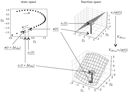
Figure 1 shows the correspondence between the state space and the function space . Although the observable function is the simple flat plane, the action of the Koopman operator yields the curved surface . The function gives the coordinate value after the time-evolution, i.e., .
Note that while it is possible to consider various types of observable functions, we focus only on the simple observables in the present work. A collection of the observable functions for the coordinates is called a full-state observable , which is a vector-valued observable function and
| (5) |
Again, we note that it is crucial to distinguish and .
2.3 Extended dynamic mode decomposition
As discussed in [23], we can obtain an approximate representation of the Koopman operator by a data-driven approach. That is, introducing a set of basis functions, called a dictionary, leads to a Koopman matrix for the time interval . The data-driven method is called the EDMD algorithm.
The EDMD algorithm requires a data set of snapshot pairs. The snapshot pairs are denoted as , where
| (6) |
and
| (7) | |||||
represents the number of snapshot pairs. The dictionary, , consists of basis functions, i.e.,
| (8) |
where for . For example, a dictionary with monomial functions for is given as
| (9) |
where the maximum degree of the monomial functions is , and means a scalar value . The dictionary spans a subspace .
Note that the dictionary with the monomial functions contains the full-state observable ; see the second and third elements on the right-hand side of (9). However, the action of the Koopman operator yields the function , which may not be in the spanned subspace . In this case, we have the following expansion:
| (10) |
where are the expansion coefficients. Similarly, we can consider the action for an arbitrary function , , and its coefficients . Note that the function before the time-evolution may not be in the spanned subspace , and the function is also approximately written as follows:
| (11) |
Since a linear combination of the dictionary functions yields an arbitrary function and its time-evolved function approximately, it is enough for us to consider the action of the Koopman operator to the dictionary. Then, the Koopman operator is approximated by a finite-size matrix as follows:
| (16) |
It is easy to determine the Koopman matrix from the dataset; we solve the following least squares problem numerically:
| (17) |
Note that a comparison with (10) and (17) immediately leads to the element at the -th row and the -th column of the Koopman matrix as follows:
| (18) |
Since the first dictionary function is time-invariant, for all .
In short, one can consider the linear action of in the function space instead of the nonlinear time-evolution on the state space, , in (2). This linearity naturally leads to the use of a linear combination of basis functions, which facilitates estimation from the data via the least squares method. The usage of linearity is one of the benefits of the Koopman operator approach.
2.4 Stochastic systems
As denoted in Sec. 1, the Koopman operator approach is also available for stochastic systems; for example, see [23, 32, 33]. In the stochastic cases, the action of the Koopman operator yields an expected value of a statistic for the state variable rather than the state variable itself. For example,
| (19) |
In the following, we briefly explain why the Koopman operator approach yields the expectation values from the viewpoint of the Fokker-Planck and the backward Kolmogorov equations.
Consider a -dimensional vector of stochastic variables, , and assume that the vector at time obeys the following stochastic differential equation:
| (20) |
where is a vector of drift coefficient functions, is a matrix of diffusion coefficient functions, and is a vector of Wiener processes . The Wiener processes satisfy
| (21) |
for . Let be the initial condition for the stochastic differential equation. The stochastic differential equation in (20) has a corresponding Fokker-Planck equation [34], which describes the time-evolution of the probability density function :
| (22) |
where
| (23) |
is the time-evolution operator for the Fokker-Planck equation. The initial condition at time is
| (24) |
where is the Dirac delta function.
Note that the time-evolved probability density function, , is formally written as
| (25) |
Then, the expectation for the observable function is given as follows:
| (26) |
where
| (27) |
and is the solution of the following partial differential equation, i.e., the so-called the backward Kolmogorov equation:
| (28) |
which leads to
| (29) |
Note that , and the initial condition is
| (30) |
Here, in (23) yields the time-evolution of the probability density function on the state space . By contrast, in (27) corresponds to the time-evolution of functions on the function space . In addition, (29) indicates that
| (31) |
and it is straightforwardly understandable that the Koopman operator yields the expectation after the time-evolution.
Note that the above discussion is also available to the deterministic cases. When there is no diffusion, i.e., , the time-evolution operator includes only the first-order derivatives. While the second-order derivatives lead to the effect of broadening the probability density function, the first-order derivatives correspond to the shift of the coordinates. Then, the zero diffusion cases retain the probability density function as the Dirac delta function; . Hence, the expectation yields the value of , and the previous discussions on the deterministic cases are recovered adequately.
3 Revisit on partial observations in deterministic systems
3.1 Use of time-dependent basis
Here, we follow [18] and revisit the effects of partial observations in deterministic systems. Note that the following discussions are slightly different from [18]. As discussed below, the absence of diffusion coefficients is crucial to connect the Koopman operator approach and the conventional discussions for partial observations, i.e., the Mori-Zwanzig formalism.
Assume that only some of the coordinates are observable, and we denote the index set as and the partial observables as whose elements are ; the number of partial observables is . For example, when we observe and in a case, , , and . We also introduce a dictionary that includes many basis functions related to the unobserved variables. We denote the number of dictionary functions as . The discussions on the function space and the introduction of the basis functions, i.e., the dictionary, lead to a linear algebraic approach for the nonlinear systems; this linearity is characteristic of the Koopman operator approach.
We discuss a case where the basis functions are time-dependent; this case corresponds to the discussion in [18]. In this case, an arbitrary function is expressed approximately as
| (32) |
Then, we derive an explicit representation of the time-evolution operator in (27). Using the same basis functions above, we approximate the operator as matrices; it is enough to consider the actions on and , and we have
| (33) |
and
| (34) |
Then, using the matrices, , , , and , the time-evolution equation is given as
| (41) |
As shown in [18], it is possible to derive the time-evolution equation for . First, we solve (41) for implicitly;
| (42) |
Then, inserting (42) to (41), we have
| (43) |
Replacing with and with , we have
| (44) |
where . is called the Markov transition matrix, which quantifies the interactions between the observables . is called the memory kernel and depends on the history of the observed quantity; (43) indicates that the memory effect stems from the path via the unobserved quantities. is referred to as noise since it depends on the initial values of the unobserved quantities . That is, there is no information about their explicit values, and then we cannot predict them.
3.2 Feature of deterministic systems
Note that (44) is an equation in the function space . It is crucial to distinguish the function space and the state space ; an element in is different from an element in the state vector in general. However, deterministic systems have a unique feature that one can interpret (44) as an equation for the state vector.
First, we focus on the time-evolution equation in (26); we see that the final expression yields the expectation values. Although the expectation value is not the state , the absence of the noise term does not change an initial Dirac-delta-type density function even in the time-evolution. That is,
| (45) |
Then, the expectation value is equal to the corresponding state;
| (46) |
This fact enables us to equate the observable function with the state .
Second, we introduce a different perspective on the time-evolution equation. In deterministic systems, , i.e., there is no noise. Hence, the second term on the right-hand side of (27) is absent. Then, the following operator yields the time-evolution in the function space:
| (47) |
When we consider the time-evolution for the observable function , the action of leads to
| (48) |
and then, we have
| (49) |
Note that (49) is the same form as the original time-evolution equation in the state space:
| (50) |
This fact also allows us to equate the time-evolution of in the function space with that of in the state space .
In short, although we should distinguish the function space and the state space, the feature of the deterministic system enables us to consider the derived equation (44) in the function space as the one in the state space. This feature justifies the coarse-grained approach based on the Mori-Zwanzig formalism; we can construct time-evolution equations of a smaller set of macroscopic variables that are measurable, and other unmeasured degrees of freedom play the role of noise.
4 Partial observations in stochastic systems
4.1 Discussion with time-independent basis functions
As discussed in Sec. 3, the derived equation in (44) is for the function space. Note that the function at time yields the expectation values in (26). Due to the presence of the noise term, even if the initial density function is the Dirac delta function, the values of and are different because the density function is spread out. Hence, the generalized Langevin equation in (44) is not directly related to the state vector .
Here, we discuss the generalized Langevin equation in the function space. Although the time-dependent basis in Sec. 3 is beneficial due to the connection with the state vector, it would be preferable to fix the basis functions in the discussion below. Then, we employ the following basis expansion:
| (51) |
where the expansion coefficients and are time-dependent, which differs from (32).
Then, we derive the time-evolution equation for the expansion coefficients and . In the derivation, we employ the bra and ket notations for the notational simplicity. Note that the notations are essentially the same as the Doi-Peliti method [35, 36, 37]; see the discussion in [38, 39, 40].
In the function space, we introduce the following ket states and :
| (52) | |||
| (53) |
where we omit the argument of functions, . By contrast, the bra states and are defined as follows:
| (54) | |||
| (55) |
where is a suitable measure to yield functions. From (52) and (54), we have the following orthonormal relation:
| (56) |
where is the Kronecker delta function.
It would be easy to explain with a concrete example. Hence, we here assume that there are only two observable variables, . Using the above bra and ket notations, (51) is rewritten as
| (57) |
The time-derivative of (57) leads to
| (58) |
Next, we take the action of on all terms from the left. Similar to the discussion in Sec. 3.1, we have the following time-evolution equation:
| (65) |
where we define
| (71) |
and
| (72) |
Although the matrix is not diagonal, the following assumption for the dictionary functions makes the discussion simple: the functions consist of monomial basis functions. Then, an element in has the following form:
| (73) |
where . The corresponding bra state is defined as
| (74) |
Then, we have the following orthogonal relation:
| (75) |
Note that the monomial functions for the observable states,
| (76) |
should not be included in . Using the above assumption for the dictionary functions, we have the following matrix in (71):
| (82) |
where we denote the diagonal part with . Since the matrix is diagonal, is also diagonal, which leads to
| (89) | |||||
| (94) |
Note that the multiplication of the diagonal matrix does not change the relationship between observable and unobserved functions. Since (94) has the same form as (41), we finally obtain the following equation similar to (44):
| (95) |
Although the form of (95) is similar to (41), there are differences. First, (95) is a vector-state equation for only one function . Second, the initial values of the coefficients are one-hot because we focus only on the observable functions . For example, assume that we focus on . Hence, we have the following equation for at the initial time :
| (96) |
which indicates that only the first element, , is 1, and the other terms become zero because the left-hand side is the function . Then, different from the time-dependent basis functions, the third term in the right-hand side in (95), i.e., the noise term, vanishes;
| (97) |
where and . Note that different from (44), it is not straightforwardly clear that the use of time-delayed states is beneficial. The second term on the right-hand side in (97) is related to the expansion coefficient, which does not directly correspond to the delayed state.
4.2 Effectiveness of delay embedding
As mentioned above, it is crucial to distinguish the state and function spaces. The discussions in Sec. 3.1 and Sec. 4.1 are based on the Koopman operator approach which focuses on the function space. The discussion in Sec. 3.2 focuses on the feature of the deterministic systems, which yields the connection with the state and function spaces.
It is well known that delay embedding is effective in deterministic systems [24, 25, 33, 41, 42]. The effectiveness of delay embedding could be understandable from the viewpoint of the Takens theorem [43]; see also the discussions in [18]. However, in stochastic systems, it is not straightforward to apply the discussion based on the Takens theorem because we consider the function space. Here, we discuss the effectiveness of the delay embedding in the stochastic systems.
As discussed in Sec. 2, the introduction of the dictionary enables us to deal with the nonlinearity within the Koopman operator approach. However, assuming the monomial basis functions, the use of higher-order basis functions causes the so-called curse of dimensionality, which exponentially increases the size of the dictionary. In the discussion in Sec. 4.1, the basis functions affect the second term on the right-hand sides in (95) and (97). The approximation by a finite dictionary can significantly reduce accuracy.
Here, note that the Koopman operator approach leads to
| (98) |
for an observable function . Then, we rewrite (98) formally as follows:
| (99) |
Since and include various functions, the exponential in (99) yields various basis functions not included in the finite dictionary. Hence, they are suitable for representing the subspace spanned by the time-evolution operator, and we could expect that the delay embedding will work well. In the next section, we will demonstrate the effectiveness of the delay embedding. Empirical insight into the characteristics of the noise effects will also be discussed.
5 Numerical experiments on the noise effects
5.1 Two examples
To investigate how stochasticity affects the partial observation, we perform numerical experiments. In [18], the data-driven approach enables us to obtain the Markov transition matrix and the memory kernel in (44) for the deterministic cases, and the relationship between the memory kernel and the delay embedding is describe. In the stochastic cases, as discussed above, it is not straightforward to connect the memory kernel in (97) with the delay embedding. Hence, we investigate the effects of the delay embedding with the data-driven approach based on the EDMD algorithm in Sec. 2.3.
For deterministic systems, it is common that there are many variables, and we observe only a few of them. For the stochastic systems here, we assume that the noise term includes most of the unobserved effects. As discussed below, it is necessary to consider higher-order dictionary functions to evaluate the higher-order statistics in stochastic systems, which leads to high computational costs. Hence, as demonstrations, we examine the following two examples and the effects of partial observation.
The first one is the van der Pol system [44] with additive noises:
| (100) | |||
| (101) |
The second one is the Lorentz system [45] with additive noises:
| (102) | |||
| (103) | |||
| (104) |
In all the numerical experiments, we assume that the noise amplitude for each variable is common: for the van der Pol system, and for the Lorentz system. The system parameters are set to for the van der Pol system, and , , and or for the Lorentz system; we tried two values for the parameter , as discussed below.
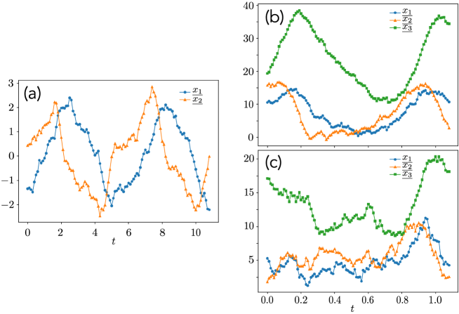
Figure 2 shows examples of sampled trajectories. The Euler-Maruyama approximation is employed [46]; for the van der Pol system, and for the Lorentz system. Figure 2 corresponds to the van der Pol system with the noise amplitude ; we see the noisy behavior along the limit cycle. Figures 2(b) and 2(c) correspond to the Lorentz system with noise amplitude . The difference with Figs. 2(b) and 2(c) is in the system parameter ; in Fig. 2(b) and in Fig. 2(c). Although the Monte Carlo simulations are performed with the small time interval , we construct the snapshot pairs from the generated data. Here, we set the time intervals as for the van der Pol system and for the Lorentz system. The markers in Fig. 2 are the observed data points.
5.2 Evaluation of approximate values of exact solutions
In deterministic systems, it is easy to obtain numerically exact solutions, which is necessary to discuss the accuracy of the partial observation. That is, the numerical time integration, such as the Runge-Kutta method, yields a good numerical approximation for the exact solutions. By contrast, the noise in the stochastic system prevents us from such numerical time integration. Although the Monte Carlo algorithm based on the Euler-Maruyama approximation is available for time integration, we should generate many sample trajectories to estimate the exact solutions for statistics. Since it is computationally impractical to obtain solutions with high accuracy using the Monte Carlo method, we directly derive the Koopman matrix for the stochastic system. The numerical procedure is essentially the same as [39, 40, 47]; we explain it briefly in the context of the present paper.
For example, consider three dimensional cases such as the Lorentz system. Then, we define the dictionary in Sec. 2.3 as follows:
| (105) |
Note that (94) leads to the expansion coefficients for the observable function . Hence, when we can observe all variables, i.e., , we have the following expansion:
| (106) |
where and are obtained via the time integration of (94) with . Next, we perform the time integration of (94) with , and so on. Here, note that the action of to yields ; this indicates that the linear combination in (106) is directly related to the Koopman matrix . That is, the elements in the second row of the Koopman matrix correspond to the expansion coefficients and . The third and fourth rows are for and , respectively. Repeating this procedure, it is possible to evaluate the Koopman matrix numerically.
Here, we employ the Crank-Nicolson method to solve (94); the discrete time intervals for numerical time integration is set to for the van der Pol system and for the Lorentz system, respectively. As denoted above, we set the observation time interval for the snapshot pairs as for the van der Pol system and for the Lorentz system. The maximum degrees in the dictionary are for the van der Pol system and for the Lorentz system.
If there is no noise, we can compare the numerical results obtained by the evaluated Koopman matrix with those from the conventional numerical time integration based on the fourth-order Runge-Kutta method. For randomly selected initial coordinates ( for the van der Pol system and for the Lorentz system), the mean absolute errors for data points are less than . From these results, we confirmed that the finite dictionaries with the specified maximum degrees yield sufficient accuracy. Hence, we employ the evaluated Koopman matrix from (94) as true solutions.
5.3 Settings for the EDMD algorithm for partial observation
To investigate the effects of the partial observation, we employ the EDMD algorithm with the delay embedding. The EDMD algorithm is data-driven, and we generate the dataset as follows:
-
1.
Generate randomly initial coordinates. (For the van der Pol system, a uniform density with was used. For the Lorentz system, we used a uniform density with .)
-
2.
Using the Euler-Maruyama approximation, the time integration is simulated via the Monte Carlo method. The time intervals for time-evolution and observation are the same as those in Sec. 5.1.
-
3.
After relaxation time, we take data points, where is the maximum number of the delay embedding.
-
4.
The above procedure is repeated times.
We prepare snapshot pairs and construct the Koopman matrix from the dataset. Although data points for all coordinates are generated, we consider the partial observation with only one variable.
We should note the dictionary in the EDMD algorithm. In deterministic systems, it is common to use a naive delay embedding of the past coordinate, such as . Although this setting is enough to evaluate only the coordinate values, we should employ higher-order basis functions to evaluate higher-order statistics. That is, in the stochastic systems, and the evaluation of requires the monomial functions whose maximum degree is at least two.
To consider the higher-order basis functions with the delay embedding, we rewrite the variables in Sec. 2 with . When we observe the -th variable, we set
| (115) |
where is the number of the delay embedding. Then, we introduce higher-order monomial basis functions for to evaluate higher-order statistics. Since we will focus on the mean values and the variances, the maximum degree of the dictionary functions for is set as two, which leads to the following dictionary :
| (116) |
where is a function which yields the coordinate value in the past:
| (117) |
5.4 Comparison with higher-order dictionary functions and delay embedding
As discussed in Sec. 4.2, the delay embedding would improve the accuracy of statistics in the Koopman operator approach. Here, we present the numerical results for the van der Pol system with the noise amplitude .
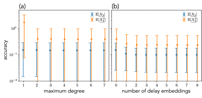
Figure 3 shows the accuracy in the partial observation setting. Here, only the second variable, , is measurable. In Fig. 3(a), we do not use the delay embeddings and the maximum degree of the basis functions is changed. We see that the sudden change occurs when the maximum degree is varied from 1 to 2; this fact means that the monomial functions with degree 2 are necessary to evaluate the second-order statistics.
Figure 3(b) shows the dependence of the number of delay embeddings and accuracy. Note that the dictionary introduced in Sec. 5.3 estimates adequately. From the numerical results, the increase in the number of embeddings improves the accuracy. We also see that there is a certain saturation point.
Compared with Figs. 3(a) and 3(b), we confirmed that the delay embedding is more effective than the usage of higher-order dictionary functions; this fact is common in all the other cases with other noise amplitude and the Lorentz system. Hence, the discussion in Sec. 4.2 would be valid; the delay embeddings are effective even in the partial observation cases in the stochastic systems.
5.5 Effects of higher order dictionary functions
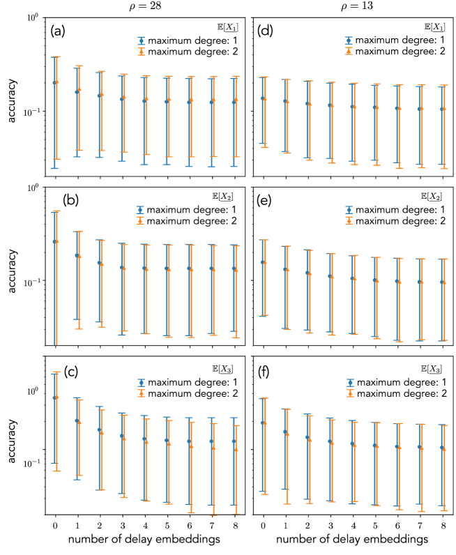
As explained in Sec. 4.2, the use of the higher-order basis functions is necessary for the evaluation of higher-order statistics. We here investigate its effects on the first-order statistics, i.e., the mean values. In the numerical experiments, we show the results for the Lorentz system; the same behavior was observed for the van der Pol system. The noise amplitude for the Lorentz system is set to .
Figure 4 shows the accuracy of the first-order statistics in the partial observation settings. We compare two dictionaries for the delay embeddings; one is the second-order monomial basis functions for in (116). The other one is the first-order monomial basis functions. Only in the case of , as shown in Fig. 4(c), there is a slight variation in accuracy for different dictionaries. The reason for this would be as follows. In the Lorentz system, differs from and ; (102) does not include a term related to , while each of the three equations includes and . Hence, the subspace spanned by the delay embedding with would be smaller than those with and . Then, the difference in the dictionary affects the partial observation of . As becomes smaller, the effects of noise through could be smaller. Hence, the effects on partial observations also become smaller; compared to Fig. 4(c), the difference in accuracy between different dictionaries in Fig. 4(f) is smaller. From these results, we conclude that the first-order basis functions with delay embeddings contain enough information for the time-evolution in the function space. The discussion in Sec. 4.2 justifies the results; the simple delayed function contains the information of the time-evolution; see (99).
Of course, note that the evaluation of the second-order statistics, such as , requires the second-order monomial basis functions.
5.6 Power-law behavior for the change of noise amplitude
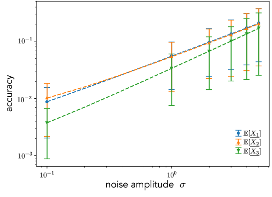
In general, external parameters, such as temperature, control the amplitude of the additive noise. Here, we investigate the effects of the noise amplitude. As a consequence, we found a power-law dependency of the accuracy with the noise amplitude.
Figure 5 depicts the dependency of the accuracy on the noise amplitude in the Lorentz system. Here, the plotted markers correspond to the accuracy for the delay embeddings with ; for all cases, the accuracy seems to have stopped declining in Fig. 4. We judged that the cases yield enough accurate estimation within the finite dictionary functions.
Note that we here employ the log-log plots in Fig. 5. From the plotted results, we assume the function form of the accuracy for the noise amplitude as follows:
| (118) |
Note that even in the noiseless cases, i.e., deterministic systems, there is a difference between the true statistics and the estimated ones because of the partial observation. Hence, we introduced in (118). The fitted results are also shown in Fig. 5; the fitting seems to be good.
| for | for | for | |
|---|---|---|---|
| 0.808 0.012 | 0.849 0.022 | 1.007 0.013 | |
| 0.773 0.036 | 0.661 0.024 | 0.820 0.022 |
In Table 1, we summarized the power-law exponent in (118) for the Lorentz system. Here, we repeated the same procedure for Fig. 5 five times and evaluated the means and standard deviations for the exponent . Although it is difficult to capture the meaning of the exponent , the exponent would reflect the effect of the unobserved part of the partial observation. The reason is as follows:
-
•
Although the EDMD algorithm can adequately deal with noise effects, partial observation causes a decrease in accuracy due to noise effects. The decrease occurs if the noise effects are orthogonal to the spanned space by the observable functions.
-
•
As discussed in Sec. 5.5, is the most significantly affected by partial observations. Then, the exponent for is the largest in Table 1. Note that the values of accuracy for are the smallest in Fig. 5; the increase in the accuracy due to the partial observation is not directly related to the actual accuracy values.
-
•
For the case, all the exponents becomes small. The reason is that the term in (103) becomes smaller, and the effects of the partial observation are also smaller. In particular, the effects of noise in are reduced directly via the term , and is most significantly affected.
From the above discussion, we expect that the power-law form and its exponent reflect some parts of the effects of the partial observation. If the ignored term has a strong nonlinearity, the impact of the partial observation should be considerable. Then, we perform additional numerical experiments for the following modified van der Pol systems, in which we replace (101) with
| (119) |
where is a nonlinear function. In the original van der Pol system, . This is an odd function, and then, we consider two cases with and .
| for | for | |
|---|---|---|
| 0.489 0.027 | 0.596 0.017 | |
| 0.567 0.030 | 0.652 0.029 | |
| 0.794 0.012 | 1.197 0.102 |
Table 2 shows the numerical results. As expected from the above discussion, the stronger the nonlinearity, the larger the exponent.
6 Discussions
In this work, we focused on the partial observations in stochastic systems. The Koopman operator approach is also available, and it is crucial to note the difference between state variables and observable functions. In other words, the Koopman operator approach gives an expected value, not the value of the state variable. The deterministic case is special, and the expected value coincides with the value of the state variable, i.e., . Although the stochasticity prevents us from using this simple connection, the delay embedding is effective even in stochastic systems. Note that there is a difference with the deterministic case, i.e., higher-order dictionary functions for the embedded states are necessary to evaluate higher-order statistics. In addition, the numerical experiments clarified that the noise dependency for accuracy exhibits a power-law behavior, and the exponent could reflect the characteristics of the partial observations.
There are some remaining tasks. First, it is not clear why the dependency of accuracy on the noise amplitude exhibits the power-law form in (118). Second, one should investigate the theoretical connection between the exponent in the power-law form and the information loss in partial observations. While we performed several other numerical experiments, we have not yet found a quantitative correspondence.
As mentioned above, there has been little discussion of partial observations in stochastic systems. Modeling based on stochastic differential equations is popular. Hence, further studies on partial observations are desirable from a practical standpoint. We believe that this study will serve as a starting point for future research.
References
References
- [1] Zwanzig R 1961 Phys. Rev. 124 983
- [2] Mori H 1965 Prog. Theor. Phys. 33 423
- [3] Zwanzig R 1973 J. Stat. Phys. 9 215
- [4] Chorin A J, Hald O H and Kupferman R 2000 Proc. Nat. Acad. Sci. 97 2968
- [5] Chorin A J, Hald O H and Kupferman R 2002 Physica D 166 239
- [6] Chorin A J and Stinis P 2006 Comm. Appl. Math. Comp. Sci. 1 1
- [7] Gouasmi A, Parish E J and Duraisamy K 2017 Proc. R. Soc. A 473 20170385
- [8] te Vrugt M, Topp L, Wittkowski R and Heuer A 2024 J. Chem. Phys. 161 094904
- [9] Netz R R 2024 Phys. Rev. E 110 014123
- [10] Chorin A J and Lu F 2015 Proc. Nat. Acad. Sci. 112 9804
- [11] Meyer H, Pelagejcev P and Schilling T 2019 Europhys. Lett. 128 40001
- [12] Maeyama S and Watanabe T H 2020 J. Phys. Soc. Jpn. 89 024401
- [13] González D, Chinesta F and Cueto E 2021 J. Comp. Phys. 428 109982
- [14] Tian Y, Lin Y T, Anghel M and Livescu D 2021 Phys. Fluids 33 125118
- [15] Venturi D and Li X 2023 Res. Math. Sci. 10 23
- [16] Gupta P, Schmid P, Sipp D, Sayadi T and Rigas G 2025 Proc. R. Soc. A 481 20240259
- [17] Lin K K and Lu F 2021 J. Comp. Phys. 424 109864
- [18] Lin Y T, Tian Y, Livescu D and Anghel M 2021 SIAM J. Appl. Dyn. Syst. 20 2558
- [19] Lin Y T, Tian Y, Perez D and Livescu D 2023 SIAM J. Appl. Dyn. Syst. 22 2890
- [20] Koopman B O 1931 Proc. Natl. Acad. Sci. 17 315
- [21] Rowley C W, Mezić I, Bagheri S, Schlatter P and Henningson D S 2009 J. Fluid Mech. 641 115
- [22] Schmid P J 2010 J. Fluid Mech. 656 5
- [23] Williams M O, Kevrekidis I G and Rowley C W 2015 J. Nonlinear Sci. 25 1307
- [24] Arbabi H and Mezić I 2017 SIAM J. Appl. Dyn. Syst. 16 2096
- [25] Brunton S L, Brunton B W, Proctor J L, Kaiser E and Kutz J N 2017 Nature Comm. 8 19
- [26] Mauroy A, Susuki Y and Mezić I 2020 The Koopman Operator in Systems and Control: Concepts, Methodologies, and Applications, ed Mauroy A, Mezić I and Susuki Y (Cham: Springer)
- [27] Budišić M, Mohr R and Mezić I 2012 Chaos 22 596
- [28] Mezić I 2013 Annu. Rev. Fluid Mech. 45 357
- [29] Rowley C W and Dawson S T M 2017 Annu. Rev. Fluid Mech. 49 387
- [30] Mezić I 2021 Notices of Amer. Math. Soc. 68 1087
- [31] Brunton S L, Budisǐć M, Kaiser E and Kutz J N 2022 SIAM Rev. 64 229
- [32] Črnjarić-Žic N, Maćešić S and Mezić I 2020 J. Nonlinear Sci. 30 2007
- [33] Wanner M and Mezić I 2022 SIAM J. Appl. Dyn. Syst. 21 1930
- [34] Gardiner C 2009 Stochastic methods: A handbook for the natural and social sciences, 4th edition (Berlin Heidelberg: Springer)
- [35] Doi M 1976 J. Phys. A: Math. Gen. 9 1465
- [36] Doi M 1976 J. Phys. A: Math. Gen. 9 1479
- [37] Peliti L 1985 J. Physique 46 1469
- [38] Ohkubo J 2013 J. Phys. A: Math. Theor. 46 375004
- [39] Ohkubo J and Arai Y 2019 J. Stat. Mech. 063202
- [40] Takahashi S and Ohkubo J 2023 J. Stat. Phys. 190 159
- [41] Clainche S L and Vega J M 2017 SIAM J. Appl. Dyn. Syst. 16 882
- [42] Kamb M, Kaiser E, Brunton S L and Kutz J N 2020 SIAM J. Appl. Dyn. Syst. 19 886
- [43] Takens F 1981 Lect. Notes in Math. 898 366
- [44] Van der Pol B 1926 The London, Edinburgh and Dublin Phil. Mag. & J. of Sci. 2, 978
- [45] Lorenz E N 1963 J. Atmos. Sci. 20 130
- [46] Kloeden P E and Platen E 1992 Numerical Solution of Stochastic Differential Equations (Berlin: Springer)
- [47] Ohkubo J 2021 J. Stat. Mech. 2021 013401