Labeling Multipath via Reconfigurable Intelligent Surface

First, we express (6) as a formulation of (1) as

where

We note from (7) that ${\bf h}^{[0]}$ is fixed while ${\bf h}^{[k]}(t)$ is time variant due to the phase toggling by RISs over time slots. Therefore, we can leverage this property to sperate the RIS channels from the overall received signal.

Specifically, by subtracting the received signal vector by its first time slot $t=1$, we obtain

for $t=2,\ldots$, where $\Delta\alpha_{l,t}^{[k]}=\alpha_{l}^{[k]}(t)-\alpha_{l}^{[k]}(1)$ and $\Delta{\bf w}_{t}={\bf w}(t)-{\bf w}(1)$. Clearly, only the RIS channels (i.e., $k\neq 0$) remain in $\Delta{\bf y}_{t}$. We can set the phase shift to make $\alpha_{l}^{[k]}(t)=\alpha_{l}^{[k]}(1)$ for several specific RISs. In this manner, we obtain $\Delta\alpha_{l,t}^{[k]}=0$ and can further remove inter-RIS interferences from $\Delta{\bf y}_{t}$. According to the contains in $\Delta{\bf y}_{t}$, we classify the channel flipping mechanism into two modes as follows.

• •

  Multilabeling mode. In this mode, $\Delta{\bf y}_{t}$ comprises multiple RIS channels as in (10). This mode provides multiple diversities for RIS channels, but it complicates the subsequent parameter extraction procedure.

• •

  Single-labeling mode. In this mode, $\Delta{\bf y}_{t}$ only contains a single RIS channel. This mode can be realized by changing the surface phases of only one RIS at each time slot while other RISs keep the same phase. For ease of understanding, we take an example with two RISs and three time slots. In the first time slot, the two RISs set their initial surface phases. In the second time slot, RIS1 varies the surface phase while RIS2 keeps the same phase as in the first time slot. In the third time slot, RIS2 varies the surface phase while RIS1 keeps the same phase as the first time slot. Therefore, we can resolve RIS1 channel and RIS2 channel from $\Delta{\bf y}_{2}$ and $\Delta{\bf y}_{3}$, respectively.

The RIS channels in $\Delta{\bf y}_{t}$ are usually weak, while we can improve the channel quality by using the multiple snapshots of $\Delta{\bf y}_{t}$ to mitigate the noise effect. To extract the path parameters (i.e., delay, AoA, and complex gain) of the RIS channel, we apply multisnapshot Newtonized orthogonal matching pursuit (MNOMP) [11]. The NOMP-based method [12] exhibits better performance than other state-of-the-art algorithms with a lower complexity.

For ease of notation, we first consider the single-labeling mode and remove the superscript $[k]$ from (10). In this case, we rewrite (10) as

for $t\in{{\mathcal{T}}=\{2,\ldots,T\}}$, where $T$ is the number of snapshots. The problem of extracting 3-tuples of the paths $(\Delta{\boldsymbol{\alpha}},{\boldsymbol{\theta}},{\boldsymbol{\tau}})=(\{\Delta\alpha_{l,2},\ldots,\Delta\alpha_{l,T}\},\theta_{l},\tau_{l})$ can be written as the joint minimization problem

Optimization problem (12) involves high-dimensional jointly searching of $(\Delta{\boldsymbol{\alpha}},{\boldsymbol{\theta}},{\boldsymbol{\tau}})$, which is intractable. MNOMP uses a detection-estimation method to separate each path iteratively and solve (12) efficiently. MNOMP first identifies the strongest signal path, subtracts it from $\left\{\Delta{\bf y}_{t}\right\}_{t\in{\mathcal{T}}}$, and then determines the next strongest path using the residual signal. The procedure consists of two stages:

• 1)

  Coarse detection. Coarse estimations of AoA, ToA, and complex gain are obtained by precomputed ${\bf v}(\theta,\tau)$ as follows

  	$$(\hat{\theta},\hat{\tau})=\underset{\theta\in{\boldsymbol{\Theta}},\tau\in{\boldsymbol{\Gamma}}}{\rm argmax}\ \sum_{t=1}^{T}|{\bf v}^{H}(\theta,\tau)\Delta{\bf y}_{t}|,$$		(13a)
  	$$\Delta\hat{\alpha}_{t}={{\bf v}^{H}(\hat{\theta},\hat{\tau})\Delta{\bf y}_{t}}/{\|{\bf v}(\hat{\theta},\hat{\tau})\|_{2}^{2}},\ t\in{\mathcal{T}},$$		(13b)

  where ${\boldsymbol{\Theta}}$ and ${\boldsymbol{\Gamma}}$ are the discretized sets of AoAs and ToAs, respectively.

• 2)

  Refinement. Let

  $$J_{\rm r}(\Delta{\boldsymbol{\alpha}},\theta,\tau)=\sum_{t=2}^{T}\left\|\Delta{\bf y}_{t}-\Delta\alpha_{t}{\bf v}{\left(\theta,\tau\right)}\right\|_{2}^{2},$$

  (14)

  where $\Delta{\boldsymbol{\alpha}}=(\Delta\alpha_{2},\ldots,\Delta\alpha_{T})$. The estimations are refined using the Newton method:

  	$\displaystyle(\hat{\theta},\hat{\tau})$	$\displaystyle\leftarrow(\hat{\theta},\hat{\tau})-[\ddot{J_{\rm r}}(\hat{{\boldsymbol{\alpha}}},\hat{\theta},\hat{\tau})]^{-1}\dot{J_{\rm r}}(\hat{{\boldsymbol{\alpha}}},\hat{\theta},\hat{\tau}),$		(15a)
  	$\displaystyle\Delta\hat{\alpha}_{t}$	$\displaystyle\leftarrow{{\bf v}^{H}(\hat{\theta},\hat{\tau})\Delta{\bf y}_{t}}/{\|{\bf v}(\hat{\theta},\hat{\tau})\|_{2}^{2}},\ t\in{\mathcal{T}},$		(15b)

  where $\ddot{J_{\rm r}}(\cdot)$ and $\dot{J_{\rm r}}(\cdot)$ are the Hessian and gradient of $J_{\rm r}$ with respect to $(\theta,\tau)$ at the current estimation $(\hat{\theta},\hat{\tau})$ provided by (13a), respectively. For $t\in{\mathcal{T}}$, we subtract the detected path from $\Delta{\bf y}_{t}$ and obtain the corresponding residual signal $\Delta{\bf y}_{t}\leftarrow\Delta{\bf y}_{t}-\Delta\hat{\alpha}_{t}{\bf v}(\hat{\theta},\hat{\tau})$.

The two steps are repeated with the residual signal to estimate other paths. To improve accuracy, the refinement steps are repeated after each new detection for all the paths in a cyclic manner for a few rounds.

We notice that the complex coefficient $\hat{\alpha}_{t}$ contains the labeling information of a RIS, which enables us to associate the path with its labeling RIS. To make the idea explicitly, we unfold the complex coefficient of RIS ${\bf a}_{\rm RIS}^{T}{(\tilde{\theta}_{l}^{[k]})}{\rm diag}({\boldsymbol{\phi}}^{[k]}(t)){\bf a}_{\rm RIS}{(\psi_{l}^{[k]})}$ as

where $a_{m}(\cdot)$ denotes the array response of the $m$-th subsurface of RIS. If we fix the phases of all subsurfaces, said $\phi_{m}^{[k]}(t)=\phi^{[k]}(t)$ for $m=1,\ldots,M$, then (16) can be written as

where

By combining (17) and (2), we write (4) as

where we define $\beta_{l}^{[k]}=g_{l}^{[k]}a_{l}^{[k]}$ for ease of expression. Applying (19), we write

where $\Delta\gamma_{l,t}^{[k]}=\gamma_{l}^{[k]}(t)-\gamma_{l}^{[k]}(1)$. In (20), $\beta_{l}^{[k]}$ is the coefficient depending on the propagation attenuation and incidental/reflection angles, whereas $\Delta\gamma_{l,t}^{[k]}$ is the coefficient depending on the surface phases of the RIS.

For the single-labeling mode, the $t$-th snapshot for the $k$-th RIS reads

where $t$ belongs to certain time slots ${\cal T}_{k}$. After extracting path parameters by MNOMP, we obtain complex coefficients $\{\Delta\hat{\alpha}_{l,t}^{[k]}:l=1,\ldots,L^{[k]},t\in{\cal T}_{k}\}$. We can extract the propagation attenuation coefficient of the $k$-th RIS with multiple snapshots via

Then, the LoS parameter between the $k$-th RISs and the Rx can be determined by selecting the maximum gain of $\hat{\beta}_{l}^{[k]}$ from $l=1,\ldots,L^{[k]}$.

For the multilabeling mode, we also can obtain complex coefficients $\{\Delta\hat{\alpha}_{l,t}:l=1,\ldots,\sum_{k=1}^{K}L^{[k]},t\in{\mathcal{T}}\}$ by using MNOMP. The extracted complex coefficients are not associated with any RISs in this stage. We notice that if a path is belong to the $k$-th RIS, then

Therefore, we calculate $\Delta\hat{\alpha}_{l,t}/\Delta\hat{\alpha}_{l,t+1}$ and then use it to associate the RIS. We use multiple snapshots of phase difference $\{\Delta\hat{\alpha}_{l,t}/\Delta\hat{\alpha}_{l,t+1}\}_{t=2}^{T-1}$ to improve the identification reliable because a snapshot of phase difference is unreliable when noise interference exists.

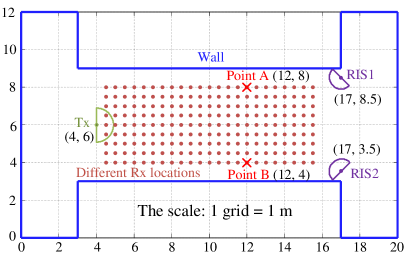
For the simulator, we consider an OFDM system following the 5G NR frame structure [13, ch. 5.4]. The system operates at $3.5$ GHz with $100$ MHz bandwidth and $2048$ subcarriers, where each subcarrier spaces $60$ kHz. The indoor layout is depicted in Fig. 1. We place the Tx and $2$ RISs in fixed locations while we vary the Rx locations. The transmission power of Tx is $1$ mW. Rx is equipped with a triangular antenna array, and the distance between the three antennas is half wavelength. Unlike the uniform linear array, which has ambiguity in the front and back directions, the triangular array used here can estimate AoA with $360^{\circ}$. The RIS is equipped with $M=10$ subsurfaces with fixed orientation, as shown in Fig. 1.

For Tx-to-Rx components, we consider one LoS and many NLoS paths, which are made up of one, double, and triple reflections from nearby walls [14, ch. 2]. For Tx-to-RIS-to-Rx components, we consider a direct path from the Tx to the RIS,¹¹1We also can consider reflection paths from the Tx to the RIS. and then the RIS scatters the incident signal from the Tx. The scattered signals reflect off multiple objects and become multiple paths arriving at the Rx. The paths from the RIS to the Rx also include one LoS and many one-to-triple reflections. The power of the propagation coefficient is modeled by $|g_{l}^{[k]}|=10^{P^{[k]}/20}\times 10^{P_{l}^{[k]}/20}$ [15], where the path losses of Tx-to-RIS $P^{[k]}$ and RIS-to-Rx $P_{l}^{[k]}$ are derived using the standard free-space propagation model. The RIS-to-Rx path considers the reflection path, where each has a different propagation distance, such that its path loss is indicated by the subscript “_l” to reflect this effect. In addition, we assume the addition of $5$ dB attenuation per reflection.

For the $t$-th time slot, the phase shift of RIS1 and RIS2 are denoted by $(\phi^{[1]}(t),\phi^{[2]}(t))$. The received signals adds white Gaussian noise at the level of $10^{-7}$, which results in the measured signal-to-noise ratio of $25$ dB at the central point $(10,6)$ in Fig. 1. To indicate the performance of multipath labeling, we use the mean absolute error (MAE) of AoA

where $\theta_{1}^{[k]}$ and $\hat{\theta}_{1}^{[k]}$ are the true and the estimated AoAs of the LoS path between the $k$-th RIS and the Rx. We obtain each subsequent result through the average of $1,000$ Monte Carlo trials.

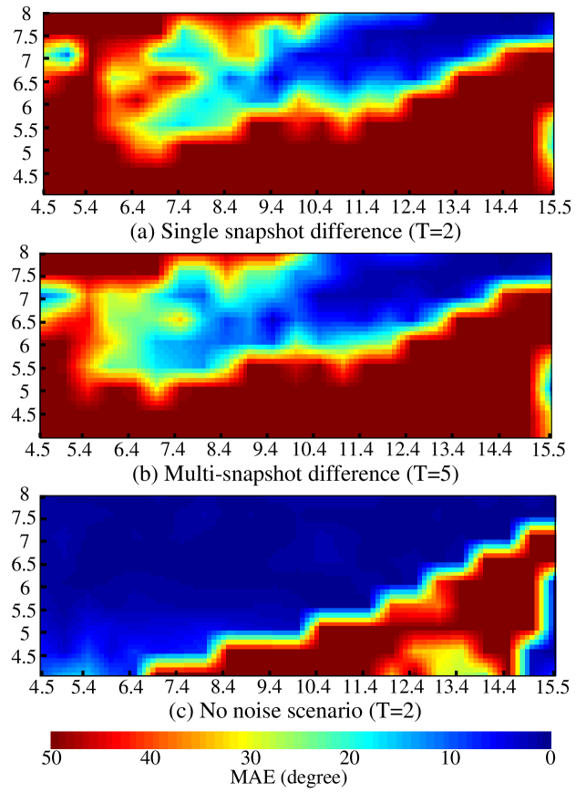
Fig. 4 shows the MAE of the AoA estimation for single-labeling mode under different number of snapshots. For $T=2$, we set ${(\phi^{[1]}(1),\phi^{[2]}(1))}=(0,0)$ and ${(\phi^{[1]}(2),\phi^{[2]}(2))}=(\pi,0)$. With this setting, we can separate the labeled multipath of RIS1 from others in $\Delta{\bf y}_{2}$. Fig. 4(a) illustrates the MAE with the single snapshot observation. The low MAE area (the blue area) is the location near RIS1. MAE degenerates when Rx is away from RIS1, so the shape of the blue area is related to the scattering energy of RIS1. Several areas are close to RIS1 but have large MAE because the area suffers from serious multipath interference resulting from the RIS scattering. In this situation, the LoS of RIS1 is difficult to be detected.

To understand the influence of noise and multipath interference, we provide examples of multisnapshot and no-noise scenarios, respectively. For the multisnapshot scenario, we set $(\phi^{[1]}(1),\phi^{[2]}(1))=(0,0)$ and $(\phi^{[1]}(t),\phi^{[2]}(t))=(\pi,0)$, $t=2,3,4,5$. Fig. 4(b) illustrates the corresponding MAE results. The low MAE area is larger than that in Fig. 4(a), indicating the substantial improvement in AoA accuracy due to the noise reduction by multiple snapshots. If the observation time slots can be sufficiently long, the noise effect can be completely removed while the multipath effect still exists. Fig. 4(c) illustrates the corresponding MAE results under no noise scenario with a single snapshot. The red area then illustrates the area that suffers from multipath interference.

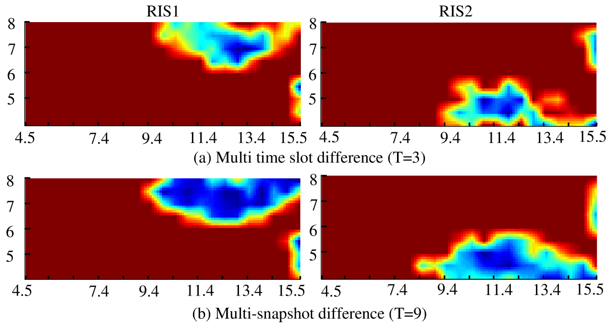
Fig. 4 show the MAE of AoA estimation for the multilabeling mode under different numbers of snapshots. For $T=3$, we set $(\phi^{[1]}(1),\phi^{[2]}(1))=(0,0)$, $(\phi^{[1]}(2),\phi^{[2]}(2))=(2\pi/3,4\pi/3)$, and $(\phi_{1}(3),\phi_{2}(3))=(4\pi/3,8\pi/3)$. Through path extraction and association, we can directly estimate the AoA from RIS1 and RIS2. The corresponding MAE results are shown in Fig. 4(a). Compared with Fig. 4(a), the low MAE area (the blue area) is reduced due to the inter-RIS interference.

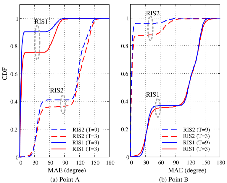
For multiple snapshots with ${T=9}$, we set $(\phi^{[1]}(1),\phi^{[2]}(1))=(0,0)$, $(\phi^{[1]}(2j),\phi^{[2]}(2j))=(2\pi/3,4\pi/3)$, $(\phi^{[1]}(2j+1),\phi^{[2]}(2j+1))=(4\pi/3,8\pi/3)$, $j=1,\ldots,4$. In Fig. 4(b), the low MAE area is larger than that in Fig. 4(a) because the noise effect can be largely reduced by the multisnapshot observations. We collect the MAE results from Points A and B of Fig. 1 and report a CDF plot for different snapshots in Fig. 4. In Point A, the performance of RIS1 is better than that of RIS2 because RIS1 is close to Point A. Similarly, the performance of RIS2 is better than that of RIS1 in Point B. At Points A or B, the performance of $T=9$ is better than $T=3$. In Fig. 4(a), MAE of $90\%$ is less than $10^{\circ}$ for RIS1 of $T=9$, and MAE of $70\%$ is less than $10^{\circ}$ for RIS1 of $T=3$. In Fig. 4(b), MAE of $95\%$ is less than $10^{\circ}$ for RIS2 of $T=9$, and MAE of $85\%$ is less than $10^{\circ}$ for RIS2 of $T=3$. The channel gain of RIS2 at Point B is larger than RIS1 at Point A. Thus, the performance of RIS2 at Point B is better than that of RIS1 at Point A.

The above results show that the noise effect on multipath labeling can be mitigated by long snapshots. However, long snapshots cannot solve the multipath and the inter-RIS interference effects. Therefore, we suggest using the single-labeling mode to remove the inter-RIS interference.

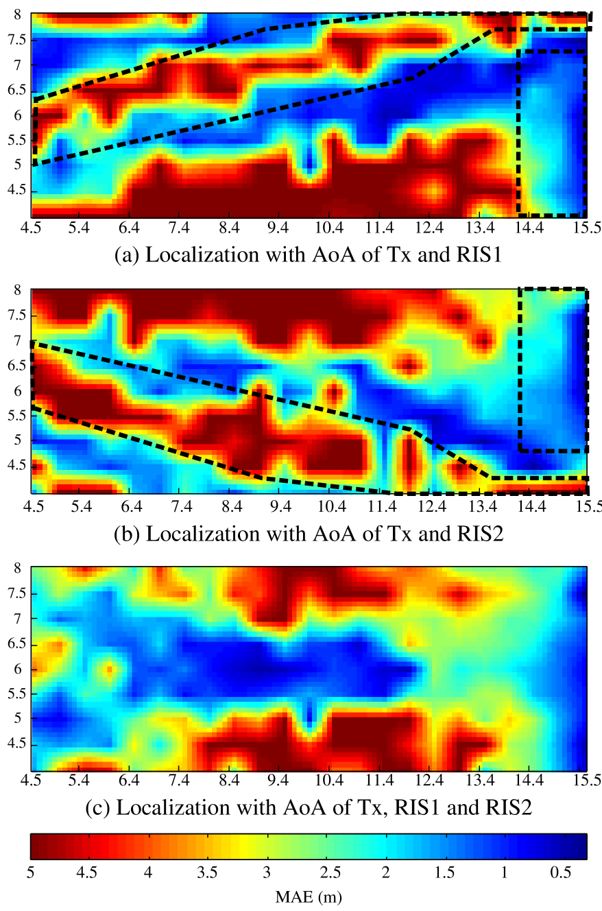
As an application, we consider the localization of Rx by using the estimated AoAs. We assume that the positions of Tx and RISs are known. Then, the Rx localization can be estimated by the closest point among the AoA intersections for the direct paths of RIS-to-Rx and Tx-to-Rx. The environment is the same as Fig. 1. We use the single-labeling mode with multiple snapshots with $T=9$. In this mode, the AoA of RISs can be obtained without inter-RIS interferences. We use the MAE of Rx position to indicate the performance of the localization results. Figs. 6(a)-(c) show the corresponding results with RIS1, RIS2, and both assistances, respectively. Note that one Tx without RIS assistance cannot perform localization through AoA. Therefore, we only show the localization results with RIS assistance.

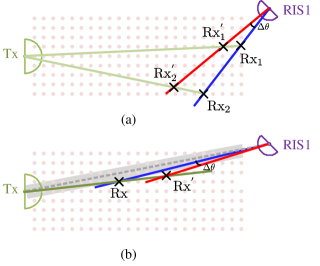
The low MAE area (the blue area) in Fig. 6(a) is similar to that in Fig. 4(b) except for 1) the right side area near RIS1 and 2) the direct line area between Tx and RIS1. The two exceptions reverse the results of Fig. 4(b). For example, the right side area near RIS1 of Fig. 4(b) is poor in AoA estimation while surprisingly good in localization in Fig. 6(a). To better understand the reasons for the two exceptions, we illustrate through the examples in Figs. 6(a) and 6(b), respectively. First, let us assume that the estimation quality of the AoA for the direct path of Tx-to-Rx is precise because the power of Tx is relatively large. Then, we consider that the AoA estimations from RIS1 have error $\Delta\theta$. With the error, the localizations of ${\rm Rx}_{1}$ and ${\rm Rx}_{2}$ are changed to ${\rm Rx}_{1}^{\prime}$ and ${\rm Rx}_{2}^{\prime}$, respectively. The two locations have quite different localization errors even they have the same AoA error. Clearly, the Rx located close to RIS1 has a smaller localization error than that far from RIS1. Next, we consider the reason for another exception. Fig. 6(b) illustrates that a small AoA error results in a significant localization error when Rx is on the direct line area between Tx and RIS1. The localization error is sensitive to the AoA error in the gray area, which results in poor localization results in Fig. 6(a). The same characteristics can be observed from Fig. 6(b), where RIS2 is used as the assistance. When RIS1 and RIS2 are used, Fig. 6(c) shows that multiple RISs extend the sensing area.

References

- [1] C. Huang et. al., “Reconfigurable intelligent surfaces for energy efficiency in wireless communication,” IEEE Trans. Wireless Commun., vol. 18, no. 8, Aug. 2019.
- [2] M. D. Renzo et al., “Smart radio environments empowered by reconfigurable ai meta-surfaces: An idea whose time has come,” EURASIP J. Wireless Commun. Netw., no. 129, pp. 1–20, May 2019.
- [3] S. Hu, F. Rusek, and O. Edfors, “Beyond massive MIMO: The potential of data transmission with large intelligent surfaces,” IEEE Trans. Signal Process., vol. 66, pp. 2746–2758, May 2018.
- [4] H. Wymeersch et al., “Radio localization and mapping with reconfigurable intelligent surfaces: Challenges, opportunities, and research directions,” IEEE Veh. Tech. Mag., vol. 15, no. 4, pp. 52–61, 2020.
- [5] M. Dunna, C. Zhang, D. Sievenpiper, and D. Bharadia, “ScatterMIMO: Enabling virtual MIMO with smart surfaces,” in Proc. in the 26th Annual Int. Conf. Mobile Computing and Netw., London, UK, 21–25 Sep. 2020, pp. 1–14.
- [6] J. He et al., “Large intelligent surface for positioning in millimeter wave MIMO systems,” in Proc. in IEEE 91st Veh. Tech. Conf., Antwerp, Belgium, 25–28 May 2020, pp. 1–5.
- [7] J. Zhang, Z. Zheng, Z. Fei, and X. Bao, “Positioning with dual reconfigurable intelligent surfaces in millimeter-wave MIMO systems,” in Proc. in IEEE/CIC Int. Conf. Commun. China (ICCC), Chongqing, China, 9–11 Aug. 2020, pp. 800–805.
- [8] H. Wymeersch and B. Denis, “Beyond 5G wireless localization with reconfigurable intelligent surfaces,” in Proc. in IEEE Int. Conf. Commun., Dublin, Ireland, 7–11 Jun. 2020, pp. 1–6.
- [9] B. Zheng and R. Zhang, “Intelligent reflecting surface-enhanced ofdm: Channel estimation and reflection optimization,” IEEE Wireless Communications Letters, vol. 9, no. 4, pp. 518–522, 2020.
- [10] S. Noh, H. Yu, and Y. Sung, “Training signal design for sparse channel estimation in intelligent reflecting surface-assisted millimeter-wave communication,” preprint, arXiv:2012.14221, 2020.
- [11] J. Zhu, L. Han, R. S. Blum, and Z. Xu, “Multi-snapshot newtonized orthogonal matching pursuit for line spectrum estimation with multiple measurement vectors,” Signal Process., vol. 165, pp. 175–185, Dec. 2019.
- [12] D. R. B. Mamandipoor and U. Madhow, “Newtonized orthogonal matching pursuit: Frequency estimation over the continuum,” IEEE Trans. Signal Process., vol. 64, no. 19, pp. 5066–5081, Oct. 2016.
- [13] E. Dahlman, S. Parkvall, and J. Skold, 5G NR: The Next Generation Wireless Access Technology. Academic Press, 2018.
- [14] A. Bergstrm, Timing-Based Localization using Multipath Information. Licentiate dissertation, Linkping University Electronic Press, Jan. 2020.
- [15] Ö. Özdogan, E. Björnson, and E. G. Larsson, “Intelligent reflecting surfaces: Physics, propagation, and pathloss modeling,” IEEE Wireless Communications Letters, vol. 9, no. 5, pp. 581–585, 2020.