Lagrangian acceleration in fully developed turbulence and its Eulerian decompositions

Before analyzing the DNS data, we present a brief theoretical analysis to obtain simplified relations between various Eulerian components of acceleration. For instance, it is straightforward to prove that in homogeneous turbulence, the correlation between an irrotational and a solenoidal vector is always zero (see Appendix). From this property, it follows that

	$\displaystyle\langle{\mathbf{a}}_{I}\cdot{\mathbf{a}}_{S}\rangle=0$		(3)
	$\displaystyle\langle{\mathbf{a}}_{I}\cdot{\mathbf{a}}_{L}\rangle=0.$		(4)

Additionally, using statistical stationarity, we can show (see Appendix) that

$\displaystyle\langle{\mathbf{a}}_{S}\cdot{\mathbf{a}}_{L}\rangle=0.$

(5)

Since ${\mathbf{a}}={\mathbf{a}}_{I}+{\mathbf{a}}_{S}$, it also follows from Eqs. (4) and (5) that

$\displaystyle\langle{\mathbf{a}}\cdot{\mathbf{a}}_{L}\rangle=0\ ,$

(6)

i.e., the Lagrangian acceleration $D{\mathbf{u}}/Dt$ is uncorrelated to the Eulerian acceleration $\partial u/\partial t$. This property directly yields the following result:

$\displaystyle\langle{\mathbf{a}}_{L}\cdot{\mathbf{a}}_{C}\rangle=-\langle|{\mathbf{a}}_{L}|^{2}\rangle.$

(7)

These relations allow us to write the acceleration variance as

	$\displaystyle\langle|{\mathbf{a}}|^{2}\rangle$	$\displaystyle=\langle|{\mathbf{a}}_{I}|^{2}\rangle+\langle|{\mathbf{a}}_{S}|^{2}\rangle$		(8)
	$\displaystyle\langle|{\mathbf{a}}|^{2}\rangle$	$\displaystyle=\langle|{\mathbf{a}}_{C}|^{2}\rangle-\langle|{\mathbf{a}}_{L}|^{2}\rangle.$		(9)

Thus, while the acceleration variance is given by the sum of variances of the pressure gradient and viscous terms, it is also obtained via a direct cancellation of convective and local components. We will now explore how the scaling of all these Eulerian contributions affect the scaling of acceleration variance itself.

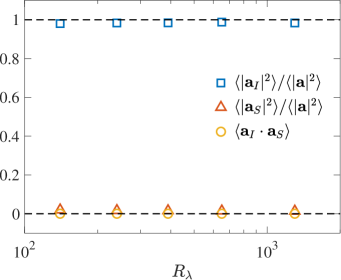
It is well known that acceleration variance is dominated by the irrotational pressure gradient contribution and the corresponding viscous contribution is negligible, i.e., $|{\mathbf{a}}_{I}|\gg|{\mathbf{a}}_{S}|$ Vedula and Yeung (1999); Tsinober et al. (2001). We first reaffirm this result in Fig. 1a which shows the fractional contributions of ${\mathbf{a}}_{I}$ and ${\mathbf{a}}_{S}$, and also the correlation $\langle{\mathbf{a}}_{I}\cdot{\mathbf{a}}_{S}\rangle$, which is zero as expected. It is evident that $\langle|{\mathbf{a}}|^{2}\rangle\approx\langle|{\mathbf{a}}_{I}|^{2}\rangle$. We can readily show that

$\displaystyle\langle{\mathbf{a}}\cdot{\mathbf{a}}_{I}\rangle=\langle{\mathbf{a}}_{C}\cdot{\mathbf{a}}_{I}\rangle=\langle|{\mathbf{a}}_{I}|^{2}\rangle\ ,\ \ \ \ \langle{\mathbf{a}}\cdot{\mathbf{a}}_{S}\rangle=\langle{\mathbf{a}}_{C}\cdot{\mathbf{a}}_{S}\rangle=\langle|{\mathbf{a}}_{S}|^{2}\rangle\ ,$

(10)

which demonstrate that both the pressure gradient and viscous contributions predominantly arise from the convective component. This is not surprising since we saw earlier that $\langle{\mathbf{a}}_{I}\cdot{\mathbf{a}}_{L}\rangle$ and $\langle{\mathbf{a}}_{S}\cdot{\mathbf{a}}_{L}\rangle$ are both zero. We shall further elaborate this point in the next subsection.

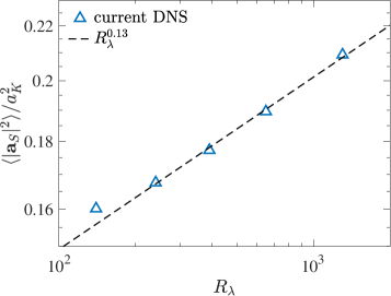
It is worth noting that, while the contribution from the viscous term ${\mathbf{a}}_{S}$ is negligible in comparison to ${\mathbf{a}}_{I}$, it is nevertheless finite and intimately connected to the fundamental dynamics of turbulence. In particular, its variance can be written as Monin and Yaglom (1975); Vedula and Yeung (1999)

$\displaystyle\langle|{\mathbf{a}}_{S}|^{2}\rangle/a_{K}^{2}=-\frac{35}{2}\frac{\mathcal{S}}{(15)^{3/2}}\ ,$

(11)

where $a_{K}=\langle\epsilon\rangle^{3/4}\nu^{-1/4}$ and $\mathcal{S}$ is the skewness of longitudinal velocity gradients, which is always negative in turbulence, characterizing the energy cascade from large to small scales Batchelor (1967); Frisch (1995). The skewness can also be related to vortex stretching Betchov (1956) and is known to weakly increase in magnitude as $R_{\lambda}^{0.13}$ Buaria et al. (2020c). This scaling matches the prediction from extending Eulerian multifractals to Lagrangian variables Sreenivasan and Meneveau (1988); Frisch (1995); Borgas (1993). Figure 1b shows a satisfactory agreement with this result (except at the lowest Reynolds number).

However, our recent work Buaria and Sreenivasan (2022a) computed the acceleration variance $\langle|{\mathbf{a}}_{I}|^{2}\rangle$ and found it to vary as $R_{\lambda}^{0.25}$. We expressed the acceleration analytically in terms of the fourth order velocity structure functions Hill and Wilczak (1995); Hill (2002), and showed that

$\displaystyle\langle|{\mathbf{a}}|^{2}\rangle/a_{K}^{2}\approx\langle|{\mathbf{a}}_{I}|^{2}\rangle/a_{K}^{2}\sim R_{\lambda}^{0.25}\ .$

(12)

The data from various sources, including our own DNS, show excellent agreement with this prediction (see Buaria and Sreenivasan (2022a); we also reaffirm it below). It then follows that an extension of Eulerian multifractals to explain intermittency of Lagrangian quantities is fraught with major uncertainties.

From Eq. (9), acceleration variance results from direct cancellation between the variances of ${\mathbf{a}}_{C}$ and ${\mathbf{a}}_{L}$. This cancellation is consistent with the random sweeping hypothesis proposed by Kraichnan Kraichnan (1964) – see also Tennekes Tennekes (1975) – which states that the small scales of turbulence are swept past an Eulerian observer on a much shorter time scale than the time scale governing their dynamical evolution. The nominal validity of this hypothesis is also implicitly reflected in the fact that ${\mathbf{a}}=D{\mathbf{u}}/Dt$ and ${\mathbf{a}}_{L}=\partial{\mathbf{u}}/\partial t$ are uncorrelated (see Eq. (6)).

The convective acceleration ${\mathbf{a}}_{C}={\mathbf{u}}\cdot\nabla{\mathbf{u}}$ essentially represents a correlation between the velocity and its gradients. Given the general understanding that the former characterizes the large scales and the latter the small scales, we can assume that the two are essentially uncorrelated (provided $R_{\lambda}$ is sufficiently high). Thus, simple scaling arguments suggest that $|{\mathbf{a}}_{C}|\sim u^{\prime}/\tau_{K}$ where $u^{\prime}$ is the root-mean-square (rms) velocity and $\tau_{K}$ is the Kolmogorov time scale, characterizing the rms of velocity gradients. We then have

$\displaystyle\langle|{\mathbf{a}}_{C}|^{2}\rangle/a_{K}^{2}=c\ R_{\lambda}\ ,$

(13)

where $c$ is some proportionality constant and we have utilized the classical estimate $u^{\prime}/u_{K}\sim R_{\lambda}^{1/2}$ Frisch (1995) ($u_{K}$ being the Kolmogorov velocity scale). To the first order, it can be also expected that $\langle|{\mathbf{a}}_{L}|^{2}\rangle$ also follows a similar scaling. This can be inferred indirectly by noting that

	$\displaystyle\langle|{\mathbf{a}}_{L}|^{2}\rangle$	$\displaystyle=\langle|{\mathbf{a}}_{C}|^{2}\rangle-\langle|{\mathbf{a}}|^{2}\rangle$		(14)
		$\displaystyle=\langle|{\mathbf{a}}_{C}|^{2}\rangle-\langle|{\mathbf{a}}_{I}|^{2}\rangle-\langle|{\mathbf{a}}_{S}|^{2}\rangle.$		(15)

where observations show that the scaling of $|{\mathbf{a}}_{C}|^{2}$ dominates over other two components.

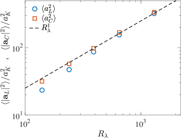
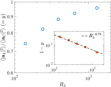
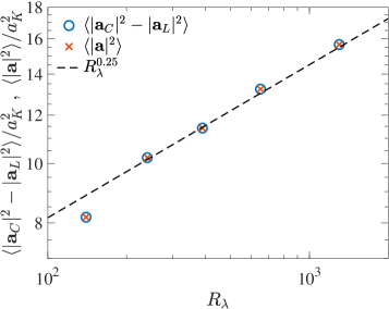
Figure 2a shows the variances of local and convective acceleration. It can be immediately seen that $|{\mathbf{a}}_{C}|^{2}/a_{K}^{2}$ follows a simple linear scaling in $R_{\lambda}$, as anticipated in Eq. (13). On the other hand, $|{\mathbf{a}}_{L}|^{2}/a_{K}^{2}$ approaches this scaling as ${R_{\lambda}}$ increases, but noticeably deviates at low ${R_{\lambda}}$. Using the results in Eqs. (11)-(15), the precise scaling of $\langle|{\mathbf{a}}_{L}|^{2}\rangle$ can be quantified as

$\displaystyle\langle|{\mathbf{a}}_{L}|^{2}\rangle/a_{K}^{2}=cR_{\lambda}-c_{1}R_{\lambda}^{0.25}-c_{2}R_{\lambda}^{0.13}\ ,$

(16)

where $c_{1}$ and $c_{2}$ are proportionality constants. Evidently, the deviations at lower ${R_{\lambda}}$ can be understood in terms of these additional terms. It also follows from here that the ratio $\langle|{\mathbf{a}}_{L}|^{2}\rangle/\langle|{\mathbf{a}}_{C}|^{2}\rangle$ has the form $1-(c_{1}/c)R_{\lambda}^{-0.75}-(c_{2}/c)R_{\lambda}^{-0.87}$. Asymptotically, when normalized by Kolmogorov variable, $\langle|{\mathbf{a}}|^{2}\rangle=\langle|{\mathbf{a}}_{C}|^{2}\rangle-\langle|{\mathbf{a}}_{L}|^{2}\rangle\approx c_{1}R_{\lambda}^{-0.25}$.

To verify the behaviors of ${\mathbf{a}}_{L}$ and ${\mathbf{a}}_{C}$ we plot in Fig. 2b the ratio $y=\langle|{\mathbf{a}}_{L}|^{2}\rangle/\langle|{\mathbf{a}}_{C}|^{2}\rangle$ as a function of ${R_{\lambda}}$. The inset shows $1-y$, which is in excellent agreement with a power law $R_{\lambda}^{-0.75}$. The ratio steadily approaches unity, which demonstrates that, asymptotically, only the $R_{\lambda}^{0.25}$ term contributes to Lagrangian acceleration. This is also confirmed by Fig. 2c, which shows $\langle|{\mathbf{a}}_{C}|^{2}\rangle-\langle|{\mathbf{a}}_{L}|^{2}\rangle$ normalized by Kolmogorov scales with the acceleration variance data from Buaria and Sreenivasan (2022a) – both sets of points are indistinguishable and in excellent agreement with $R_{\lambda}^{0.25}$ scaling.

The near cancellation between ${\mathbf{a}}_{L}$ and ${\mathbf{a}}_{C}$ can be further analyzed by noticing that ${\mathbf{a}}_{L}$ is solenoidal, whereas ${\mathbf{a}}_{C}$ is not; thus, they can never completely cancel each other. Further, since ${\mathbf{a}}_{I}$ is irrotational and ${\mathbf{a}}_{S}$ is solenoidal, we can write Tsinober et al. (2001)

	$\displaystyle{\mathbf{a}}_{C_{I}}$	$\displaystyle={\mathbf{a}}_{I}\ ,$		(17)
	$\displaystyle{\mathbf{a}}_{L}+{\mathbf{a}}_{C_{S}}$	$\displaystyle={\mathbf{a}}_{S}\ ,$		(18)

where we have decomposed ${\mathbf{a}}_{C}$ into irrotational and solenoidal components, i.e., ${\mathbf{a}}_{C}={\mathbf{a}}_{C_{I}}+{\mathbf{a}}_{C_{S}}$. Such a decomposition can readily be implemented in Fourier space using the Helmholtz decomposition, i.e., for a vector $\mathbf{V}$ with Fourier coefficient $\hat{\mathbf{V}}$, the Fourier coefficients of irrotational and solenoidal parts are, respectively, given as

$\displaystyle\hat{{\mathbf{V}}}_{I}({\mathbf{k}})=({\mathbf{k}}\cdot\hat{{\mathbf{V}}}){\mathbf{k}}/k^{2}\ ,\ \ \ \ \hat{{\mathbf{V}}}_{S}({\mathbf{k}})=\hat{{\mathbf{V}}}-\hat{{\mathbf{V}}}_{I}\ ,$

(19)

where ${\mathbf{k}}$ is the wave-vector and $k=|{\mathbf{k}}|$. Note that irrotationality is imposed in Fourier space by the condition ${\mathbf{k}}\times\hat{{\mathbf{V}}}_{I}=\mathbf{0}$, and solenoidality by ${\mathbf{k}}\cdot{\mathbf{V}}_{S}=0$ (both of which can be easily verified).

From the above decomposition, it trivially follows that $|{\mathbf{a}}_{C_{I}}|^{2}=|{\mathbf{a}}_{I}|^{2}$ and $\langle|{\mathbf{a}}_{C}|^{2}\rangle=\langle|{\mathbf{a}}_{C_{I}}|^{2}\rangle+\langle|{\mathbf{a}}_{C_{S}}|^{2}\rangle$ and we can also show that

	$\displaystyle\langle{\mathbf{a}}_{L}\cdot{\mathbf{a}}_{C_{S}}\rangle$	$\displaystyle=-\langle|{\mathbf{a}}_{L}|^{2}\rangle\ ,$		(20)
	$\displaystyle\langle|{\mathbf{a}}_{S}|^{2}\rangle$	$\displaystyle=\langle|{\mathbf{a}}_{C_{S}}|^{2}\rangle-\langle|{\mathbf{a}}_{L}|^{2}\rangle\ .$		(21)

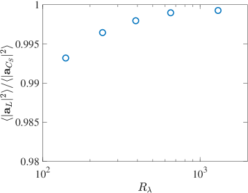
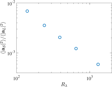
Thus, the very small solenoidal component ${\mathbf{a}}_{S}$ results from near perfect cancellation between ${\mathbf{a}}_{C_{S}}$ and ${\mathbf{a}}_{L}$. We quantify this in Fig. 3. Panel a shows that the ratio $\langle|a_{L}|^{2}\rangle/\langle|a_{C_{S}}|^{2}\rangle$ steadily approaches unity as ${R_{\lambda}}$ increases (though it cannot be strictly unity since $|{\mathbf{a}}_{S}|$ is always finite). In panel b, the ratio $\langle|a_{S}|^{2}\rangle/\langle|a_{L}|^{2}\rangle$ is shown, which steadily decreases with ${R_{\lambda}}$ as expected.

In summary, based on the present analysis, we can essentially write $|{\mathbf{a}}_{C}|\gtrsim|{\mathbf{a}}_{C_{S}}|\gtrsim|{\mathbf{a}}_{L}|\gg|{\mathbf{a}}|\approx|{\mathbf{a}}_{I}|=|{\mathbf{a}}_{C_{I}}|\gg|{\mathbf{a}}_{S}|$. Perhaps surprisingly, $\langle|{\mathbf{a}}|^{2}\rangle\approx\langle|{\mathbf{a}}_{I}|^{2}\rangle\sim R_{\lambda}^{0.25}$, while variances of the components ${\mathbf{a}}_{C}$ and ${\mathbf{a}}_{L}$ have far stronger dependencies on $R_{\lambda}$; for example, $\langle|{\mathbf{a}}_{C}|^{2}\rangle$ essentially scales as $R_{\lambda}$.

References

- La Porta et al. (2001) A. La Porta, G. A. Voth, A. M. Crawford, J. Alexander, and E. Bodenschatz, “Fluid particle accelerations in fully developed turbulence,” Nature 409, 1017–1019 (2001).
- Toschi and Bodenschatz (2009) F. Toschi and E. Bodenschatz, “Lagrangian properties of particles in turbulence,” Annu. Rev. Fluid Mech. 41, 375–404 (2009).
- Stelzenmuller et al. (2017) N. Stelzenmuller, J. I. Polanco, L. Vignal, I. Vinkovic, and N. Mordant, “Lagrangian acceleration statistics in a turbulent channel flow,” Phys. Rev. Fluids 2, 054602 (2017).
- Buaria et al. (2020a) D. Buaria, A. Pumir, F. Feraco, R. Marino, A. Pouquet, D. Rosenberg, and L. Primavera, “Single-particle Lagrangian statistics from direct numerical simulations of rotating-stratified turbulence,” Phys. Rev. Fluids 5, 064801 (2020a).
- Bec et al. (2006) J. Bec, L. Biferale, G. Boffetta, A. Celani, M. Cencini, A. Lanotte, S Musacchio, and F. Toschi, “Acceleration statistics of heavy particles in turbulence,” J. Fluid Mech. 550, 349–358 (2006).
- Sawford (1991) B. L. Sawford, “Reynolds number effects in Lagrangian stochastic models of turbulent dispersion,” Phys. Fluids A 3, 1577–1586 (1991).
- Wyngaard (1992) J. C. Wyngaard, “Atmospheric turbulence,” Annu. Rev. Fluid Mech. 24, 205–234 (1992).
- Pope (1994) S. B. Pope, “Lagrangian PDF methods for turbulent flows,” Annu. Rev. Fluid Mech. 26, 23–63 (1994).
- Wilson and Sawford (1996) J. D. Wilson and B. L. Sawford, “Review of Lagrangian stochastic models for trajectories in the turbulent atmosphere,” (1996).
- Kolmogorov (1941) A. N. Kolmogorov, “Local structure of turbulence in an incompressible fluid for very large Reynolds numbers,” Dokl. Akad. Nauk. SSSR 30, 299–303 (1941).
- Monin and Yaglom (1975) A. S. Monin and A. M. Yaglom, Statistical Fluid Mechanics, Vol. 2 (MIT Press, 1975).
- Yeung and Pope (1989) P. K. Yeung and S. B. Pope, “Lagrangian statistics from direct numerical simulations of isotropic turbulence,” J. Fluid Mech. 207, 531–586 (1989).
- Vedula and Yeung (1999) P. Vedula and P. K. Yeung, “Similarity scaling of acceleration and pressure statistics in numerical simulations of isotropic turbulence,” Phys Fluids 11, 1208–1220 (1999).
- Gotoh and Rogallo (1999) T. Gotoh and R. S. Rogallo, “Intermittency and scaling of pressure at small scales in forced isotropic turbulence,” J. Fluid Mech. 396, 257–285 (1999).
- Voth et al. (2002) G. A. Voth, A. La Porta, A. M. Crawford, J. Alexander, and E. Bodenschatz, “Measurement of particle accelerations in fully developed turbulence,” J. Fluid Mech. 469, 121–160 (2002).
- Sawford et al. (2003) B. L. Sawford, P. K. Yeung, M. S. Borgas, P. Vedula, A. La Porta, A. M. Crawford, and E. Bodenschatz, “Conditional and unconditional acceleration statistics in turbulence,” Phys. Fluids 15, 3478–3489 (2003).
- Mordant et al. (2004) N. Mordant, E. Lévêque, and J.-F. Pinton, “Experimental and numerical study of the Lagrangian dynamics of high Reynolds turbulence,” New J. Phys. 6, 116 (2004).
- Gylfason et al. (2004) A. Gylfason, S. Ayyalasomayajula, and Z. Warhaft, “Intermittency, pressure and acceleration statistics from hot-wire measurements in wind-tunnel turbulence,” J. Fluid Mech. 501, 213–229 (2004).
- Yeung et al. (2006) P. K. Yeung, S. B. Pope, A. G. Lamorgese, and D. A. Donzis, “Acceleration and dissipation statistics of numerically simulated isotropic turbulence,” Physics of fluids 18, 065103 (2006).
- Ishihara et al. (2007) T. Ishihara, Y. Kaneda, M. Yokokawa, K. Itakura, and A. Uno, “Small-scale statistics in high resolution of numerically isotropic turbulence,” J. Fluid Mech. 592, 335–366 (2007).
- Buaria and Sreenivasan (2022a) D. Buaria and K. R. Sreenivasan, “Scaling of acceleration statistics in high Reynolds number turbulence,” Phys. Rev. Lett. 128, 234502 (2022a).
- Borgas (1993) M. S. Borgas, “The multifractal Lagrangian nature of turbulence,” Philos. Trans. R. Soc. A 342, 379–411 (1993).
- Biferale et al. (2004) L. Biferale, G. Boffetta, A. Celani, B. J. Devenish, A. Lanotte, and F. Toschi, “Multifractal statistics of Lagrangian velocity and acceleration in turbulence,” Phys. Rev. Lett. 93, 064502 (2004).
- Ishihara et al. (2009) T. Ishihara, T. Gotoh, and Y. Kaneda, “Study of high-Reynolds number isotropic turbulence by direct numerical simulations,” Ann. Rev. Fluid Mech. 41, 165–80 (2009).
- Buaria et al. (2019) D. Buaria, A. Pumir, E. Bodenschatz, and P. K. Yeung, “Extreme velocity gradients in turbulent flows,” New J. Phys. 21, 043004 (2019).
- Rogallo (1981) R. S. Rogallo, “Numerical experiments in homogeneous turbulence,” NASA Technical Memo (1981).
- Buaria and Sreenivasan (2020) D. Buaria and K. R. Sreenivasan, “Dissipation range of the energy spectrum in high Reynolds number turbulence,” Phys. Rev. Fluids 5, 092601(R) (2020).
- Buaria et al. (2020b) D. Buaria, A. Pumir, and E. Bodenschatz, “Self-attenuation of extreme events in Navier-Stokes turbulence,” Nat. Commun. 11, 5852 (2020b).
- Buaria and Pumir (2021) D. Buaria and A. Pumir, “Nonlocal amplification of intense vorticity in turbulent flows,” Phys. Rev. Research 3, 042020 (2021).
- Buaria and Pumir (2022) D. Buaria and A. Pumir, “Vorticity-strain rate dynamics and the smallest scales of turbulence,” Phys. Rev. Lett. 128, 094501 (2022).
- Buaria et al. (2022) D. Buaria, A. Pumir, and E. Bodenschatz, “Generation of intense dissipation in high Reynolds number turbulence,” Philos. Trans. R. Soc. A 380, 20210088 (2022).
- Buaria and Sreenivasan (2022b) D. Buaria and K. R. Sreenivasan, “Intermittency of turbulent velocity and scalar fields using three-dimensional local averaging,” Phys. Rev. Fluids 7, L072601 (2022b).
- Buaria et al. (2015) D. Buaria, B. L. Sawford, and P. K. Yeung, “Characteristics of backward and forward two-particle relative dispersion in turbulence at different Reynolds numbers,” Phys. Fluids 27, 105101 (2015).
- Buaria et al. (2016) D. Buaria, P. K. Yeung, and B. L. Sawford, “A Lagrangian study of turbulent mixing: forward and backward dispersion of molecular trajectories in isotropic turbulence,” J. Fluid Mech. 799, 352–382 (2016).
- Buaria and Yeung (2017) D. Buaria and P. K. Yeung, “A highly scalable particle tracking algorithm using partitioned global address space (PGAS) programming for extreme-scale turbulence simulations,” Comput. Phys. Commun. 221, 246 – 258 (2017).
- Tsinober et al. (2001) A. Tsinober, P. Vedula, and P. K. Yeung, “Random Taylor hypothesis and the behavior of local and convective accelerations in isotropic turbulence,” Phys. Fluids 13, 1974–1984 (2001).
- Batchelor (1967) G. K. Batchelor, An Introduction to Fluid Dynamics (Cambridge University Press, Cambridge, 1967).
- Frisch (1995) U. Frisch, Turbulence: The Legacy of Kolmogorov (Cambridge University Press, Cambridge, 1995).
- Betchov (1956) R. Betchov, “An inequality concerning the production of vorticity in isotropic turbulence,” J. Fluid Mech. 1, 497–504 (1956).
- Buaria et al. (2020c) D. Buaria, E. Bodenschatz, and A. Pumir, “Vortex stretching and enstrophy production in high Reynolds number turbulence,” Phys. Rev. Fluids 5, 104602 (2020c).
- Sreenivasan and Meneveau (1988) K. R. Sreenivasan and C. Meneveau, “Singularities of the equations of fluid motion,” Phys. Rev. A 38, 6287–6295 (1988).
- Hill and Wilczak (1995) R. J. Hill and J. M. Wilczak, “Pressure structure functions and spectra for locally isotropic turbulence,” J. Fluid Mech. 296, 247–269 (1995).
- Hill (2002) R. J. Hill, “Scaling of acceleration in locally isotropic turbulence,” J. Fluid Mech. 452, 361–370 (2002).
- Kraichnan (1964) R. H. Kraichnan, “Kolmogorov’s hypotheses and Eulerian turbulence theory,” Phys. Fluids 7, 1723–1734 (1964).
- Tennekes (1975) H. Tennekes, “Eulerian and Lagrangian time microscales in isotropic turbulence,” J. Fluid Mech. 67, 561–567 (1975).