1
Lale: Consistent Automated Machine Learning
Abstract.
Automated machine learning makes it easier for data scientists to develop pipelines by searching over possible choices for hyperparameters, algorithms, and even pipeline topologies. Unfortunately, the syntax for automated machine learning tools is inconsistent with manual machine learning, with each other, and with error checks. Furthermore, few tools support advanced features such as topology search or higher-order operators. This paper introduces Lale, a library of high-level Python interfaces that simplifies and unifies automated machine learning in a consistent way.
1. Introduction
Machine learning (ML) is widely used in various data science problems. There are many ML operators for data preprocessing (scaling, missing imputation, categorical encoding), feature extraction (principal component analysis, non-negative matrix factorization), and modeling (boosted trees, neural networks). A machine learning pipeline consists of one or more operators that take the input data through a series of transformations to finally generate predictions. Given the plethora of ML operators (for example, in the widely used scikit-learn library (Buitinck et al., 2013)), the task of finding a good ML pipeline for the data at hand (which involves not only selecting operators but also appropriately configuring their hyperparameters) can be tedious and time consuming if done manually. This has led to a wider adoption of automated machine learning (AutoML), with the development of novel algorithms (such as SMAC (Hutter et al., 2011), hyperopt (Bergstra et al., 2011), and subsequent recent work (Liu et al., 2020)), open source libraries (auto-sklearn (Feurer et al., 2015), hyperopt-sklearn (Komer et al., 2014; Bergstra et al., 2015), TPOT (Olson et al., 2016)), and even commercial tools.
Scikit-learn provides a consistent programming model for manual ML (Buitinck et al., 2013), and various other tools (such as XGBoost (Chen and Guestrin, 2016), LightGBM (Ke et al., 2017), and Tensorflow’s tf.keras.wrappers.scikit_learn) maintain consistency with this model whenever appropriate. AutoML tools usually feature two pieces – (i) a way to define the search space corresponding to the pipeline topology, the operator choices in that topology, and their respective possible hyperparameter configurations, and (ii) an algorithm that explores this search space to optimize for predictive performance. Many of these also try to maintain consistency with the scikit-learn model but only when the user gives up all control and lets the tool completely automate the ML pipeline configuration, eschewing item (i) above. Users often want to retain some control over the automation, for example, to comply with domain-specific requirements by specifying operators or hyperparameter ranges to search over. While fine-grained control over the automation is possible (we will discuss examples), users need to manually configure the search space. This search space specification differs for each of the different AutoML tools and differs from the manual programming model.
We believe that proper abstractions are necessary to provide a consistent programming model across the entire spectrum of controlled automation. To this end, we introduce Lale, an open-source Python library111https://github.com/ibm/lale, built upon mathematically grounded abstractions of the elements of the pipeline (for example, topology, operator, hyperparameter configurations), and designed around scikit-learn (Buitinck et al., 2013) and JSON Schema (Pezoa et al., 2016). Lale provides a programming interface for specifying pipelines and search spaces in a consistent manner while providing fine-grained control across the automation spectrum. The abstractions also allow us to provide a consistent programming interface for capabilities for which no such interface currently exists: (i) search spaces with higher-order operators (operators, such as ensembling, that have other operators as hyperparameters), and (ii) search spaces that include search for the pipeline topology via context-free grammars (Chomsky, 1956). The contributions of this paper are:
-
1.
A pipeline specification syntax that is consistent across the automation spectrum and grounded in established technologies.
-
2.
Automatic search space generation from pipelines and schemas for a consistent experience across existing AutoML tools.
-
3.
Higher-order operators (for ensembles, batching, etc.) with automatic AutoML search space generation for nested pipelines.
-
4.
A grammar syntax for pipeline topology search that is a natural extension of the pipeline syntax.
Overall, we hope Lale will make data scientists more productive at finding pipelines that are consistent with their requirements and yield high predictive performance.
2. Problem Statement
Consistency is a core problem for AutoML and existing libraries fall short on this front. This section uses concrete examples from popular (Auto-)ML libraries to present four shortcomings in existing systems. We strive to do so in a factual and constructive way.
: Provide a consistent programming model across the automation spectrum.
There is a spectrum of AutoML ranging from manual machine learning (no automation) to hyperparameter tuning, operator selection, and pipeline topology search. Unfortunately, as users progress across this spectrum, the state-of-the-art libraries require them to learn and use different syntax and concepts.
Figure 2 shows an example from the no-automation end of the spectrum using scikit-learn (Buitinck et al., 2013). The code assembles a two-step pipeline of a PCA transformer and a LinearSVC classifier and manually sets their hyperparameters, for example, n_components=4.
The example in Figure 3 automates hyperparameter tuning and operator selection using GridSearchCV from scikit-learn. Lines 1–3 resemble Figure 2. Lines 4–11 specify a search space, consisting of a list of two dictionaries. In the first dictionary, Line 7 specifies the list of values to search over for the n_components hyperparameter of the PCA operator; Line 8 specifies the classify step of the pipeline to be a LinearSVC operator; and Line 9 specifies the list of values to search over for the C hyperparameter of the LinearSVC operator. The second dictionary is similar, but specifies the RandomForestClassifier.
The syntax for a pipeline (Figure 2 Lines 1–3) differs from that for a search space (Figure 3 Lines 4–11). The mental model is that operators and hyperparameters are pre-specified and then the search space selectively overwrites them with different choices. To do so, the code uses strings to name steps and hyperparameters, with a double underscore (’__’) name mangling convention to connect the two. Relying on strings for names can cause hard-to-detect mistakes (Baudart et al., 2019). In contrast, using a single syntax for both manual and automated pipelines would make them more consistent and would obviate the need for mangled strings to link between the two.
: Provide a consistent programming model across different AutoML tools.
Compared to GridSearchCV, Bayesian optimizers such as hyperopt-sklearn (Komer et al., 2014) and auto-sklearn (Feurer et al., 2015) speed up search using smarter search strategies. Unfortunately, each of these AutoML tools comes with its own syntax and concepts.
Figure 4 shows an example using the hyperopt-sklearn (Komer et al., 2014) wrapper for hyperopt (Bergstra et al., 2011). Line 1 specifies a discrete search space N with a logarithmic prior, a range from 2..8, and a quantization to multiples of 1. Line 2 specifies a continuous search space C with a logarithmic prior and a range from 1..1000. Line 4 sets the transform step of the pipeline to pca with hyperparameter n_components=N. Lines 5–7 set the classify step to a choice between linear_svc and random_forest.
Figure 5 shows the same example using auto-sklearn (Feurer et al., 2015). While power users can use the ConfigurationSpace used by SMAC (Hutter et al., 2011) to adjust search spaces for individual hyperparameters, we elide this for brevity. Line 2 sets the preprocessor to ’pca’ and Line 3 sets the classifier to a choice of ’linear_svc’ or ’random_forest’.
The syntaxes for the three AutoML tools in Figures 3, 4, and 5 differ. There are three ways to refer to the same operator: PCA, pca(..), and ’pca’. There are three ways to specify an operator choice: a list of dictionaries, hp.choice, and a list of strings. The mental model varies from overwriting to nested configuration to string-based configuration. Users must learn new syntax and concepts for each tool and must rewrite code to switch tools. Moreover, as we consider more sophisticated pipelines (beyond the simple two-step one presented in the example), the search space specifications get even more convoluted and diverse between these existing specification schemes. A unified syntax would make these tools more consistent, easier to learn, and easier to switch. Furthermore, this syntax should unify not just AutoML tools but also be consistent with the manual end of the spectrum (). More specifically, given that scikit-learn sets the de-facto standard for manual ML, the syntax should be scikit-learn compatible.
: Support topology search and higher-order operators in AutoML tools.
The tools previously discussed search operators and hyperparameters but do not optimize the topology of the pipeline itself. There are some tools that do, including TPOT (Olson et al., 2016), Recipe (de Sá et al., 2017), and AlphaD3M (Drori et al., 2019). Unfortunately, their methods for specifying the search space are inconsistent with manual machine learning and established tools. TPOT does not allow the user to specify the search space for pipeline topologies (the user can specify the set of operators and can fix the pipeline topology, disabling the topology search). Recipe and AlphaD3M use context-free grammars to specify the search space for the topology, but in a manner inconsistent with each other or with other levels of automation.
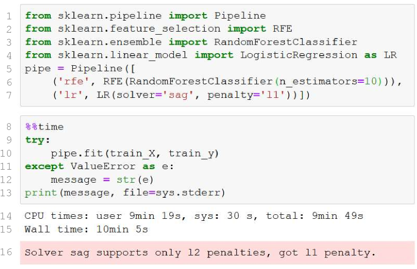
Some transformers (e.g. RFE in Figure 6 Line 7) and estimators (e.g. AdaBoostClassifier) are higher-order: they take other operators as arguments. Using the AutoML tools discussed so far to search inside their nested operators is not straightforward. The aforementioned TPOT, Recipe, and AlphaD3M do not handle higher-order operators in their search for pipeline topology.
A unified syntax for topology search and higher-order operators that is a natural extension of the syntax for manual machine learning, algorithm selection, and hyperparameter tuning would make AutoML more expressive while keeping it consistent.
: Check for invalid configurations early and prune them out of search spaces.
Even if the search for each hyperparameter uses a valid range in isolation, their combination can violate side constraints. Worse, these errors may be detected late, wasting time.
Figure 6 shows a misconfigured pipeline: the hyperparameters for LR in Line 7 are valid in isolation but invalid in combination. Unfortunately, this is not detected when the pipeline is created on Line 7. Instead, when Line 10 tries to fit the pipeline, it first fits the first step of the pipeline (see RFE in Line 6). Only then does it try to fit the LR and detect the mistake. This wastes 10 minutes (Line 15).
In contrast, a declarative specification of the side constraints would both speed up this manual example and enable AutoML search space generators to prune cases that violate constraints, thus speeding up the automated case too. Furthermore, in some situations, invalid configurations cause more harm than just wasted time, leading optimizers astray (Section 6). It is possible (with varying levels of difficulty) to incorporate these side constraints with the search space specification schemes used by the tools discussed earlier, but they each have inconsistent methods for doing this. Moreover, the complexity of these specifications make them error prone. Additionally, while these side constraints help the optimizer, they do not directly help detect misconfigurations (as in Figure 6). Custom validators would need to be written for each tool.
3. Programming Abstractions
This section shows Lale’s abstractions for consistent AutoML, addressing the problem statements from Section 2.
3.1. Abstractions for Declarative AutoML
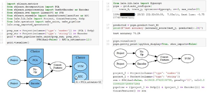
An individual operator is a data science algorithm (aka. a primitive or a model), which may be a transformer or an estimator such as classifier or a regressor. Individual operators are modular building blocks from libraries such as scikit-learn. Figure 1 Lines 2–6 contain several examples, e.g., import LinearSVC as SVM. Mathematically, Lale views an individual operator as a function of the form
This view uses currying: it views an operator as a sequence of functions each with a single argument and returning the next in the sequence. An individual operator (e.g., SVM) is a function from hyperparameters (e.g., dual=False) to a function from training data (e.g., train_X, train_y) to a function from input data (e.g., test_X) to output data (e.g., predicted in Figure 1 Line 17). In the beginning, all arguments are latent, and each step in the sequence captures the next argument as given. The scikit-learn terminology for the three curried sub-functions is init, fit, and predict. Viewing operators as mathematical functions avoids complications arising from in-place mutation. It lets us conceptualize bindings as lifecycle: each bound, or captured, argument unlocks the functionality of the next state in the lifecycle.
A pipeline is a directed acyclic graph (DAG) of operators and a pipeline is itself also an operator. Since a pipeline contains operators and is an operator, it is highly composable. Furthermore, viewing both individual operators and pipelines as special cases of operators makes the concepts more consistent. An example is make_pipeline(make_union(PCA, RFC), SVM), which is equivalent to ((PCA & RFC) >> ConcatFeatures >> SVM). Here, & is the and combinator and >> is the pipe combinator. Combinators make edges more explicit and code more concise. An expression x & y composes x and y without introducing additional edges. An expression x >> y introduces edges from all sinks of subgraph x to all sources of y. Mathematically, Lale views a pipeline as a function of the form
This uses currying just like individual operators, plus an additional at the start to capture the steps and edges. A pipeline is trainable if both and are given, i.e., the hyperparameters of all steps have been captured. To fit a trainable pipeline, iterate over the steps in a topological order induced by the edges. For each step , let be the training data for the step, which is either the pipeline’s training data if is a source or the predecessors’ output data otherwise. Then, recalling that is a curried function, calculate and . The trained pipeline substitutes trained steps for trainable steps in . To make predictions with a trained pipeline, simply interpret >> as function composition .
An operator choice is an exclusive disjunction of operators and is itself also an operator. Operator choice specifies algorithm selection, and by being an operator, addresses problem from Section 2. An example is (SVM | RFC), where | is the or combinator. Mathematically, Lale views an operator choice as a function of the form
This again uses currying. Argument is the list of operators to choose from. The of an operator choice consists of an indicator for which of its steps is being chosen, along with the hyperparameters for that chosen step. Once is captured, the operator choice is equivalent to just the chosen step, as shown in the visualization after Figure 1 Line 20.
The combined schema of an operator specifies the valid values along with search guidance for its latent arguments. It addresses problem from Section 2, supporting automated search with a pruned search space and early error checking all from the same single source of truth. Consider the pipeline PCA >> (J48 | LR), where PCA and LR are the principal component analysis and logistic regression from scikit-learn and J48 is a decision tree with pruning from Weka (Hall et al., 2009). These operators have many hyperparameters and constraints and Lale handles all of them. For didactic purposes, this section discusses only a representative subset. Figure 7 shows the JSON Schema (Pezoa et al., 2016) specification of that subset. The open-source Lale library includes JSON schemas for many operators, some hand-written and others auto-generated (Baudart et al., 2020). The number of components for PCA is given by , which can be a continuous value in or the categorical value mle. The prior distribution helps AutoML tools search faster. J48 has a categorical hyperparameter to enable reduced error pruning and a continuous confidence threshold for pruning. Mathematically, we denote allOf as , anyOf as , and not as . Even though the valid values for are , search should only consider values . The constraint in Lines 16–19 encodes a conditional by using the equivalent . LR has two categorical hyperparameters (solver) and (penalty), with a constraint that solvers sag and lbfgs only support penalty l2, which we already encountered in Figure 6. Going forward, we will denote a JSON Schema object with properties as dict{} and a JSON Schema enum as . Eliding priors, this means Figure 7 becomes:
To auto-configure an operator means to automatically capture , which involves jointly selecting algorithms (for operator choices) and tuning hyperparameters (for individual operators). We saw examples for doing this with scikit-learn’s GridSearchCV (Buitinck et al., 2013), hyperopt-sklearn (Komer et al., 2014), and auto-sklearn (Feurer et al., 2015) in Figures 3, 4, and 5. Lale offers a single unified syntax shown in Figure 1 Lines 15–16 to address problem from Section 2. Mathematically, let op be either an individual operator or a pipeline or choice whose or are already captured. That means op has the form . Then returns a function of the form . Section 4 discusses how to implement auto_configure using schemas.
3.2. Abstractions for Controlled AutoML
AutoML users rarely want to completely surrender all decisions to the automation. Instead, users typically want to control certain decisions based on their problem statement and expertise. This section discusses how Lale supports such controlled AutoML.
The lifecycle state of an operator is the number of curried arguments it has already captured that determines the functionality it supports. To enable controlled AutoML, Lale pipelines can mix operators with different states. The visualizations in Figure 1 indicate lifecycle states via colors. A planned operator, shown in dark blue, has captured only or , but is still latent. Planned operators support auto_configure but not fit or predict. A trainable operator, shown in light blue, has also captured , leaving latent. Trainable operators support auto_configure and fit but not predict. A trained operator, shown in white, also captures . Trained operators support auto_configure, fit, and predict. Later states subsume the functionality of earlier states, enabling user control over where automation is applied. The state of a pipeline is the least upper bound of the states of its steps.
Partially captured hyperparameters of an individual operator treat some of its hyperparameters as given while keeping the remaining ones latent. Specifying some hyperparameters by hand lets users control and hand-prune the search space while still searching other hyperparameters automatically. For example, Figure 1 Line 12 shows partially captured hyperparameters for SVM and RFC. The visualization after Line 13 reflects this in a tooltip for RFC. And the pretty-printed code after Line 20 shows that automation respected the given dual hyperparameter of SVM while capturing the latent C, penalty, and tol. Individual operators with partially captured hyperparameters are trainable: fit uses defaults for latents.
Freezing an operator turns future auto_configure or fit operations into an identity. PCA(n_components=4).freeze_trainable() >> SVM freezes all hyperparameters of PCA (using defaults for its latents), so auto_configure on this pipeline tunes only the hyperparameters of SVM. Similarly, on a trained operator, freeze_trained() freezes its learned coefficients, so any subsequent fit call will ignore its new . Freezing part of a pipeline speeds up (Auto-)ML.
A custom schema derives a variant of an individual operator that differs only in its schema. Custom schemas can modify ranges or distributions for search. As an extreme case, users can attach custom schemas to non-Lale operators to enable hyperparameter tuning on them—the call to wrap_imported_operators in Figure 1 Line 8 implicitly does that. Figure 8 shows how to explicitly customize a schema. Line 2 imports helper functions for expressing JSON Schema in Python. XGBoost implements a forest of boosted trees, so to get a small forest (a Grove), Line 5 restricts the number of trees to . Line 6 restricts the booster to a constant, using a singleton enum. Afterwards, Grove is an individual operator like any other. Mathematically, we can view the ability to attach a schema to an individual operator as extending its curried function on the left:
3.3. Abstractions for Expressive AutoML
A higher-order operator is an operator that takes another operator as an argument. Scikit-learn includes several higher-order operators including RFE, AdaBoostClassifier, and BaggingClassifier. The nested operator is a hyperparameter of the higher-order operator and the nested operator can have hyperparameters of its own. Finding the best predictive performance requires AutoML to search both outside and inside higher-order operators. Figure 9 shows an example higher-order AdaBoostClassifier with a nested DecisionTreeClassifier. On the outside, AutoML should search the operator choice in Lines 2–3 and the hyperparameters of AdaBoostClassifier such as n_estimators. On the inside, AutoML should tune the hyperparameters of DecisionTreeClassifier. Lale searches both jointly, helping solve problem from Section 2. The JSON schema of the base_estimator hyperparameter of AdaBoostClassifier is:
A pipeline grammar is a context-free grammar that describes a possibly unbounded set of pipeline topologies. A grammar describes a search space for the and arguments needed to create planned pipelines and operator choices. Grammars formalize AutoML tools for topology search such as TPOT (Olson et al., 2016), Recipe (de Sá et al., 2017), and AlphaD3M (Drori et al., 2019) that capture and automatically. Lale provides a grammar syntax that is a natural extension of concepts described earlier, helping solve problem from Section 2.
Figure 10 shows a Lale grammar inspired by the AlphaD3M paper (Drori et al., 2019). It describes linear pipelines comprising zero or more data cleaning operators, followed by zero or more transformers, followed by exactly one estimator. This is implemented via recursive non-terminals: g.clean on Line 5 is a recursive definition, and so is g.tfm on Line 6, implementing a search space with sub-pipelines of unbounded length. While AlphaD3M uses reinforcement learning to search over this grammar, Figure 10 does something far less sophisticated. Line 13 unfolds the grammar to depth 3, obtaining a bounded planned pipeline, and Line 14 searches that using hyperopt, with no further modifications required.
Figure 11 shows a Lale grammar inspired by TPOT (Olson et al., 2016). It describes possibly non-linear pipelines, which use not only >> but also the & combinator. Recall that (x & y) >> Concat applies both x and y to the same data and then concatenates the features from both. Besides transformers, Line 6 also uses estimators with &, turning their predictions into features for downstream operators. This is not supported in scikit-learn pipelines but is supported in Lale.
Progressive disclosure is a design technique that makes things easier to use by only requiring users to learn new features when and as they need them. The starting point for Lale is manual machine learning, and thus, the scikit-learn code in Figure 2 is also valid Lale code. User needs to learn zero new features if they do not use AutoML. To use algorithm selection, users only need to learn about the | combinator and the auto_configure function. To express pipelines more concisely, users can learn about the >> and & combinators, but those are optional syntactic sugar for make_pipeline and make_union from scikit-learn. To use hyperparameter tuning, users only need to learn about wrap_imported_operators. To exercise more control over the search space, users can learn about freeze and custom schemas. While schemas are a non-trivial concept, Lale expresses them in JSON Schema (Pezoa et al., 2016), which is a widely-adopted and well-documented standard proposal. To use higher-order operators, users need not learn new syntax, as Lale supports scikit-learn syntax for them. Finally, to use grammars, users need to add ‘g.’ in front of their pipeline definitions; however, all the other features, such as the | combinator and the auto_configure function, continue to work the same with or without grammars.
4. Search Space Generation
This section describes how to map the programming model from Section 3 to work directly with three popular AutoML tools: scikit-learn’s GridSearchCV (Buitinck et al., 2013), hyperopt (Bergstra et al., 2015), and SMAC (Hutter et al., 2011), the library behind auto-sklearn (Feurer et al., 2015).
4.1. From Grammars to Planned Pipelines
Lale offers two approaches for using a grammar with GridSearchCV, hyperopt, and SMAC: unfolding and sampling. Both approaches produce a planned pipeline, which can be directly used as the input for the compiler in Section 4.2. Unfolding and sampling are merely intended as proof-of-concept baseline implementations. In the future, we will also explore integrating Lale grammars directly with AutoML tools that support them, such as AlphaD3M (Drori et al., 2019).
Unfolding first expands the grammar to a given depth, such as 3 in the example from Figure 10 Line 13. Then, it prunes all disjuncts containing unresolved nonterminals, so that only planned Lale operators (individual, pipeline, or choice) remain.
Sampling traverses the grammar by following each nonterminal, picking a random step in each choice, and unfolding each pipeline. The result is a planned pipeline without any operator choices.
4.2. From Planned Pipelines to Existing Tools
This section sketches how to map a planned pipeline (which includes a topology, steps for operator choices, and schemas for individual operator) to a search space in the format required by GridSearchCV, hyperopt, or SMAC. The running example for this section is the pipeline PCA >> (J48 | LR) with the individual operator schemas in Figure 7.
Lale’s search space generator has two phases: normalizer and backend. The normalizer translates the schemas of individual operators separately. The backend combines the schemas for the entire pipeline and finally generates a tool-specific search space.
The normalizer processes the schema for an individual operator in a bottom-up pass. The desired end result is a search space in Lale’s normal form, which is . At each level, the normalizer simplifies children and hoists disjunctions up.
The backend starts by first combining the search spaces for all operators in the pipeline. Each pipeline becomes a ‘dict’ over its steps; each operator choice becomes an ‘’ over its steps with added discriminants to track what was chosen; and each individual operator simply comes from the normalizer. This yields an intermediate representation (IR) whose nesting structure reflects the operator nesting of the original pipeline. For our running example, this is:
The remainder of the backend is specific to the targeted AutoML tools, which the following text describes one by one.
The hyperopt backend of Lale is the simplest because hyperopt supports nested search space specifications that are conceptually similar to the Lale IR. For instance, an exclusive disjunction ‘’ from the IR can be translated into a hyperopt hp.choice, an example for which occurs in Figure 4 Line 5. Similarly, a ‘dict’ from the IR can be translated into a Python dictionary that hyperopt understands. For working with higher-order operators, Lale adds additional markers that enable it to reconstruct nested operators later.
The SMAC backend has to flatten Lale’s nested IR into a grid of disjuncts with discriminants . To do this, it internally uses a name mangling encoding that extends the __ mangling of scikit-learn, an example for which occurs in Figure 3 Line 7. Each element of the grid needs to be a simple ‘dict’ with no further nesting. For our running example, the result in mathematical notation is:
Next, the SMAC backend adds conditionals that tell the Bayesian optimizer which variables are relevant for which disjunct, and finally outputs the search space in SMAC’s PCS format.
The GridSearchCV backend starts from the same flattened grid representation that is also used by the SMAC backend. Then, it discretizes each continuous hyperparameter into a categorical by first including the default and then sampling a user-configurable number of additional values from its range and prior distribution (such as uniform in Figure 7 Line 7). The generated search space in mathematical notation is:
5. Implementation
This section highlights some of the trickier parts of the Lale implementation, which is entirely in Python.
To implement lifecycle states, Lale uses Python subclassing. For example, the Trainable is a subclass of Planned, adding a fit method. Subclassing lets users treat an operator as also still belonging to an earlier state, e.g., in a mixed-state pipeline. The Lale implementation adds Python 3 type hints so users can get additional help from tools such as MyPy, PyCharm, or VSCode.
To implement the combinators >>, &, and |, Lale uses Python’s overloaded __rshift__, __and__, and __or__ methods. Python only supports overriding these as instance methods. Therefore, unlike in scikit-learn, Lale planned operators are object instances, not classes. This required emulating the scikit-learn __init__ with __call__.
The implementation carefully avoids in-place mutation of operators by methods such as auto_configure, fit, customize_schema, or unfold. This prevents unintended side effects and keeps the implementation consistent with the mathematical function abstractions from Section 3.1. Unfortunately, in scikit-learn, fit does in-place mutation, so for compatibility, Lale supports that but with a deprecation warning.
The implementation lets users import operators directly from their source packages. For example, see Figure 1 Lines 2–5. However, these operators need to then support the combinators and have attached schemas. Lale supports that via wrap_imported_operators(), which reflects over the symbol table and replaces any known non-Lale operators by an object that points to the non-Lale operator and augments it with Lale operator functionality.
The implementation supports interoperability with PyTorch, Weka, and R operators. This is demonstrated by Lale’s operators from PyTorch (BERT, ResNet50), Weka (J48), and R (ARulesCBA). Supporting them requires, first, a class that is scikit-learn compatible. While this is easy for some cases (e.g., XGBoost), it is sometimes non-trivial. For instance, for Weka, Lale uses javabridge. Second, each operator needs a JSON schema for its hyperparameters. This is eased by Lale’s customize_schema API.
The implementation of grammars had to overcome the core difficulty that recursive nonterminals require being able to use a name before it is defined. Python does not allow that for local variables. Therefore, Lale grammars implement it with object attributes instead. More specifically, Lale grammars use overloaded __getattr__ and __setattr__ methods.
6. Results
This section evaluates Lale on OpenML classification tasks and on different data modalities. It also experimentally demonstrates the importance of side constraints for the optimization process. For each experiment, we specified a Lale search space and then used auto_configure to run hyperopt on it. The value proposition of Lale is to leverage existing AutoML tools effectively and consistently; in general, we do not expect Lale to outperform them.
6.1. Benchmarks: OpenML Classification
To demonstrate the use of Lale, we designed four experiments that specify different search spaces for OpenML classification tasks.
Absolute accuracy (mean and standard deviation over 5 runs) Dataset autoskl lale-pipe lale-tpot lale-ad3m lale-adb askl-adb lale-pipe lale-tpot lale-ad3m lale-adb australian 85.09 (0.44) 85.44 (0.72) 85.88 (0.57) 86.84 (0.00) 86.05 (1.62) 84.74 (3.11) 0.41 0.93 2.06 1.13 blood 77.89 (1.39) 76.28 (5.22) 77.49 (2.46) 74.74 (0.74) 77.09 (0.74) 74.74 (0.84) -2.08 -0.52 -4.05 -1.04 breast-cancer 73.05 (0.58) 71.16 (1.20) 71.37 (1.15) 69.47 (3.33) 70.95 (2.05) 72.42 (0.47) -2.59 -2.31 -4.90 -2.88 car 99.37 (0.10) 98.25 (1.16) 99.12 (0.12) 92.71 (0.63) 98.28 (0.26) 98.25 (0.25) -1.13 -0.25 -6.70 -1.09 credit-g 76.61 (1.20) 74.85 (0.52) 74.12 (0.55) 74.79 (0.40) 76.06 (1.27) 76.24 (1.02) -2.29 -3.24 -2.37 -0.71 diabetes 77.01 (1.32) 77.48 (1.51) 76.38 (1.11) 77.87 (0.18) 75.98 (0.48) 75.04 (1.03) 0.61 -0.82 1.12 -1.33 hill-valley 99.45 (0.97) 99.25 (1.15) 100.0 (0.00) 96.80 (0.21) 100.00 (0.00) 99.10 (0.52) -0.20 0.55 -2.66 0.55 jungle-chess 88.06 (0.24) 90.29 (0.00) 88.90 (2.05) 74.14 (2.02) 89.41 (2.29) 86.87 (0.20) 2.54 0.96 -15.80 1.53 kc1 83.79 (0.31) 83.48 (0.75) 83.48 (0.54) 83.62 (0.23) 83.30 (0.36) 84.02 (0.31) -0.38 -0.38 -0.21 -0.58 kr-vs-kp 99.70 (0.04) 99.34 (0.07) 99.43 (0.00) 96.83 (0.14) 99.51 (0.10) 99.47 (0.16) -0.36 -0.27 -2.87 -0.19 mfeat-factors 98.70 (0.08) 97.58 (0.28) 97.18 (0.50) 97.55 (0.07) 97.52 (0.40) 97.94 (0.08) -1.14 -1.54 -1.17 -1.20 phoneme 90.31 (0.39) 89.06 (0.67) 89.56 (0.36) 76.57 (0.00) 90.11 (0.45) 91.36 (0.21) -1.39 -0.83 -15.20 -0.22 shuttle 87.27 (11.6) 99.94 (0.01) 99.93 (0.04) 99.89 (0.00) 99.98 (0.00) 99.97 (0.01) 14.51 14.50 14.45 14.56 spectf 87.93 (0.86) 87.24 (1.12) 88.45 (2.25) 83.62 (6.92) 88.45 (2.63) 89.66 (2.92) -0.78 0.59 -4.90 0.59 sylvine 95.42 (0.21) 95.00 (0.61) 94.41 (0.75) 91.31 (0.12) 95.15 (0.20) 95.07 (0.14) -0.45 -1.07 -4.31 -0.29
- lale-pipe::
-
The three-step planned lale_openml_pipeline in Figure 12.
- lale-ad3m::
-
The AlphaD3M-inspired grammar of Figure 10 unfolded with a maximal depth of 3.
- lale-tpot::
-
The TPOT-inspired grammar of Figure 11 unfolded with a maximal depth of 3.
- lale-adb::
-
The higher-order operator pipeline of Figure 9.
For comparison, we used auto-sklearn (Feurer et al., 2015) — a popular scikit-learn based AutoML tool that has won two OpenML challenges — with its default setting as a baseline. We chose 15 OpenML datasets for which we could get meaningful results (more than 30 trials) using the default settings of Auto-sklearn. The selected datasets comprise 5 simple classification tasks (test accuracy in all our experiments) and 10 harder tasks (test accuracy ). For each experiment, we used a validation-test split, and a 5-fold cross validation on the validation split during optimization. Experiments were run on a 32 cores (2.0GHz) virtual machine with 128GB memory, and for each task, the total optimization time was set to 1 hour with a timeout of 6 minutes per trial.
Table 1 presents the results of our experiments. For each experiment, we report the test accuracy of the best pipeline found averaged over 5 runs. Note that for the shuttle dataset, 3 out of 5 runs of auto-sklearn resulted in a MyDummyClassifier being returned as the result. Since we were trying to evaluate the default settings, we did not attempt debugging it, but according to the tool’s issue log, other users have encountered it before. The column askl-adb reports the accuracy of auto-sklearn when the set of classifiers is limited to AdaBoost with only data pre-processing. These results are presented for comparison with the lale-adb experiments, as the data preprocessing operators in Figure 9 were chosen to match those of auto-sklearn as much as possible. Also note that the default setting for auto-sklearn uses meta-learning.
The results show that carefully crafted search spaces (e.g., TPOT-inspired grammar, or pipelines with higher-order operators) and off-the-shelf optimizers such as hyperopt can achieve accuracies that are competitive with state-of-the-art tools. These experiments thus validate Lale’s controlled approach to AutoML as an alternative to black-box solutions. In addition, these experiments illustrate that Lale is modular enough to easily express and compare multiple search spaces for a given task.
6.2. Case Studies: Other Modalities
While all the examples so far focused on tasks for tabular datasets, the core contribution of Lale is not limited to those. This section demonstrates Lale’s versatility on three datasets from different modalities. Table 2 summarizes the results.
modality dataset mean stdev metric Text Drug Review 1.9237 0.06 test RMSE Image CIFAR-10 93.53% 0.11 test accuracy Time-series Epilepsy 73.15% 8.2 test accuracy
- Text.:
-
We used the Drug Review dataset for predicting a rating given by a patient to a drug. The Drug Review dataset has a text column called review, to which the pipeline applies either TfidfVectorizer from scikit-learn or a pretrained BERT embeddings, which is a text embedding based on neural networks. The dataset also has numeric columns, which are concatenated with the result of the embedding.
1planned_pipeline = (2 Project(columns=[’review’]) >> (BERT | TfidfVectorizer)3 & Project(columns={’type’: ’number’})4) >> Cat >> (LinearRegression | XGBRegressor) - Image.:
-
We used the CIFAR-10 computer vision dataset. We picked the ResNet50 deep-learning model, since it has been shown to do well on CIFAR-10. Our experiments kept the architecture of ResNet50 fixed and tuned learning-procedure hyperparameters.
- Time-series.:
-
We used the Epilepsy dataset, a subset of the TUH Seizure Corpus, for classifying seizures by onset location (generalized or focal). We used a three-step pipeline:
We implemented a popular pre-processing method (Schindler et al., 2006) in a Window operator with three hyperparameters , , and . Note that this transformer leads to multiple samples per seizure. Hence, during evaluation, each seizure is classified by taking a vote of the predictions made by each sample generated from it.
6.3. Effect of Side Constraints on Convergence
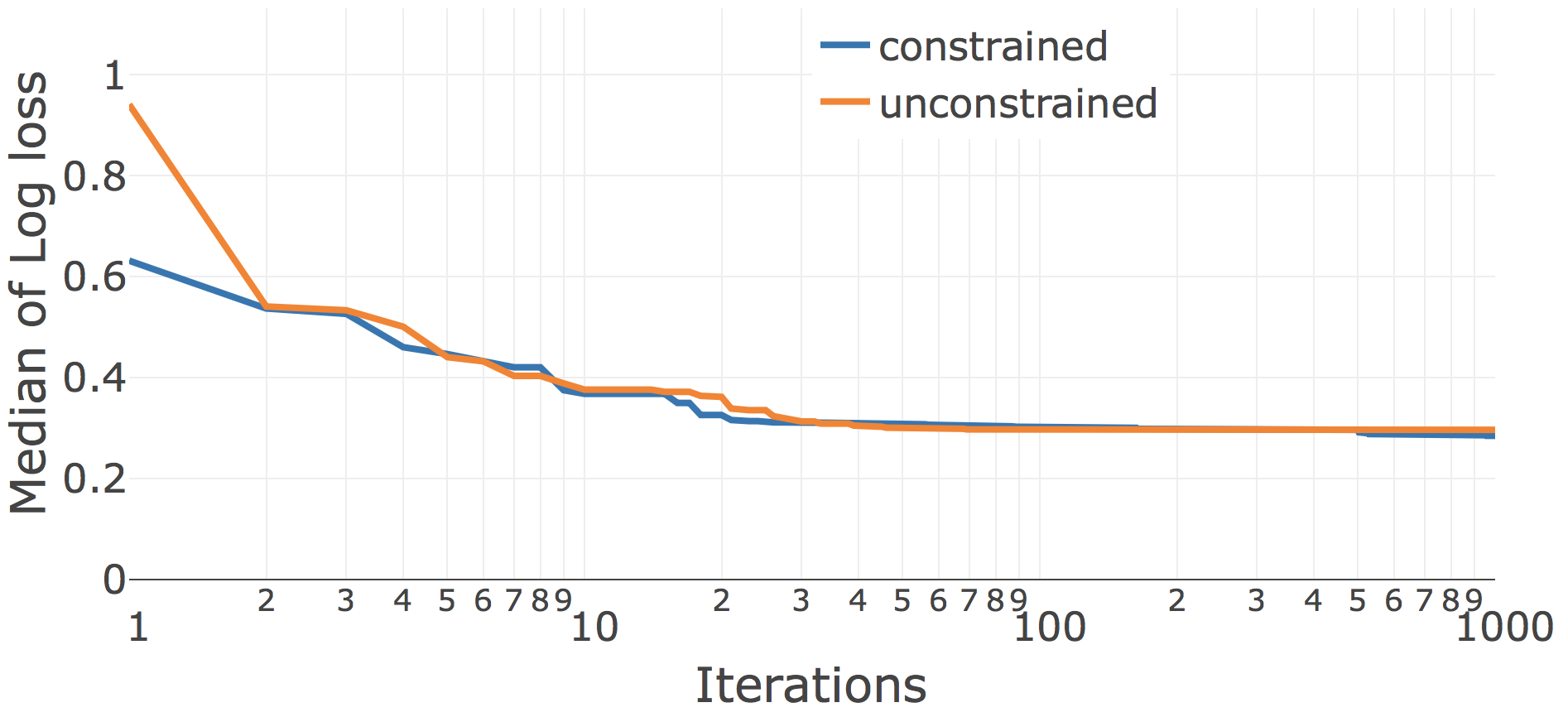
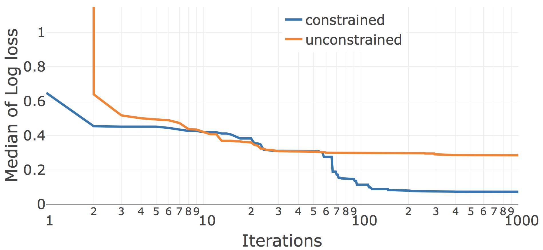
Lale’s search space compiler takes rich hyperparameter schemas including side constraints and translates them into semantically equivalent search spaces for different AutoML tools. This raises the question of how important those side constraints are in practice. To explore this, we did an ablation study where we generated not just the constrained search spaces that are default with Lale but also unconstrained search spaces that drop side constraints. With hyperopt on the unconstrained search space, some iterations are unsuccessful due to exceptions, for which we reported np.float.max loss. Figure 14 plots the convergence for the Car dataset on the planned pipeline LR | KNN. Both of these operators have a few side constraints. Whereas the unconstrained search space causes some invalid points early in the search, the two curves more-or-less coincide after about two dozen iterations. The story looks very different in Figure 14 when adding a third operator J48 | LR | KNN. In the unconstrained case, J48 has many more invalid runs, causing hyperopt to see so many np.float.max loss values from J48 that it gives up on it. In the constrained case, on the other hand, J48 has no invalid runs, and hyperopt eventually realizes that it can configure J48 to obtain substantially better performance.
6.4. Dataset Details
In order to be specific about the exact datasets for reproducibility, Table 3 report the URLs for accessing those.
| Dataset | URL |
|---|---|
| australian | https://www.openml.org/d/40981 |
| blood | https://www.openml.org/d/1464 |
| breast-cancer | https://www.openml.org/d/13 |
| car | https://www.openml.org/d/40975 |
| credit-g | https://www.openml.org/d/31 |
| diabetes | https://www.openml.org/d/37 |
| hill-valley | https://www.openml.org/d/1479 |
| jungle-chess | https://www.openml.org/d/41027 |
| kc1 | https://www.openml.org/d/1067 |
| kr-vs-kp | https://www.openml.org/d/3 |
| mfeat-factors | https://www.openml.org/d/12 |
| phoneme | https://www.openml.org/d/1489 |
| shuttle | https://www.openml.org/d/40685 |
| spectf | https://www.openml.org/d/337 |
| sylvine | https://www.openml.org/d/41146 |
| CIFAR-10 | https://en.wikipedia.org/wiki/CIFAR-10 |
| Drug Review | https://archive.ics.uci.edu/ml/datasets/Drug+Revi+Dataset+%28Drugs.com%29 |
| Epilepsy | https://www.ncbi.nlm.nih.gov/pmc/articles/PMC6246677 |
7. Related Work
There are various search tools, designed around scikit-learn (Buitinck et al., 2013), and each usually focused on a particular novel optimization algorithm. Auto-sklearn (Feurer et al., 2015) uses the search space specification and optimization algorithm of SMAC (Hutter et al., 2011). Hyperopt-sklearn (Komer et al., 2014) uses its own search space specification scheme and a novel optimizer based on Tree-structured Parzen Estimators (TPE) (Bergstra et al., 2011). Scikit-learn also comes with its own GridSearchCV and RandomizedSearchCV classes. Auto-Weka (Thornton et al., 2013) is a predecessor of auto-sklearn that also uses SMAC but operates on operators from Weka (Hall et al., 2009) instead of scikit-learn. TPOT (Olson et al., 2016) is designed around scikit-learn and uses genetic programming to search for pipeline topologies and operator choices. This usually leads to the generation of many misconfigured pipelines, wasting execution time. RECIPE (de Sá et al., 2017) prunes away the misconfigurations to save execution time by validating generated pipelines with a grammar for linear pipelines. AlphaD3M (Drori et al., 2019) makes use of a grammar in a generative manner (instead of just for validation) with a deep reinforcement learning based algorithm. Katz et al. (Katz et al., 2020) similarly use a grammar for Lale pipelines with AI planning tools. In contrast to these tools, the contribution of this paper is not a novel optimization algorithm but rather a more consistent programming model with search space generation targeting existing tools.
8. Conclusion
This paper describes Lale, a library for semi-automated data science. Lale contributes a syntax that is consistent with scikit-learn, but extends it to support a broad spectrum of automation including algorithm selection, hyperparameter tuning, and topology search. Lale works by automatically generating search spaces for established AutoML tools, extending their capabilities to grammar-based search and to search inside higher-order operators. The experiments show that search spaces crafted using Lale achieve results that are competitive with state-of-the-art tools while offering more versatility.
References
- (1)
- Baudart et al. (2019) Guillaume Baudart, Martin Hirzel, Kiran Kate, Louis Mandel, and Avraham Shinnar. 2019. Machine Learning in Python with No Strings Attached. In Workshop on Machine Learning and Programming Languages (MAPL). 1–9. https://doi.org/10.1145/3315508.3329972
- Baudart et al. (2020) Guillaume Baudart, Peter Kirchner, Martin Hirzel, and Kiran Kate. 2020. Mining Documentation to Extract Hyperparameter Schemas. In ICML Workshop on Automated Machine Learning (AutoML@ICML). https://arxiv.org/abs/2006.16984
- Bergstra et al. (2011) James Bergstra, Rémi Bardenet, Yoshua Bengio, and Balázs Kégl. 2011. Algorithms for Hyper-Parameter Optimization. In Conference on Neural Information Processing Systems (NIPS). http://papers.nips.cc/paper/4443-algorithms-for-hyper-parameter-optimizat
- Bergstra et al. (2015) James Bergstra, Brent Komer, Chris Eliasmith, Dan Yamins, and David D. Cox. 2015. Hyperopt: a Python Library for Model Selection and Hyperparameter Optimization. Computational Science & Discovery 8, 1 (2015). http://dx.doi.org/10.1088/1749-4699/8/1/014008
- Buitinck et al. (2013) Lars Buitinck, Gilles Louppe, Mathieu Blondel, Fabian Pedregosa, Andreas Mueller, Olivier Grisel, Vlad Niculae, Peter Prettenhofer, Alexandre Gramfort, Jaques Grobler, Robert Layton, Jake VanderPlas, Arnaud Joly, Brian Holt, and Gaël Varoquaux. 2013. API Design for Machine Learning Software: Experiences from the scikit-learn Project. https://arxiv.org/abs/1309.0238
- Chen and Guestrin (2016) Tianqi Chen and Carlos Guestrin. 2016. XGBoost: A Scalable Tree Boosting System. In Conference on Knowledge Discovery and Data Mining (KDD). 785–794. http://doi.acm.org/10.1145/2939672.2939785
- Chomsky (1956) Noam Chomsky. 1956. Three models for the description of language. IRE Transactions on Information Theory 2, 3 (1956), 113–124.
- de Sá et al. (2017) Alex G. C. de Sá, Walter José G. S. Pinto, Luiz Otavio V. B. Oliveira, and Gisele L. Pappa. 2017. RECIPE: A Grammar-Based Framework for Automatically Evolving Classification Pipelines. In European Conference on Genetic Programming (EuroGP). 246–261. https://link.springer.com/chapter/10.1007/978-3-319-55696-3_16
- Drori et al. (2019) Iddo Drori, Yamuna Krishnamurthy, Raoni Lourenco, Remi Rampin, Kyunghyun Cho, Claudio Silva, and Juliana Freire. 2019. Automatic Machine Learning by Pipeline Synthesis using Model-Based Reinforcement Learning and a Grammar. In Workshop on Automatic Machine Learning (AutoML). https://www.automl.org/wp-content/uploads/2019/06/automlws2019_Paper34.pdf
- Feurer et al. (2015) Matthias Feurer, Aaron Klein, Katharina Eggensperger, Jost Springenberg, Manuel Blum, and Frank Hutter. 2015. Efficient and Robust Automated Machine Learning. In Conference on Neural Information Processing Systems (NIPS). 2962–2970. http://papers.nips.cc/paper/5872-efficient-and-robust-automated-machine-learning
- Hall et al. (2009) Mark Hall, Eibe Frank, Geoffrey Holmes, Bernhard Pfahringer, Peter Reutemann, and Ian H. Witten. 2009. The WEKA Data Mining Software: An Update. SIGKDD Explorations Newsletter 11, 1 (Nov. 2009), 10–18. http://doi.acm.org/10.1145/1656274.1656278
- Hutter et al. (2011) Frank Hutter, Holger H. Hoos, and Kevin Leyton-Brown. 2011. Sequential Model-Based Optimization for General Algorithm Configuration. In International Conference on Learning and Intelligent Optimization (LION). 507–523. https://doi.org/10.1007/978-3-642-25566-3_40
- Katz et al. (2020) Michael Katz, Parikshit Ram, Shirin Sohrabi, and Octavian Udrea. 2020. Exploring Context-Free Languages via Planning: The Case for Automating Machine Learning. In International Conference on Automated Planning and Scheduling (ICAPS), Vol. 30. 403–411. https://www.aaai.org/ojs/index.php/ICAPS/article/view/6686
- Ke et al. (2017) Guolin Ke, Qi Meng, Thomas Finley, Taifeng Wang, Wei Chen, Weidong Ma, Qiwei Ye, and Tie-Yan Liu. 2017. LightGBM: A highly efficient gradient boosting decision tree. In Conference on Neural Information Processing Systems (NIPS). 3146–3154. http://papers.nips.cc/paper/6907-lightgbm-a-highly-efficient-gradient-boosting-decision-tree.pdf
- Komer et al. (2014) Brent Komer, James Bergstra, and Chris Eliasmith. 2014. Hyperopt-Sklearn: Automatic Hyperparameter Configuration for Scikit-Learn. In Python in Science Conference (SciPy). 32–37. http://conference.scipy.org/proceedings/scipy2014/komer.html
- Liu et al. (2020) Sijia Liu, Parikshit Ram, Deepak Vijaykeerthy, Djallel Bouneffouf, Gregory Bramble, Horst Samulowitz, Dakuo Wang, Andrew Conn, and Alexander G Gray. 2020. An ADMM Based Framework for AutoML Pipeline Configuration. In Conference on Artificial Intelligence (AAAI). 4892–4899. https://aaai.org/ojs/index.php/AAAI/article/view/5926
- Olson et al. (2016) Randal S. Olson, Ryan J. Urbanowicz, Peter C. Andrews, Nicole A. Lavender, La Creis Kidd, and Jason H. Moore. 2016. Automating Biomedical Data Science Through Tree-Based Pipeline Optimization. In European Conference on the Applications of Evolutionary Computation (EvoApplications). 123–137. https://doi.org/10.1007/978-3-319-31204-0_9
- Pezoa et al. (2016) Felipe Pezoa, Juan L. Reutter, Fernando Suarez, Martín Ugarte, and Domagoj Vrgoč. 2016. Foundations of JSON Schema. In International Conference on World Wide Web (WWW). 263–273. https://doi.org/10.1145/2872427.2883029
- Schindler et al. (2006) Kaspar Schindler, Howan Leung, Christian E. Elger, and Klaus Lehnertz. 2006. Assessing seizure dynamics by analysing the correlation structure of multichannel intracranial EEG. Brain 130, 1 (11 2006), 65–77. arXiv:http://oup.prod.sis.lan/brain/article-pdf/130/1/65/992272/awl304.pdf https://doi.org/10.1093/brain/awl304
- Thornton et al. (2013) Chris Thornton, Frank Hutter, Holger H. Hoos, and Kevin Leyton-Brown. 2013. Auto-WEKA: Combined Selection and Hyperparameter Optimization of Classification Algorithms. In Conference on Knowledge Discovery and Data Mining (KDD). 847–855. https://doi.org/10.1145/2487575.2487629