LaplacianFusion: Detailed 3D Clothed-Human Body Reconstruction
Abstract.
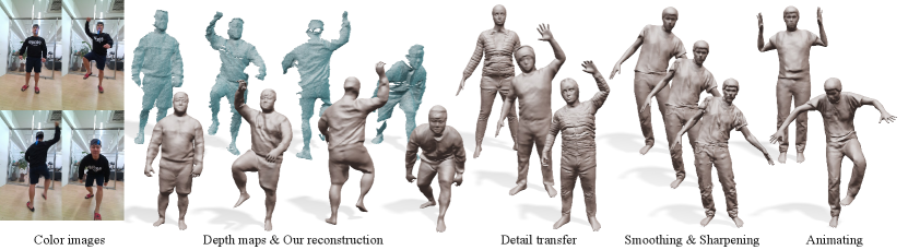
We propose LaplacianFusion, a novel approach that reconstructs detailed and controllable 3D clothed-human body shapes from an input depth or 3D point cloud sequence. The key idea of our approach is to use Laplacian coordinates, well-known differential coordinates that have been used for mesh editing, for representing the local structures contained in the input scans, instead of implicit 3D functions or vertex displacements used previously. Our approach reconstructs a controllable base mesh using SMPL, and learns a surface function that predicts Laplacian coordinates representing surface details on the base mesh. For a given pose, we first build and subdivide a base mesh, which is a deformed SMPL template, and then estimate Laplacian coordinates for the mesh vertices using the surface function. The final reconstruction for the pose is obtained by integrating the estimated Laplacian coordinates as a whole. Experimental results show that our approach based on Laplacian coordinates successfully reconstructs more visually pleasing shape details than previous methods. The approach also enables various surface detail manipulations, such as detail transfer and enhancement.
1. Introduction
3D reconstruction of clothed human models is crucial for reproducing digital twins of real world to give the user a sense of reality and immersion. Clothed human models are useful for various applications, such as entertainment, virtual reality, and the movie industry. In particular, with the surging demands for social connections in virtual spaces, it is valuable to produce realistic 3D human models in a typical capturing setup.
Parametric human models have been proposed to reconstruct 3D full body shapes for different poses. Among them, SMPL (Loper et al., 2015) is a representative model and represents a human model with shape and pose parameters that are applied to a single template mesh with fixed topology. In SMPL, shape deformations are obtained by linear blend skinning of the template mesh and cannot be detailed enough for depicting surface details of clothed human models. This limitation also applies to other parametric models of human shapes (Joo et al., 2018; Pavlakos et al., 2019).
Recent learning-based methods for clothed human reconstruction utilize implicit 3D functions (Saito et al., 2021; Wang et al., 2021), but they learn a function defined in a 3D space and need an additional polygon extraction step to provide a 3D mesh as the output. An explicit point cloud representation has been used to reconstruct loose clothes (Ma et al., 2021b, a), but this approach also needs the surface reconstruction step to produce a 3D mesh that can be directly used for applications. On the other hand, Burov et al. (2021) use an explicit mesh representation and train a Dynamic Surface Function Network (DSFN) to estimate vertex displacements for a template mesh. However, DSFN may not fully exploit the surface details in the input scans due to the spatial regularization constraint needed for training.
In this paper, we present LaplacianFusion, a novel framework that reconstructs a detailed and controllable 3D clothed human model from an input depth or point cloud sequence. Our key idea is to use differential coordinates, instead of implicit 3D function or vertex displacements, for representing local structures of surface details. For the differential coordinates, we use Laplacian coordinates (Karni and Gotsman, 2000; Alexa, 2003; Sorkine et al., 2003) that have been widely applied to mesh processing and editing (Lipman et al., 2004; Sorkine et al., 2004). Intuitively, Laplacian coordinates are the difference between a point and the average of its neighbors, so they can naturally encode local shape variations.
In our LaplacianFusion framework, the reconstructed human model is expressed as combination of a controllable base mesh and a surface function using a multi-layer perceptron (MLP). In the training phase, we first reconstruct a base mesh sequence based on SMPL that fits the input scans. We then train an MLP function by fusing the Laplacian values estimated at input points on the surface of the SMPL template mesh. As a result, the MLP function learns to predict Laplacian coordinates representing the details on the body surface. To reconstruct a detailed human model for a given pose, we start from a SMPL template mesh in the canonical space and obtain a base mesh by deforming the SMPL template using the pose parameters. We then subdivide the base mesh to have enough vertices and estimate Laplacian coordinates for the vertices using the learned MLP function. Finally, the detailed output mesh is obtained by globally integrating the estimated Laplacian coordinates as a whole. In this paper, we call the MLP function neural surface Laplacian function.
We aim for a natural capture scenario where the subject freely performs actions during the capture. Our approach can handle both full and partial views of point clouds that are captured by a dome-shaped multi-camera setup (Collet et al., 2015) and a single RGB-D camera (Kin, 2022), respectively. The reconstructed 3D models are controllable as the base mesh and the neural surface Laplacian function are conditioned on SMPL pose parameters. Our approach restores the surface details of a clothed human body better than the recent explicit surface-based approach, DSFN (Burov et al., 2021). In addition, due to the differential representation and a fixed-topology base mesh, our approach can be easily adapted for other applications, including detail transfer, detail enhancement, and texture transfer. Our codes are publicly available.111https://github.com/T2Kim/LaplacianFusion
Our main contributions can be summarized as follows:
-
•
We propose LaplacianFusion, a novel framework for reconstructing surface details of a clothed human body model. Our framework can handle both partial and full-body point cloud sequences.
-
•
We introduce an approach to learn Laplacian coordinates representing surface details from scanned points using a MLP.
-
•
Our reconstructed model is controllable by pose parameters and supports various shape manipulations, including detail transfer.
2. Related Work
2.1. Parametric models for 3D human shapes and clothes
Human body models
PCA-based parametric models have been proposed for handling human body and pose variations: SMPL (Loper et al., 2015; Romero et al., 2017; Pavlakos et al., 2019), GHUM (Xu et al., 2020), and Frank model (Joo et al., 2018). These models can handle body shape variations and pose-dependent shape deformations that cannot be modeled with Linear Blend Skinning (LBS) (Lewis et al., 2000). The models are suitable for expressing human shapes with coarse meshes, but they alone are not enough for containing rich details.
Clothed human models
Several approaches represented clothed humans by extending parametric human models. SMPL (Loper et al., 2015) has been extended to express clothed deformations by directly adding a displacement vector to each vertex (Alldieck et al., 2019, 2018a, 2018b; Bhatnagar et al., 2020). CAPE (Ma et al., 2020) proposed an extended model by adding a cloth style term to SMPL. Other approaches (De Aguiar et al., 2010; Guan et al., 2012; Pons-Moll et al., 2017; Bhatnagar et al., 2019; Tiwari et al., 2020; Xiang et al., 2020) used additional parametric models for representing clothes on top of a parametric human model. Additional approaches for expressing surface details include GAN-based normal map generation (Lahner et al., 2018), RNN-based regression (Santesteban et al., 2019), and style-shape specific MLP functions (Patel et al., 2020). However, these approaches are limited to several pre-defined clothes and cannot recover detailed human shapes with arbitrary clothes from input scans.
2.2. Implicit clothed human reconstruction
Volumetric implicit representations
Truncated signed distance function (TSDF) is a classical implicit representation for reconstruction. TSDF-based approaches that warp and fuse the input depth sequence onto the canonical volume have been proposed for recovering dynamic objects (Newcombe et al., 2015; Innmann et al., 2016). This volume fusion mechanism is extended to be conditioned with the human body prior for representing a clothed human (Yu et al., 2017; Tao et al., 2018). Optimized approaches for real-time performance capture have also been proposed (Dou et al., 2016; Dou et al., 2017; Habermann et al., 2020; Yu et al., 2021).
Neural implicit representations
MLP-based neural implicit representation has been actively investigated for object reconstruction (Park et al., 2019; Mescheder et al., 2019; Chen and Zhang, 2019). PIFu (Saito et al., 2019; Saito et al., 2020) firstly adopted this representation for reconstructing static clothed human from a single image. DoubleField (Shao et al., 2022) uses multi-view RGB cameras and improves visual quality by sharing the learning space for geometry and texture. With depth image or point cloud input, multi-scale features (Chibane et al., 2020; Bhatnagar et al., 2020) and human part classifiers (Bhatnagar et al., 2020) have been used for reconstructing 3D human shapes. Li et al. (2021b) proposed implicit surface fusion from a depth stream and enabled detailed reconstruction even for invisible regions.
Neural parametric models have also been proposed for modeling shape and pose deformations. NASA (Deng et al., 2020) learns pose-dependent deformations using part-separate implicit functions. LEAP (Mihajlovic et al., 2021) and imGHUM (Alldieck et al., 2021) learn parametric models that can recover shape and pose parameters for SMPL (Loper et al., 2015) and GHUM (Xu et al., 2020), respectively. NPMs (Palafox et al., 2021) encodes shape and pose variations into two disentangled latent spaces using auto-decoders (Park et al., 2019). SPAMs (Palafox et al., 2022) introduces a part-based disentangled representation of the latent space.
For subject-specific clothed human reconstruction from scans, recent implicit methods define shape details in a canonical shape and use linear blend skinning to achieve both detail-preservation and controllability. Neural-GIF (Tiwari et al., 2021) learns a backward mapping network for mapping points to the canonical space and a displacement network working in the canonical space. In contrast, SNARF (Chen et al., 2021) proposed a forward skinning network model to better handle unseen poses. SCANimate (Saito et al., 2021) learns forward and backward skinning networks with a cycle loss to reconstruct disentangled surface shape and pose-dependent deformations. MetaAvatar (Wang et al., 2021) proposed an efficient pipeline for subject-specific fine-tuning using meta-learning.
These implicit representations are topology-free and can handle vastly changing shapes, such as loose clothes. However, they individually perform shape reconstruction at every frame and cannot provide temporally consistent mesh topology needed for animation. In addition, this approach needs dense point sampling in a 3D volume to train implicit functions and is computationally heavy.
| Method | Shape representation |
2.5D input |
3D input |
Animation ready |
Texture map ready |
|
| Implicit | DynamicFusion (2015) | SDF | ✓ | |||
| BodyFusion (2017) | SDF | ✓ | ||||
| NASA (2020) | Occupancy | ✓ | ✓ | |||
| IF-Net (2020) | Occupancy | ✓ | ✓ | |||
| IP-Net (2020) | Occupancy | ✓ | ✓ | ✓ | ||
| NPMs (2021) | SDF | ✓ | ✓ | ✓ | ||
| Neural-GIF (2021) | SDF | ✓ | ✓ | |||
| SCAnimate (2021) | SDF | ✓ | ✓ | |||
| MetaAvatar (2021) | SDF | ✓ | ✓ | ✓ | ||
| SNARP (2021) | SDF | ✓ | ✓ | |||
| POSEFusion (2021b) | Occupancy | ✓ | ✓ | |||
| LEAP (2021) | Occupancy | ✓ | ✓ | |||
| Explicit | CAPE (2020) | Coord. (vertex) | ✓ | ✓ | ✓ | |
| SCALE (2021a) | Coord. (patch) | ✓ | ✓ | |||
| PoP (2021b) | Coord. (point) | ✓ | ✓ | |||
| DSFN (2021) | Coord. (vertex) | ✓ | ✓ | ✓ | ||
| Ours | Coord. + Laplacian | ✓ | ✓ | ✓ | ✓ |
2.3. Explicit clothed human reconstruction.
Explicit representations for reconstructing clothed humans have been developed mainly for handling geometric details on the template mesh of a parametric model such as SMPL (Loper et al., 2015).
Point-based
SCALE (Ma et al., 2021a) recovers controllable clothed human shapes by representing local details with a set of points sampled on surface patches. To avoid artifacts of the patch-based approach at patch boundaries, PoP (Ma et al., 2021b) represents local details using point samples on a global 2D map. Point cloud representation has a flexible topology and can cover more geometric details. However, this representation does not provide an explicit output mesh.
Mesh-based
For subject-specific human reconstruction with a depth sequence, DSFN (Burov et al., 2021) represents surface details using vertex offsets on a finer resolution mesh obtained by subdividing the SMPL template mesh. This approach is the closest to ours. The main difference is that our method represents surface details using Laplacian coordinates, instead of vertex offsets. Experimental results show that Laplacian coordinates are more effective for recovering surface details than vertex offsets (Section 8).
Table 1 compares our method with related ones in terms of possible inputs and desirable properties.
3. Preliminary
3.1. Laplacian coordinates from a mesh
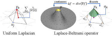
In the graphics literature, recovering an unknown function from differential quantities (Laplacian) has become widely known through Poisson image editing (Pérez et al., 2003). This technique was successfully expanded to the 3D mesh domain, especially for mesh editing (Lipman et al., 2004; Sorkine et al., 2004). In mesh editing, the differential quantities are used to encode vertex coordinates and called Laplacian coordinates. Mesh editing based on Laplacian coordinates includes three steps: Encoding Laplacian coordinates from the original mesh, interactive editing of control points, and converting Laplacian coordinates into absolute vertex positions of the target mesh while satisfying the positional constraints imposed by edited control points. In the following, we briefly introduce the encoding and converting steps.
Let the original mesh be described by the vertex set and the triangle set , where . denotes the position of the -th vertex and is the number of vertices. Uniform Laplacian coordinates are defined by:
| (1) |
where indicates uniform weights, and denotes the set of adjacent vertices of the -th vertex (Figure 2 left). Regarding all vertices, this equation can be represented in a matrix form: , where is the uniform Laplacian matrix. Notably, the matrix has rank , so can be converted into by taking the specified position of a selected vertex as the boundary condition and solving a linear system. For example, when fixing the -th vertex, we can form a sparse linear system , where and . denotes one-hot encoding, where the -th element is one.
3.2. Laplacian coordinates from a point cloud
In this paper, we compute Laplacian coordinates from raw 3D scan data and use them for shape detail reconstruction. Then, we need an alternative approach to Eq. (1) for computing Laplacian coordinates as a point cloud does not have edge connectivity. We may consider directly building edges from the point set, but it may generate a noisy and non-manifold mesh. To resolve this difficulty, Liang et al. (2012) defined the Laplace-Beltrami operator on a point cloud by fitting a quadratic function for the local neighborhood of a point and computing the differentials of the function (Figure 2 middle). However, the Laplace-Beltrami operator computes Laplacian coordinates using a continuous function that reflects the non-uniform local shape in the neighborhood, which differs from the discrete uniform Laplacian coordinates in Eq. (1). Therefore, Laplacian coordinates calculated by the Laplace-Beltrami operator need to be converted into mesh’s vertex positions differently.
Let’s assume that we have a mesh . We can calculate the discrete Laplace-Beltrami operator on the mesh (Figure 2 right) as follows (Meyer et al., 2003):
| (2) |
where is non-uniform Laplacian coordinates, is the discrete Laplace-Beltrami operator, denotes cotangent function, is the Voronoi area of , and and are the two angles opposite to the edge on . Similarly to Eq. (1), Eq. (2) can be represented in a matrix form , where is the non-uniform Laplacian matrix, and we can convert into by solving a linear system with a boundary condition.
Compared with global coordinates, which represent exact spatial locations, Laplacian coordinates naturally encode local shape information, such as the sizes and orientations of local details (Sorkine, 2006). In mesh editing, this property has been used to retain desirable local shapes during the editing process by encoding Laplacian coordinates from the original mesh and constraining the edited mesh to follow the encoded Laplacian coordinates. In this paper, we use the property for shape reconstruction rather than editing. We extract and encode the local details from the input scan data using Laplacian coordinates and restore the desirable details on the subdivided base mesh by integrating the encoded Laplacian coordinates.
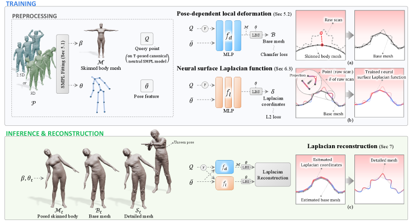
4. Overview
Figure 3 shows the overall process of our LaplacianFusion framework. The input is a sequence of point clouds , each of which contains either 2.5D depth map or 3D full scan of a clothed human body with motion. Our pipeline starts from the SMPL template mesh in the canonical T-pose (Section 5.1). SMPL provides the shape prior for the reconstructed models and enables the controllability using pose parameters. Given an input sequence, we estimate a single SMPL shape parameter and per-frame SMPL pose parameters , and obtain the posed skin body for each frame . Since the mesh may not accurately fit the input point cloud, we add pose-dependent local deformations to improve the fitting and obtain the base mesh (Section 5.2), where the local deformations are estimated using an MLP function that computes vertex displacements for . On top of the base mesh , our novel neural surface Laplacian function predicts Laplacian coordinates that encode the surface details of a clothed human model (Section 6). Finally, we reconstruct the detailed output mesh by integrating Laplacian coordinates estimated at the vertices of the subdivided base mesh (Section 7). Note that and are functions of both 3D positions and pose parameters as the local deformations and cloth details such as wrinkles are pose-dependent. We outline the training and inference phases for the two surface functions below.
Training phase
We sequentially train the two surface functions because 3D points on a base mesh obtained by are used as the input of . We train to learn a deformation field that minimizes the Chamfer distance (Barrow et al., 1977) between the input point cloud and the base mesh . To train , for each point in the input point cloud, we calculate approximate Laplacian coordinates as described in Section 3.2, and find the corresponding point on the base mesh to assign the calculated Laplacian coordinates. is then trained to learn the assigned Laplacian coordinates on by mininmizing the L2 loss.
Inference phase
We can infer the surface details for a particular pose using the learned MLP functions and . We first obtain the posed skinned body by applying the given pose parameter to the SMPL template mesh. We then apply the local deformation function to and obtain the pose-dependent base mesh . Since the vertex number of the SMPL template is insufficient to represent surface details of a clothed human, we subdivide the base mesh . We estimate Laplacian coordinates for each vertex of the subdivided using neural surface Laplacian function . Finally, we reconstruct a detailed clothed human model by integrating the estimated Laplacian coordinates. Note that the pose parameter used in the inference phase can be arbitrary, and it does not have to be one of the pose parameters estimated from the input frames (Section 8.4).
5. Pose-dependent base mesh
5.1. Skinned body acquisition
Our approach starts with building a skinned body. We adopt the SMPL model (Loper et al., 2015) that can readily manipulate 3D human shape using identity-dependent parameters and pose-dependent parameters . SMPL supports rigging and skinning, and the template mesh can be deformed with an arbitrary pose. As in the SMPL model, we use the linear blend skinning (LBS) scheme (Lewis et al., 2000) to compute template mesh deformation:
| (3) |
where denotes the index of a joint, is the number of joints, denotes a rigid transformation matrix for the -th joint, is a skinning weight vector of predefined by SMPL model, and is homogeneous vertex coordinates of the base mesh. We can conduct articulated deformation by applying Eq. (3) to all mesh vertices.
The canonical neutral SMPL model is in the T-pose, and we align the model with each input point cloud by estimating shape and pose parameters, and , so that the constructed posed skinned body can fit well. We apply deep virtual markers (Kim et al., 2021) to and to obtain the initial geometric correspondence. We additionally use OpenPose (Cao et al., 2019) to improve the point matching accuracy if color images are available. To obtain the parameters and for , we optimize them using the initial correspondence between and , and then further minimize the correspondence alignment error and the Chamfer distance together. We add the smoothness regularization term in temporal domain for the optimization so that SMPL’s pose parameters can be changed gradually.
In the face region of the SMPL model, vertices are placed with uneven distribution to provide a detailed face. However, such distribution does not match with the almost uniform point distributions in the input raw scans. Therefore, we re-mesh the face region of the SMPL model, and the skinning weights of new vertices are assigned from the nearest original vertices.
5.2. Pose-dependent base mesh
Suppose we have obtained a skinned body mesh that approximates the input frame from the previous step. To fit the SMPL model tighter to the input point cloud, we combine pose-dependent local deformation with (Figure 3a), and obtain a pose-dependent base mesh ;
| (4) |
where is a vertex of . In Eq. (4), the displacements are applied to the vertices of the T-posed SMPL mesh with the optimized shape parameter before the articulated deformation is performed using LBS function. accounts for pose-dependent local deformation and is implemented as an MLP. takes as the input a query point and a per-point pose feature that are described in Section 6.1. We observe such local deformations are useful to handle large shape variations in the input scans.
To optimize , we formulate an energy function as follows:
| (5) |
where is a target point in the point cloud at frame , evaluates Chamfer distance from to , and indicates the base mesh for which SMPL pose parameter and pose-dependent local deformation are applied: , where and denotes the -th vertex deformed by Eq. (4) with . is a weight parameter. In all equations, for simplicity, we omit averaging terms that divide the sum of Chamfer distances by the number of points.
In Eq. (5), per-point weight is used to fully exploit geometric details captured in the input depth images. Details of nearer objects to the camera are usually better captured than farther ones, and it is advantageous to put more weights on the input points closer to the camera. We then use , where is the depth value of at frame and the parameter is set to 2. If the input is a sequence of point clouds, where the distance to the camera is not clear, we use .
To avoid noisy artifact, we use Laplacian regularizer in Eq. (5) that is defined by
| (6) |
where is the set of adjacent vertices of the -th vertex. regularizes the shape of a base mesh to be smooth. During training time, we construct the total energy by gathering the per-frame energies of randomly sampled frames and optimize the total energy using Adam optimizer (Kingma and Ba, 2015).
Note that, in contrast to DSFN (Burov et al., 2021), we do not conduct any mesh subdivision at this stage for efficiency. Indeed, in our experiments, SMPL topology is sufficient to represent a coarse, smooth mesh that is needed for learning neural surface Laplacian function in the following section.
6. Neural surface Laplacian function
To fully exploit the fine-level details in the input point cloud, we construct a neural surface Laplacian function that is an MLP defined on the surface of a pose-dependent base mesh . The input of is the same as for , but the output is approximate Laplacian coordinates, whereas produces a displacement vector.
6.1. Function input
Query point
In the inputs of functions and , we use the concept of query point to neutralize shape variations of the base meshes for different subjects and at different frames. We define a query point as a 3D point on the T-posed canonical neutral SMPL model . Consider two base meshes and for the same subject at different frames and their -th vertices and , respectively. 3D positions of and may differ, but their query points and are defined to be same as they share the same vertex index (Figure 4a). Similarly, is defined to be the same for the vertices of base meshes representing different subjects if the vertices have been deformed from the same vertex of . In addition, can be defined for any point on a base mesh other than vertices by using the barycentric coordinates in the mesh triangles. Once determined, a query point is converted to a high-dimensional vector via a positional encoding (Mildenhall et al., 2020), and we choose the dimension of ten in our experiments.
 |
 |
| (a) Query point | (b) Pose feature |
Pose feature
For a query point, our two MLPs and should estimate pose-dependent deformation and Laplacian coordinates, respectively. To provide the pose-dependency, we could simply include the pose parameter in the input of the MLPs. However, a query point is not affected by every joint but strongly associated with nearby joints. For example, the joint angle at the shoulder is irrelevant to local details on a leg. To exploit the correlations between query points and joint angles in a pose parameter , we convert to a per-point pose feature that retains only relevant joint angles for a query point . Inspired by Pose Map (Saito et al., 2021), we apply the joint association weight map and skinning weights of to the original pose parameter . Our pose feature used as the input of MLPs is defined by
| (7) |
where converts an input vector to a diagonal matrix, and is an element-wise ceiling operation. We manually define the weight map to reflect our setting. For example, the details of the head are not correlated with any joint in our reconstructed model, and the details of a leg are affected by all nearby joints together. Then, for the head joint, we set zero for the association weight of any joint in . For a joint around a leg, we set higher association weights for all nearby joints (Figure 4b).
6.2. Training pairs
To train the neural surface Laplacian function , we calculate the ground-truth (GT) approximate Laplacian coordinates of scan points and localize them on to the corresponding query points.
GT Laplacian coordinates approximation
As discussed in Section 3.2, we use an approximation method (Liang et al., 2012) for calculating Laplacian coordinates from scan points that do not have connectivity. We first locally fit a degree two polynomial surface for each point in the moving least squares manner. In our experiments, we use 20-30 neighbor points for the local surface fitting. Figure 5 shows illustration. Our approximate Laplacian coordinates are defined on a continuous domain, unlike in conventional mesh editing methods (Lipman et al., 2004; Sorkine et al., 2004) that formulate Laplacian coordinates in a discrete domain using mesh vertices. To apply our Laplacian coordinates to a discrete mesh, we take advantage of a pose-dependent base mesh (Section 7).
 |
 |
|
| (a) Scan | (b) Local coordinate system | (c) Quadric surface |
Localization
Although the base mesh nearly fits the input point cloud, points may not reside exactly on the mesh. To obtain the corresponding query point, we project each point in the input point cloud onto the base mesh : , where denotes the projection operation from a point to a pose-dependent base mesh (Figure 3b). The position of is determined by the barycentric coordinates in a triangle of , so we can easily compute the query point, skinning weights, and pose feature using the barycentric weights.
6.3. Optimization
neural surface Laplacian function
For a given surface point and pose , the MLP estimates Laplacian coordinates:
| (8) |
The estimation is conducted in the canonical space and transformed into the posed space. Working in the canonical space is essential because Laplacian coordinates are not invariant to rotation. In Eq. (8), we discard the translation part in Eq. (3) as Laplacian coordinates are differential quantity. The estimated is non-uniform Laplacian coordinates, as described in Section 3.2.
We train the MLP by formulating a per-point energy function:
| (9) |
where is the Laplacian coordinates of predicted by using Eq. (8), is the GT approximate Laplacian coordinates of , and is the weight used in Eq. (5). During training, we construct the total energy by summing per-point energies of randomly sampled input points, and optimize the total energy using Adam optimizer (Kingma and Ba, 2015).
7. Laplacian Reconstruction
Once the training is over, for a given pose , we can obtain the pose-dependent base mesh and the Laplacian coordinates for the vertices of . In the reconstruction step, we aggregate the estimated Laplacian coordinates to restore a whole body model.
Subdivision
For detailed surface reconstruction, we subdivide the base mesh as the SMPL model does not have enough number of vertices for representing fine details. The new vertices of the subdivided mesh reside on the midpoints of edges of . We conduct subdivision twice, and the number of triangles increases 16 times. As a result, we have the subdivided pose-dependent base mesh , where and is the number of vertices of .
Reconstruction
Using the base mesh , as illustrated in Figure 3c, we reconstruct a detailed mesh , where , by minimizing the following error functional (Lipman et al., 2004; Sorkine et al., 2004):
| (10) |
where is the Laplace-Beltrami operator of defined in Eq. (2), is the non-uniform Laplacian coordinates of predicted by the neural surface Laplacian function using Eq. (8), and is a set of indices of the constraint vertices on , which play the role of boundary conditions. In Eq. (10), the first term preserves desirable Laplacian coordinates on the whole surface, and the second term constrains the global position of the final shape using the anchor points.
Laplace-Beltrami operator
To compute the Laplace-Beltrami operator using Eq. (2), we need the angles and for each edge connecting vertices and in . For efficient computation, we use uniform angle for all edges of . Then, Eq. (2) is reduced to
| (11) |
where is the Voronoi area of a vertex of . As shown in the experimental results (Section 8), this approximation successfully reconstructs from the predicted non-uniform Laplacian coordinates.
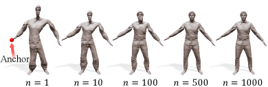
Anchor points
Theoretically, we are able to recover the original mesh from the Laplacian coordinates of vertices by fixing one vertex position as an anchor and solving a linear system (Sorkine et al., 2004). However, in our setting, one anchor may not suffice for reconstructing the accurate final surface , as the Laplacian coordinates are approximate ones predicted by a neural surface Laplacian function , not computed directly from . To improve the accuracy of reconstruction, we set anchor points of a sufficient number as the boundary condition. We select a set of vertex indices as the in Eq. (10) in advance by uniformly sampling (Yuksel, 2015) vertices from the canonical neutral SMPL model , where in our experiments. Figure 6 shows reconstruction results with varying numbers of anchor points.
Reliable anchors
Since anchor points are fixed for solving Eq. (10), they should be as close to the input point cloud as possible. To achieve this property, we set an additional energy term and optimize it along with Eq. (5) when we train the pose-dependent local deformation function :
| (12) |
where measures a vertex-to-point cloud Chamfer distance, is the input point cloud at frame , and is a weight parameter. When the input is a depth map sequence, we apply this term to only visible anchors from the camera viewpoint.
8. Results
8.1. Experiment details
Implementation and training details
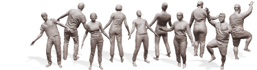
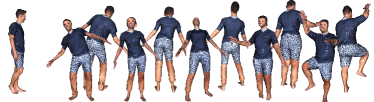
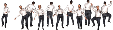
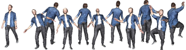
Pose-dependent local deformation function and neural surface Laplacian function are represented as 5- and 3-layer MLPs with ReLU activation, and 600 and 800 feature channels are used per intermediate layer, respectively. In our experiments, we set and . We optimize and with a learning rate of , batch sizes of frames and 5000 points, and 300 and 100 epochs, respectively. The training time is proportional to the numbers of points and frames in the scan data. For instance, the point cloud sequence used for reconstruction in Figure 7 consists of 39k56k points per frame with 200 frames. In that case, it takes about 20 and 30 minutes to train MLPs and , respectively.
Datasets
We evaluate the results of our method qualitatively and quantitatively on single-view and full-body point cloud sequences. We capture RGB-D sequences using an Azure Kinect DK (Kin, 2022) with 1280p resolution for color images and for depth images. Additionally, we use RGB-D sequences that are provided in DSFN (Burov et al., 2021). RGB-D sequences used for experiments contain 200 to 500 frames. We also evaluate our method on full-body point clouds using synthetic datasets: CAFE (Ma et al., 2020), and Resynth (Ma et al., 2021b). We show the reconstruction result from a 2.5D depth point cloud in mint color and the result of a full-body 3D point cloud in olive color.
Timings
In the reconstruction step, for the example in Figure 7, it takes 3ms and 35ms per frame to evaluate the MLPs and , respectively. For solving a sparse linear system to obtain the final detailed mesh that minimizes Eq. (10), it takes 4 seconds for the matrix pre-factorization step and 130ms to obtain the solution for each frame when the mesh contains 113k vertices.
8.2. Analysis
Effect of Laplacian coordinates
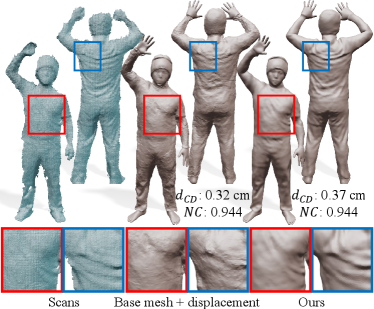
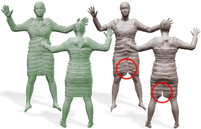
Our approach using Laplacian coordinates preserves local geometric details better than the approach using absolute coordinates of mesh vertices. To verify the claim, we conduct an experiment by changing the neural surface Laplacian function to estimate displacements instead of Laplacian coordinates. We think that this surface function mimics a pose-dependent displacement map. To optimize the surface displacement function, we use the same energy function as Eq. (9) with the change of to the displacement between surface point and scan point . There is no regularization term in Eq. (9), and the maximal capability of the displacement function is exploited for encoding surface details. Nevertheless, the resulting displacement function cannot properly capture structure details, producing rather noisy surfaces (Figure 7 middle). In contrast, our results using Laplacian coordinates are capable of capturing structure details (Figure 7 right) from the input point clouds (Figure 7 left). In Figure 7, we include quantitative results (Chamfer distance and normal consistancy ) on our dataset. The normal consistency is computed using the inner products of the ground truth normals at input points and the normals of the corresponding points on the reconstructed surface. Our result shows a slightly higher Chamfer distance error than the displacement function, but produces more visually pleasing results.
 |
Unclear best weight for smoothness regularization on local deformation
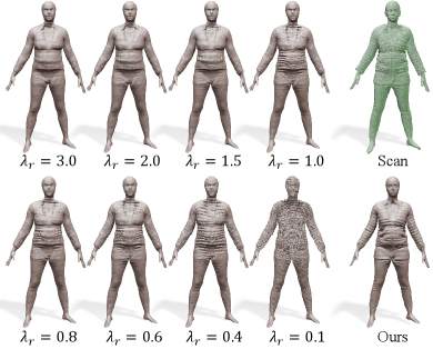
We conduct an experiment that learns the local deformation defined in Sec. 5.2 for a subdivided base mesh that has the same topology as our final mesh. The results (Figure 8 left) show that estimating absolute coordinates is sensitive to the regularization weight defined in Eq. (5). With a large value of , shape details are smoothed out in the reconstructed model. With a small , too small details are reconstructed. Then, it is hard to find the best regularization weight to handle spatially varying structures and sizes of shape details in the input scan (Figure 8 top right). On the contrary, our complete pipeline that learns differential representation performs better without a regularization term (Figure 8 bottom right). Note that all meshes in Figure 8 has the same number of vertices.
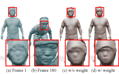
Effect of selective weighting
8.3. Comparisons
We compare our LaplacianFusion with recent representations developed for controllable 3D clothed human reconstruction. The compared representations are based on mesh (Burov et al., 2021), signed distance function (SDF) (Wang et al., 2021), and point cloud (Ma et al., 2021b).
Comparison with DSFN (Mesh)
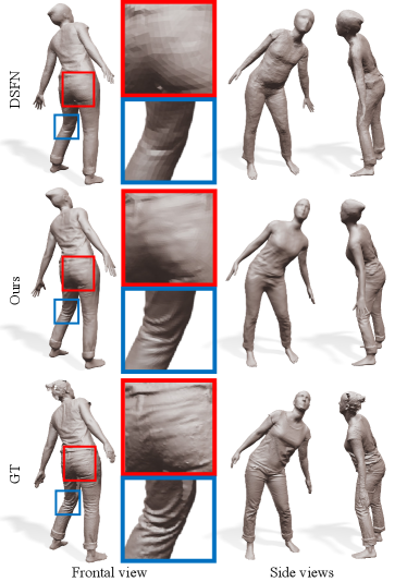
DSFN (Burov et al., 2021) utilizes an explicit mesh to reconstruct a controllable 3D clothed human model from a RGB-D sequence. It represents local details with an offset surface function (dense local deformation), but its spatial regularization smooths out geometric details. Since the source code of DSFN is not published, we compared our results with DSFN on the dataset provided by the authors.
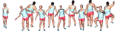
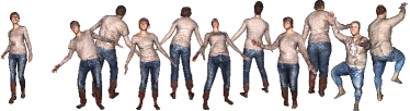
Their real data inputs are captured using an Azure Kinect DK (Kin, 2022) with pix. for color images, and pix. for depth images. Figure 10 shows results on the real dataset provided by DSFN, and our approach produces more plausible details than DSFN. Note that, in this dataset, the captured human stands away from the camera, so input point cloud lacks high-frequency details.
For quantitative evaluation, DSFN uses synthetic pix. RGB-D sequences rendered from BUFF (Zhang et al., 2017), where the camera moves around a subject to cover the whole body. Figure 11 shows the comparison results, and our method preserves the details of the input better. Table 2 shows the measured IOU, chamfer distance (), normal consistency () scores. All three scores of our approach rate better than DSFN.
| Method | IoU | (cm) | |
| DSFN (2021) | 0.832 | 1.56 | 0.917 |
| Ours (same vertex density as DSFN) | 0.863 | 0.99 | 0.933 |
| Ours | 0.871 | 0.94 | 0.941 |
Comparison with MetaAvatar (SDF)
Wang et al. (2021) propose MetaAvatar that represents shape as SDF defined on 3D space. The resulting shape tends to be smoothed due to the limited number of sampling points in the training time. MetaAvatar utilizes the given SMPL parameters for reconstruction, and we use them in the comparison. MetaAvatar evaluates the reconstruction quality using unseen poses with the interpolation capability aspect. Similarly, we sample every 4th frame in the CAPE dataset (Ma et al., 2020) and measure the reconstruction accuracy on every second frame excluding the training frames. The results are shown in Figure 12. In Table 3, we show quantitative results, and the scores of our approach rate better than MetaAvatar.
Comparison with PoP (Point cloud)
Ma et al. (2021b) utilize point cloud representation to deal with topological changes efficiently. We evaluate their method on CAPE dataset in the same configuration used for MetaAvatar in Table 3. In addition, we compare our results with PoP on Resynth dataset (Ma et al., 2021b), which has various cloth types with abundant details. However, Resynth dataset includes human models wearing skirts that cannot be properly handled by our framework (Figure 18), so we do not conduct quantitative evaluation using all subjects. Instead, we select five subjects not wearing skirts to compare our results with PoP quantitatively. We then split the training and test datasets in the same manner as on CAPE dataset.
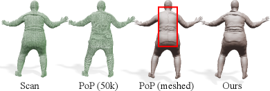
The original implementation of PoP queries the feature tensor with a UV map, resulting in a point cloud with 50k points. Since they are insufficient for representing details on the Resynth dataset, we modified the code to adopt UV map, and obtain 191k points. Table 4 shows quantitative comparisons with the above two settings, and our reconstruction is comparable with the original PoP. Figure 13 presents qualitative results where our mesh is more plausible than the original PoP, and comparable to dense PoP.
In Figure 14, the mesh result obtained from a reconstructed point cloud of PoP contains a vertical line on the back because PoP uses UV coordinates for shape inference. In contrast, our approach can reconstruct clear wrinkles without such artifacts.
| Method | (cm) | ||
| PoP (2021b) | (50k) | 0.43 | 0.970 |
| (153k) | 0.33 | 0.968 | |
| Ours | 0.41 | 0.964 | |
8.4. Applications
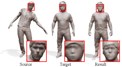
Detail transfer
Our neural surface Laplacian function encodes detailed shape information as the Laplacian coordinates defined at query points in a common domain. As a result, we can easily transfer shape details to other models by evaluating the original surface Laplacian function on the target pose-dependent base mesh. Figure 15 shows an example.
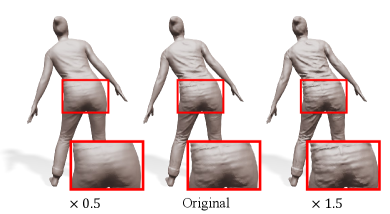
Sharpening & Smoothing
Laplacian coordinates predicted by a neural surface Laplacian function in the Laplacian reconstruction step (Section 7) can be scaled to change the amount of reconstructed shape details. Multiplying a value greater than 1.0 to the predicted Laplacian coordinates performs detail sharpening, and the opposite performs detail smoothing. Figure 15 shows examples.
Animating
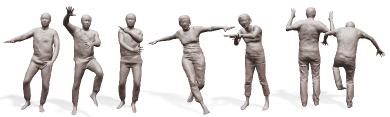
The pose parameters used for evaluating surface functions and can be arbitrary. In the case of reconstructing a scanned animation sequence, we would use the pose parameters estimated from the input scans (Section 5.1). On the other hand, once the functions and have been optimized, any parameters other than can be used to produce unseen poses of the subject. In that case, the validity of shape details of the unseen poses is not guaranteed but our experiments generate reasonable results. In Figure 16, we optimized the functions and on BUFF and CAPE datasets and adopted synthetic motions from AIST++ (Li et al., 2021a). The results show natural variations of shape details depending on the motions.

Texture mapping
In our LaplacianFusion framework, all reconstructed models have the same fixed topology resulting from the subdivision applied to the SMPL model. Then, we can build a common UV parametric domain for texture mapping of any reconstructed model. In Figure 17, we initially transfer a texture from a RenderPoeple model (ren, 2022) to the T-posed canonical neutral SMPL model by using deep virtual markers (Kim et al., 2021). Then, the texture of can be shared with different reconstructed models through the common UV parametric domain.
9. Conclusions
We presented a novel framework, LaplacianFusion, that can reconstruct a detailed and controllable 3D clothed human body model from a 3D point cloud sequence. The key of our framework is Laplacian coordinates that can directly represent local shape variations. We introduce a neural surface Laplacian function that uses Laplacian coordinates for encoding shape details from raw scans and then predicting desirable shape details on a pose-dependent base mesh. The final model is reconstructed by integrating the Laplacian coordinates predicted on a subdivided base mesh. Our approach can also be utilized for other applications, such as detail transfer.
Limitations and future work
Since our framework uses a fixed topology mesh, we cannot cover topological changes, such as opening a zipper. In addition, our base mesh is initialized from a skinned body shape, so it is hard to deal with loose clothes, such as skirts (Figure 18). Our framework relies on registration of the SMPL model to the input scan sequence, and the reconstruction quality is affected by the registration accuracy. Currently, we use simple mid-point subdivision to increase the number of vertices in a base mesh, but a data-driven subdivision approach (Liu et al., 2020) could be considered. Our neural surface Laplacian function is trained for one subject, and generalization of the function to handle other subjects remains as future work. We also plan to generalize our framework for non-human objects.
Acknowledgements.
We would like to thank the anonymous reviewers for their constructive comments. This work was supported by IITP grants (SW Star Lab, 2015-0-00174; AI Innovation Hub, 2021-0-02068; AI Graduate School Program (POSTECH), 2019-0-01906) and KOCCA grant (R2021040136) from Korea government (MSIT and MCST).References
- (1)
- Kin (2022) 2022. Azure Kinect DK – Develop AI Models: Microsoft Azure. https://azure.microsoft.com/en-us/services/kinect-dk/ Online; accessed 19 Jan 2022.
- ren (2022) 2022. Renderpeople-Scanned 3D people models provider. {http://renderpeople.com} Online; accessed 19 Jan 2022.
- Alexa (2003) Marc Alexa. 2003. Differential coordinates for local mesh morphing and deformation. The Visual Computer 19, 2 (2003), 105–114.
- Alldieck et al. (2019) Thiemo Alldieck, Marcus Magnor, Bharat Lal Bhatnagar, Christian Theobalt, and Gerard Pons-Moll. 2019. Learning to reconstruct people in clothing from a single RGB camera. In Proceedings of the IEEE/CVF Conference on Computer Vision and Pattern Recognition (CVPR). 1175–1186.
- Alldieck et al. (2018a) Thiemo Alldieck, Marcus Magnor, Weipeng Xu, Christian Theobalt, and Gerard Pons-Moll. 2018a. Detailed human avatars from monocular video. In Proceedings of the International Conference on 3D Vision (3DV). 98–109.
- Alldieck et al. (2018b) Thiemo Alldieck, Marcus Magnor, Weipeng Xu, Christian Theobalt, and Gerard Pons-Moll. 2018b. Video based reconstruction of 3D people models. In Proceedings of the IEEE/CVF Conference on Computer Vision and Pattern Recognition (CVPR). 8387–8397.
- Alldieck et al. (2021) Thiemo Alldieck, Hongyi Xu, and Cristian Sminchisescu. 2021. imghum: Implicit generative models of 3D human shape and articulated pose. In Proceedings of the IEEE/CVF International Conference on Computer Vision (ICCV). 5461–5470.
- Barrow et al. (1977) Harry G Barrow, Jay M Tenenbaum, Robert C Bolles, and Helen C Wolf. 1977. Parametric correspondence and chamfer matching: Two new techniques for image matching. In Proceedings of International Joint Conference on Artificial Intelligence (IJCAI), Vol. 2. 659–663.
- Bhatnagar et al. (2020) Bharat Lal Bhatnagar, Cristian Sminchisescu, Christian Theobalt, and Gerard Pons-Moll. 2020. Combining Implicit Function Learning and Parametric Models for 3D Human Reconstruction. In Proceedings of the European conference on computer vision (ECCV).
- Bhatnagar et al. (2019) Bharat Lal Bhatnagar, Garvita Tiwari, Christian Theobalt, and Gerard Pons-Moll. 2019. Multi-Garment Net: Learning to Dress 3D People From Images. In Proceedings of the IEEE/CVF International Conference on Computer Vision (ICCV). 5420–5430.
- Burov et al. (2021) Andrei Burov, Matthias Nießner, and Justus Thies. 2021. Dynamic Surface Function Networks for Clothed Human Bodies. In Proceedings of the IEEE/CVF International Conference on Computer Vision (ICCV). 10754–10764.
- Cao et al. (2019) Zhe Cao, Gines Hidalgo, Tomas Simon, Shih-En Wei, and Yaser Sheikh. 2019. OpenPose: realtime multi-person 2D pose estimation using Part Affinity Fields. IEEE Transactions on Pattern Analysis and Machine Intelligence (TPAMI) 43, 1 (2019), 172–186.
- Chen et al. (2021) Xu Chen, Yufeng Zheng, Michael J. Black, Otmar Hilliges, and Andreas Geiger. 2021. SNARF: Differentiable Forward Skinning for Animating Non-Rigid Neural Implicit Shapes. In Proceedings of the IEEE/CVF International Conference on Computer Vision (ICCV). 11594–11604.
- Chen and Zhang (2019) Zhiqin Chen and Hao Zhang. 2019. Learning Implicit Fields for Generative Shape Modeling. In Proceedings of the IEEE/CVF Conference on Computer Vision and Pattern Recognition (CVPR). 5932–5941.
- Chibane et al. (2020) Julian Chibane, Thiemo Alldieck, and Gerard Pons-Moll. 2020. Implicit Functions in Feature Space for 3D Shape Reconstruction and Completion. In Proceedings of the IEEE/CVF Conference on Computer Vision and Pattern Recognition (CVPR). 6970–6981.
- Collet et al. (2015) Alvaro Collet, Ming Chuang, Pat Sweeney, Don Gillett, Dennis Evseev, David Calabrese, Hugues Hoppe, Adam Kirk, and Steve Sullivan. 2015. High-quality streamable free-viewpoint video. ACM Transactions on Graphics (ToG) 34, 4 (2015), 1–13.
- De Aguiar et al. (2010) Edilson De Aguiar, Leonid Sigal, Adrien Treuille, and Jessica K Hodgins. 2010. Stable spaces for real-time clothing. ACM Transactions on Graphics (ToG) 29, 4 (2010), 1–9.
- Deng et al. (2020) Boyang Deng, JP Lewis, Timothy Jeruzalski, Gerard Pons-Moll, Geoffrey Hinton, Mohammad Norouzi, and Andrea Tagliasacchi. 2020. NASA Neural Articulated Shape Approximation. In Proceedings of the European conference on computer vision (ECCV). 612–628.
- Dou et al. (2017) Mingsong Dou, Philip Davidson, Sean Ryan Fanello, Sameh Khamis, Adarsh Kowdle, Christoph Rhemann, Vladimir Tankovich, and Shahram Izadi. 2017. Motion2fusion: Real-time volumetric performance capture. ACM Transactions on Graphics (ToG) 36, 6 (2017), 1–16.
- Dou et al. (2016) Mingsong Dou, Sameh Khamis, Yury Degtyarev, Philip Davidson, Sean Ryan Fanello, Adarsh Kowdle, Sergio Orts Escolano, Christoph Rhemann, David Kim, Jonathan Taylor, Pushmeet Kohli, Vladimir Tankovich, and Shahram Izadi. 2016. Fusion4D: Real-time Performance Capture of Challenging Scenes. ACM Transactions on Graphics (ToG) 35, 4 (2016), 1–13.
- Guan et al. (2012) Peng Guan, Loretta Reiss, David A Hirshberg, Alexander Weiss, and Michael J Black. 2012. Drape: Dressing any person. ACM Transactions on Graphics (ToG) 31, 4 (2012), 1–10.
- Habermann et al. (2020) Marc Habermann, Weipeng Xu, Michael Zollhofer, Gerard Pons-Moll, and Christian Theobalt. 2020. Deepcap: Monocular human performance capture using weak supervision. In Proceedings of the IEEE/CVF Conference on Computer Vision and Pattern Recognition (CVPR). 5052–5063.
- Innmann et al. (2016) Matthias Innmann, Michael Zollhöfer, Matthias Nießner, Christian Theobald, and Marc Stamminger. 2016. Volumedeform: Real-time volumetric non-rigid reconstruction. In Proceedings of the European conference on computer vision (ECCV). 362–379.
- Joo et al. (2018) Hanbyul Joo, Tomas Simon, and Yaser Sheikh. 2018. Total Capture: A 3D Deformation Model for Tracking Faces, Hands, and Bodies. In Proceedings of the IEEE/CVF Conference on Computer Vision and Pattern Recognition (CVPR). 8320–8329.
- Karni and Gotsman (2000) Zachi Karni and Craig Gotsman. 2000. Spectral compression of mesh geometry. In Proceedings of ACM SIGGRAPH conference. 279–286.
- Kazhdan and Hoppe (2013) Michael Kazhdan and Hugues Hoppe. 2013. Screened poisson surface reconstruction. ACM Transactions on Graphics (ToG) 32, 3 (2013), 1–13.
- Kim et al. (2021) Hyomin Kim, Jungeon Kim, Jaewon Kam, Jaesik Park, and Seungyong Lee. 2021. Deep Virtual Markers for Articulated 3D Shapes. In Proceedings of the IEEE/CVF International Conference on Computer Vision (ICCV). 11615–11625.
- Kingma and Ba (2015) Diederik P. Kingma and Jimmy Ba. 2015. Adam: A Method for Stochastic Optimization. In Proceedings of the International Conference on Learning Representations (ICLR), Yoshua Bengio and Yann LeCun (Eds.).
- Lahner et al. (2018) Zorah Lahner, Daniel Cremers, and Tony Tung. 2018. Deepwrinkles: Accurate and realistic clothing modeling. In Proceedings of the European conference on computer vision (ECCV). 667–684.
- Lewis et al. (2000) John P Lewis, Matt Cordner, and Nickson Fong. 2000. Pose space deformation: a unified approach to shape interpolation and skeleton-driven deformation. In Proceedings of ACM SIGGRAPH conference. 165–172.
- Li et al. (2021a) Ruilong Li, Shan Yang, David A. Ross, and Angjoo Kanazawa. 2021a. Learn to Dance with AIST++: Music Conditioned 3D Dance Generation. arXiv:2101.08779 [cs.CV]
- Li et al. (2021b) Zhe Li, Tao Yu, Zerong Zheng, Kaiwen Guo, and Yebin Liu. 2021b. POSEFusion: Pose-guided Selective Fusion for Single-view Human Volumetric Capture. In Proceedings of the IEEE/CVF Conference on Computer Vision and Pattern Recognition (CVPR). 14162–14172.
- Liang et al. (2012) Jian Liang, Rongjie Lai, Tsz Wai Wong, and Hongkai Zhao. 2012. Geometric understanding of point clouds using Laplace-Beltrami operator. In Proceedings of the IEEE/CVF Conference on Computer Vision and Pattern Recognition (CVPR). 214–221.
- Lipman et al. (2004) Yaron Lipman, Olga Sorkine, Daniel Cohen-Or, David Levin, Christian Rossi, and Hans-Peter Seidel. 2004. Differential coordinates for interactive mesh editing. In Proceedings of Shape Modeling International. IEEE, 181–190.
- Liu et al. (2020) Hsueh-Ti Derek Liu, Vladimir G Kim, Siddhartha Chaudhuri, Noam Aigerman, and Alec Jacobson. 2020. Neural subdivision. ACM Transactions on Graphics (ToG) 39, 4 (2020), 124–1.
- Loper et al. (2015) Matthew Loper, Naureen Mahmood, Javier Romero, Gerard Pons-Moll, and Michael J Black. 2015. SMPL: A skinned multi-person linear model. ACM Transactions on Graphics (ToG) 34, 6 (2015), 1–16.
- Ma et al. (2021a) Qianli Ma, Shunsuke Saito, Jinlong Yang, Siyu Tang, and Michael J. Black. 2021a. SCALE: Modeling Clothed Humans with a Surface Codec of Articulated Local Elements. In Proceedings of the IEEE/CVF Conference on Computer Vision and Pattern Recognition (CVPR). 16082–16093.
- Ma et al. (2020) Qianli Ma, Jinlong Yang, Anurag Ranjan, Sergi Pujades, Gerard Pons-Moll, Siyu Tang, and Michael J. Black. 2020. Learning to Dress 3D People in Generative Clothing. In Proceedings of the IEEE/CVF Conference on Computer Vision and Pattern Recognition (CVPR). 6469–6478.
- Ma et al. (2021b) Qianli Ma, Jinlong Yang, Siyu Tang, and Michael J. Black. 2021b. The Power of Points for Modeling Humans in Clothing. In Proceedings of the IEEE/CVF International Conference on Computer Vision (ICCV). 10974–10984.
- Mescheder et al. (2019) Lars Mescheder, Michael Oechsle, Michael Niemeyer, Sebastian Nowozin, and Andreas Geiger. 2019. Occupancy Networks: Learning 3D Reconstruction in Function Space. In Proceedings of the IEEE/CVF Conference on Computer Vision and Pattern Recognition (CVPR). 4460–4470.
- Meyer et al. (2003) Mark Meyer, Mathieu Desbrun, Peter Schröder, and Alan H Barr. 2003. Discrete differential-geometry operators for triangulated 2-manifolds. In Visualization and mathematics III. 35–57.
- Mihajlovic et al. (2021) Marko Mihajlovic, Yan Zhang, Michael J Black, and Siyu Tang. 2021. LEAP: Learning Articulated Occupancy of People. In Proceedings of the IEEE/CVF Conference on Computer Vision and Pattern Recognition (CVPR). 10461–10471.
- Mildenhall et al. (2020) Ben Mildenhall, Pratul P Srinivasan, Matthew Tancik, Jonathan T Barron, Ravi Ramamoorthi, and Ren Ng. 2020. Nerf: Representing scenes as neural radiance fields for view synthesis. In Proceedings of the European conference on computer vision (ECCV). 405–421.
- Newcombe et al. (2015) Richard A. Newcombe, Dieter Fox, and Steven M. Seitz. 2015. DynamicFusion: Reconstruction and tracking of non-rigid scenes in real-time. In Proceedings of the IEEE/CVF Conference on Computer Vision and Pattern Recognition (CVPR). 343–352.
- Palafox et al. (2021) Pablo Palafox, Aljaž Božič, Justus Thies, Matthias Nießner, and Angela Dai. 2021. Npms: Neural parametric models for 3D deformable shapes. In Proceedings of the IEEE/CVF International Conference on Computer Vision (ICCV). 12695–12705.
- Palafox et al. (2022) Pablo Palafox, Nikolaos Sarafianos, Tony Tung, and Angela Dai. 2022. SPAMs: Structured Implicit Parametric Models. In Proceedings of the IEEE/CVF Conference on Computer Vision and Pattern Recognition (CVPR). 12851–12860.
- Park et al. (2019) Jeong Joon Park, Peter Florence, Julian Straub, Richard Newcombe, and Steven Lovegrove. 2019. DeepSDF: Learning Continuous Signed Distance Functions for Shape Representation. In Proceedings of the IEEE/CVF Conference on Computer Vision and Pattern Recognition (CVPR). 165–174.
- Patel et al. (2020) Chaitanya Patel, Zhouyingcheng Liao, and Gerard Pons-Moll. 2020. Tailornet: Predicting clothing in 3D as a function of human pose, shape and garment style. In Proceedings of the IEEE/CVF Conference on Computer Vision and Pattern Recognition (CVPR). 7365–7375.
- Pavlakos et al. (2019) Georgios Pavlakos, Vasileios Choutas, Nima Ghorbani, Timo Bolkart, Ahmed A. A. Osman, Dimitrios Tzionas, and Michael J. Black. 2019. Expressive Body Capture: 3D Hands, Face, and Body from a Single Image. In Proceedings of the IEEE/CVF Conference on Computer Vision and Pattern Recognition (CVPR). 10975–10985.
- Pérez et al. (2003) Patrick Pérez, Michel Gangnet, and Andrew Blake. 2003. Poisson image editing. ACM Transactions on Graphics (ToG) 22, 3 (2003), 313–318.
- Pons-Moll et al. (2017) Gerard Pons-Moll, Sergi Pujades, Sonny Hu, and Michael J Black. 2017. ClothCap: Seamless 4D clothing capture and retargeting. ACM Transactions on Graphics (ToG) 36, 4 (2017), 1–15.
- Romero et al. (2017) Javier Romero, Dimitrios Tzionas, and Michael J. Black. 2017. Embodied Hands: Modeling and Capturing Hands and Bodies Together. ACM Transactions on Graphics (ToG) 36, 6 (2017), 1–17.
- Saito et al. (2019) Shunsuke Saito, Zeng Huang, Ryota Natsume, Shigeo Morishima, Angjoo Kanazawa, and Hao Li. 2019. PIFu: Pixel-Aligned Implicit Function for High-Resolution Clothed Human Digitization. In Proceedings of the IEEE/CVF International Conference on Computer Vision (ICCV). 2304–2314.
- Saito et al. (2020) Shunsuke Saito, Tomas Simon, Jason Saragih, and Hanbyul Joo. 2020. PIFuHD: Multi-Level Pixel-Aligned Implicit Function for High-Resolution 3D Human Digitization. In Proceedings of the IEEE/CVF Conference on Computer Vision and Pattern Recognition (CVPR). 84–93.
- Saito et al. (2021) Shunsuke Saito, Jinlong Yang, Qianli Ma, and Michael J Black. 2021. SCANimate: Weakly supervised learning of skinned clothed avatar networks. In Proceedings of the IEEE/CVF Conference on Computer Vision and Pattern Recognition (CVPR). 2886–2897.
- Santesteban et al. (2019) Igor Santesteban, Miguel A Otaduy, and Dan Casas. 2019. Learning-based animation of clothing for virtual try-on. In Computer Graphics Forum, Vol. 38. 355–366.
- Shao et al. (2022) Ruizhi Shao, Hongwen Zhang, He Zhang, Mingjia Chen, Yan-Pei Cao, Tao Yu, and Yebin Liu. 2022. DoubleField: Bridging the Neural Surface and Radiance Fields for High-Fidelity Human Reconstruction and Rendering. In Proceedings of the IEEE/CVF Conference on Computer Vision and Pattern Recognition (CVPR). 15872–15882.
- Sorkine (2006) Olga Sorkine. 2006. Differential representations for mesh processing. In Computer Graphics Forum, Vol. 25. 789–807.
- Sorkine et al. (2004) Olga Sorkine, Daniel Cohen-Or, Yaron Lipman, Marc Alexa, Christian Rössl, and H-P Seidel. 2004. Laplacian surface editing. In Proceedings of Symposium on Geometry Processing (SGP). 175–184.
- Sorkine et al. (2003) Olga Sorkine, Daniel Cohen-Or, and Sivan Toledo. 2003. High-pass quantization for mesh encoding. In Proceedings of Symposium on Geometry Processing (SGP), Vol. 42. 3.
- Tao et al. (2018) Yu Tao, Zerong Zheng, Kaiwen Guo, Jianhui Zhao, Dai Quionhai, Hao Li, Gerard Pons-Moll, and Yebin Liu. 2018. DoubleFusion: Real-time Capture of Human Performance with Inner Body Shape from a Depth Sensor. In Proceedings of the IEEE/CVF Conference on Computer Vision and Pattern Recognition (CVPR). 7287–7296.
- Tiwari et al. (2020) Garvita Tiwari, Bharat Lal Bhatnagar, Tony Tung, and Gerard Pons-Moll. 2020. SIZER: A Dataset and Model for Parsing 3D Clothing and Learning Size Sensitive 3D Clothing. In Proceedings of the European conference on computer vision (ECCV). 1–18.
- Tiwari et al. (2021) Garvita Tiwari, Nikolaos Sarafianos, Tony Tung, and Gerard Pons-Moll. 2021. Neural-GIF: Neural generalized implicit functions for animating people in clothing. In Proceedings of the IEEE/CVF International Conference on Computer Vision (ICCV). 11708–11718.
- Wang et al. (2021) Shaofei Wang, Marko Mihajlovic, Qianli Ma, Andreas Geiger, and Siyu Tang. 2021. Metaavatar: Learning animatable clothed human models from few depth images. Advances in Neural Information Processing Systems (NeurIPS) 34 (2021), 2810–2822.
- Xiang et al. (2020) Donglai Xiang, Fabian Prada, Chenglei Wu, and Jessica Hodgins. 2020. Monoclothcap: Towards temporally coherent clothing capture from monocular rgb video. In Proceedings of the International Conference on 3D Vision (3DV). 322–332.
- Xu et al. (2020) Hongyi Xu, Eduard Gabriel Bazavan, Andrei Zanfir, William T Freeman, Rahul Sukthankar, and Cristian Sminchisescu. 2020. GHUM & GHUML: Generative 3D Human Shape and Articulated Pose Models. In Proceedings of the IEEE/CVF Conference on Computer Vision and Pattern Recognition (CVPR). 6184–6193.
- Yu et al. (2017) Tao Yu, Kaiwen Guo, Feng Xu, Yuan Dong, Zhaoqi Su, Jianhui Zhao, Jianguo Li, Qionghai Dai, and Yebin Liu. 2017. BodyFusion: Real-time Capture of Human Motion and Surface Geometry Using a Single Depth Camera. In Proceedings of the IEEE/CVF International Conference on Computer Vision (ICCV). 910–919.
- Yu et al. (2021) Tao Yu, Zerong Zheng, Kaiwen Guo, Pengpeng Liu, Qionghai Dai, and Yebin Liu. 2021. Function4D: Real-Time Human Volumetric Capture From Very Sparse Consumer RGBD Sensors. In Proceedings of the IEEE/CVF Conference on Computer Vision and Pattern Recognition (CVPR). 5746–5756.
- Yuksel (2015) Cem Yuksel. 2015. Sample elimination for generating Poisson disk sample sets. In Computer Graphics Forum, Vol. 34. 25–32.
- Zhang et al. (2017) Chao Zhang, Sergi Pujades, Michael J. Black, and Gerard Pons-Moll. 2017. Detailed, Accurate, Human Shape Estimation From Clothed 3D Scan Sequences. In Proceedings of the IEEE/CVF Conference on Computer Vision and Pattern Recognition (CVPR). 4191–4200.