Large deviations and stochastic volatility with jumps:
asymptotic implied volatility for affine models

Antoine Jacquier Institut für Mathematik - Technische Universität Berlin, Germany jacquier@math.tu-berlin.de , Martin Keller-Ressel Institut für Mathematik - Technische Universität Berlin, Germany mkeller@math.tu-berlin.de and Aleksandar Mijatović Department of Statistics, University of Warwick, UK a.mijatovic@warwick.ac.uk

Abstract.

Let $\sigma_{t}(x)$ denote the implied volatility at maturity $t$ for a strike $K=S_{0}\mathrm{e}^{xt}$ , where $x\in\mathbb{R}$ and $S_{0}$ is the current value of the underlying. We show that $\sigma_{t}(x)$ has a uniform (in $x$ ) limit as maturity $t$ tends to infinity, given by the formula $\sigma_{\infty}(x)=\sqrt{2}\left(h^{*}(x)^{1/2}+\left(h^{*}(x)-x\right)^{1/2}\right)$ , for $x$ in some compact neighbourhood of zero in the class of affine stochastic volatility models. The function $h^{*}$ is the convex dual of the limiting cumulant generating function $h$ of the scaled log-spot process. We express $h$ in terms of the functional characteristics of the underlying model. The proof of the limiting formula rests on the large deviation behaviour of the scaled log-spot process as time tends to infinity. We apply our results to obtain the limiting smile for several classes of stochastic volatility models with jumps used in applications (e.g. Heston with state-independent jumps, Bates with state-dependent jumps and Barndorff-Nielsen-Shephard model).

Key words and phrases:

Large deviation principle; Stochastic volatility with jumps; Affine processes; Implied volatility in the large maturity limit

2000 Mathematics Subject Classification:

60G44, 60F10, 91G20

AJ would like to thank MATHEON for financial support.

1. Introduction

Let the process $S=\mathrm{e}^{X}$ model a risky security under an equivalent martingale measure and let $\sigma_{t}(x)$ denote the implied volatility at maturity $t$ for a strike $K=S_{0}\mathrm{e}^{xt}$ (see (53) for the precise definition of $\sigma_{t}(x)$ ). The main result of the present paper (Theorem 14) states that, if the log-spot $X$ follows an affine stochastic volatility process with jumps, then $\sigma_{t}(x)$ converges to $\sigma_{\infty}(x)$ as the maturity $t$ tends to infinity, where $\sigma_{\infty}$ is given by the formula

(1)

\displaystyle\sigma_{\infty}(x)

\displaystyle=

\displaystyle\sqrt{2}\left(h^{*}(x)^{1/2}+\left(h^{*}(x)-x\right)^{1/2}\right).

The function $h$ is the limiting cumulant generating function of the scaled log-spot $(X_{t}/t)_{t\geq 1}$ and $h^{*}$ is its convex dual (i.e. the Fenchel-Legendre transform of $h$ ). Locally uniform convergence of the implied volatility to $\sigma_{\infty}$ is also established.

In [FJ11, FJM11] the limiting behaviour of the smile at large maturities in the Heston model is investigated. Theorem 14 can be viewed as a generalisation of the main result in [FJ11, FJM11]. Not only does it cover a large class of stochastic volatility models with jumps rather than a single affine model with continuous trajectories, but furthermore provides a better understanding of the limit: Theorem 14 states that the limit holds also at the critical points $x^{*}$ and $\widetilde{x}^{*}$ , which are excluded from the analysis in [FJ11, FJM11], and the convergence on the set $\mathbb{R}\setminus\{x^{*},\widetilde{x}^{*}\}$ is shown to be uniform on compact subsets.

In the class of affine stochastic volatility models, the formula for the limiting implied volatility for a fixed strike proved in Tehranchi [Teh09] (see also [Lew00] in the case of the Heston model) also follows from (1), since in Theorem 14 the convergence is uniform on a compact neighbourhood of the origin. In [GL11], the authors give various representations for the implied volatility, including in the large-maturity regime, based on an assumed asymptotic behaviour of certain European derivatives in the underlying model, which is not specified. This representation is not fully explicit in terms of the model parameters and it is therefore unclear how to apply it directly to the class of affine stochastic volatility models.

Contribution of the paper is twofold. First we study the properties of the limiting cumulant generating function $h$ of the affine stochastic volatility models. Results in Lemma 9, Theorem 10 and Corollary 11 give new properties of the function $h$ , which are crucial for the understanding of the large deviation behaviour of the model. Second, the problem of understanding the limiting behaviour of option prices and the corresponding implied volatilities using the large deviation principle is tackled. The uniform limit in $x$ (on all compact subsets of $\mathbb{R}$ ) of vanilla option prices is given in Theorem 13 for non-degenerate affine stochastic volatility models and exponential Lévy models (i.e. degenerate affine stochastic volatility models). As mentioned above Theorem 14 deals with the limiting implied volatility smiles in these classes of models.

Besides giving a formula, which relates model parameters and the limiting implied volatility smile, these theoretical results have the following practical consequences:
(1) in the large-maturity regime studied in this paper, the jumps in the model influence the limiting implied volatility smile as maturity tends to infinity (see examples in 6.1);
(2) for every affine stochastic volatility model there exists an exponential Lévy model such that the smiles of the two models in the limit coincide. In other words the stochasticity of volatility does not (in the affine class) enlarge the family of possible limiting implied volatility smiles (see Section 6 for details).

The starting point of the analysis of the large deviation behaviour of an affine stochastic volatility process $(X,V)$ in the present paper is Theorem 8, taken from [KR11, Theorem 3.4]. This result describes certain properties of the limiting cumulant generating function $h$ , which are however insufficient to understand the essential smoothness of $h$ required in establishing the large deviation principle of $(X_{t}/t)_{t\geq 1}$ . The main contribution of this paper in the area of affine processes is Theorem 10, which identifies sufficient conditions for the process $(X,V)$ that imply essential smoothness of the function $h$ . The conditions in Theorem 10 are easy to apply to the models of interest (see e.g. Section 2.2). Its proof goes beyond the analysis in [KR11] as one is forced to study the special Lévy-Khintchine form of the characteristics of the process, since their general convexity properties no longer suffice to establish the required behaviour of the limit.

The rest of the paper is organized as follows. In Section 2 we define the class of affine stochastic volatility processes and recall some of their properties. In Section 3 we review briefly basic concepts in the theory of large deviations and state the Gärtner-Ellis theorem. Section 4 establishes the large deviations principle for the scaled log-stock of an affine stochastic volatility model as maturity tends to infinity. Sections 5 and 6 respectively translate this result into option price and implied volatility asymptotics. Numerical examples are given at the end of Section 6.

2. Affine stochastic volatility models with jumps

Consider a stochastic model for a risky security $S=(S_{t})_{t\geq 0}$ given by

(2)

\displaystyle S_{t}

\displaystyle=

\displaystyle\exp((r-d)t+X_{t}),\quad t\geq 0\;,

where the interest rate $r$ and the dividend yield $d$ are non-negative and constant and the log-price process $X=(X_{t})_{t\geq 0}$ starts at $X_{0}\in\mathbb{R}$ . Since the dynamics of $S$ is given under a risk-neutral measure, the forward price process is $(\exp(X_{t}))_{t\geq 0}$ . We assume throughout the paper without loss of generality that $S$ is a forward price process (i.e. $r=d$ ). Denote by $V=(V_{t})_{t\geq 0}$ a process, starting at a constant level $V_{0}>0$ . The process $V$ can be interpreted as the instantaneous variance process of $X$ but may also control the arrival rate of jumps of $X$ . We make the following assumptions on the process $(X,V)$ throughout the paper.

A1:

$(X,V)$ is a stochastically continuous, time-homogeneous Markov process with state-space $D=\mathbb{R}\times\mathbb{R}_{\geqslant 0}$ , where $\mathbb{R}_{\geqslant 0}:=[0,\infty)$ .

A2:

The cumulant generating function $\Phi_{t}(u,w)$ of $(X_{t},V_{t})$ is of a particular affine form: there exist functions $\phi(t,u,w)$ and $\psi(t,u,w)$ such that

	$\displaystyle\Phi_{t}(u,w)$	$\displaystyle:=$	$\displaystyle\log\mathsf{E}\left[\left.\exp(uX_{t}+wV_{t})\right\|X_{0},V_{0}\right]$
		$\displaystyle=$	$\displaystyle\phi(t,u,w)+V_{0}\psi(t,u,w)+X_{0}u$

for all $(t,u,w)\in\mathbb{R}_{\geqslant 0}\times\mathbb{C}^{2}$ , where the expectation exists.

Remarks.

(i) A1 and A2 make $(X,V)$ into an affine process in the sense of [DFS03].

(ii) A1 and A2 imply a homogeneity property of $(X,V)$ : if the starting value $(X_{0},V_{0})$ is shifted by $(x,0)\in D$ , the law of the random variable $(X_{t},V_{t})$ is shifted by the vector $(x,0)$ for any $t\geq 0$ .

(iii) Assumptions A1 and A2 imply that the variance process $V$ is a one-dimensional strong Markov process in its own right.

(iv) The law of iterated expectations applied to $\Phi_{t}(u,w)$ yields the flow-equations for $\phi$ and $\psi$ (see [DFS03, Eq. (3.8)–(3.9)]):

(3)

\begin{split}\phi(t+s,u,w)&=\phi(t,u,w)+\phi(s,u,\psi(t,u,w)),\\ \psi(t+s,u,w)&=\psi(s,u,\psi(t,u,w)),\end{split}

for all $t,s\geq 0$ .

(v) It is shown in [KR11, Thm. 2.1] (see also [DFS03]) that if $|\phi(\tau,u,\eta)|,|\psi(\tau,u,\eta)|<\infty$ for $(\tau,u,\eta)\in(0,\infty)\times\mathbb{C}^{2}$ , then for all $t\in[0,\tau)$ and $w\in\mathbb{C}$ such that $\Re\,w\leq\Re\,\eta$ , the functions $\phi$ and $\psi$ satisfy the generalized Riccati equations


(4a)	$\displaystyle\partial_{t}\phi(t,u,w)$	$\displaystyle=F(u,\psi(t,u,w)),\quad\phi(0,u,w)=0,$
(4b)	$\displaystyle\partial_{t}\psi(t,u,w)$	$\displaystyle=R(u,\psi(t,u,w)),\quad\psi(0,u,w)=w,$

where

(5)

F(u,w):=\left.\frac{\partial}{\partial t}\phi(t,u,w)\right|_{t=0+},\qquad R(u,w):=\left.\frac{\partial}{\partial t}\psi(t,u,w)\right|_{t=0+}.

Furthermore for all $t\in[0,\tau]$ we have $|\phi(t,u,w)|,|\psi(t,u,w)|<\infty$ .

(vi) If $(X,V)$ is a diffusion process, then ODEs (4) become classical Riccati. Note also that (4) follows from the flow equations (3) by differentiation with respect to $s$ .

(vii) $\phi$ and $\psi$ can for small $t$ be expressed implicitly in terms of $F$ and $R$ as

\phi(t,u,w)=\int_{0}^{t}{F(u,\psi(s,u,w))\;\mathrm{d}s}\qquad\text{and}\qquad\int_{w}^{\psi(t,u,w)}{\frac{\mathrm{d}\eta}{R(u,\eta)}}=t\;.

The functions $F$ and $R$ , defined in (5), must be of Lévy-Khintchine form (see [DFS03]). In other words


(6a)	$\displaystyle F(u,w)$	$\displaystyle=\left\langle\frac{a}{2}(u,w)^{\prime},(u,w)^{\prime}\right\rangle+\left\langle b,(u,w)^{\prime}\right\rangle-c$
	$\displaystyle+\int_{D\setminus\{0\}}{\left(\mathrm{e}^{\langle\xi,(u,w)^{\prime}\rangle}-1-\langle\omega_{F}(\xi),(u,w)^{\prime}\rangle\right)\,m(\mathrm{d}\xi)},$
(6b)	$\displaystyle R(u,w)$	$\displaystyle=\left\langle\frac{\alpha}{2}(u,w)^{\prime},(u,w)^{\prime}\right\rangle+\left\langle\beta,(u,w)^{\prime}\right\rangle-\gamma$
	$\displaystyle+\int_{D\setminus\{0\}}{\left(\mathrm{e}^{\langle\xi,(u,w)^{\prime}\rangle}-1-\langle\omega_{R}(\xi),(u,w)^{\prime}\rangle\right)\,\mu(\mathrm{d}\xi)},$

where $D=\mathbb{R}\times\mathbb{R}_{\geqslant 0}$ , $\langle\cdot,\cdot\rangle$ is the inner product on $\mathbb{R}^{2}$ , $(u,w)^{\prime}$ denotes transposition, $\omega_{F}$ , $\omega_{R}$ are suitable truncation functions, which we fix by defining

\omega_{F}(\xi)=\left(\begin{array}[]{@{}c@{}}\frac{\xi_{1}}{1+\xi_{1}^{2}}\\ 0\end{array}\right)\qquad\text{and}\qquad\omega_{R}(\xi)=\left(\begin{array}[]{@{}c@{}}\frac{\xi_{1}}{1+\xi_{1}^{2}}\\ \frac{\xi_{2}}{1+\xi_{2}^{2}}\end{array}\right),\quad\text{where}\quad\xi=\left(\begin{array}[]{@{}c@{}}\xi_{1}\\ \xi_{2}\end{array}\right),

and the parameters $(a,\alpha,b,\beta,m,\mu)$ satisfy the following admissibility conditions:

•

$a,\alpha$ are positive semi-definite $2\times 2$ -matrices with $a_{12}=a_{21}=a_{22}=0$ ;
•

$b\in D$ , $\beta\in\mathbb{R}^{2}$ and $c,\gamma\in\mathbb{R}_{\geqslant 0}$ ;
•

$m$ and $\mu$ are Lévy measures on $D$ and $\int_{D\setminus\{0\}}{\left((\xi_{1}^{2}+\xi_{2})\wedge 1\right)\,m(\mathrm{d}\xi)}<\infty$ .

Assumptions A1 and A2, the generalized Riccati equations and the Lévy-Khintchine decomposition (6) lead to the following interpretation of $F$ and $R$ : $F$ characterizes the state-independent dynamics of the process $(X,V)$ while $R$ characterizes its state-dependent dynamics. The instantaneous characteristics of the Markov process $(X,V)$ are given as follows: $a+V\alpha$ the instantaneous covariance matrix, $b+V\beta$ the instantaneous drift, $m(\mathrm{d}\xi)+V\mu(\mathrm{d}\xi)$ the instantaneous arrival rate of jumps with jump heights in $\mathrm{d}\xi$ and $c+\gamma V$ the instantaneous killing rate.

The function $\chi$ defined below plays a key role in the characterisation of the martingale property of the process $S=\exp(X)$ .

Definition 1.

For each $u\in\mathbb{R}$ such that $R(u,0)<\infty$ , define $\chi(u)$ as

\chi(u):=\left.\partial_{2}R(u,w)\right|_{w=0}:=\left.\frac{\partial R}{\partial w}(u,w)\right|_{w=0}\;.

Remarks.

(i) The condition $R(u,0)<\infty$ implies that, for some $\delta>0$ the function $w\mapsto R(u,w)$ is convex on $(-\delta,0]$ and differentiable on $(-\delta,0)$ , since the process $V$ does not have negative jumps. Therefore $\chi(u)$ is a well-defined, possibly equal to $+\infty$ , convex function given by the limit of $\partial_{2}R(u,w)$ as $w\uparrow 0$ . It can be expressed explicitly as

\chi(u)=\alpha_{12}u+\beta_{1}+\int_{D\setminus\{0\}}{\xi_{2}\left(\mathrm{e}^{u\xi_{1}}-\frac{1}{1+\xi_{2}^{2}}\right)\,\mu(\mathrm{d}\xi)},\qquad\text{where}\quad\xi^{\prime}=(\xi_{1},\xi_{2})\;.

(ii) The sufficient and necessary condition for $S$ to be conservative and a martingale, in terms of $R,F$ and $\chi$ , is given in [KR11, Thm. 2.5]. A simple sufficient condition for these properties reads (see [KR11, Cor. 2.7]):

$\bullet$

if $F(0,0)=R(0,0)=0$ and $\chi(0)<\infty$ then $S=\exp(X)$ is conservative.
$\bullet$

if $S$ is conservative, $F(1,0)=R(1,0)=0$ and $\chi(1)<\infty$ , then $S=\exp(X)$ is a martingale.

Since $S$ serves as a forward price process under a risk-neutral measure $\mathsf{P}$ in an arbitrage-free asset pricing model, it has to be conservative and a martingale and hence we assume:

A3:: $F(0,0)=R(0,0)=F(1,0)=R(1,0)=0$ and $\chi(0)+\chi(1)<\infty$ .

In particular $F(0,0)=R(0,0)=0$ in assumption A3 means that the instantaneous killing rates $c$ and $\gamma$ in (6) are zero and the condition $F(1,0)=R(1,0)=0$ is closely related to the functions $\psi(\cdot,1,0)$ and $\phi(\cdot,1,0)$ being identically equal to zero (see the generalized Riccati equations in (4)), which implies the martingale property of $S=\exp(X)$ . The following non-degeneracy assumption will guarantee the stochasticity of volatility of the process $X$ .

A4:: There exists some $u\in\mathbb{R}$ , such that $R(u,0)\neq 0$ .

Definition 2.

The process $(X,V)$ is a non-degenerate (resp. degenerate) affine stochastic volatility process if it satisfies assumptions A1 – A4 (resp. A1 – A3 and does not satisfy A4) and $S=\mathrm{e}^{X}$ is the corresponding affine stochastic volatility model.

Remark.

Assumption A4 excludes the degenerate case where the distribution of $X$ does not depend on the volatility state $V_{0}$ . Indeed, if A4 is not satisfied, i.e. $R(\cdot,0)\equiv 0$ , then (4) implies that $\psi(t,u,0)=0$ and $\phi(t,u,0)=tF(u,0)$ for all $(t,u)\in\mathbb{R}_{\geqslant 0}\times\mathbb{C}$ where the expectation in assumption A2 exists. Hence if A4 does not hold, then A2, (6a) and the characterisation theorem for regular affine processes [DFS03, Theorem 2.7] imply that $S=\mathrm{e}^{X}$ is an exponential Lévy model. In particular the class of affine stochastic volatility models includes the Black-Scholes model as a degenerate case.

The following proposition describes certain properties of $F$ and $R$ that will play a crucial role in Section 4.1.

Proposition 3.

Let $(X,V)$ be a non-degenerate affine stochastic volatility model and let the sets $\mathcal{D}_{F}=\left\{(u,w)\in\mathbb{R}^{2}:F(u,w)<\infty\right\}$ and $\mathcal{D}_{R}=\left\{(u,w)\in\mathbb{R}^{2}:R(u,w)<\infty\right\}$ be the effective domains of the functions $F$ and $R$ respectively. Then the following holds:

(A)

$F$ and $R$ are lower semicontinuous convex functions, which are continuously differentiable in the interiors $\mathcal{D}_{F}^{\circ}$ and $\mathcal{D}_{R}^{\circ}$ (in $\mathbb{R}^{2}$ ), and their effective domains $\mathcal{D}_{F}$ and $\mathcal{D}_{R}$ are also convex;
(B)

$F$ and $R$ are either affine or strictly convex functions when restricted to one-dimensional affine subspaces of $\mathbb{R}^{2}$ .

Proof.

The Lévy-Khintchine representation for $F$ and $R$ in (6) implies that they are cumulant generating functions of some (infinitely divisible) random vectors taking values in $\mathbb{R}^{2}$ . Hölder’s inequality yields that $F$ and $R$ are convex. The dominated convergence theorem and the representation in (6) implies that $F$ and $R$ are analytic in $\mathcal{D}_{F}^{\circ}$ and $\mathcal{D}_{R}^{\circ}$ respectively. Fatou’s lemma implies that the functions $F$ and $R$ are lower semicontinuous. Since $F$ and $R$ are cumulant generating functions, the second derivative of their restriction to an affine subspace is either identically zero or strictly positive everywhere (each affine subspace in $\mathbb{R}^{2}$ corresponds to a random variable which takes values in $\mathbb{R}$ and may or may not be constant almost surely). This concludes the proof. ∎

2.1. SDE representation of affine stochastic volatility processes

In order to define an affine stochastic volatility model one needs to choose admissible parameters $(a,\alpha,b,\beta,m,\mu)$ such that the corresponding process $(X,V)$ , which exists by [DFS03, Thm. 2.7], satisfies assumptions A1 – A3 (note that $c=\gamma=0$ by A3 and will henceforth be ignored). This procedure yields a semigroup, and hence the law, of the Markov process $(X,V)$ which is in principle sufficient for option pricing. However path-wise descriptions of the pricing models in financial markets are widely used as they add to the intuitive understanding of the properties of the model. In the rest of this section we briefly describe a path-wise construction of the process $(X,V)$ , given in [DL06], and relate it to the most popular affine stochastic volatility models used in derivatives pricing.

Assume that the parameters $(a,\alpha,b,\beta,m,\mu)$ are admissible and suppose in addition that the tails (i.e. the large jumps) of $m$ and $\mu$ satisfy:

(7)

\displaystyle\int_{\|\xi\|>1}{\|\xi\|\,m(\mathrm{d}\xi)}<\infty\qquad\text{and}\qquad\int_{\|\xi\|>1}{\|\xi\|\,\mu(\mathrm{d}\xi)}<\infty

where $\|\xi\|=\langle\xi,\xi\rangle.$ Let

(8)

\begin{split}\widetilde{b}_{1}&=b_{1}+\int_{D\setminus\{0\}}\frac{\xi_{1}^{3}}{1+\xi_{1}^{2}}\,m(\mathrm{d}\xi),\quad\widetilde{b}_{2}=b_{2},\\ \widetilde{\beta}_{i}&=\beta_{i}+\int_{D\setminus\{0\}}\frac{\xi_{i}^{3}}{1+\xi_{i}^{2}}\,\mu(\mathrm{d}\xi)\quad\text{for}\quad i=1,2.\end{split}

Note that the integrals in (8) are finite by (7) and the parameters $(a,\alpha,\widetilde{b},\widetilde{\beta},m,\mu)$ are admissible with appropriate truncation functions.

Let $(\Omega,\mathcal{F},(\mathcal{F}_{t})_{t\geq 0},\mathsf{P})$ be a filtered probability space equipped with

$\bullet$

a three-dimensional standard Brownian motion $(B^{0},B^{1},B^{2})$ ,
$\bullet$

a Poisson random measure $N_{0}(\mathrm{d}s,\mathrm{d}\xi)$ on $\mathbb{R}_{\geqslant 0}\times D$ with compensator $\mathrm{d}s\,m(\mathrm{d}\xi)$ ,
$\bullet$

a Poisson random measure $N_{1}(\mathrm{d}s,\mathrm{d}u,\mathrm{d}\xi)$ on $\mathbb{R}_{\geqslant 0}^{2}\times D$ with compensator $\mathrm{d}s\,\mathrm{d}u\,\mu(\mathrm{d}\xi)$ ,

where as usual $D=\mathbb{R}\times\mathbb{R}_{\geqslant 0}$ denotes the state-space of the model. Let

\widetilde{N}_{0}(\mathrm{d}s,\mathrm{d}\xi)=N_{0}(\mathrm{d}s,\mathrm{d}\xi)-\mathrm{d}s\,m(\mathrm{d}\xi)\quad\text{and}\quad\widetilde{N}_{1}(\mathrm{d}s,\mathrm{d}u,\mathrm{d}\xi)=N_{1}(\mathrm{d}s,\mathrm{d}u,\mathrm{d}\xi)-\mathrm{d}s\,\mathrm{d}u\,\mu(\mathrm{d}\xi)

be the compensated Poisson random measures and let $\sigma$ be a $2\times 2$ -matrix such that $\sigma\sigma^{\top}=\alpha$ . Theorem 6.2 in [DL06] implies that the system of SDEs

$\displaystyle\mathrm{d}X_{t}$	$\displaystyle=$	$\displaystyle\left(\widetilde{b}_{1}+V_{t}\widetilde{\beta}_{1}\right)\mathrm{d}t+\sqrt{a_{11}}\mathrm{d}B_{t}^{0}+\sqrt{V_{t}}\sigma_{11}\mathrm{d}B_{t}^{1}+\sqrt{V_{t}}\sigma_{12}\mathrm{d}B_{t}^{2}+$
		$\displaystyle\int_{D\setminus\{0\}}\xi_{1}\widetilde{N}_{0}(\mathrm{d}t,\mathrm{d}\xi)+\int_{D\setminus\{0\}}\int_{0}^{V_{t-}}\xi_{1}\widetilde{N}_{1}(\mathrm{d}t,\mathrm{d}u,\mathrm{d}\xi),$
$\displaystyle\mathrm{d}V_{t}$	$\displaystyle=$	$\displaystyle\left(\widetilde{b}_{2}+V_{t}\widetilde{\beta}_{2}\right)\mathrm{d}t+\sqrt{V_{t}}\sigma_{21}\mathrm{d}B_{t}^{1}+\sqrt{V_{t}}\sigma_{22}\mathrm{d}B_{t}^{2}+$
		$\displaystyle\int_{D\setminus\{0\}}\xi_{2}N_{0}(\mathrm{d}t,\mathrm{d}\xi)+\int_{D\setminus\{0\}}\int_{0}^{V_{t-}}\xi_{2}\widetilde{N}_{1}(\mathrm{d}t,\mathrm{d}u,\mathrm{d}\xi),$

with initial condition $(X_{0},V_{0})\in\mathbb{R}\times(0,\infty)$ , has a unique strong solution $(X,V)$ that is an affine Markov process with admissible parameters $(a,\alpha,b,\beta,m,\mu)$ .

Remarks.

(i) The change of parameters $b$ and $\beta$ introduced in (8) is inessential. Its function is to establish the notational compatibility with [DL06].

(ii) The integrals in (2.1)–(2.1) against $\widetilde{N}_{1}$ are taken over a random set whose $\mathrm{d}s\,\mathrm{d}u\,\mu(\mathrm{d}\xi)$ -volume is proportional to $V_{t-}$ . This, together with the structure of the Poisson random measure $N_{1}$ , reinforces the intuition that the jumps of the process $(X,V)$ that correspond to the integral term with respect to $\widetilde{N}_{1}$ have random intensity which is proportional to $V$ .

2.2. Examples of affine stochastic volatility models

We now describe some of the affine stochastic volatility models that are of interest in the financial markets and can be obtained as solutions of the special cases of SDE (2.1)–(2.1).

2.2.1. Heston model

The log-price $X$ and the stochastic variance process $V$ are given under the risk-neutral measure by the SDE

	$\displaystyle\mathrm{d}X_{t}$	$\displaystyle=-\frac{V_{t}}{2}\,\mathrm{d}t+\sqrt{V_{t}}\,\mathrm{d}W^{1}_{t},$
	$\displaystyle\mathrm{d}V_{t}$	$\displaystyle=-\lambda(V_{t}-\theta)\,\mathrm{d}t+\zeta\sqrt{V_{t}}\,\mathrm{d}W^{2}_{t},\,$

where $W^{1},W^{2}$ are Brownian motions with correlation parameter $\rho\in(-1,1)$ , and $\zeta,\lambda,\theta>0$ (see [Hes93]). The affine characteristics of the model are


(11a)	$\displaystyle F(u,w)$	$\displaystyle=\lambda\theta w,$
(11b)	$\displaystyle R(u,w)$	$\displaystyle=\frac{1}{2}(u^{2}-u)+\frac{\zeta^{2}}{2}w^{2}-\lambda w+uw\rho\zeta.$

It is easily seen that $\chi$ is given by

(12)

\chi(u)=\rho\zeta u-\lambda

and it is trivial to check that A1 – A4 are satisfied.

2.2.2. Heston model with state-independent jumps

Let $J$ be a pure-jump Lévy process independent of the correlated Brownian motions $W^{1}$ and $W^{2}$ . The Heston-with-jumps model is defined by the SDEs

	$\displaystyle\mathrm{d}X_{t}$	$\displaystyle=\left(\delta-\frac{V_{t}}{2}\right)\,\mathrm{d}t+\sqrt{V_{t}}\,\mathrm{d}W^{1}_{t}+\mathrm{d}J_{t},$
	$\displaystyle\mathrm{d}V_{t}$	$\displaystyle=-\lambda(V_{t}-\theta)\,\mathrm{d}t+\zeta\sqrt{V_{t}}\,\mathrm{d}W^{2}_{t},$

where $\zeta,\lambda,\theta>0$ and $\delta\in\mathbb{R}$ . Assume that $J$ is a spectrally negative Lévy process with characteristic exponent $\frac{1}{t}\log\mathsf{E}[\mathrm{e}^{uJ_{t}}]=\int_{(-\infty,0)}(\mathrm{e}^{u\xi_{1}}-1-u\xi_{1}/(1+\xi_{1}^{2}))\,\nu(\mathrm{d}\xi_{1})$ . Since $J$ only jumps down, this captures the generic situation in the modelling of equity markets. Assume further that the jumps of $J$ are integrable (i.e. $\int_{(-\infty,0)}|\xi_{1}|\,\nu(\mathrm{d}\xi_{1})<\infty$ ). In order to identify the coefficients in (2.1)–(2.1), we compensate $J$ so that it becomes a martingale and can hence be expressed as an integral against the compensated Poisson random measure $\widetilde{N}_{0}$ . This implies

\widetilde{b}_{1}=\delta+\int_{(-\infty,0)}\frac{\xi_{1}^{3}}{1+\xi_{1}^{2}}\,\nu(\mathrm{d}\xi_{1}).

It is easily seen that $a=0$ , $\alpha_{11}=1$ , $\alpha_{12}=\rho\zeta$ , $\alpha_{22}=\zeta^{2}$ , $\mu\equiv 0$ and $m(\mathrm{d}\xi)=(\nu\otimes\delta_{0})(\mathrm{d}\xi)$ , where $\delta_{0}$ is the Dirac delta measure. Therefore $b_{1}=\delta$ , $b_{2}=\lambda\theta$ , $\beta_{1}=-1/2$ and $\beta_{2}=-\lambda$ . The martingale condition ( $F(1,0)=0$ ) implies $\delta=-\int_{(-\infty,0)}\left(\mathrm{e}^{\xi_{1}}-1-\xi_{1}/(1+\xi_{1}^{2})\right)\,\nu(\mathrm{d}\xi_{1})$ and the affine form of the model is given by


(13a)	$\displaystyle F(u,w)$	$\displaystyle=\lambda\theta w+\widetilde{\kappa}(u),$
(13b)	$\displaystyle R(u,w)$	$\displaystyle=\frac{1}{2}(u^{2}-u)+\frac{\zeta^{2}}{2}w^{2}-\lambda w+uw\rho\zeta,$

where $\widetilde{\kappa}(u)$ is the compensated cumulant generating function of the jump part, i.e.

(14)

\widetilde{\kappa}(u)=\int_{(-\infty,0)}\left(\mathrm{e}^{\xi_{1}u}-1-u\left(\mathrm{e}^{\xi_{1}}-1\right)\right)\,\nu(\mathrm{d}\xi_{1}).

2.2.3. A model of Bates with state-dependent jumps

We consider the model given by

	$\displaystyle\mathrm{d}X_{t}$	$\displaystyle=-\left(\frac{1}{2}+\delta\right)V_{t}\,\mathrm{d}t+\sqrt{V_{t}}\,\mathrm{d}W^{1}_{t}+\int_{\mathbb{R}\setminus\{0\}}{\xi_{1}\,\widetilde{N}(V_{t},\mathrm{d}t,\mathrm{d}\xi_{1})},$
	$\displaystyle\mathrm{d}V_{t}$	$\displaystyle=-\lambda(V_{t}-\theta)\,\mathrm{d}t+\zeta\sqrt{V_{t}}\,\mathrm{d}W^{2}_{t},$

where as before $\lambda,\theta,\zeta>0$ , $\delta\in\mathbb{R}$ and the Brownian motions $W^{1}$ and $W^{2}$ are correlated with correlation $\rho\in(-1,1)$ . The jump component is given by $\widetilde{N}(V_{t},\mathrm{d}t,\mathrm{d}\xi_{1})=N(V_{t},\mathrm{d}t,\mathrm{d}\xi_{1})-n(V_{t},\mathrm{d}t,\mathrm{d}\xi_{1})$ , where $N(V_{t},\mathrm{d}t,\mathrm{d}\xi_{1})$ is a Poisson random measure independent of $W^{1}$ and $W^{2}$ with intensity measure $n(V_{t},\mathrm{d}t,\mathrm{d}\xi_{1})$ of the state-dependent form $V_{t}\nu(\mathrm{d}\xi_{1})\mathrm{d}t$ . Here $\nu(\mathrm{d}\xi_{1})$ denotes a Lévy measure on $\mathbb{R}\setminus\{0\}$ . A model of this kind has been proposed in [Bat00] to explain the time-variation of jump-risk implicit in observed option prices.

As in Section 2.2.2, we assume that the support of $\nu(\mathrm{d}\xi_{1})$ is contained in $(-\infty,0)$ and that the inequality $\int_{(-\infty,0)}|\xi_{1}|\,\nu(\mathrm{d}\xi_{1})<\infty$ is satisfied. We can identify the parameters in (2.1)–(2.1) as $a=0$ , $\alpha_{11}=1$ , $\alpha_{12}=\rho\zeta$ , $\alpha_{22}=\zeta^{2}$ , $\widetilde{\beta}_{1}=-1/2-\delta$ , $\widetilde{\beta}_{2}=-\lambda$ , $\widetilde{b}_{1}=0$ , $\widetilde{b}_{2}=b_{2}=\lambda\theta$ , $m\equiv 0$ and $\mu(\mathrm{d}\xi)=(\nu\otimes\delta_{0})(\mathrm{d}\xi)$ , where $\delta_{0}$ is the Dirac delta concentrated at $0$ . Hence we find

\beta_{1}=-\frac{1}{2}-\delta-\int_{(-\infty,0)}\frac{\xi_{1}^{3}}{1+\xi_{1}^{2}}\,\nu(\mathrm{d}\xi_{1})

and $\beta_{2}=-\lambda$ , $b_{1}=0$ . The functions $F$ and $R$ for the Bates model are


(15a)	$\displaystyle F(u,w)$	$\displaystyle=\lambda\theta w,$
(15b)	$\displaystyle R(u,w)$	$\displaystyle=\frac{1}{2}(u^{2}-u)+\frac{\zeta^{2}}{2}w^{2}-\lambda w+uw\rho\zeta+\widetilde{\kappa}(u),$

where $\widetilde{\kappa}(u)=\int_{(-\infty,0)}\left(\mathrm{e}^{\xi_{1}u}-1-u\left(\mathrm{e}^{\xi_{1}}-1\right)\right)\,\nu(\mathrm{d}\xi_{1})$ and the martingale property ( $R(1,0)=0$ ) was used to determine the value of the parameter $\delta=\int_{(-\infty,0)}\left(\mathrm{e}^{\xi_{1}}-1-\xi_{1}\right)\,\nu(\mathrm{d}\xi_{1})$ . It is clear that $\chi(u)=\rho\zeta u-\lambda$ and that A1 – A4 are satisfied.

2.2.4. The Barndorff-Nielsen-Shephard (BNS) model

The BNS model was introduced in [BNS01] as a model for asset pricing. Under a risk-neutral measure, it can be defined by the following SDE

	$\displaystyle\mathrm{d}X_{t}$	$\displaystyle=(\delta-\frac{1}{2}V_{t})\mathrm{d}t+\sqrt{V_{t}}\,\mathrm{d}W_{t}+\rho\,\mathrm{d}J_{\lambda t},$
	$\displaystyle\mathrm{d}V_{t}$	$\displaystyle=-\lambda V_{t}\,\mathrm{d}t+\mathrm{d}J_{\lambda t},$

where $\lambda>0$ , $\rho<0$ and $(J_{t})_{t\geq 0}$ is a Lévy subordinator with the Lévy measure $\nu$ , i.e. a pure jump Lévy process that increases a.s. The cumulant generating function $\kappa(u)$ of $(J_{t})_{t\geq 0}$ takes the form

(16)

\displaystyle\kappa(u)=\int_{(0,\infty)}(\mathrm{e}^{u\xi_{2}}-1)\,\nu(\mathrm{d}\xi_{2}).

To conform with (7) we further assume that $\int_{(0,\infty)}\xi_{2}\,\nu(\mathrm{d}\xi_{2})<\infty$ . The drift $\delta$ will be determined by the martingale condition for $S$ . The time-scaling $J_{\lambda t}$ is introduced in [BNS01] to make the invariant distribution of the variance process independent of $\lambda$ . The distinctive features of the BNS model are that the variance process has no diffusion component, i.e. moves purely by jumps, and the negative correlation between variance and price movements is achieved by simultaneous jumps in $V$ and $X$ .

It follows from (2.1)–(2.1) and the SDE above that $a=\alpha_{12}=\alpha_{22}=0$ , $\alpha_{11}=1$ , $\mu\equiv 0$ and

m(\mathrm{d}\xi)=I_{\{\xi_{1}=\rho\xi_{2}\}}\lambda\nu(\mathrm{d}\xi_{2}),

where $I_{\{\xi_{1}=\rho\xi_{2}\}}$ denotes the indicator function of the half-line $\xi_{1}=\rho\xi_{2}$ in $D\setminus\{0\}$ . Therefore it follows that $\widetilde{\beta}_{1}=\beta_{1}=-1/2$ , $\widetilde{\beta}_{2}=\beta_{2}=-\lambda$ , $\widetilde{b}_{2}=b_{2}=0$ , $\widetilde{b}_{1}=\delta+\lambda\int_{(0,\infty)}\rho\xi_{2}\,\nu(\mathrm{d}\xi_{2})$ and

b_{1}=\delta+\lambda\int_{(0,\infty)}\frac{\rho\xi_{2}}{1+(\rho\xi_{2})^{2}}\,\nu(\mathrm{d}\xi_{2}).

The definition of $F$ in (6) and the martingale condition $F(1,0)=0$ imply that we need to define $\delta=-\lambda\kappa(\rho)$ , where $\kappa$ is the cumulant generating function of $J$ given in (16). The BNS model is an affine stochastic volatility model with $F$ and $R$ given by


(17a)	$\displaystyle F(u,w)$	$\displaystyle=\lambda\kappa(w+\rho u)-u\lambda\kappa(\rho),$
(17b)	$\displaystyle R(u,w)$	$\displaystyle=\frac{1}{2}(u^{2}-u)-\lambda w.$

We have $\chi(u)=-\lambda$ and the assumptions A1 – A4 are clearly satisfied.

3. Large deviation principle and the Gärtner-Ellis theorem

In this section we give a brief review of the key concepts of large deviations for a family of (possibly dependent) random variables $(Z_{t})_{t\geq 1}$ and state a version of the Gärtner-Ellis theorem (see Theorem 6) that will be used to obtain the asymptotic behaviour of the option prices and implied volatilities. A general reference for all the concepts in this section is [DZ98, Section 2.3].

Let $Z_{t}$ take values in $\mathbb{R}$ and recall that $I:\mathbb{R}\to(-\infty,\infty]$ is lower semicontinuous if $\{x:I\left(x\right)\leq\alpha\}$ is closed in $\mathbb{R}$ for any $\alpha\in\mathbb{R}$ (intuitively for any $x_{0}\in\mathbb{R}$ the values of $I$ near $x_{0}$ are either close to $I(x_{0})$ or greater than $I(x_{0})$ ). A nonnegative lower semicontinuous function $I$ is called a rate function. If in addition $\{x:I\left(x\right)\leq\alpha\}$ is compact for any $\alpha\in\mathbb{R}$ , then $I$ is a good rate function.

Definition 4.

The family $(Z_{t})_{t\geq 1}$ satisfies the large deviation principle (LDP) with the rate function $I$ if for every Borel set $B\subset\mathbb{R}$ we have

-\inf\{I(x):x\in B^{\circ}\}\leq\liminf_{t\to\infty}\frac{1}{t}\log\mathsf{P}\left[Z_{t}\in B\right]\leq\limsup_{t\to\infty}\frac{1}{t}\log\mathsf{P}\left[Z_{t}\in B\right]\leq-\inf\left\{I(x):x\in\overline{B}\right\},

with the convention $\inf\emptyset=\infty$ (the interior $B^{\circ}$ and closure $\overline{B}$ are relative to the topology of $\mathbb{R}$ ).

An important consequence of Definition 4 is that if $(Z_{t})_{t\geq 1}$ satisfies LDP and $I$ is continuous on $\overline{B}$ , then $\lim_{t\to\infty}t^{-1}\log\mathsf{P}\left[Z_{t}\in B\right]=-\inf\{I(x):x\in B\}$ .

The Gärtner-Ellis theorem (Theorem 6) gives sufficient conditions for $(Z_{t})_{t\geq 1}$ to satisfy the LDP and in that case describes the rate function. Let $\Lambda_{t}^{Z}(u):=\log\mathsf{E}\left[\mathrm{e}^{uZ_{t}}\right]$ be a cumulant generating function. Assume that for every $u\in\mathbb{R}$

(18)

\displaystyle\Lambda(u)

\displaystyle:=

\displaystyle\lim_{t\to\infty}\frac{1}{t}\Lambda_{t}^{Z}(tu)\quad\text{exists in }[-\infty,\infty]\qquad\text{and}\qquad 0\in\mathcal{D}_{\Lambda}^{\circ},

where $\mathcal{D}_{\Lambda}:=\{u\in\mathbb{R}\>:\>\Lambda(u)<\infty\}$ is the effective domain of $\Lambda$ and $\mathcal{D}_{\Lambda}^{\circ}$ is its interior in $\mathbb{R}$ . Since $\Lambda_{t}^{Z}$ is convex (by the Hölder inequality) for every $t$ , the limit $\Lambda$ is also convex by [Roc70, Theorem 10.8] and the set $\mathcal{D}_{\Lambda}$ is an interval. Since $\Lambda(0)=0$ , convexity of $\Lambda$ and $0\in\mathcal{D}_{\Lambda}^{\circ}$ imply $\Lambda(u)>-\infty$ for all $u\in\mathbb{R}$ . Furthermore the convexity implies that $\Lambda$ is continuous on $\mathcal{D}_{\Lambda}^{\circ}$ . The statement in (18) is an important assumption of Gärtner-Ellis theorem (Theorem 6 below), which in particular implies $\mathcal{D}_{\Lambda}^{\circ}\neq\emptyset$ . However the converse does not hold in general, i.e. if $0$ is a boundary point of a domain $\mathcal{D}_{\Lambda}$ with non-empty interior, LDP may still hold true.

A further property of the function $\Lambda:\mathbb{R}\to(-\infty,\infty]$ , which arises as an assumption in Theorem 6, is essential smoothness.

Definition 5.

A convex function $\Lambda:\mathbb{R}\to(-\infty,\infty]$ is essentially smooth if

(a)

$\mathcal{D}_{\Lambda}^{\circ}$ is non-empty;
(b)

$\Lambda$ is differentiable in $\mathcal{D}^{\circ}_{\Lambda}$ ;
(c)

$\Lambda$ is steep, in other words it satisfies $\lim_{n\to\infty}|\Lambda^{\prime}(u_{n})|=\infty$ for every sequence $(u_{n})_{n\in\mathbb{N}}$ in $\mathcal{D}^{\circ}_{\Lambda}$ that converges to a boundary point of $\mathcal{D}^{\circ}_{\Lambda}$ .

The Fenchel-Legendre transform (or convex dual) $\Lambda^{*}$ of $\Lambda$ is defined by the formula

(19)

\displaystyle\Lambda^{*}(x)

\displaystyle:=

\displaystyle\sup\{ux-\Lambda(u)\>:\>u\in\mathbb{R}\}\quad\text{for}\quad x\in\mathbb{R}

with an effective domain $\mathcal{D}_{\Lambda^{*}}:=\{x\in\mathbb{R}\>:\>\Lambda^{*}(x)<\infty\}$ . The following properties are immediate from the definition:

(i)

$0\leq\Lambda^{*}(x)\leq\infty$ for all $x\in\mathbb{R}$ , since $\Lambda(0)=0$ ;
(ii)

$\Lambda^{*}(x)=\sup\{ux-\Lambda(u):u\in\mathcal{D}_{\Lambda}\}$ for all $x\in\mathbb{R}$ and hence $\Lambda^{*}$ is convex in the interval $\mathcal{D}_{\Lambda^{*}}$ and continuous in the interior $\mathcal{D}_{\Lambda^{*}}^{\circ}$ ;
(iii)

$\Lambda^{*}$ is lower semicontinuous on $\mathbb{R}$ as it is a supremum of continuous (in fact linear) functions. Hence the level sets $\{x:\Lambda^{*}(x)\leq\alpha\}$ are closed.

In general $\mathcal{D}_{\Lambda^{*}}$ can be strictly contained in $\mathbb{R}$ and $\Lambda^{*}$ can be discontinuous at the boundary of $\mathcal{D}_{\Lambda^{*}}$ (see [DZ98, Section 2.3] for elementary examples of such rate functions). Assumption (18) implies that for any $\delta>0$ , such that $(-\delta,\delta)\subset\mathcal{D}_{\Lambda}^{\circ}$ , and $c=\sup\{\Lambda(u):u\in[-\delta,\delta]\}$ we have

(20)

\displaystyle\Lambda^{*}(x)\quad\geq\quad\sup\{ux-\Lambda(u):u\in[-\delta,\delta]\}\quad\geq\quad\delta|x|-c.

Hence the set $\{x:\Lambda^{*}(x)\leq\alpha\}$ is compact for any $\alpha\in\mathbb{R}$ and therefore $\Lambda^{*}$ is a good rate function.

Remarks.

(A) If $\Lambda$ is strictly convex, differentiable on $\mathcal{D}_{\Lambda}^{\circ}$ and steep, which is the case in the applications in this paper, then $\mathcal{D}_{\Lambda^{*}}=\mathbb{R}$ and for each $x\in\mathbb{R}$ the equation $\Lambda^{\prime}(u)=x$ has a unique solution $u_{x}$ in $\mathcal{D}_{\Lambda}^{\circ}$ . Furthermore the formula

(21)

\displaystyle\Lambda^{*}(x)

\displaystyle=

\displaystyle xu_{x}-\Lambda(u_{x})

holds. This reduces the computation of $\Lambda^{*}(x)$ to finding the unique root of the equation $\Lambda^{\prime}(u)=x$ , where the strictly increasing function $\Lambda^{\prime}$ is in most applications known in closed form.
(B) If $(Z_{t})_{t\geq 1}$ satisfies (18) and the function $\Lambda$ satisfies the assumptions of Remark (A) and is twice differentiable with $\Lambda^{\prime\prime}(u)>0$ for all $u\in\mathcal{D}_{\Lambda}^{\circ}$ , then (21) implies that the Fenchel-Legendre transform $\Lambda^{*}$ is differentiable with the derivative

(22)

\displaystyle\left(\Lambda^{*}\right)^{\prime}(x)

\displaystyle=

\displaystyle\left(\Lambda^{\prime}\right)^{-1}(x)\quad\text{ for all }\quad x\in\mathbb{R}.

In particular (22) implies that $\Lambda^{*}$ is strictly convex on $\mathbb{R}$ and that its global minimum is attained at the unique point $x^{*}$ given by

\displaystyle x^{*}

\displaystyle=

\displaystyle\Lambda^{\prime}(0).

We state a simple version of the Gärtner-Ellis theorem (for the proof see [DZ98, Section 2.3]).

Theorem 6.

Let $(Z_{t})_{t\geq 1}$ be a family of random variables that satisfies assumption (18) with the limiting cumulant generating function $\Lambda:\mathbb{R}\to(-\infty,\infty]$ . If $\Lambda$ is essentially smooth and lower semicontinuous, then the LDP holds for $(Z_{t})_{t\geq 1}$ with the good rate function $\Lambda^{*}$ .

4. Limiting cumulant generating function in affine stochastic volatility models

4.1. Non-degenerate affine stochastic volatility processes

Let $(X,V)$ be a non-degenerate affine stochastic volatility process (see Definition 2). The goal of the present section is to describe the limiting cumulant generating function $h$ of the family of variables $(X_{t}/t)_{t\geq 1}$ , defined by

(23)

\displaystyle h(u)

\displaystyle:=

\displaystyle\lim_{t\to\infty}\frac{1}{t}\log\mathsf{E}\left[\mathrm{e}^{uX_{t}}\right]

for every $u\in\mathbb{R}$ where the limit in (23) exists as an extended real number. The function $h$ will determine the limiting implied volatility smile of the model $S=\mathrm{e}^{X}$ . To ensure that $h$ is finite on an interval that contains $[0,1]$ , which is key for establishing the LDP, a further assumption will be required:

A5:: $\chi(0)<0$ and $\chi(1)<0$ , where $\chi$ is given in Definition 1.

This assumption will also imply that $h$ can be uniquely extended to a cumulant generating function of an infinitely divisible random variable.

In order to apply the Gärtner-Ellis theorem in our setting, we need to answer the following three questions: is $h$ well-defined as an extended real number by (23) for every $u\in\mathbb{R}$ , does the effective domain $\mathcal{D}_{h}$ contain $[0,1]$ in its interior and is $h$ essentially smooth? Answers to these questions play a crucial role in establishing the large deviation principle, via Theorem 6, for affine stochastic volatility models. Theorem 10 and Corollary 11, proved in this section, provide easy to check sufficient conditions for the affirmative answers to hold.

It is shown in [KR11] that the function $h$ can be obtained from the functions $F$ and $R$ without the explicit knowledge of $\phi$ and $\psi$ (see Section 2 for definition of $\psi,\phi$ ). Lemma 7 and Theorem 8, taken from [KR11, Lemma 3.2 and Theorem 3.4], describe certain properties of the limiting cumulant generating function $h$ , which are needed in Section 5 but are insufficient to guarantee the essential smoothness of $h$ . The main contribution of the present section is Theorem 10, which identifies sufficient conditions for the process $(X,V)$ that imply essential smoothness of the function $h$ . The conditions in Theorem 10 are easy to apply to the models of Section 2.2, which will allow us to find their limiting implied volatility smiles.

Lemma 7.

Let $(X,V)$ be a non-degenerate affine stochastic volatility process that satisfies assumption A5. Then there exist a maximal interval $\mathcal{I}$ and a unique convex function $w:\mathcal{I}\to\mathbb{R}$ such that $w\in C(\mathcal{I})\cap C^{1}(\mathcal{I}^{\circ})$ and

R(u,w(u))=0\qquad\text{for all}\quad u\in\mathcal{I},

where $R$ is given in (5) (see also (6)). Furthermore we have

(a)

$[0,1]\subseteq\mathcal{I}$ and $\partial_{2}R(u,w(u))<0$ for all $u\in\mathcal{I}^{\circ}$ ;
(b)

$w(0)=w(1)=0$ and $w(u)<0$ for all $u\in(0,1)$ ;
(c)

$w(u)>0$ for all $u\in\mathcal{I}\setminus[0,1]$ .

Remarks.

(i) The proof of Lemma 7 in [KR11] is based on the analysis of the qualitative properties of the generalized Riccati equations in (4).

(ii) The function $u\mapsto w(u)$ from Lemma 7 can be extended naturally to a lower semicontinuous function $w:\mathbb{R}\to(-\infty,\infty]$ by $w\left(\mathbb{R}\setminus\mathcal{I}\right)=\infty$ . Then the extension, again denoted by $w(u)$ , has the following properties:

•

$w$ is convex with effective domain $\mathcal{D}_{w}=\mathcal{I}$ and $\mathcal{I}=\{u\in\mathbb{R}:w(u)<\infty\}$ ;
•

the maximality of $\mathcal{I}$ implies that for $u\in\mathbb{R}\setminus\mathcal{I}$ there exists no $w^{*}\in\mathbb{R}$ such that $R(u,w^{*})=0$ .

The next theorem, proved in [KR11, Theorem 3.4], describes further properties of the function $u\mapsto w(u)$ and specifies its relationship to the limiting cumulant generating function $h$ defined in (23).

Theorem 8.

Let $(X,V)$ be a non-degenerate affine stochastic volatility process that satisfies assumption A5 and let $w(u)$ be given by Lemma 7. Then the function $h(u)$ defined in (23) satisfies

(24)

\displaystyle h(u)=F(u,w(u))\quad\text{for any}\quad u\in\mathcal{J}:=\{s\in\mathcal{I}:F(s,w(s))<\infty\},

where $F$ is defined in (5) (see also (6)). Furthermore the inclusions hold: $[0,1]\subseteq\mathcal{J}\subseteq\mathcal{I}$ . The functions $w(u)$ and $h(u)$ can be extended uniquely to cumulant generating functions of infinitely divisible random variables and


(25a)	$\displaystyle\lim_{t\to\infty}\psi(t,u,0)$	$\displaystyle=w(u)\quad\text{for all}\quad u\in\mathcal{I};$
(25b)	$\displaystyle\lim_{t\to\infty}\frac{1}{t}\phi(t,u,0)$	$\displaystyle=h(u)\quad\text{for all}\quad u\in\mathcal{J}.$

Remark.

Since $w(u)$ and $h(u)$ can be extended to cumulant generating functions of some (infinitely divisible) random variables it follows that:

•

$w$ (resp. $h$ ) is continuously differentiable in the interior of $\mathcal{I}$ (resp. $\mathcal{J}$ );
•

either $h^{\prime\prime}(u)>0$ for all $u\in\mathcal{J}^{\circ}$ or $h(u)=0$ for all $u\in\mathbb{R}$ (this follows from (24), (b) in Lemma 7 and assumption A3).

We say that $R$ explodes at the boundary if $\lim_{n\to\infty}R(u_{n},w_{n})=\infty$ for any sequence $\left((u_{n},w_{n})\right)_{n\in\mathbb{N}}$ in the interior $\mathcal{D}_{R}^{\circ}$ that tends to a point in the boundary of $\mathcal{D}_{R}$ (both the boundary and the interior of $\mathcal{D}_{R}$ are relative to the topology of $\mathbb{R}^{2}$ ) or equivalently $\mathcal{D}_{R}$ is open. By Proposition 3 (A), the gradient $\nabla F=(\partial_{1}F,\partial_{2}F)$ is continuous on $\mathcal{D}_{F}^{\circ}$ . Analogously to the one-dimensional case (see (c) in Definition 5), we say that $F$ is steep if $\lim_{n\to\infty}\|\nabla F(u_{n},w_{n})\|=\infty$ for any sequence $\left((u_{n},w_{n})\right)_{n\in\mathbb{N}}$ in the interior $\mathcal{D}_{F}^{\circ}$ that tends to a point in the boundary of $\mathcal{D}_{F}$ . It is clear that if $F$ explodes at the boundary, it is also steep but the converse may not be true.

Before we state and prove the main results of this section (Theorem 10 and Corollary 11), we establish Lemma 9, which states that in an affine stochastic volatility model, the limiting cumulant generating function $h$ cannot be identically equal to zero. This property will play an important role in understanding the limiting behaviour of the implied volatility smile (see e.g. Theorem 13).

Lemma 9.

Let $(X,V)$ be a non-degenerate affine stochastic volatility process that satisfies assumption A5 and let $h$ be given by (23). Assume further that the interior $\mathcal{D}_{F}^{\circ}$ of the effective domain of $F$ contains the set $\{(0,0),(1,0)\}$ and that $F(u,w)\neq 0$ for some $(u,v)\in\mathcal{D}_{F}$ . Then $h(u)>0$ for all $u\in\mathcal{J}\setminus[0,1]$ and $h(u)<0$ for all $u\in(0,1)$ . Furthermore we have $h^{\prime\prime}(u)>0$ for all $u\in\mathcal{J}^{\circ}$ .

Proof.

Note that since $h$ can be extended to a cumulant generating function of a random variable by Theorem 8, it is smooth in $\mathcal{J}^{\circ}$ . Since $h$ is either identically equal to zero or strictly convex on $\mathcal{J}$ by the remark following Theorem 8, the statement $h^{\prime\prime}(u)>0$ for all $u\in\mathcal{J}^{\circ}$ follows if we prove that $h(u)<0$ for some $u\in(0,1)$ .

The function $u\mapsto F(u,0)$ is convex by (B) of Proposition 3. Furthermore it is either (I) strictly convex or (II) identically equal to zero (by A3). We analyse both cases.

(I) Strict convexity and A3 imply that for $u\in(0,1)$ we have $F(u,0)<0$ . The same argument implies that for $u\in\mathbb{R}\setminus[0,1]$ , such that $(u,0)\in\mathcal{D}_{F}^{\circ}$ , the inequality $F(u,0)>0$ holds. The Lévy-Khintchine representation of $F$ in (6) implies that

(26)

\displaystyle\partial_{2}F(u,w)

\displaystyle=

\displaystyle b_{2}+\int_{D\setminus\{0\}}\xi_{2}\,\mathrm{e}^{u\xi_{1}+w\xi_{2}}\,m(\mathrm{d}\xi)

for any point in the interior of the effective domain $\mathcal{D}_{F}$ . It is clear from (26) that $\partial_{2}F\geq 0$ on $\mathcal{D}_{F}^{\circ}$ . Lemma 7 implies that for $u\in(0,1)$ we have $w(u)<0$ . Identity (24) in Theorem 8 yields

h(u)=F(u,w(u))=F(u,0)-\int_{w(u)}^{0}\partial_{2}F(u,z)\,\mathrm{d}z\leq F(u,0)<0.

The last inequality follows from the strict convexity of $u\mapsto F(u,0)$ . If $u\in\mathcal{J}^{\circ}\setminus[0,1]$ , then $(u,0)\in\mathcal{D}_{F}^{\circ}$ and an analogous argument implies that $h(u)>0$ . The inequality at the boundary points of the interval $\mathcal{J}$ follows from the convexity of $h$ .

(II) Assume now that $u\mapsto F(u,0)$ is identically equal to zero. For any $(u,0)$ in the interior of the effective domain of $F$ , the Lévy-Khintchine representation of $F$ in (6) yields

\partial_{1}^{2}F(u,0)=a_{11}+\int_{D\setminus\{0\}}\xi_{1}^{2}\,\mathrm{e}^{u\xi_{1}}\,m(\mathrm{d}\xi)=0.

This implies $a_{11}=0$ and $m(\mathrm{d}\xi)=(\delta_{0}\otimes\nu)(\mathrm{d}\xi)$ , where $\nu(\mathrm{d}\xi_{2})$ is a Lévy measure on $(0,\infty)$ with integrable small jumps and $\delta_{0}$ is the Dirac delta. The condition $F(1,0)=0$ in A3 and the representation of $F$ in (6) yield $b_{1}=0$ . Hence we have

F(u,w)=b_{2}w+\int_{\mathbb{R}_{\geqslant 0}\setminus\{0\}}\left(\mathrm{e}^{w\xi_{2}}-1\right)\,\nu(\mathrm{d}\xi_{2}).

Since by assumption there exists $(u,v)\in\mathcal{D}_{F}$ such that $F(u,w)\neq 0$ , either $b_{2}>0$ or $\nu\neq 0$ holds. Therefore identity (24) in Theorem 8, Lemma 7 and this representation of $F$ conclude the proof. ∎

Remark.

The assumption $\{(0,0),(1,0)\}\subset\mathcal{D}_{F}^{\circ}$ in Lemma 9 ensures that the interiors of the effective domains of $F$ and $h$ are non-empty. It may not be necessary for Lemma 9 to hold. However, the assumption is crucial in Theorem 10 and hence does not restrict the applicability of Lemma 9 in our setting.

Theorem 10.

Let $(X,V)$ be a non-degenerate affine stochastic volatility process that satisfies assumption A5 and suppose that the function $w\mapsto F(0,w)$ , where $F$ is defined in (5), is not identically equal to zero. If $R$ explodes at the boundary (i.e. $\mathcal{D}_{R}$ is open), $F$ is steep and $\{(0,0),(1,0)\}\subset\mathcal{D}_{F}^{\circ}$ , then the function $h(u)$ is well-defined by (23) as an extended real number for every $u\in\mathbb{R}$ and its effective domain is given by $\mathcal{D}_{h}=\mathcal{J}$ (see (24) for the definition of interval $\mathcal{J}$ ). Furthermore $h$ is essentially smooth and the set $\{0,1\}$ is contained in the interior $\mathcal{D}_{h}^{\circ}$ (relative to $\mathbb{R}$ ) of $\mathcal{D}_{h}$ .

Corollary 11.

Let $(X,V)$ be a non-degenerate affine stochastic volatility process that satisfies assumption A5 and assume that $w\mapsto F(0,w)$ is not identically equal to zero. If either of the following conditions holds

(i)

$\mu$ has exponential moments of all orders, $F$ is steep, and $\mathcal{D}_{F}^{\circ}$ contains $(0,0)$ and $(1,0)$ ,
(ii)

$(X,V)$ is a diffusion,

then the function $h$ is well-defined by (23) for every $u\in\mathbb{R}$ with effective domain $\mathcal{D}_{h}=\mathcal{J}$ . Moreover $h$ is essentially smooth and $\{0,1\}\subset\mathcal{D}_{h}^{\circ}$ .

Proof of Corollary 11. Note that either of the conditions (i) or (ii) implies that $\mathcal{D}_{R}=\mathbb{R}^{2}$ and hence $\mathcal{D}_{R}$ is open. Therefore (i) and the assumptions of Corollary 11 imply the assumptions of Theorem 10. If (ii) holds, then $(X,V)$ is a diffusion and

F(u,w)=a_{11}\frac{u^{2}}{2}+b_{1}u+b_{2}w\qquad\text{with}\quad a_{11},b_{2}\geq 0\quad\text{and}\quad b_{1}\in\mathbb{R}.

Clearly $\mathcal{D}_{F}^{\circ}=\mathbb{R}^{2}$ contains the set $\{(0,0),(1,0)\}$ and $F$ is steep if $b_{2}$ is non-zero. In the case $b_{2}=0$ , the map $w\mapsto F(0,w)$ is identically equal to zero, which contradicts the assumption in Corollary 11. Thus Corollary 11 follows from Theorem 10. $\square$

Proof of Theorem 10. The proof of this theorem is in two steps. In step (I) we show that $\{0,1\}\subset\mathcal{J}^{\circ}$ and that, if we extend $h|_{\mathcal{J}}$ by $+\infty$ to $\mathbb{R}\setminus\mathcal{J}$ , we obtain an essentially smooth convex function. In step (II) of the proof we show that the limit in definition (23) exists for any $u\in\mathbb{R}$ as an extended real number and that definition of $h$ in (23) agrees for every $u\in\mathbb{R}$ with the extension of $h|_{\mathcal{J}}$ from the first part of the proof.

Step (I). Throughout this step we abuse notation by using $h$ to denote the extension of $h|_{\mathcal{J}}$ to $\mathbb{R}$ described above. Theorem 8 and the remark following it imply that $h$ is essentially smooth (see Definition 5) if it is steep. We will prove the steepness of $h$ at the right endpoint $u_{+}=\sup\{u:u\in\mathcal{J}\}$ of the interval $\mathcal{J}$ and show that $1\in\mathcal{J}^{\circ}$ . The left endpoint $u_{-}=\inf\{u:u\in\mathcal{J}\}$ and the fact $0\in\mathcal{J}^{\circ}$ can be treated by a completely symmetrical argument.

Let $(u_{n})_{n\in\mathbb{N}}$ be a sequence in $\mathcal{J}^{\circ}$ converging to $u_{+}$ . We use the shorthand notation $w_{n}=w(u_{n})$ and $w_{+}=\lim_{n\to\infty}w_{n}$ , where $u\mapsto w(u)$ is the function given in Lemma 7 (note that the limit $w_{+}$ exists but may be infinite since $u\mapsto w(u)$ is a cumulant generating function of a random variable and $\mathcal{J}\subset\mathcal{I}=\mathcal{D}_{w}$ ). Since $u\mapsto w(u)$ is convex on $\mathcal{D}_{w}$ , the value $w_{+}$ is independent of the choice of sequence $(u_{n})_{n\in\mathbb{N}}$ .

Claim 1. The inequalities $u_{+}>1$ and $w_{+}>0$ hold.
Indeed, since $R(1,0)=0$ by assumption A3, we get that $(1,0)\in\mathcal{D}_{R}=\mathcal{D}_{R}^{\circ}$ . Assume now that $u_{+}=1$ . Then by Lemma 7 we have $w_{+}=0$ and $(u_{+},w_{+})\in\mathcal{D}_{R}^{\circ}$ . Since $R$ is continuously differentiable in $\mathcal{D}_{R}^{\circ}$ and $\partial_{2}R(1,0)=\chi(1)<0$ by assumption A5, the implicit function theorem and Lemma 7 imply that $u_{+}$ is in the set $\mathcal{D}_{w}^{\circ}=\mathcal{I}^{\circ}$ . Since $(1,0)\in\mathcal{D}_{F}^{\circ}$ , there exists $u\in\mathcal{I}^{\circ}$ such that $u>u_{+}$ and $(u,0)\in\mathcal{D}_{F}^{\circ}$ . Identity (24) in Theorem 8 therefore implies that $h(u)<\infty$ , which contradicts the definition of $u_{+}$ . Therefore $u_{+}>1$ . Lemma 7 implies that the sequence $(w_{n})_{n\in\mathbb{N}}$ is eventually (certainly when $u_{n}>1$ ) non-decreasing and strictly positive. This yields that $w_{+}>0$ and the claim follows.

Discarding finitely many elements we may assume that $u_{n}>1$ and $w_{n}>0$ for all $n$ . If $u_{+}$ is infinite, it is not in the boundary of $\mathcal{J}$ and the steepness of $h$ follows. If $u_{+}$ is finite but $w_{+}$ is infinite, identity (24) and the assumption that $w\mapsto F(0,w)$ is non-zero imply $\lim_{n\to\infty}h(u_{n})=\infty$ . The steepness of $h$ follows from the convexity of $h$ . Therefore in the rest of the proof we can assume

(27)

u_{+}\in(1,\infty)\qquad\text{and}\qquad w_{+}\in(0,\infty)

without loss of generality.

Claim 2. The following statements hold true:

(a)

if $u\in\mathcal{I}^{\circ}$ , where $\mathcal{I}$ is defined in Lemma 7, then $(u,w(u))\in\mathcal{D}_{R}^{\circ}$ and

(28) $0=\partial_{1}R(u,w(u))+\partial_{2}R(u,w(u))w^{\prime}(u);$
(b)

if $u\in\mathcal{J}^{\circ}\cap(1,\infty)$ , where $\mathcal{J}$ is defined in Theorem 8, then $(u,w(u))\in\mathcal{D}_{F}^{\circ}$ and

(29) $h^{\prime}(u)=\partial_{1}F(u,w(u))+\partial_{2}F(u,w(u))w^{\prime}(u).$

The statement in (a) follows from Lemma 7, assumption $\mathcal{D}_{R}=\mathcal{D}_{R}^{\circ}$ and the chain rule. To prove the first statement in (b), note that $u\in\mathcal{J}^{\circ}\cap(1,\infty)\subset\mathcal{I}^{\circ}$ and hence $\mathcal{I}^{\circ}\setminus[0,1]\neq\emptyset$ . Lemma 7 therefore implies that the function $w:\mathcal{J}\to\mathbb{R}$ is strictly convex with $w(0)=w(1)=0$ and therefore strictly increasing on $\mathcal{J}^{\circ}\cap(1,\infty)$ . Pick $u^{\prime}\in\mathcal{J}^{\circ}\cap(1,\infty)$ such that $u^{\prime}>u$ and note that $(u^{\prime},w(u^{\prime}))\in\mathcal{D}_{F}$ (by the definition of $\mathcal{J}$ ) and $(u^{\prime},0)\in\mathcal{D}_{F}$ (by representation (6) and $0\leq w(u^{\prime})$ ). Assumption $(1,0)\in\mathcal{D}_{F}$ in the theorem and the fact $w(u)<w(u^{\prime})$ imply that the point $(u,w(u))$ lies in the interior of the triangle with vertices $(u^{\prime},w(u^{\prime})),(1,0),(u^{\prime},0)$ in the convex set $\mathcal{D}_{F}$ . Therefore $(u,w(u))\in\mathcal{D}_{F}^{\circ}$ . Equality (29) follows by the chain rule. This proves the claim.

Claim 3. The following holds for any strictly increasing sequence $(u_{n})_{n\in\mathbb{N}}$ with limit $u_{+}$ :

(a)

if $u_{+}=\sup\mathcal{J}=\sup\mathcal{I}$ , then

$|w^{\prime}(u_{n})|\to\infty\qquad\text{as}\quad n\to\infty;$
(b)

if $u_{+}=\sup\mathcal{J}<\sup\mathcal{I}$ , then

$\|\nabla F(u_{n},w_{n})\|\to\infty\qquad\text{as}\quad n\to\infty.$

To prove the claim, assume that the conclusion of (a) does not hold. Since the sequence $(w^{\prime}(u_{n}))_{n\in\mathbb{N}}$ is non-decreasing by Lemma 7, there exists a finite positive number, denoted by $w^{\prime}(u_{+})>0$ , such that $\lim_{n\to\infty}w^{\prime}(u_{n})=w^{\prime}(u_{+})$ . Claim 2(a), applied to $u=u_{n}$ , implies $(u_{n},w_{n})\in\mathcal{D}_{R}^{\circ}$ for all $n\in\mathbb{N}$ and hence by (27) $(u_{+},w_{+})$ is in the closure of $\mathcal{D}_{R}$ . However $(u_{+},w_{+})$ cannot be in the boundary of $\mathcal{D}_{R}$ since $R$ explodes at the boundary by assumption and it holds $\lim_{n\to\infty}R(u_{n},w_{n})=0$ (recall that $R(u_{n},w_{n})=0$ for all $n\in\mathbb{N}$ ). Therefore $(u_{+},w_{+})\in\mathcal{D}_{R}^{\circ}$ . The derivatives $\partial_{1}R,\partial_{2}R$ are hence continuous at $(u_{+},w_{+})$ and, in the limit as $n\to\infty$ , formula (28) and the fact $w^{\prime}(u_{+})>0$ imply

\partial_{2}R(u_{+},w_{+})=-\frac{\partial_{1}R(u_{+},w_{+})}{w^{\prime}(u_{+})}.

Therefore either $0=\partial_{1}R(u_{+},w_{+})=\partial_{2}R(u_{+},w_{+})$ or both partial derivatives at $(u_{+},w_{+})$ are non-zero. Suppose the former. For an arbitrary $u\in(0,1)$ , the convexity of $R$ yields

-R(u,0)=R(u_{+},w_{+})-R(u,0)\leq\nabla R(u_{+},w_{+})\cdot(u_{+}-u,w_{+})^{\prime}=0.

Since $R(u,0)<0$ (see assumptions A3 and A4), this leads to a contradiction. Hence $\partial_{1}R(u_{+},w_{+})$ and $\partial_{2}R(u_{+},w_{+})$ are non-zero and related by the equality above. By the implicit function theorem there exists an open interval $N$ containing $u_{+}$ and a function $\widetilde{w}:N\to\mathbb{R}$ , such that $R(u,\widetilde{w}(u))=0$ for all $u\in N$ . This contradicts the maximality of $\mathcal{I}$ and proves Claim 3(a). Note that under assumption of Claim 3(b), $(u_{+},w_{+})$ must be a boundary point of $\mathcal{D}_{F}$ . Since $F$ is steep this implies $\|\nabla F(u_{n},w_{n})\|\to\infty$ and the claim follows.

Theorem 10 follows easily if $\|\nabla F(u_{n},w_{n})\|\to\infty$ as $n\to\infty$ . Indeed, assumption (27) and Lemma 7 imply that the sequence $w^{\prime}(u_{n})>0$ is strictly increasing and positive for all large $n$ . Since $F(0,0)=F(1,0)=0$ , Proposition 3 (B) implies that $\partial_{1}F(1,0)\geq 0$ . The Lévy-Khintchine representation of $F$ in (6) implies $\partial_{2}F(u,w)\geq 0$ for all $(u,w)\in\mathcal{D}_{F}$ . Since the gradient of the convex function $F$ is monotone on $\mathcal{D}_{F}^{\circ}$ and $(u_{n},w_{n}),(1,0)\in\mathcal{D}_{F}^{\circ}$ for all $n$ , we find

\partial_{1}F(u_{n},w_{n})(u_{n}-1)+\partial_{2}F(u_{n},w_{n})w_{n}\geq\partial_{1}F(1,0)(u_{n}-1)+\partial_{2}F(1,0)w_{n}\geq 0.

Therefore by (29) we obtain

(30)

h^{\prime}(u_{n})\geq\partial_{2}F(u_{n},w_{n})\left(w^{\prime}(u_{n})-\frac{w_{n}}{u_{n}-1}\right).

If $|\partial_{2}F(u_{n},w_{n})|\to\infty$ as $n\to\infty$ , the steepness of $h$ at $u_{+}$ follows from (27), (30) and the fact that $w^{\prime}(u_{n})$ is strictly positive and increasing. If $|\partial_{1}F(u_{n},w_{n})|\to\infty$ as $n\to\infty$ , then, since $\partial_{2}F\geq 0$ on $\mathcal{D}_{F}^{\circ}$ , formula (29) implies Theorem 10.

If $\|\nabla F(u_{n},w_{n})\|$ does not tend to infinity as $n\to\infty$ , the following facts hold: $(u_{+},w_{+})\in\mathcal{D}_{F}^{\circ}$ (since $(u_{+},w_{+})$ is in the closure of $\mathcal{D}_{F}$ and $F$ is steep), $|w^{\prime}(u_{n})|\to\infty$ as $n\to\infty$ (by Claim 3) and $\partial_{2}F(u,w)\geq 0$ for all $(u,w)\in\mathcal{D}_{F}^{\circ}$ (by Lévy-Khintchine representation (6) of $F$ ). The next claim plays a key role in the proof of steepness of $h$ .
Claim 4. If $\|\nabla F(u_{n},w_{n})\|$ does not tend to infinity as $n\to\infty$ , then $\partial_{2}F(u_{+},w_{+})>0$ . In particular there exists $\delta>0$ such that $\partial_{2}F(u_{n},w_{n})>\delta$ for all large $n\in\mathbb{N}$ .

Note first that $\partial_{2}F(u_{+},w_{+})$ is well-defined since $(u_{+},w_{+})\in\mathcal{D}_{F}^{\circ}$ . If $\partial_{2}F(u_{+},w_{+})=0$ , differentiation under the integral in (6) implies that $b_{2}=0$ and the support of $m$ is contained in the set $\mathbb{R}\times\{0\}$ . This would imply that $F(0,w)=0$ for all $w\in\mathbb{R}$ , which contradicts the assumption in the theorem. Hence the claim follows.

To conclude the proof of Step (I), it remains to note that equality (29) applied at $u_{n}$ together with Claim 4 yield the steepness of $h$ in the case $\|\nabla F(u_{n},w_{n})\|$ does not tend to infinity.

Step (II). We now prove that for any $u\in\mathbb{R}\setminus\mathcal{J}$ , the limit in (23) is equal to $+\infty$ . This will conclude the proof of Theorem 10.

Let $t_{n}\downarrow 0$ and define $h_{n}(u)=\frac{1}{t_{n}}\log\mathsf{E}{\mathrm{e}^{uX_{t_{n}}}}$ for all $u\in\mathbb{R}$ . We know that $\lim_{n\to\infty}h_{n}(u)=h(u)$ for all $u\in\mathcal{J}$ . Moreover by Step (I), $h(u)$ is steep at the boundary of $\mathcal{J}$ and $0\in\mathcal{J}^{\circ}$ . Since $X_{t}$ is infinitely divisible for all $t\geq 0$ (see [DFS03, Theorem 2.15]), there exist random variables $\widehat{X}_{n}$ such that $h_{n}(u)=\log\mathsf{E}{\mathrm{e}^{u\widehat{X}_{n}}}$ (i.e. $h_{n}$ is the cumulant generating function of $\widehat{X}_{n}$ ). Therefore there exists a random variable $X$ such that $\widehat{X}_{n}\to X$ in distribution and, if we define $H(u)=\log\mathsf{E}{\mathrm{e}^{uX}}$ for all $u\in\mathbb{R}$ , the equality $H(u)=h(u)$ holds on $\mathcal{J}$ . Since $H$ is a cumulant generating function, it is lower semicontinuous and convex, and in particular continuously differentiable in the interior of its effective domain $\mathcal{D}_{H}$ . But $h$ is steep and hence non-differentiable at the boundary of $\mathcal{J}$ . Therefore it follows that $\mathcal{D}_{H}=\mathcal{J}$ and $H(u)=\infty$ for all $u\in\mathbb{R}\setminus\mathcal{J}$ . However for all $u\in\mathbb{R}\setminus\mathcal{J}$ , the Skorokhod representation theorem and Fatou’s lemma imply

\liminf_{n\to\infty}\mathsf{E}{\mathrm{e}^{u\widehat{X}_{n}}}\geq\mathsf{E}{\mathrm{e}^{uX}}=\mathrm{e}^{H(u)}=\infty.

Hence the equality $\lim_{n\to\infty}\frac{1}{t_{n}}\log\mathsf{E}{\mathrm{e}^{uX_{t_{n}}}}=\infty$ holds for $u\in\mathbb{R}\setminus\mathcal{J}$ . This concludes the proof of Theorem 10. $\square$

4.2. Degenerate affine stochastic volatility models

The remark following Definition 2 implies that in the case of a degenerate affine stochastic volatility process $(X,V)$ , the model $S=\mathrm{e}^{X}$ is an exponential Lévy model (note also that A5 in this setting fails). Therefore Definition 2 and (6) imply that the characteristic exponent $h(u):=F(u,0)$ of $X$ possesses a Lévy-Khintchine characteristic triplet $(\delta,\sigma^{2},\nu)$ , where $\delta,\sigma\in\mathbb{R}$ and $\nu$ a Lévy measure on $\mathbb{R}\setminus\{0\}$ , and satisfies

	$\displaystyle h(u)$	$\displaystyle=$	$\displaystyle\log\mathsf{E}\left[\exp\left(uX_{1}\right)\|X_{0}=0\right]$
		$\displaystyle=$	$\displaystyle u\delta+\frac{1}{2}\sigma^{2}u^{2}+\int_{\mathbb{R}\setminus\{0\}}\left(\mathrm{e}^{u\xi_{1}}-1-u\frac{\xi_{1}}{\xi_{1}^{2}+1}\right)\nu(\mathrm{d}\xi_{1})$

for all $u\in\mathbb{C}$ where the expectation exists. The independence and stationarity of the increments of $X$ imply that $S$ is a martingale if and only if $h(1)=0$ , which is, in terms of the characteristic triplet $(\delta,\sigma^{2},\nu)$ , equivalent to $\int_{(1,\infty)}\mathrm{e}^{\xi_{1}}\nu(\mathrm{d}\xi_{1})<\infty$ and

(32)

\displaystyle\delta=-\frac{1}{2}\sigma^{2}-\int_{\mathbb{R}\setminus\{0\}}\left(\mathrm{e}^{\xi_{1}}-1-\frac{\xi_{1}}{\xi_{1}^{2}+1}\right)\nu(\mathrm{d}\xi_{1}).

The limiting cumulant generating function for the family of random variables $(X_{t}/t)_{t\geq 1}$ , defined by the limit in (18), is in the case when $X$ is a Lévy process given trivially by $h$ in (4.2), which therefore also coincides with definition (23). The martingale condition for $S=\mathrm{e}^{X}$ and the convexity of $h$ imply that $[0,1]$ is contained in the effective domain $\mathcal{D}_{h}$ . In the case of affine stochastic volatility models we had to establish Theorem 10 to obtain sufficient condition for the set $\{0,1\}$ to be contained in the interior $\mathcal{D}_{h}^{\circ}$ of the effective domain of $h$ . In the setting of Lévy processes it is well known (see e.g. [Sat99, Theorem 25.17]) that $\{0,1\}\subset\mathcal{D}_{h}^{\circ}$ if and only if

(33)

\displaystyle\int_{(-\infty,-1)}\mathrm{e}^{u_{0}\xi_{1}}\nu\left(\mathrm{d}\xi_{1}\right)+\int_{(1,\infty)}\mathrm{e}^{u_{1}\xi_{1}}\nu\left(\mathrm{d}\xi_{1}\right)<\infty\qquad\text{for some}\quad u_{0}<0\quad\text{and}\quad u_{1}>1.

Condition (33) implies that the interior of the effective domain of $h$ is of the form $\mathcal{D}_{h}^{\circ}=(u_{-},u_{+})$ for some $u_{-}\in[-\infty,0)$ and $u_{+}\in(1,\infty]$ . It is therefore clear that $h$ is steep if and only if

(34)

\displaystyle\int_{(-\infty,-1)}|\xi_{1}|\mathrm{e}^{\xi_{1}u_{-}}\nu\left(\mathrm{d}\xi_{1}\right)=\infty

and

\displaystyle\int_{(1,\infty)}\xi_{1}\mathrm{e}^{\xi_{1}u_{+}}\nu\left(\mathrm{d}\xi_{1}\right)=\infty,

where the integrals are taken to be infinite if the integrands take infinite value for some finite $\xi_{1}$ (e.g. if $u_{-}=-\infty$ or $u_{+}=\infty$ ). Note also that under assumption (32), the Lévy process $X$ is non-constant if and only if there is a Brownian component (i.e. $\sigma^{2}>0$ ) or its paths are discontinuous (i.e. $\nu\neq 0$ ). Hence the equality

h^{\prime\prime}(u)=\sigma^{2}+\int_{\mathbb{R}\setminus\{0\}}\xi_{1}^{2}\,\mathrm{e}^{u\xi_{1}}\,\nu(\mathrm{d}\xi_{1}),\qquad u\in\mathcal{D}_{h}^{\circ},

implies $h^{\prime\prime}(u)>0$ for all $u\in\mathcal{D}_{h}^{\circ}$ . These arguments therefore imply Proposition 12, which is the analogue of Theorem 10 for Lévy processes.

Proposition 12.

Let $X$ be a non-constant Lévy process (i.e. the first component of a degenerate affine stochastic volatility process) with state-space $\mathbb{R}$ , characteristic triplet $(\delta,\sigma^{2},\nu)$ and the characteristic exponent $h$ given by (4.2). Assume further that conditions (32), (33) and (34) are satisfied. Then the interior $\mathcal{D}_{h}^{\circ}$ of the effective domain of $h$ is an interval $(u_{-},u_{+})$ , where $u_{-}\leq u_{+}$ are extended real numbers, $h$ is a convex essentially smooth limiting cumulant generating function for the family $(X_{t}/t)_{t\geq 1}$ and the set $\{0,1\}$ is contained in the interior of $\mathcal{D}_{h}$ . Furthermore, $h$ is smooth on $\mathcal{D}_{h}^{\circ}$ and $h^{\prime\prime}(u)>0$ for all $u\in\mathcal{D}_{h}^{\circ}$ .

5. Rate functions and the option prices far from maturity

In this section we describe the limiting behaviour of a family of European options under an affine stochastic volatility model $S=\mathrm{e}^{X}$ . These results will be used in Section 6 to prove the formulae for the limiting implied volatility smile.

In order to understand the limits of the vanilla option prices far from maturity in an affine stochastic volatility model $S$ , we will need to apply the large deviation principle for the family $(X_{t}/t)_{t\geq 1}$ under a risk-neutral measure $\mathsf{P}$ and under the measure $\widetilde{\mathsf{P}}$ , known as the share measure.¹¹1The name stems from the fact that under $\widetilde{\mathsf{P}}$ the numeraire asset is the risky security $S=\mathrm{e}^{X}$ . Recall that for every $t\geq 0$ the measure $\widetilde{\mathsf{P}}$ is equivalent to $\mathsf{P}$ on the $\sigma$ -field $\mathcal{F}_{t}$ and the Radon-Nikodym derivative is given by

\frac{\mathrm{d}\widetilde{\mathsf{P}}}{\mathrm{d}\mathsf{P}}\Big{\lvert}_{\mathcal{F}_{t}}\>=\>\mathrm{e}^{X_{t}}.

The limiting cumulant generating function for $(X_{t}/t)_{t\geq 0}$ under $\widetilde{\mathsf{P}}$ is defined by

(35)

\displaystyle\widetilde{h}(u)

\displaystyle:=

\displaystyle\lim_{t\to\infty}\frac{1}{t}\log\widetilde{\mathsf{E}}\left[\mathrm{e}^{uX_{t}}\right].

The function $\widetilde{h}$ and its effective domain $\mathcal{D}_{\widetilde{h}}$ satisfy

(36)

\displaystyle\widetilde{h}(u)=h(u+1)\qquad\text{and}\qquad\mathcal{D}_{\widetilde{h}}=\{u\in\mathbb{R}\>:\>1+u\in\mathcal{D}_{h}\},

where $h$ is the limiting cumulant generating function defined in (23) and $\mathcal{D}_{h}$ is its effective domain. Note that $0\in\mathcal{D}_{\widetilde{h}}^{\circ}$ if and only if $1\in\mathcal{D}_{h}^{\circ}$ . The identity in (36) implies the following relationship between the Fenchel-Legendre transforms (see (19) for the definition) of $h$ and $\widetilde{h}$ :

(37)

\widetilde{h}^{*}(x)=h^{*}(x)-x\quad\text{for all}\quad x\in\mathbb{R}.

Theorem 13 below describes the limiting behaviour of certain European derivatives under an affine stochastic volatility process $(X,V)$ . Before we state it, we collect the following facts.

Remarks.

(i) If $(X,V)$ is a non-degenerate affine stochastic volatility process that satisfies assumptions of Lemma 9, then the limiting cumulant generating functions $h$ and $\widetilde{h}$ (defined in (23) and (35) respectively) are strictly convex with strictly positive second derivatives in the interior of their respective effective domains. Remark (B) after Definition 5 implies that their convex duals $h^{*}$ and $\widetilde{h}^{*}$ are strictly convex and differentiable with respective unique global minima attained at

(38)

\displaystyle x^{*}=h^{\prime}(0)

and

\displaystyle\widetilde{x}^{*}=\widetilde{h}^{\prime}(0)=h^{\prime}(1).

Lemma 9 also implies the following inequalities:

(39)

\displaystyle x^{*}

\displaystyle<\quad 0\quad<

\displaystyle\widetilde{x}^{*}.

(ii) If $(X,V)$ is a degenerate affine stochastic volatility process that satisfies assumptions of Proposition 12, then $h^{\prime}$ is strictly increasing on $\mathcal{D}_{h}^{\circ}$ and its image is equal to $\mathbb{R}$ . The unique global minima of the Fenchel-Legendre transforms $h^{*}$ and $\widetilde{h}^{*}$ are (by Remark (B) after Definition 5) explicitly given by


(40a)	$\displaystyle x^{*}$	$\displaystyle=h^{\prime}(0)=-\frac{1}{2}\sigma^{2}-\int_{\mathbb{R}\setminus\{0\}}\left(\mathrm{e}^{\xi_{1}}-1-\xi_{1}\right)\,\nu(\mathrm{d}\xi_{1}),$
(40b)	$\displaystyle\widetilde{x}^{*}$	$\displaystyle=h^{\prime}(1)=\frac{1}{2}\sigma^{2}+\int_{\mathbb{R}\setminus\{0\}}\left(\mathrm{e}^{\xi_{1}}(\xi_{1}-1)+1\right)\,\nu(\mathrm{d}\xi_{1}).$

Formulae (40) show that the inequalities in (39) hold also in the degenerate case.
(iii) In the case of the Black-Scholes model (i.e. $\nu=0$ ), the assumptions of Proposition 12 are satisfied. The effective domains of $h_{\mathrm{BS}}$ and $\widetilde{h}_{\mathrm{BS}}$ are equal to $\mathbb{R}$ and the following formulae hold

(41)		$\displaystyle h_{\mathrm{BS}}(u)=\frac{1}{2}\sigma^{2}(u^{2}-u)$	and	$\displaystyle\widetilde{h}_{\mathrm{BS}}(u)=\frac{1}{2}\sigma^{2}(u^{2}+u)\quad\text{for}\quad u\in\mathbb{R},$
(42)		$\displaystyle h^{*}_{\mathrm{BS}}\left(x;\sigma^{2}\right)=\frac{1}{2\sigma^{2}}\left(x+\frac{\sigma^{2}}{2}\right)^{2}$	and	$\displaystyle\widetilde{h}^{*}_{\mathrm{BS}}\left(x;\sigma^{2}\right)=\frac{1}{2\sigma^{2}}\left(x-\frac{\sigma^{2}}{2}\right)^{2}\quad\text{for}\quad x\in\mathbb{R}.$

Therefore we have $x^{*}=-\sigma^{2}/2$ and $\widetilde{x}^{*}=\sigma^{2}/2$ .

Theorem 13.

Let $(X,V)$ be a non-degenerate (resp. degenerate) affine stochastic volatility process that satisfies the assumptions of Theorem 10 or Corollaries 11 (i), 11 (ii) (resp. Proposition 12). Then the family of random variables $(X_{t}/t)_{t\geq 1}$ satisfies the LDPs under the measures $\mathsf{P}$ and $\widetilde{\mathsf{P}}$ with the respective good rate functions $h^{*}$ and $\widetilde{h}^{*}$ , where $h$ is given in (23) (resp. (4.2)) and $\widetilde{h}$ in (35). Fix $x\in\mathbb{R}$ , let $x^{*},\widetilde{x}^{*}$ be as in (38) (resp. (40)) and denote $S=\mathrm{e}^{X}$ and $y^{+}:=\max\{0,y\}$ for $y\in\mathbb{R}$ .

(i)

The asymptotic behaviour of a put option with strike $S_{0}\mathrm{e}^{xt}$ is given by the following formula

\displaystyle\lim_{t\to\infty}t^{-1}\log\mathsf{E}\left[\left(S_{0}\mathrm{e}^{xt}-S_{t}\right)^{+}\right]

\displaystyle=

\displaystyle\left\{\begin{array}[]{ll}x-h^{*}\left(x\right)&\text{if }x\leq x^{*},\\ x&\text{if }x>x^{*}.\end{array}\right.

(ii)

The asymptotic behaviour of a call option, struck at $S_{0}\mathrm{e}^{tx}$ , is given by the formula

\displaystyle\lim_{t\to\infty}t^{-1}\log\mathsf{E}\left[\left(S_{t}-S_{0}\mathrm{e}^{xt}\right)^{+}\right]

\displaystyle=

\displaystyle\left\{\begin{array}[]{ll}-\widetilde{h}^{*}\left(x\right)&\text{if }x\geq\widetilde{x}^{*},\\ 0&\text{if }x<\widetilde{x}^{*}.\end{array}\right.

(iii)

The asymptotic behaviour of a covered call option with payoff $S_{t}-(S_{t}-S_{0}\mathrm{e}^{tx})^{+}$ is given by

\displaystyle\lim_{t\to\infty}t^{-1}\log\left(S_{0}-\mathsf{E}\left[\left(S_{t}-S_{0}\mathrm{e}^{xt}\right)^{+}\right]\right)

\displaystyle=

\displaystyle\left\{\begin{array}[]{ll}0&\text{if }x>\widetilde{x}^{*},\\ x-h^{*}\left(x\right)&\text{if }x\in\left[x^{*},\widetilde{x}^{*}\right],\\ x&\text{if }x<x^{*}.\end{array}\right.

Furthermore the convergence in (i)-(iii) is uniform in $x$ on compact subsets of $\mathbb{R}$ .

Remarks.

(I) The formulae in (i), (ii) and (iii) of Theorem 13 are continuous in $x$ since the value of the Fenchel-Legendre transforms $h^{*}$ (resp. $\widetilde{h}^{*}$ ) at $x^{*}$ (resp. $\widetilde{x}^{*}$ ) is equal to zero. Note further that the formulae in Theorem 13 are independent of the starting value $(X_{0},V_{0})$ of the model.
(II) The reason for studying the limiting behaviour of the put, call and covered call in Theorem 13 lies in the fact that these payoffs yield non-trivial limits on complementary subintervals of $\mathbb{R}$ , thus obtaining a non-trivial limit for every $x\in\mathbb{R}$ . This limit will be compared in Section 6 with the corresponding limit in the Black-Scholes model, which will yield the formula for the limiting implied volatility smile under affine stochastic volatility models.

Proof.

Assume first that $(X,V)$ is a non-degenerate affine stochastic volatility process. The limiting cumulant generating function $h$ satisfies (18) and is essentially smooth either by Theorem 10 or by Corollaries 11 (i), 11 (ii). Hence its convex dual $h^{*}$ is non-negative (by (19) and the fact $h(0)=0$ ), has compact level sets (by (20) and $0\in\mathcal{D}_{h}^{\circ}$ ) and is differentiable on $\mathcal{D}_{h^{*}}=\mathbb{R}$ with strictly increasing first derivative (by Lemma 9 and Remark (B) following Definition 5). Therefore by Theorem 6 the family $(X_{t}/t)_{t\geq 1}$ satisfies the LDP under $\mathsf{P}$ with the good rate function $h^{*}$ . Since $1\in\mathcal{D}_{h}^{\circ}$ , by (36) the function $\widetilde{h}$ satisfies the condition in (18). Therefore all of the assumptions of Theorem 6 hold under $\widetilde{\mathsf{P}}$ and hence $(X_{t}/t)_{t\geq 1}$ satisfies the LDP with the good rate function $\widetilde{h}^{*}$ . Furthermore $\widetilde{h}^{*}$ enjoys the same regularity on $\mathcal{D}_{\widetilde{h}^{*}}=\mathbb{R}$ as the rate function $h^{*}$ . The LDPs in the degenerate case follow from the same argument with Theorem 10, Corollaries 11 (i), 11 (ii) and Lemma 9 replaced by Proposition 12.

We now prove the formulae in Theorem 13. Without loss of generality we may assume that $S_{0}=1$ , i.e. $X_{0}=0$ . The following inequality holds for all $t\geq 1$ and $\varepsilon>0$ :

\mathrm{e}^{tx}\left(1-\mathrm{e}^{-\varepsilon}\right)I_{\{X_{t}/t<x-\varepsilon\}}\leq\left(\mathrm{e}^{xt}-\mathrm{e}^{X_{t}}\right)^{+}\leq\mathrm{e}^{tx}I_{\{X_{t}/t<x\}}.

Hence by taking expectations, logarithms, multiplying by $1/t$ and applying the LDP for $(X_{t}/t)_{t\geq 1}$ under $\mathsf{P}$ we obtain the following inequalities

x-\inf_{y<x-\varepsilon}h^{*}(y)\leq\liminf_{t\to\infty}\frac{1}{t}\log\mathsf{E}\left[\left(\mathrm{e}^{xt}-\mathrm{e}^{X_{t}}\right)^{+}\right]\leq\limsup_{t\to\infty}\frac{1}{t}\log\mathsf{E}\left[\left(\mathrm{e}^{xt}-\mathrm{e}^{X_{t}}\right)^{+}\right]\leq x-\inf_{y\leq x}h^{*}(y).

Since $h^{*}$ is continuous on $\mathbb{R}$ , strictly decreasing for $x\leq x^{*}$ and takes value $0$ at $x^{*}$ , the formula in Theorem 13 (i) holds.

We now consider the call option case. The following inequality holds for all $t\geq 1$ and $\varepsilon>0$ :

\mathrm{e}^{X_{t}}\left(1-\mathrm{e}^{-\varepsilon}\right)I_{\{X_{t}/t>x+\varepsilon\}}\leq\left(\mathrm{e}^{X_{t}}-\mathrm{e}^{xt}\right)^{+}\leq\mathrm{e}^{X_{t}}I_{\{X_{t}/t>x\}}.

Again by taking expectations, changing measure to $\widetilde{\mathsf{P}}$ , applying logarithms, multiplying by $1/t$ and applying the LDP for $(X_{t}/t)_{t\geq 1}$ under $\widetilde{\mathsf{P}}$ we obtain the following inequalities

-\inf_{y>x+\varepsilon}\widetilde{h}^{*}(y)\leq\liminf_{t\to\infty}\frac{1}{t}\log\mathsf{E}\left[\left(\mathrm{e}^{X_{t}}-\mathrm{e}^{xt}\right)^{+}\right]\leq\limsup_{t\to\infty}\frac{1}{t}\log\mathsf{E}\left[\left(\mathrm{e}^{X_{t}}-\mathrm{e}^{xt}\right)^{+}\right]\leq-\inf_{y\geq x}\widetilde{h}^{*}(y).

Note that $\widetilde{x}^{*}$ is a global minimum for $\widetilde{h}^{*}$ at which value $0$ is attained. The continuity of $\widetilde{h}^{*}$ implies the formula in Theorem 13 (ii).

In the case of the covered call, the following simple inequalities hold for all $x\in\mathbb{R}$ :

(46)	$\displaystyle\mathrm{e}^{xt}I_{\{X_{t}/t\geq x\}}$	$\displaystyle\leq\quad\mathrm{e}^{X_{t}}-\left(\mathrm{e}^{X_{t}}-\mathrm{e}^{tx}\right)^{+}\quad=$	$\displaystyle\mathrm{e}^{X_{t}}I_{\{X_{t}/t<x\}}+\mathrm{e}^{xt}I_{\{X_{t}/t\geq x\}},$
(47)	$\displaystyle\mathrm{e}^{X_{t}}I_{\{X_{t}/t\leq x\}}$	$\displaystyle\leq\quad\mathrm{e}^{X_{t}}-\left(\mathrm{e}^{X_{t}}-\mathrm{e}^{tx}\right)^{+}\quad\leq$	$\displaystyle\mathrm{e}^{X_{t}},$
(48)	$\displaystyle\mathrm{e}^{xt}I_{\{X_{t}/t\geq x\}}$	$\displaystyle\leq\quad\mathrm{e}^{X_{t}}-\left(\mathrm{e}^{X_{t}}-\mathrm{e}^{tx}\right)^{+}\quad\leq$	$\displaystyle\mathrm{e}^{xt}.$

Inequality (46) and the LDP under measures $\mathsf{P}$ and $\widetilde{\mathsf{P}}$ imply the inequalities

	$\displaystyle\mathrm{e}^{xt}\mathsf{P}\left[X_{t}/t\geq x\right]$	$\displaystyle\leq$	$\displaystyle 1-\mathsf{E}\left[\left(\mathrm{e}^{X_{t}}-\mathrm{e}^{xt}\right)^{+}\right]\quad=\quad\widetilde{\mathsf{P}}\left[X_{t}/t<x\right]+\mathrm{e}^{xt}\mathsf{P}\left[X_{t}/t\geq x\right]$
		$\displaystyle\leq$	$\displaystyle\exp\left(-t\inf_{y\leq x}\widetilde{h}^{}(y)+\varepsilon t\right)+\mathrm{e}^{xt}\exp\left(-t\inf_{y\geq x}h^{}(y)+\varepsilon t\right)$

for any $x\in\mathbb{R}$ , $\varepsilon>0$ and $t$ large enough. Assume now $x\in\left[x^{*},\widetilde{x}^{*}\right]$ and note that in this case we have $\inf_{y\geq x}h^{*}(y)=h^{*}(x)$ and $\inf_{y\leq x}\widetilde{h}^{*}(y)=\widetilde{h}^{*}(x)$ . By (37) we obtain

x+\frac{1}{t}\log\mathsf{P}\left[X_{t}/t\geq x\right]\leq\frac{1}{t}\log\left(1-\mathsf{E}\left[\left(\mathrm{e}^{X_{t}}-\mathrm{e}^{xt}\right)^{+}\right]\right)\leq x-h^{*}(x)+\varepsilon+\frac{1}{t}\log 2

for any $\varepsilon$ and all large $t$ . Therefore we find the inequalities

	$\displaystyle x-h^{*}(x)$	$\displaystyle\leq$	$\displaystyle\liminf_{t\to\infty}\frac{1}{t}\log\left(1-\mathsf{E}\left[\left(\mathrm{e}^{X_{t}}-\mathrm{e}^{xt}\right)^{+}\right]\right)$
		$\displaystyle\leq$	$\displaystyle\limsup_{t\to\infty}\frac{1}{t}\log\left(1-\mathsf{E}\left[\left(\mathrm{e}^{X_{t}}-\mathrm{e}^{xt}\right)^{+}\right]\right)\leq x-h^{*}(x)+\varepsilon$

for all $\varepsilon>0$ . This proves the formula in Theorem 13 (iii) for $x\in[x^{*},\widetilde{x}^{*}]$ .

Assume that $x>\widetilde{x}^{*}$ and take expectations, change measure to $\widetilde{\mathsf{P}}$ , apply logarithms and multiply by $1/t$ the inequalities in (47) to obtain the following:

\frac{1}{t}\log\widetilde{\mathsf{P}}\left[X_{t}/t\leq x\right]\leq\frac{1}{t}\log\left(1-\mathsf{E}\left[\left(\mathrm{e}^{X_{t}}-\mathrm{e}^{xt}\right)^{+}\right]\right)\leq 0.

Since $\inf_{y<x}\widetilde{h}^{*}(y)=0$ the LDP for $(X_{t}/t)_{t\geq 1}$ under $\widetilde{\mathsf{P}}$ implies the formula in Theorem 13 (iii) that corresponds to $x>\widetilde{x}^{*}$ .

Finally let $x<x^{*}$ . Inequalities in (48) imply the following

x+\frac{1}{t}\log\mathsf{P}\left[X_{t}/t\geq x\right]\leq\frac{1}{t}\log\left(1-\mathsf{E}\left[\left(\mathrm{e}^{X_{t}}-\mathrm{e}^{xt}\right)^{+}\right]\right)\leq x.

An application of the LDP for $(X_{t}/t)_{t\geq 1}$ under $\mathsf{P}$ completes the proof of part (iii).

We now show that the limits in the theorem are uniform in $x$ on compact sets in $\mathbb{R}$ . Since the argument is similar in all the cases, we concentrate on Theorem 13 (i). Let $(x_{0},y_{0})$ be a finite interval in $\mathbb{R}$ and define for any $x\in\mathbb{R}$ and $t\geq 1$

V(t,x)=t^{-1}\log\mathsf{E}\left[\left(\mathrm{e}^{xt}-\mathrm{e}^{X_{t}}\right)^{+}\right]-v(x),

where $v(x)$ denotes the continuous limit that appears in Theorem 13 (i). It follows that

V(t,x_{0})+v(x_{0})-v(x)\leq V(t,x)\leq V(t,y_{0})+v(y_{0})-v(x)\qquad\text{for any}\quad x\in(x_{0},y_{0}).

We therefore find

(49)

\displaystyle\lvert V(t,x)\rvert

\displaystyle\leq

\displaystyle\max\left\{\lvert V(t,y_{0})\rvert,\lvert V(t,x_{0})\rvert\right\}+\max\left\{\lvert v(x)-v(x_{0})\rvert,\lvert v(x)-v(y_{0})\rvert\right\}.

Since we have already proved that $\lim_{t\to\infty}|V(t,x)|=0$ for every $x$ and the limiting function $v(x)$ is continuous, and hence uniformly continuous on every compact set, the inequality in (49) implies that the logarithms of the put option prices converge to $v(x)$ uniformly in $x$ on compact sets in $\mathbb{R}$ .

∎

6. Asymptotic behaviour of the implied volatility

The value $C(S_{0},K,t,\sigma^{2})$ of the European call option with strike $K$ and expiry $t$ in a Black-Scholes model (i.e. degenerate affine stochastic volatility model without jumps, see Section 4.2) is given by the Black-Scholes formula

(50)

\displaystyle C(S_{0},K,t,\sigma^{2})

\displaystyle=

\displaystyle S_{0}\,N(d_{+})-K\,N(d_{-}),\qquad\text{where}\quad d_{\pm}=\frac{\log(S_{0}/K)\pm\sigma^{2}t/2}{\sigma\sqrt{t}}

and $N(\cdot)$ is the standard normal cumulative distribution function. Let $S=\mathrm{e}^{X}$ be an affine stochastic volatility model from Definition 2 with the starting point $S_{0}=\mathrm{e}^{X_{0}}$ . The implied volatility in the model $S=\mathrm{e}^{X}$ for the strike $K>0$ and maturity $t>0$ is the unique positive number $\widehat{\sigma}(K,t)$ that satisfies the following equation in the variable $\sigma$ :

(51)

\displaystyle C\left(S_{0},K,t,\sigma^{2}\right)=\mathsf{E}\left[\left(S_{t}-K\right)^{+}\right].

Implied volatility is well-defined since the function $\sigma\mapsto C\left(S_{0},K,t,\sigma^{2}\right)$ is strictly increasing for positive $\sigma$ (i.e. vega of a call option $\frac{\partial C}{\partial\sigma}(S_{0},K,t,\sigma^{2})=S_{0}N^{\prime}(d_{+})\sqrt{t}$ is strictly positive) and the right-hand side of (51) lies in the image of the Black-Scholes formula by a no-arbitrage argument. Put-call parity, which holds since $S=\mathrm{e}^{X}$ is a true martingale, implies the identity $P\left(S_{0},K,t,\widehat{\sigma}(K,t)^{2}\right)=\mathsf{E}\left[\left(K-S_{t}\right)^{+}\right]$ , where $P\left(S_{0},K,t,\sigma^{2}\right)$ denotes the price of the put option in the Black-Scholes model with volatility $\sigma$ .

If the affine stochastic volatility process $(X,V)$ satisfies the assumptions of Theorem 13, then the implied volatility has the following limit

(52)

\displaystyle\lim_{t\to\infty}\widehat{\sigma}(K,t)=2\sqrt{2h^{*}(0)}=2\sqrt{-2h\left((h^{\prime})^{-1}(0)\right)}

for any fixed strike $K>0$ , where $h^{*}$ is the rate function of the model (the second equality in (52) follows from (21) and (22)). Tehranchi [Teh09] proved that the first equality in (52) holds uniformly in $K$ on compact sets in $\mathbb{R}_{\geqslant 0}$ for non-negative local martingales with cumulant generating functions that satisfy certain additional conditions. Note that the limit in (52) is independent of $K$ , which corresponds to the well-known flattening of the implied volatility smile at large maturities. The uniform limit (in $K$ ) on compact subsets of $\mathbb{R}_{\geqslant 0}$ , given in (52), also follows from Theorem 14 for affine stochastic volatility processes (both in non-degenerate and degenerate, i.e. Lévy, cases).

In order to obtain a non-trivial limit at infinity we define the implied volatility $\sigma_{t}(x)$ for the strike $K=S_{0}\exp(tx)$ , where $x\in\mathbb{R}$ , by

(53)

\displaystyle\sigma_{t}(x)

\displaystyle=

\displaystyle\widehat{\sigma}\left(S_{0}\exp(tx),t\right).

We will show that if $(X,V)$ satisfies the assumptions of Theorem 13, then the limiting implied volatility takes the form

(54)

\displaystyle\sigma_{\infty}(x)

\displaystyle=

\displaystyle\sqrt{2}\left[\operatorname{sgn}(\widetilde{x}^{*}-x)\sqrt{\widetilde{h}^{*}(x)}+\operatorname{sgn}(x-x^{*})\sqrt{h^{*}(x)}\right]\qquad\text{for}\quad x\in\mathbb{R},

where $h^{*}$ and $\widetilde{h}^{*}$ are the Fenchel-Legendre transforms (see (19) for definition) of the limiting cumulant generating functions $h$ and $\widetilde{h}$ of $X$ under $\mathsf{P}$ and $\widetilde{\mathsf{P}}$ respectively and $x^{*}=h^{\prime}(0)$ , $\widetilde{x}^{*}=\widetilde{h}^{\prime}(0)=h^{\prime}(1)$ . The function $\operatorname{sgn}(x)$ is by definition equal to $1$ if $x\geq 0$ and $-1$ otherwise.

Remarks.

(i) Under the assumptions of Theorem 13, the points $x^{*}$ , $\widetilde{x}^{*}$ are the locations of the unique global minima of the good rate functions $h^{*}$ and $\widetilde{h}^{*}$ respectively and by (39) satisfy $x^{*}<0<\widetilde{x}^{*}$ . Note that $\widetilde{h}^{*}(x)\leq h^{*}(x)$ for $x\geq 0$ and $\widetilde{h}^{*}(x)\geq h^{*}(x)$ for $x\leq 0$ and hence the following strict inequality $\sigma_{\infty}(x)>0$ holds for all $x\in\mathbb{R}$ .
(ii) The function $\sigma_{\infty}:\mathbb{R}\to(0,\infty)$ in (54) is chosen so that it satisfies the following identities:

(55)

\displaystyle h^{*}_{\mathrm{BS}}\left(x;\sigma_{\infty}(x)^{2}\right)=h^{*}(x)\qquad\text{and}\qquad\widetilde{h}^{*}_{\mathrm{BS}}\left(x;\sigma_{\infty}(x)^{2}\right)=\widetilde{h}^{*}(x),\qquad x\in\mathbb{R},

where the polynomials $h^{*}_{\mathrm{BS}}\left(x;\sigma^{2}\right)$ and $\widetilde{h}^{*}_{\mathrm{BS}}\left(x;\sigma^{2}\right)$ are given in (42). Quantities of importance in the proof of Theorem 14 will be the following partial derivatives

(56)

\displaystyle\frac{\partial h^{*}_{\mathrm{BS}}}{\partial\sigma^{2}}\left(x;\sigma^{2}\right)=\frac{\partial\widetilde{h}^{*}_{\mathrm{BS}}}{\partial\sigma^{2}}\left(x;\sigma^{2}\right)=\frac{1}{8\sigma^{4}}\left(\sigma^{2}+2x\right)\left(\sigma^{2}-2x\right).

(iii) In formula (54), the function $\sigma_{\infty}(x)$ is given as a linear combination of $\sqrt{h^{*}(x)}$ and $\sqrt{\widetilde{h}^{*}(x)}$ . The coefficients in this linear combination are not uniquely determined by identities (55) (there are four possibilities). However definition (54) is the only choice that implies the following important properties

(57)		$\displaystyle\sigma_{\infty}(x)^{2}$	$\displaystyle<$	$\displaystyle 2\|x\|,\qquad\text{for}\quad x\in\mathbb{R}\setminus[x^{},\widetilde{x}^{}]\quad\text{and}\quad\sigma_{\infty}(x^{})^{2}=2x^{},\quad\sigma_{\infty}(\widetilde{x}^{})^{2}=2\widetilde{x}^{},$
(58)		$\displaystyle\sigma_{\infty}(x)^{2}$	$\displaystyle>$	$\displaystyle 2\|x\|,\qquad\text{for}\quad x\in(x^{},\widetilde{x}^{}),$

which will be crucial in the proof of Theorem 14. Note that (57) and (58) trivially hold in the Black-Scholes model: $x^{*}=-\sigma^{2}/2$ , $\widetilde{x}^{*}=\sigma^{2}/2$ and the limiting smile is constant and equal to $\sigma$ . The inequality in (57) on the interval $(-\infty,x^{*})$ follows from the identity $\sigma_{\infty}(x)^{2}+2x=4\left[h^{*}(x)-\sqrt{h^{*}(x)^{2}-xh^{*}(x)}\right]$ and the fact that for $x<x^{*}$ we have $h^{*}(x)>0$ . Likewise the identity $\sigma_{\infty}(x)^{2}+2x=4\left[h^{*}(x)+\sqrt{h^{*}(x)^{2}-xh^{*}(x)}\right]$ for $x\in(x^{*},0)$ yields half of (58). The other half of (57) and (58) follow from analogous identities involving $\widetilde{h}^{*}$ .
(iv) The arbitrary choice for $\operatorname{sgn}(0)=1$ in (54) is of no consequence since $h^{*}(x^{*})=\widetilde{h}^{*}(\widetilde{x}^{*})=0$ .

Theorem 14.

Let $(X,V)$ be an affine stochastic volatility process that satisfies the assumptions of Theorem 13. Then we have

\lim_{t\nearrow\infty}\sigma_{t}(x)=\sigma_{\infty}(x)\quad\text{for any}\quad x\in\mathbb{R},

where $\sigma_{t}(x)$ , defined in (53), is the implied volatility in the model $S=\mathrm{e}^{X}$ for the strike $K=S_{0}\mathrm{e}^{xt}$ , and $\sigma_{\infty}(x)$ is given in (54). Furthermore for any compact subset $C$ in $\mathbb{R}\setminus\{x^{*},\widetilde{x}^{*}\}$ , where $x^{*},\widetilde{x}^{*}$ are defined in (38), we have

\sup_{x\in C}\>\Big{\lvert}\sigma_{t}(x)-\sigma_{\infty}(x)\Big{\rvert}\longrightarrow 0\quad\text{as}\quad t\nearrow\infty.

Remark.

Theorem 14 implies formula (52) obtained in [Teh09]: define $x=\log(K/S_{0})/t$ and apply the uniform convergence of $\sigma_{t}(x)$ on a compact neighbourhood of zero.

Proof.

We can assume without loss of generality that $S_{0}=1$ . Assume further that $x_{0}>\widetilde{x}^{*}$ and pick $\varepsilon>0$ . The goal is to find $\delta>0$ such that the following inequality holds for all large $t$ :

(59)

\displaystyle\lvert\sigma_{t}(x)^{2}-\sigma_{\infty}(x)^{2}\rvert<\varepsilon,\quad\text{where}\quad x\in(x_{0}-\delta,x_{0}+\delta).

Inequality (57) implies that there exists $\varepsilon^{\prime}\in(0,\varepsilon)$ such that $\sigma_{\infty}(x_{0})^{2}+\varepsilon^{\prime}<2x_{0}$ and $0<\sigma_{\infty}(x_{0})^{2}-\varepsilon^{\prime}$ . By (56) we conclude that $\sigma^{2}\mapsto\widetilde{h}^{*}_{\mathrm{BS}}\left(x;\sigma^{2}\right)$ is strictly decreasing on the interval $(0,2x)$ and hence obtain the following inequalities:

\widetilde{h}^{*}_{\mathrm{BS}}\left(x_{0};\sigma_{\infty}(x_{0})^{2}-\varepsilon^{\prime}\right)\>>\>\widetilde{h}^{*}_{\mathrm{BS}}\left(x_{0};\sigma_{\infty}(x_{0})^{2}\right)\>>\>\widetilde{h}^{*}_{\mathrm{BS}}\left(x_{0};\sigma_{\infty}(x_{0})^{2}+\varepsilon^{\prime}\right).

Since all the functions are continuous and identitiy (55) holds, there exists a $\delta>0$ such that $x_{0}-\delta>\widetilde{x}^{*}$ and the strict inequalities hold

(60)

\displaystyle-\widetilde{h}^{*}_{\mathrm{BS}}\left(x;\sigma_{\infty}(x)^{2}-\varepsilon^{\prime}\right)\><\>-\widetilde{h}^{*}(x)\><\>-\widetilde{h}^{*}_{\mathrm{BS}}\left(x;\sigma_{\infty}(x)^{2}+\varepsilon^{\prime}\right)

for all $x\in(x_{0}-\delta,x_{0}+\delta)$ . Theorem 13 implies that the call option converges uniformly on the interval $(x_{0}-\delta,x_{0}+\delta)$ to $-\widetilde{h}^{*}(x)=\lim_{t\to\infty}t^{-1}\log\mathsf{E}\left[\left(\mathrm{e}^{X_{t}}-\mathrm{e}^{xt}\right)^{+}\right]$ . In particular in the Black-Scholes model we get $-\widetilde{h}^{*}_{\mathrm{BS}}\left(x;\sigma_{\infty}(x)^{2}\pm\varepsilon^{\prime}\right)=\lim_{t\to\infty}t^{-1}\log C(1,\mathrm{e}^{xt},t,\sigma_{\infty}(x)^{2}\pm\varepsilon^{\prime})$ and the convergence is uniform in $x$ on $(x_{0}-\delta,x_{0}+\delta)$ . Since $\sigma_{t}(x)$ satisfies $\mathsf{E}\left[\left(\mathrm{e}^{X_{t}}-\mathrm{e}^{xt}\right)^{+}\right]=C(1,\mathrm{e}^{xt},t,\sigma_{t}(x)^{2})$ by definition, the inequalities in (60) imply that

C(1,\mathrm{e}^{xt},t,\sigma_{\infty}(x)^{2}-\varepsilon^{\prime})\><\>C(1,\mathrm{e}^{xt},t,\sigma_{t}(x)^{2})\><\>C(1,\mathrm{e}^{xt},t,\sigma_{\infty}(x)^{2}+\varepsilon^{\prime})

for all $x\in(x_{0}-\delta,x_{0}+\delta)$ and all large $t$ . Since the Black-Scholes formula is strictly increasing in $\sigma^{2}$ (i.e. vega is strictly positive), these inequalities imply (59). This proves uniform convergence on any compact subset $C$ of $(\widetilde{x}^{*},\infty)$ . The proof for a compact set $C\subset(-\infty,\widetilde{x}^{*})\setminus\{x^{*}\}$ is analogous.

We now consider convergence at the point $\widetilde{x}^{*}$ . Pick any $\varepsilon>0$ such that $\sigma_{\infty}(\widetilde{x}^{*})^{2}=2\widetilde{x}^{*}>\varepsilon$ . Identity (42) implies that

\widetilde{h}^{*}_{\mathrm{BS}}\left(\widetilde{x}^{*};\sigma_{\infty}(\widetilde{x}^{*})^{2}-\varepsilon\right)>\widetilde{h}^{*}_{\mathrm{BS}}\left(\widetilde{x}^{*};\sigma_{\infty}(\widetilde{x}^{*})^{2}\right)=\widetilde{h}^{*}(\widetilde{x}^{*})=0<\widetilde{h}^{*}_{\mathrm{BS}}\left(\widetilde{x}^{*};\sigma_{\infty}(\widetilde{x}^{*})^{2}+\varepsilon\right).

The first inequality and the argument above imply that $\sigma_{\infty}(\widetilde{x}^{*})^{2}-\varepsilon<\sigma_{t}(\widetilde{x}^{*})^{2}$ for all large $t$ . Since $\sigma_{\infty}(\widetilde{x}^{*})^{2}+\varepsilon>2\widetilde{x}^{*}$ , the second inequality, Theorem 13 yields

1-C(1,\mathrm{e}^{\widetilde{x}^{*}t},t,\sigma_{t}(\widetilde{x}^{*})^{2})\>>\>1-C(1,\mathrm{e}^{\widetilde{x}^{*}t},t,\sigma_{\infty}(\widetilde{x}^{*})^{2}+\varepsilon)

for all large $t$ . This implies $\sigma_{t}(\widetilde{x}^{*})^{2}<\sigma_{\infty}(\widetilde{x}^{*})^{2}+\varepsilon$ and hence proves the theorem for $\widetilde{x}^{*}$ . The point $x^{*}$ can be dealt with analogously. ∎

The following corollary is a simple consequence of our results.

Corollary 15.

Let $(X,V)$ be a non-degenerate affine stochastic volatility process that satisfies the assumptions of Theorem 13. Then there exists a Lévy process $Y$ , which satisfies assumptions of Theorem 14 as a degenerate affine stochastic volatility process, such that the limiting smiles of the models $\mathrm{e}^{X}$ and $\mathrm{e}^{Y}$ are identical.

Proof.

Let $h$ be the limiting cumulant generating function for $(X,V)$ . Theorem 8 implies that $h$ is a cumulant generating function of an infinitely divisible random variable. By Theorem 10, the characteristic triplet of $h$ satisfies conditions (33) and (34). Therefore, if we define a Lévy process $Y$ with this characteristic triplet, Theorem 14 and formula (54) imply that models $X$ and $Y$ have identical limiting volatility smiles. ∎

Remarks.

(i) In other words Corollary 15 states that in the limit, non-degenerate affine stochastic volatility models cannot generate the behaviour of implied volatility, which is different from that generated by the processes with constant volatility and stationary, independent increments.
(ii) Corollary 15 suggests the following natural open question: can any limiting smile of an exponential Lévy model be obtained as a limit of implied volatility smiles of a non-degenerate affine stochastic volatility process? It is not immediately clear how to approach this problem because the characterisation of the limiting cumulant generating function $h$ of a model $(X,V)$ , given in Theorems 8 and 10, does not give an explicit form of Lévy-Khintchine triplet of $h$ .

6.1. Examples of limiting smiles

We now apply the analysis to the examples of affine stochastic volatility models described in Section 2.2. In each of the cases the limiting cumulant generating function $h$ is available in closed form. If the assumptions of Theorem 10 or Corollaries 11 (i), 11 (ii) are satisfied, then the convex dual $h^{*}$ is a good rate function and hence the formula in (54) defines the limiting smile as maturity tends to infinity.

6.1.1. Heston model

The characteristics $F,R$ are given in (11) and $\chi(u)=u\zeta\rho-\lambda$ (see (12)). Assumption A5 is satisfied if and only if $\chi(1)<0$ , which is equivalent to $\lambda>\zeta\rho$ . Since $\lambda\theta\neq 0$ it follows that $w\mapsto F(0,w)$ is not identically $0$ . Since the assumptions of Corollary 11 (ii) are satisfied, Theorem 14 implies that the limiting smile is given by the formula in (54), where

(61)

\displaystyle h(u)

\displaystyle=

\displaystyle-\frac{\lambda\theta}{\zeta^{2}}\left(\chi(u)+\sqrt{\Delta(u)}\right)\qquad\text{and}\quad\Delta(u)=\chi(u)^{2}-\zeta^{2}(u^{2}-u).

This implies the main result in [FJ11], [FJM11]. A first order asymptotic expansion for the large maturity smile in the Heston model was obtained in [FJM10] using saddle point methods.

6.1.2. Heston model with state-independent jumps

The functions $F,R$ are given in (13) and $\chi(u)=u\zeta\rho-\lambda$ . As in Section 6.1.1, $\lambda>\zeta\rho$ implies that $(X,V)$ defined Section 2.2.2 is a non-degenerate affine stochastic volatility model that satisfies A5. As before assumption $\lambda\theta\neq 0$ implies that $w\mapsto F(0,w)$ is non-zero. $\widetilde{\kappa}(u)$ , defined in (14), is a cumulant generating function of the compensated pure-jump Lévy process $J$ . Assume that there exists $\kappa_{-}<0$ such that $|\widetilde{\kappa}(u)|<\infty$ for $u>\kappa_{-}$ , $|\widetilde{\kappa}(u)|=\infty$ for $u<\kappa_{-}$ and (34) holds for $u_{-}=\kappa_{-}$ and $u_{+}=\infty$ (e.g. if the distribution of the absolute jump heights is exponential with parameter $\alpha>0$ , then $\kappa_{-}=-\alpha$ ). Under these assumptions on state-independent jumps, the function $F$ in (13a) is steep and $\{(0,0),(1,0)\}\subset\mathcal{D}_{F}^{\circ}$ . Hence Theorem 10 implies that the limiting cumulant generating function is of the form

h(u)=-\frac{\lambda\theta}{\zeta^{2}}\left(\chi(u)+\sqrt{\Delta(u)}\right)+\widetilde{\kappa}(u),

where $\Delta(u)$ is as in (61), and Theorem 14 yields the limiting smile formula in (54). Note also that condition (34) on the jump measure is not necessary if $\Delta(u)<0$ for some $u>\kappa_{-}$ , since in this case $F$ in (13a) is automatically steep.

6.1.3. A model of Bates with state-dependent jumps

The functions $F,R$ are given in (15). Again we assume $\lambda>\zeta\rho$ and $\lambda\theta\neq 0$ , which implies that $(X,V)$ defined in Section 2.2.3 is a non-degenerate affine stochastic volatility model that satisfies A5. It is clear from (15a) that the assumptions of Theorem 10 on $F$ are satisfied. Let $\widetilde{\kappa}(u)$ be as in (15b) and assume that either $|\widetilde{\kappa}(u)|<\infty$ for all $u\in\mathbb{R}$ or there exists $\kappa_{-}\in\mathbb{R}$ such that $|\widetilde{\kappa}(u)|<\infty$ for $u>\kappa_{-}$ , $|\widetilde{\kappa}(u)|=\infty$ for $u<\kappa_{-}$ and $\lim_{n\to\infty}|\widetilde{\kappa}(u_{n})|=\infty$ for any sequence $(u_{n})_{n\in\mathbb{N}}$ with $u_{n}\downarrow\kappa_{-}$ . Then $\mathcal{D}_{R}$ is open in $\mathbb{R}^{2}$ (see (15b)) and Theorem 10 implies that the limiting cumulant generating function takes the form

h(u)=-\frac{\lambda\theta}{\zeta^{2}}\left(\chi(u)+\sqrt{\Delta(u)}\right),\qquad\text{where}\quad\Delta(u)=\chi(u)^{2}-\zeta^{2}(u^{2}-u+2\widetilde{\kappa}(u)).

6.1.4. The Barndorff-Nielsen-Shephard model

The functions $F,R$ are given in (17). Since $\chi(u)=-\lambda<0$ and the jump measure is non-trivial (i.e. $\nu\neq 0$ ), the process $(X,V)$ defined in Section 2.2.4 is a non-degenerate affine stochastic volatility process. Assume that $\kappa(u)$ defined in (16) is either finite for all $u\in\mathbb{R}$ or there exists $\kappa_{+}>0$ with $|\kappa(u)|<\infty$ for $u<\kappa_{+}$ , $|\kappa(u)|=\infty$ for $u>\kappa_{+}$ and and (34) holds for $u_{-}=\kappa_{-}$ and $u_{+}=\infty$ (e.g. if the distribution of the absolute jump heights is exponential with parameter $\alpha>0$ , then $\kappa_{-}=-\alpha$ ). Then $F$ (see (17a)) satisfies the assumptions of Theorem 10 and the limiting cumulant generating function is of the form

h(u)=\lambda\kappa\left(\frac{u^{2}}{2\lambda}+u\left(\rho-\frac{1}{2\lambda}\right)\right)-u\lambda\kappa(\rho).

6.2. How close are the formula $\sigma_{\infty}(x)$ and the implied volatility $\sigma_{t}(x)$ for large maturity?

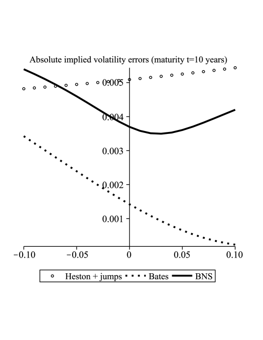
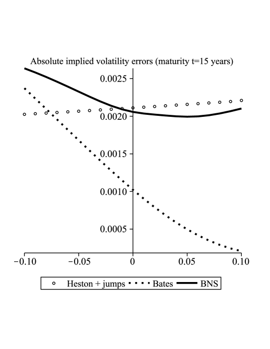
In this section we plot the difference $|\sigma_{\infty}(x)-\sigma_{t}(x)|$ for $t\in\{10,15\}$ and $x\in[-0.1,0.1]$ for the models with jumps from Section 6.1 (see Figure 1). In the case $t$ equals 10 years the error is approximately $45$ basis points (bp) with the strike $K$ ranging from $30\%$ to $200\%$ of the spot. At the maturity of 15 years the error is approximately $20$ bp and $K$ ranges between $20\%$ and $400\%$ of the spot.

In the cases of Heston with state-independent jumps and Bates with state-dependent jumps we took the following diffusion parameters

\lambda=1.15,\quad\zeta=0.2,\quad\theta=0.04,\quad\rho=-0.4

and the Lévy measure $\nu\left(\mathrm{d}\xi_{1}\right)=\alpha\mathrm{e}^{\alpha\xi_{1}}I_{\left\{\xi_{1}<0\right\}}\mathrm{d}\xi_{1}$ with $\alpha=0.6$ . The compensated cumulant generating function $\widetilde{\kappa}(u)$ (see (14) for the definition of $\widetilde{\kappa}(u)$ in Section 2.2.2 and note that it takes the same form in Section 2.2.3) is in this case given by

\widetilde{\kappa}(u)=\frac{u\left(u-1\right)}{\left(u+\alpha\right)\left(\alpha+1\right)}\qquad\text{for all }u\in\left(-\alpha,\infty\right).

In the case of the BNS model we took a pure-jump subordinator $J$ with Lévy measure $\nu\left(\mathrm{d}\xi_{2}\right)=ab\mathrm{e}^{-b\xi_{2}}I_{\left\{\xi_{2}>0\right\}}\mathrm{d}\xi_{2}$ . The cumulant generating function (16) is given by $\kappa(u)=au/(b-u)$ for $u<b$ . We used the following values for the parameters

a=1.4338,\quad b=11.6641,\quad\lambda=0.5783,\quad\rho=-1.2606,

which were taken from [Sch03, Section 7.3] where the model was calibrated to the options on the S&P 500.

Refer to caption — Figure 1. This figure contains the plots of the function $x\mapsto|\sigma_{\infty}(x)-\sigma_{t}(x)|$ in the interval $x\in[-0.1,0.1]$ for the models with jumps from Section 6.1 and maturities $t\in\{10,15\}$ . The values of the model parameters used are given in Section 6.2.

References

[Bat00] D.S. Bates. Post-’87 crash fears in the S&P 500 futures option market. Journal of Econometrics, 94:181–238, 2000.
[BNS01] O.E. Barndorff-Nielsen and N. Shephard. Non-Gaussian Ornstein–Uhlenbeck based models and some of their uses in financial economics. Journal of the Royal Statistical Society B, 63:167–241, 2001.
[DFS03] D. Duffie, D. Filipovic, and W. Schachermayer. Affine processes and applications in finance. Annals of Applied Probability, 13(3):984–1053, 2003.
[DL06] D.A. Dawson and Z. Li. Skew convolution semigroups and affine Markov processes. Annals of Probability, 34(3):1103–1142, 2006.
[DZ98] A. Dembo and O. Zeitouni. Large deviations techniques and applications. Springer, Berlin, 2 edition, 1998.
[FJ11] M. Forde and A. Jacquier. The large-maturity smile for the Heston model. Forthcoming in Finance & Stochastics, 2011.
[FJM10] M. Forde, A. Jacquier, and A. Mijatović. Asymptotic formulae for implied volatility in the Heston model. Proceedings of the Royal Society A, 466(2124):3593–3620, 2010.
[FJM11] M. Forde, A. Jacquier, and A. Mijatović. A note on essential smoothness in the Heston model. Forthcoming in Finance & Stochastics, 2011.
[GL11] K. Gao and R. Lee. Asymptotics of implied volatility to arbitrary order. Preprint available at http://ssrn.com/abstract=1768383, 2011.
[Hes93] S.L. Heston. A closed-form solution for options with stochastic volatility with applications to bond and currency options. Review of Financial Studies, 6(2):327–343, 1993.
[KR11] M. Keller-Ressel. Moment explosions and long-term behavior of affine stochastic volatility models. Mathematical Finance, 1(21):73–98, 2011.
[Lew00] A. Lewis. Option valuation under stochastic volatility. Finance Press, 2000.
[Roc70] A. T. Rockafellar. Convex Analysis. Princeton University Press, New Jersey, 1970.
[Sat99] K.I. Sato. Lévy Processes and Infinitely Divisible Distributions. Cambridge University Press, 1999.
[Sch03] W. Schoutens. Lévy Processes in Finance: Pricing Financial Derivatives. Wiley, 2003.
[Teh09] M.R. Tehranchi. Asymptotics of implied volatility far from maturity. Journal of Applied Probability, 46(3):629–650, 2009.

Large deviations and stochastic volatility with jumps: asymptotic implied volatility for affine models

Abstract.

Key words and phrases:

2000 Mathematics Subject Classification:

1. Introduction

2. Affine stochastic volatility models with jumps

Remarks.

Definition 1.

Remarks.

Definition 2.

Remark.

Proposition 3.

Proof.

2.1. SDE representation of affine stochastic volatility processes

Remarks.

2.2. Examples of affine stochastic volatility models

2.2.1. Heston model

2.2.2. Heston model with state-independent jumps

2.2.3. A model of Bates with state-dependent jumps

2.2.4. The Barndorff-Nielsen-Shephard (BNS) model

3. Large deviation principle and the Gärtner-Ellis theorem

Definition 4.

Definition 5.

Remarks.

Theorem 6.

4. Limiting cumulant generating function in affine stochastic volatility models

4.1. Non-degenerate affine stochastic volatility processes

Lemma 7.

Remarks.

Theorem 8.

Remark.

Lemma 9.

Proof.

Remark.

Theorem 10.

Corollary 11.

4.2. Degenerate affine stochastic volatility models

Proposition 12.

5. Rate functions and the option prices far from maturity

Remarks.

Theorem 13.

Remarks.

Proof.

6. Asymptotic behaviour of the implied volatility

Remarks.

Theorem 14.

Remark.

Proof.

Corollary 15.

Proof.

Remarks.

6.1. Examples of limiting smiles

6.1.1. Heston model

6.1.2. Heston model with state-independent jumps

6.1.3. A model of Bates with state-dependent jumps

6.1.4. The Barndorff-Nielsen-Shephard model

6.2. How close are the formula σ∞​(x)\sigma_{\infty}(x) and the implied volatility σt​(x)\sigma_{t}(x) for large maturity?

References

Large deviations and stochastic volatility with jumps:
asymptotic implied volatility for affine models

6.2. How close are the formula $\sigma_{\infty}(x)$ and the implied volatility $\sigma_{t}(x)$ for large maturity?