Large sample scaling analysis of the Zig-Zag algorithm for Bayesian inference
Abstract
Piecewise deterministic Markov processes provide scalable methods for sampling from the posterior distributions in big data settings by admitting principled sub-sampling strategies that do not bias the output. An important example is the Zig-Zag process of [Ann. Stats. 47 (2019) 1288 - 1320] where clever sub-sampling has been shown to produce an essentially independent sample at a cost that does not scale with the size of the data. However, sub-sampling also leads to slower convergence and poor mixing of the process, a behaviour which questions the promised scalability of the algorithm. We provide a large sample scaling analysis of the Zig-Zag process and its sub-sampling versions in settings of parametric Bayesian inference. In the transient phase of the algorithm, we show that the Zig-Zag trajectories are well approximated by the solution to a system of ODEs. These ODEs possess a drift in the direction of decreasing KL-divergence between the assumed model and the true distribution and are explicitly characterized in the paper. In the stationary phase, we give weak convergence results for different versions of the Zig-Zag process. Based on our results, we estimate that for large data sets of size , using suitable control variates with sub-sampling in Zig-Zag, the algorithm costs to obtain an essentially independent sample; a computational speed-up of over the canonical version of Zig-Zag and other traditional MCMC methods.
Keywords and phrases: MCMC, piecewise deterministic Markov processes, fluid limits, sub-sampling, multi-scale dynamics, averaging.
1 Introduction
Piecewise deterministic Markov processes [PDMPs, 21] are a class of non-reversible Markov processes which have recently emerged as alternatives to traditional MCMC methods based on the Metropolis-Hastings algorithm. Practically implementable PDMP algorithms such as the Zig-Zag sampler [11], the Bouncy Particle Sampler [16] and others [18, 31, 33, 12, 7, 8, 29] have provided highly encouraging results for Bayesian inference as well as in Physics [26, for example]. As a result, there has been a surge of interest in the Monte Carlo community to better understand the theoretical properties of PDMPs [see e.g. 24, 22, 1, 9, 15, 14, 13]. This body of work demonstrates powerful convergence properties with impressive scalability as a function of the dimension.
However, the most exciting property of PDMPs, at least for statistical applications is that of principled sub-sampling [11], whereby randomly chosen subsets of data can be used to estimate likelihood values within the algorithm without biasing its invariant distribution. The authors only cover sub-sampling for the Zig-Zag algorithm, although the unbiasedness property holds for a rather general class of PDMP MCMC algorithms. This unbiasing property is in sharp contrast to most MCMC methods [32, 28, 5], although see [19]. In fact, [11] gives experiments to show that even for data sets of large size , subsets of size can be used to estimate the likelihood, producing a computational speed-up of . This leads to the property of superefficiency whereby, after initialization, the entire running cost of the algorithm is dominated for large by the cost of evaluating the likelihood once. In [11], the authors provide two algorithms which utilise this sub-sampling idea: the straightforward ZZ-SS algorithm together with a control-variate variant ZZ-CV which will be formally introduced in Section 2.
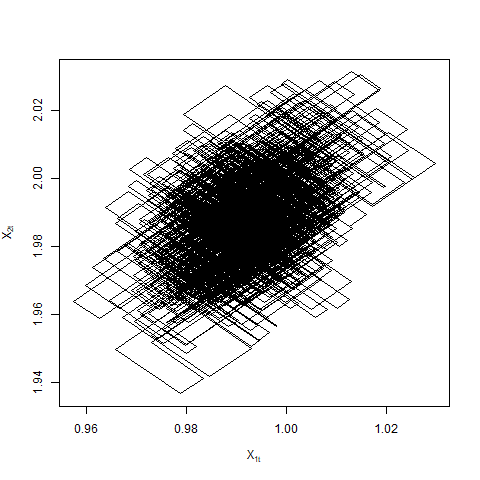
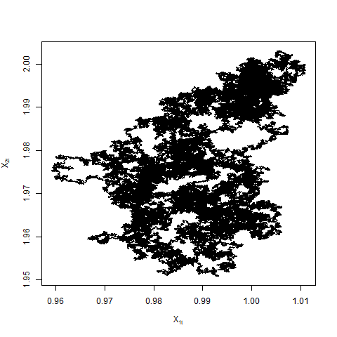
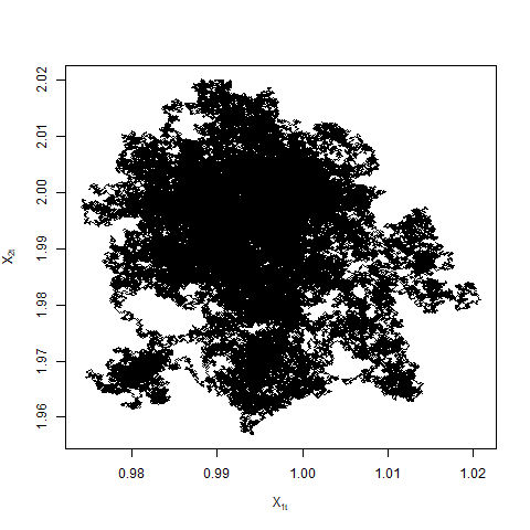
In [11], the authors also point out that although principled sub-sampling gives these dramatic improvements in implementation time, the dynamics of ZZ-SS and ZZ-CV differ from that of canonical Zig-Zag: sample paths exhibit more diffusive behaviour to the extra velocity switches induced by the variation in the estimate of the likelihood. This might lead to slower convergence and inferior mixing of the underlying stochastic process (see Figure 2). For one-dimensional Zig-Zag, [9] studies the diffusive behaviour resulting from excess switches outside of a statistical context. In [2], the authors show that canonical Zig-Zag has superior mixing (in the sense of minimising asymptotic variance for estimating a typical function) than any alternative with excess switches. Since both ZZ-SS and ZZ-CV can be viewed as Zig-Zag algorithms with excess switches, this raises the question of whether the inferior mixing of sub-sampling Zig-Zag algorithms relative to their canonical parent might negate their computational advantage.
To date, no work has been done to study the extent of the algorithm mixing deterioration caused by these excess switches induced by sub-sampling. The goal of this work is to give the first rigorous theoretical results to understand this problem. We shall study the behaviour of the various Zig-Zag algorithms for large data sets, interplaying closely with large-sample Bayesian asymptotics, both in the correctly specified and misclassified cases.
Our contributions in this paper are as follows.
-
1.
For the Zig-Zag algorithm, we study the effect of sub-sampling on the dynamics of the underlying stochastic process as the data set size increases to infinity. In Theorem 3.3, we give weak convergence results for the trajectories of the process to smooth solutions of a system of ODEs. These ODEs can be explicitly characterized as presented in equation (3.4).
-
2.
We also study the effect of sub-sampling on the algorithm mixing in the stationary phase. We find that as becomes infinitely large, the trajectories of ZZ-SS converge to a reversible Ornstein-Uhlenbeck process as given in Theorem 4.2, mixing in time. Whereas, both canonical Zig-Zag and ZZ-CV converge to a PDMP that mixes in time as presented in Theorem 4.6 and 4.11.
-
3.
Our theoretical study leads to further guidance for implementing sub-sampling with Zig-Zag. In particular, our results highlight that for heavy-tailed models the vanilla sub-sampling outperforms ZZ-CV in the tails. In Section 5, we propose a mixed sub-sampling scheme which in addition to being exact, supersedes both ZZ-SS and ZZ-CV in performance.
-
4.
Finally, we outline how these methods can be generalised to more general classes of PDMPs.
In parametric Bayesian inference, given sufficient regularity in the model and the true data-generating distribution, it is well known that the posterior distribution converges to a degenerate distribution as the data set size irrespective of whether the true data-generating distribution belongs to the assumed model or not [6, 25]. The point of concentration is the parameter value (if it exists and is unique) minimizing the Kullback-Liebler (KL) divergence between the true data-generating distribution and the assumed model. In well-specified settings, this is the same as the true parameter. Our results in the transient phase (Section 3) show that for large , the Zig-Zag trajectories behave like deterministic smooth flows with a drift pushing them in the direction of decreasing KL-divergence. While the canonical Zig-Zag attains optimal speed () in the limit, the sub-sampling versions remain sub-optimal with a damping factor that depends on the model. In particular, we find that the vanilla sub-sampling starts with the optimal speed at infinity, suffering from an extreme slowdown as the process gets closer to the minimizer. On the other hand for sub-sampling with control variates, the drift remains positive at stationarity achieving optimal speed for model densities that are log-concave in the parameter.
Let be the unique parameter value minimizing the KL-divergence between the true data-generating distribution and the true parameter. In stationarity, the high concentration of the posterior mass around restricts the movement of the Zig-Zag process. Indeed, the canonical Zig-Zag remains close to once it hits (Theorem 4.1). In general, the smooth approximations from the transient phase are no longer informative since they only capture the large-scale movements of the Zig-Zag trajectories. Let be a sequence of suitable estimators of such that the Bernstein von-Mises Theorem holds: in the rescaled coordinate , the posterior converges to a Gaussian distribution with zero mean and variance-covariance matrix given by the inverse of the Fisher’s information [25]. Under regularity conditions, can be taken to be the maximum likelihood estimators (MLE) for the (possibly misspecified) model. In the coordinate thus, the trajectories of the Zig-Zag process have a non-trivial limit. Although, the canonical Zig-Zag and control variate Zig-Zag mix at a rate in contrast to for the vanilla sub-sampling (Section 4).
In stationarity, the computational complexity of a sampling algorithm can be described as:
| computational complexity | |||
For Zig-Zag algorithms this further breaks down to
| computational complexity | |||
The canonical Zig-Zag incurs an cost per proposed switch because the full data set needs to be processed to compute the switching rate at each proposed switching time. In contrast to this, the sub-sampling versions only cost per proposed switch as only a small subset of the whole data set is utilized to estimate the switching rate at each proposed switching time. The time taken to obtain an essentially independent sample is for canonical Zig-Zag and Zig-Zag with control variates whereas it is for vanilla sub-sampling. The number of proposed switches depends on the computational bounds on the switching rates used in the implementation of the algorithm. In the rescaled coordinate, the effective switching rates are of the magnitude for canonical Zig-Zag and Zig-Zag with control variates and for vanilla sub-sampling. Assuming the computational bounds are tight and an efficient implementation of the algorithm is possible, Table 1 summarizes the computational complexity of different versions of the Zig-Zag algorithm in the stationary phase.
| Algorithm | time to an essentially ind. sample | proposed switches per unit time | cost per proposed switch | computational complexity |
| ZZ | ||||
| ZZ-SS | ||||
| ZZ-CV |
The computational complexity of the canonical Zig-Zag and Zig-Zag with vanilla sub-sampling per independent sample is provided tight computational bounds are available. In contrast, Zig-Zag with control variates achieves a computational speed-up of when the sequence of reference points is chosen sufficiently close to the sequence of estimators .
The paper is constructed as follows. Section 2 details the Zig-Zag algorithm applied to the Bayesian setting with i.i.d observations along with a discussion of the sub-sampling method. Section 3 contains our main results on the transient phase of the algorithm. We study the stationary phase separately in Section 4. In Section 5, we discuss the results of the transient phase in more detail along with some illustrations on simple models. We conclude with a final discussion in Section 6. All the proofs can be found in the Appendix.
2 Zig-Zag process for parametric Bayesian inference with i.i.d. observations
In this section, we review how the Zig-Zag process can be designed to sample from a Bayesian posterior distribution in the setting where the data are assumed to be generated independently from a fixed probability model. For details, we refer to [11].
2.1 Designing Zig-Zag process for Bayesian inference
The dimensional Zig-Zag process is a continuous time Markov process that evolves on the augmented space where . We refer to and as position and velocity process respectively. The Zig-Zag process is completely characterized by a collection of continuous switching rates where for all . Given , has right-continuous paths in such that,
and the -th coordinate of jumps between and according to an inhomogeneous Poisson process of intensity independently of other coordinates.
Given independent and identically distributed data points , consider the classical Bayesian posterior density, , given by
for some probability density function and prior density . Define the potential function by,
| (2.1) |
For , define the flip operator , which flips the -th component of : for , and for . Suppose the switching rates are linked to via
| (2.2) |
Then, the Zig-Zag process with switching rates given by (2.3) has an invariant distribution whose marginal distribution on is equivalent to [11]. A necessary and sufficient condition for (2.2) to hold is that there exists a continuous such that for all , and
| (2.3) |
The switching rates for which in (2.3) are called canonical switching rates and the corresponding Zig-Zag process the canonical Zig-Zag process. We will denote the canonical rates by . The function itself is called the excess switching rate.
2.2 Sub-sampling with Zig-Zag
The implementation of Zig-Zag is usually carried out by Poisson thinning. This involves proposing to switch the velocity according to a Poisson process with a bounding jump intensity and then accepting or rejecting the proposed switch with a certain probability. Each accept-reject step requires evaluation of one of the s. Observe that admits the following additive decomposition,
| (2.4) |
If it costs to compute each gradient term in the summation, the canonical rates, , incur an computational cost per evaluation.
Fix and let be random (given data) such that it unbiasedly estimates the sum in (2.4) i.e. . Provided that the cost of generating one realization of is , the sub-sampling idea is to replace, at the accept-reject step, the sum (2.4) by a random realization of . The effective switching rate of this procedure is then given by, [11]. Observe that the new switching rate preserves the invariance of the target distribution i.e.
which is equivalent to (2.3). Jensen’s inequality implies that
Hence, any sub-sampling procedure results in a possibly larger effective switching rate. However, the computational cost per proposed switch for this procedure is bounded above by the cost of generating one random realization of .
We will consider unbiased estimators for (2.4) based on random batches of size from the whole data set. In our asymptotic study in later sections, may be chosen to depend explicitly on , e.g., , or be held fixed, i.e. . For now, we will suppress the dependence on . Let be functions from to such that for all ,
| (2.5) |
For , let be a simple random sample (without replacement) of size from . Then, is an unbiased estimator of . The effective switching rates are given by,
| (2.6) |
where denotes the collection of all possible simple random samples (without replacement) of size from . Given (2.5), it is easy to observe that as defined in (2.6) satisfy (2.3) for all and . Hence, the resulting process is still exact. In this paper, we analyze the following two choices of suggested in [11]. Our results, however, can be easily extended to other choices.
Zig-Zag with sub-sampling (ZZ-SS): The vanilla sub-sampling strategy where we set
| (2.7) |
This choice of is suitable when the gradient terms in (2.4) are globally bounded i.e. there exist positive constants such that for all and . We denote the switching rates by and call this process Zig-Zag with sub-sampling (ZZ-SS).
Zig-Zag with Control Variates (ZZ-CV): The second choice is suitable when the gradient terms are globally Lipschitz. The Lipschitz condition allows the use of control variates to reduce variance in the vanilla sub-sampling estimator of .
Let be a reference point in the space. The control variate idea is to set
| (2.8) |
For a suitably chosen reference point, writing as above helps reduce its variability as is varied [11]. Note that the reference point is allowed to depend on the data . In practice, a common choice would be to use the MLE or the posterior mode, however, this might not always be the best choice as we will show in the later sections. Finally, we suppose throughout this paper that is chosen and fixed before the Zig-Zag algorithm is initialized. Our results in the later sections, although, advocate for continuous updation of the reference point. We denote the switching rates by and call the corresponding process Zig-Zag with control variates (ZZ-CV).
Finally, note that when , the rates in (2.6) reduce to canonical rate irrespective of the choice of . We will drop the subscript “ss”, “can”, and “cv” from when the choice is understood from the context or when we are talking about switching rates in general.
2.3 Technical setup
Let be an arbitrary complete probability space, rich enough to accommodate all the random elements defined in the following. This probability space will be used as the primary source of randomness and the data sequence will be defined on it via a data-generating process (see below). The Zig-Zag process will be viewed as a random element on conditioned on the data. All our limit theorems will be of type “weak convergence (in Skorohod topology) in probability” or “weak convergence (in Skorohod topology) almost surely”.
Denote the observation space by and the space of probability measures on by . Let be a data-generating process such that for some i.e. is the push-forward of by . Fix a model for . Suppose that and are absolutely continuous with respect to a common base measure on . Let be the continuous density of with respect to and for each , let be the respective density of .
Let be a sequence of random elements defined on . Let denote the dataset size. For all , let be the random measure on such that,
For any fixed , given , is the classical Bayesian posterior for under a uniform prior. Since we will be concerned with asymptotic behaviour for large we can work under the assumption of a uniform prior without loss of generality.
For each , let be a statistic. Define the sequence of reference points
| (2.9) |
to be a random element on taking values in . We will assume that the sequence is chosen and fixed as soon as a model is identified.
2.4 Notation and assumptions
We will use to denote the Euclidean norm in and to denote the induced matrix norm. For any , denotes the positive part of i.e. . If is differentiable, we denote the gradient vector by . If is twice differentiable, we use to denote the Hessian of . For , absolutely continuous in its first argument, we will use to denote the partial derivative of with respect to . We denote the dimensional vector of all s by and the identity matrix by .
Define, when it exists, and . We will use to denote the corresponding random element when . Given , we will use and to denote and respectively. We make the following assumptions on the model and observed data.
Assumption 2.1 (Smoothness).
For each , . There exists such that for all ,
Assumption 2.2 (Moments).
For all , the following moment condition is satisfied:
Assumption 2.3 (Unique minimizer of the KL-divergence).
The KL-divergence of the assumed model relative to the true data-generating distribution is finite and uniquely minimized at , i.e.:
Assumption 2.4 (Bernstein von-Mises Theorem).
There exists a sequence of estimators satisfying for all such that,
-
(i)
in probability as .
-
(ii)
Define . Then,
in probability as .
-
(iii)
Let denote the collection of Borel sets on . Then,
as in probability. Here, denotes the (multivariate) Gaussian distribution with mean vector and variance-covariance matrix .
Assumptions 2.1 and 2.2 are used throughout the paper and provide sufficient regularity in the model and on the data. Although, they can be relaxed to a certain degree (see Remark 3.5), we do not pursue that generalization in this paper. Assumptions 2.3 and 2.4 are used in the stationary phase to ensure the posterior converges at a certain rate to a point mass as goes to infinity. Part (ii) of Assumption 2.4 further implies asymptotic normality of the posterior to allow for non-trivial limits in the stationary phase. Under regularity conditions, the sequence of MLE i.e. satisfies the conditions in Assumption 2.4[25]. For our main results in Sections 3 and 4, we do not assume that , i.e. the model is well-specified. If indeed it does, in Assumption 2.3 is such that .
3 Fluid limits in the transient phase
This section establishes fluid limits for the Zig-Zag process in Bayesian inference. We consider the identifiable situation where, as more data becomes available, the posterior distribution contracts to a point mass. In this case, the gradient of the log-likelihood grows linearly in and, as a result, the switching intensities become proportionally large (see Proposition 3.1). This results in a limiting process that switches immediately to a ‘favourable’ direction and asymptotically the Zig-Zag process behaves as the solution of an ordinary differential equation as we will detail below. Throughout this section, we assume the following about the sequence of reference points defined in (2.9).
Assumption 3.1.
There exists an defined on such that , is independent of , and for the sequence of reference points we have that , almost surely.
For each , let be a Zig-Zag process targeting with switching rates defined as in (2.6). For each and , define the sets
| (3.1) |
Let . Since the switching rates are continuous, is open. Define for each ,
where we set if . For some cemetary state , we consider the sequence of stopped processes defined as,
The stopped process is again a PDMP that is sent to the cemetery state as soon as the position process enters and stays there. The corresponding semigroup can be appropriately modified [20]. However, we introduce the cemetery state only for the sake of rigour; it can be ignored for all practical purposes.
The following proposition is a consequence of the strong law of large numbers for statistics and applies to any choice of switching rates as defined in Section 1. We remind the reader that we omit the subscripts “can”, “ss”, and “cv” here.
Proposition 3.1.
The proof is located in the Appendix A. Proposition 3.1 indicates that the switching rates are . This means that on average the process flips direction every time. But since the position component has unit speed in each coordinate, the process only travels distance between each direction flip. As goes to infinity, the number of switches per unit time goes to infinity but the distance travelled between each switch becomes infinitesimally small. Consequently, on the usual time scale, the position component appears to traverse a smooth path and is feasibly approximated by the solution to an ODE.
For each , define the sequence of drifts such that,
| (3.2) |
for all . Then, is well-defined. For each fixed , let be as in the Proposition 3.1. Define, for each ,
and let . Note that the sets may vary with e.g. in ZZ-CV where the sum of switching rates depends on the limiting reference point. For each , define the asymptotic drift as,
The following proposition follows easily from the last one.
Proposition 3.2.
The proof is located in the Appendix A. Extend the solution to as,
We now state the main result of this section.
Theorem 3.3.
The proof is located in the Appendix B.
Remark 3.4.
Theorem 3.3 establishes smooth approximation for the Zig-Zag trajectories until they enter . This is not a limitation in approximation due to the Markov property; the fluid limits apply as soon as the process leaves .
Remark 3.5.
The deterministic approximation in Theorem 3.3 is a consequence of multi-scale dynamics in the components of the Zig-Zag process and is not special to the Bayesian settings. In general, suppose switching rates and the position process moves at a speed . Similar fluid limits can be obtained whenever .
The asymptotic drift has the following form (see Appendix A):
| (3.4) |
where is the asymptotic switching rate from Proposition 3.1 and . In the large limit, the function entirely characterizes the dynamics of the Zig-Zag trajectories. To understand the effect of different sub-sampling schemes, it is sufficient to understand how the denominator behaves in each situation. For the canonical Zig-Zag,
| (3.5) |
for all such that the expectation is non-zero. This corresponds to the optimal speed achievable by the Zig-Zag process i.e. . Now suppose the subsample size is fixed. Then,
| (3.6) |
where . Similarly, for Zig-Zag with control variates the denominator is given, when the expectation is non-zero, by
| (3.7) |
where and is as in Assumption 3.1.
Remark 3.6.
Note that, as a consequence of the above, the asymptotic drift for ZZ-CV is random in terms of . However, the procedure for choosing reference points is fixed before implementing the algorithm. Hence, the value of is known as soon as the data is observed.
Remark 3.7.
For any , it follows from Jensen’s inequality that for all and irrespective of the sampling scheme. When as , we show in the Appendix A that for both ZZ-SS and ZZ-CV. Thus, larger subsamples lead to faster convergence. However, it can be shown that a subsample of size does not produce a two times increase in the drift. However, a subsample of size incurs twice the computational cost at each proposed switching time. Thus it seems optimal to select a subsample of size .
Remark 3.8.
The expression for differs for different sequences of switching rates but by the definition of , the denominator in (3.4) is always positive. And so the limiting flow drifts in the direction of decreasing i.e. decreasing KL-divergence between and the model . When Assumption 2.3 is satisfied, this would imply that the limiting flow drifts towards . This is expected behaviour as the posterior mass concentrates around as goes to infinity and the Zig-Zag process tries to find its way towards stationarity. The denominator in (3.4) is the damping factor that quantifies the loss in speed due to sub-sampling. For canonical Zig-Zag, (3.5) implies that the corresponding ODE has the optimal drift i.e. or depending on the relative location of . For ZZ-SS and ZZ-CV in general, . Although in some cases, ZZ-CV achieves optimal speed as illustrated in Section 5.
The sets take different forms for different switching rates. For canonical Zig-Zag, each is the hypersurface . For ZZ-SS, each since the sum is always positive. For ZZ-CV with reference point , the sets can be either as small as the empty sets in the ZZ-SS case e.g. if the reference point is not close to any of the conditional modes. Or they can be as large as the hypersurfaces in the canonical case e.g. when the model density is Gaussian in which case the ZZ-CV switching rates are equivalent to the canonical Zig-Zag irrespective of the reference point . However, note that since the canonical rates are the smallest, for any of the form (2.6),
for all . And so, for any choice of the switching rates,
![[Uncaptioned image]](https://cdn.awesomepapers.org/papers/99f9c758-9a14-4943-8968-9acfdfbcb168/zzlr_ss_1_transient.png)
![[Uncaptioned image]](https://cdn.awesomepapers.org/papers/99f9c758-9a14-4943-8968-9acfdfbcb168/zzlr_diffusive_behaviour.png)
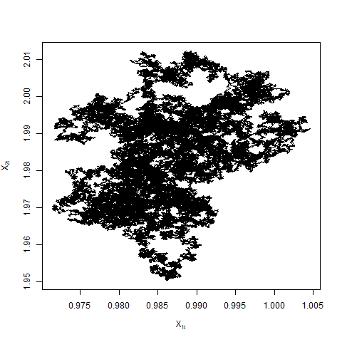
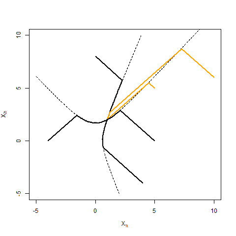
When hits for some , the total switching rate, and hence the momentum, in the th coordinate, becomes zero. However, other coordinates may still carry momentum and affect the overall dynamics of the process. This leads to interesting behaviour: the process either jumps back out of with a certain velocity or remains stuck to for a random amount of time (see Figure 3). It is not straightforward to extend the proof of Theorem 3.3 as the process behaves dimensional on these sets. Consequently, the stability analysis of the sets is beyond the scope of this paper.
4 The stationary phase
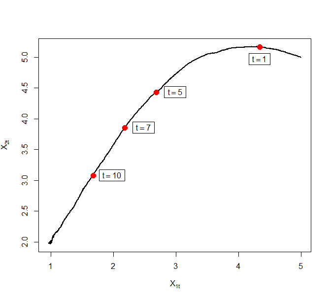
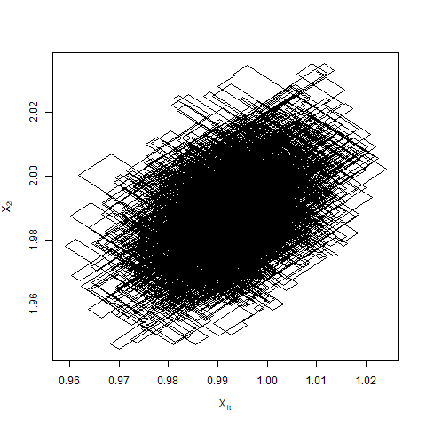
As noted in Section 1, the fluid limits only capture deviations in the Zig-Zag trajectories that are big enough on the usual space scale. Suppose Assumptions 2.3 and 2.4 hold. As becomes large the posterior concentrates around . Consequently, the posterior mass inside the interval goes to for any . This restricts the movement of the Zig-Zag process to regions close to (see Figure 4). Once the Zig-Zag process targeting hits , it is hence reasonable to expect that the process stays within distance of with high probability. The following result illustrates this in one dimension under the additional assumption of unimodality of the posterior. The proof is located in the Appendix C.
Theorem 4.1.
A sufficient condition for the assumption in Theorem 4.1 to hold is when is log-concave as a function of for any (where is the data generating density for a given parameter ), and satisfying exists. Since the sequence converges to in probability, Theorem 4.1 implies that once it gets close to , the canonical Zig-Zag stays close to as . To obtain a non-trivial limit in stationarity the process needs to be analyzed on its natural scale which depends on the rate of the posterior contraction. Consider the reparameterization,
The posterior distribution in terms of the parameter converges to a multivariate Gaussian distribution. Under this reparameterization, it is natural to expect that the Zig-Zag process converges to a non-trivial stochastic process targeting the asymptotic Gaussian distribution.
In the coordinate, the Zig-Zag process has a speed . However, the switching rates for ZZ-SS and ZZ-CV in terms of may differ in magnitudes and hence require separate analysis. In what follows we assume that the process starts from stationarity i.e. for all .
4.1 Zig-Zag with sub-sampling (without control-variates)
We first consider ZZ-SS. The -th switching rate in the rescaled parameter is written as,
| (4.1) |
For large , the above quantity is . In coordinate, the velocity component still oscillates at rate while the position component moves with speed . This is, once again, a situation of multi-scale dynamics as in the last section. It is tempting to scale down the time by a factor and do the averaging as in Theorem 3.3. But consider,
Thus, the difference in the rates in opposite directions is while the sum remains . As a result, the drift goes to and the averaging leads to a trivial fluid limit (see Appendix C). However, in the parameter, the above observations imply that the infinitesimal drift and the infinitesimal variance in the position component is . This suggests that the process is moving on a diffusive scale.
Let be fixed for some . For each , let be a ZZ-SS process targeting the posterior with fixed sub-sample size . For each , define by
| (4.2) |
We have the following result.
Theorem 4.2.
The proof is located in the Appendix C.
Remark 4.3.
The limiting diffusion is invariant with respect to the limiting Gaussian distribution in the Bernstein von-Mises theorem. The matrix in 4.3 is the damping factor quantifying the loss in mixing due to sub-sampling.
Remark 4.4.
When the model is well-specified i.e , . By Jensen’s inequality,
Thus, using a batch size of is not times better than using a batch size of . In terms of the total computational cost, it is thus optimal to choose .
Remark 4.5.
Since we do not rescale time, Theorem 4.2 implies that the ZZ-SS process requires time to obtain an (approximately) independent sample. Assuming computational bounds are of the same order as the switching rate i.e. , the total computational complexity of the ZZ-SS sampler is thus estimated to be .
4.2 Zig-Zag with Control Variates
Next, we consider the ZZ-CV process in the coordinate. Let be a random sequence of reference points in as used in ZZ-CV. Define for all i.e. . For any observed value of , the -th switching rate in parameter is given by
| (4.4) |
where
The magnitude of the switching rates depends explicitly on the sequence of reference points and their distance to . A reasonable choice for is to ensure is sufficiently close to . Motivated by the scaling arguments in [11], we suppose that the reference points are chosen such that i.e. converges to some finite random element. Then, it can be shown that the ZZ-CV switching rates in coordinate are of magnitude . This implies, in the coordinate, the position and the velocity process mix at the same rate which is . Slowing down time by a factor brings both the components back to the unit time scale. Consequently, the limiting process is a Zig-Zag process with an appropriate switching rate.
Let be fixed for some . For each , let be a ZZ-CV process targeting the posterior with reference point and fixed sub-sample size . Define
We have the following result.
Theorem 4.6.
Suppose Assumptions 2.1 - 2.4. Let be such that in -probability. Moreover, is independent of and . Then converges weakly (in Skorohod topology) in probability to where is a (random) -dimensional stationary Zig-Zag process with, conditional on , -th switching rate
| (4.5) | ||||
where is the -th column of the Hessian matrix and are independent of .
The proof is located in the Appendix C.
Remark 4.7.
Observe that for any value of ,
The limiting Zig-Zag process is invariant with respect to the limiting Gaussian distribution with mean vector and covariance matrix given by the inverse of .
Remark 4.8.
As in the case of fluid limits, the limiting process is a random Zig-Zag process depending on the statistic used to generate reference points. When is such that for , then almost surely. The limiting switching rate reduces to,
Remark 4.9.
In general, the limiting Zig-Zag process is not canonical. By Jensen’s inequality, for any fixed ,
However, for the exponential family of distributions represented in their natural parameters, the Hessian is independent of . The limiting rate then becomes equivalent to the canonical rate. In general, the amount of excess quantifies the loss in efficiency due to sub-sampling.
Remark 4.10.
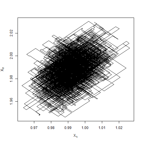
The difference in the switching rates in opposite directions for ZZ-CV is the same as ZZ-SS i.e. . The limiting dynamics are then governed only by the magnitude of the sum of the switching rates. The assumption that in Theorem 4.6 cannot be dropped. In general, suppose for some , then the switching rates or the sum of the switching rates are of the magnitude . In particular when , the sum of the rates is and the process is once again in the diffusive scale as in the case of ZZ-SS. We do not pursue this any further in this paper but see Figure 5 for examples of Zig-Zag trajectories when .
Suppose now the sub-sample size varies with . The canonical Zig-Zag corresponds to the case . If is large when is large, it is reasonable to expect that ZZ-CV behaves similarly to the canonical Zig-Zag. Although it can be argued, as in the case of ZZ-SS, that is optimal in terms of the total computational cost of the algorithm. The following result is for completeness. It shows that if as , the limiting process does not depend on the reference points in ZZ-CV and is equivalent to the canonical Zig-Zag. Once again, the limiting process is invariant with respect to the limiting Gaussian distribution.
Theorem 4.11.
In Theorem 4.6, suppose that the sub-sample size such that for all , and as . Then the limiting process is a stationary Zig-Zag process with switching rates
where and is the -th column of .
The proof is located in the Appendix C.
Remark 4.12.
Theorem 4.11 and 4.6 verify the observations presented in [11] that, starting from equilibrium, the canonical Zig-Zag and the ZZ-CV process require a time interval of to obtain an essentially independent sample. Provided the computational bound used in the sampler is , this can be achieved in proposed switches. However, at each proposed switch, canonical Zig-Zag incurs computational cost while for fixed subsample sizes, ZZ-CV costs only , resulting in significant benefits.
5 Illustration of fluid limits
In this section, we go back to the transient phase and consider the fluid limit in more detail. Recall the expression for asymptotic drift (3.4) that is,
where . Let , and denote the asymptotic drifts for canonical Zig-Zag, ZZ-SS and ZZ-CV respectively obtained by putting (3.5), (3.6), and (3.7) in (3.4). Note that since the data is almost surely non-degenerate, the drift for ZZ-SS is well-defined on the whole space i.e. almost surely. For canonical Zig-Zag, . For ZZ-CV on the other hand, the set depends on the model and the observed value of . For example’s sake, when the model is Gaussian.
5.1 Toy examples
We illustrate fluid limits in some simple examples. Suppose for some . Then, . We first look at some toy models in one dimension.
-
•
Gaussian model: Suppose and . Then and for ZZ-SS. But since is linear in both and , using control variates makes the variance in equal to . To wit,
Hence, the ZZ-CV becomes equivalent to the canonical Zig-Zag in this case. We get,
In general, for one-dimensional models with log-concave densities, it can be shown that ZZ-CV will always be equivalent to the canonical Zig-Zag.
-
•
Laplace model: Suppose and . The log-density is not continuously differentiable on a null set and hence, violates the smoothness assumption needed for fluid limits. However, defining to be the weak derivative with respect to of , we get,
Let . Then,
Given the form of function, note that for any , only depends on the direction of relative to . Then the denominator term in only depends on the location of and the direction of relative to . Let . Let be the observed value of . When , i.e. , the drift is given by,
On the other hand when , , and we have,
Hence, the fluid limit travels with optimal speed till after which it slows down until it reaches where it settles. Appropriate choice of control variates, however, can make the process more efficient. Suppose the sequence of reference points is chosen such that almost surely. Then, almost surely and the asymptotic drift is equivalent to the canonical drift,
In addition if , the ZZ-CV is equivalent to the canonical Zig-Zag for corresponding .
-
•
Cauchy model: Suppose and . Then, . The explicit expression is hard to calculate in this case. In particular, suppose almost surely and let . Then,
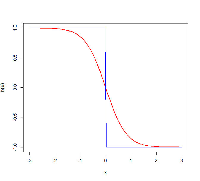
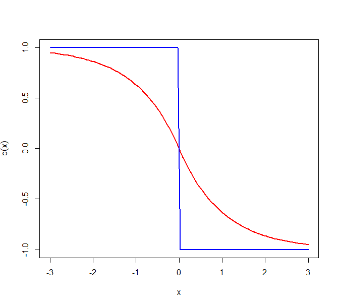
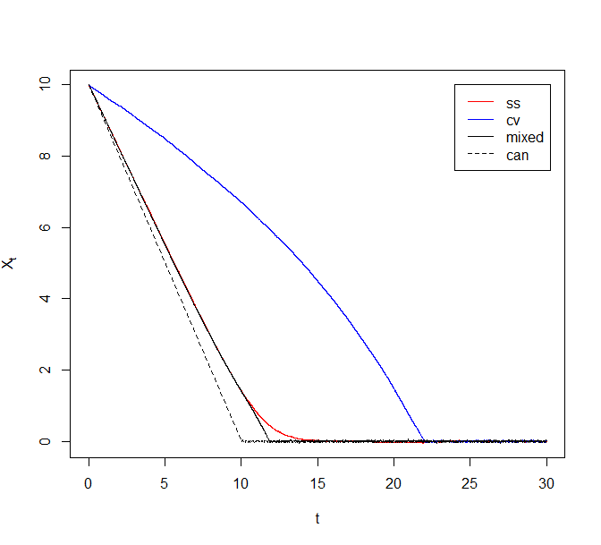
Figure 6 plots the asymptotic drifts for the above models for canonical Zig-Zag, ZZ-SS, and ZZ-CV (when almost surely). The subsample size and . As the calculations above show, when the model is Normal or Laplace, ZZ-CV is equivalent to canonical Zig-Zag. However, we see that for the Cauchy model, ZZ-CV is sup-optimal near . Indeed, . The more interesting feature of these plots is the Cauchy model where, contrary to expectations, ZZ-CV performs worse than ZZ-SS. Later in Section 5.3, we will see that this is a consequence of heavy tails and is generally true.
5.2 Bayesian logisitic regression
Consider a set of observations with and , . We assume a Bayesian logistic regression model on the observations such that given a parameter and covariate , the binary variable has distribution,
Additionally, since we are interested in large sample asymptotics, we suppose that the covariates , for some probability measure on with Lebesgue density . Under a flat prior assumption, the posterior density for the parameter is,
The corresponding potential function is given by,
and so,
Let denote the probability . In the case of a well-specified model with true model parameter it follows, after conditioning on , that
Moreover, we get
The -th coordinate of the asymptotic drift for ZZ-SS corresponding to sub-sample size is then
Similarly, for ZZ-CV, observe that for any given ,
In particular, when almost surely, the above simplifies and we get the asymptotic ZZ-CV drift,
Finally,
for all for which the denominator is non-zero.
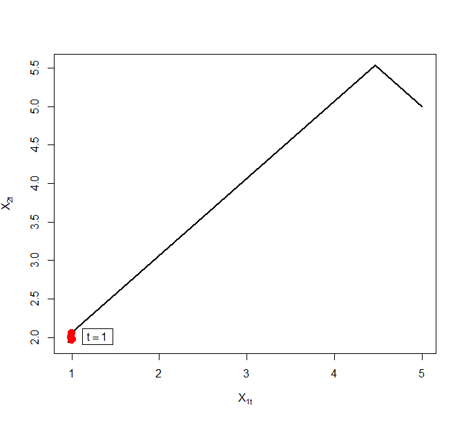
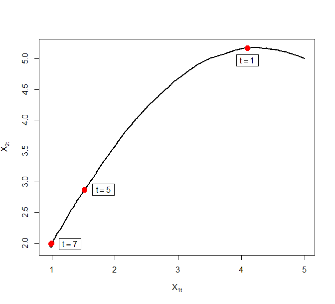
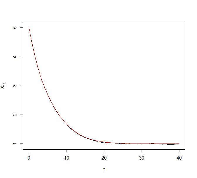
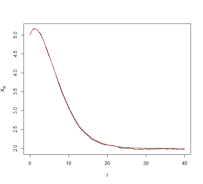
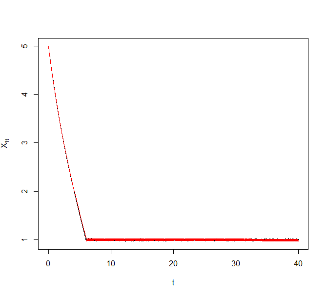
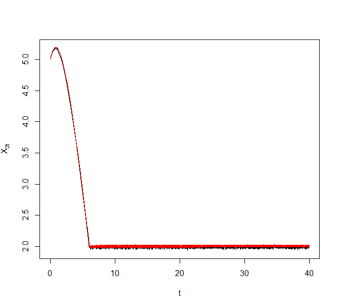
As an illustrative example, we generated a synthetic data set of size from the above model with and . Figure 8 plots trajectories of the Zig-Zag process under different sub-sampling schemes targeting the corresponding Bayesian posterior. The reference point for ZZ-CV was chosen to be a numerical estimate of the MLE. The black curve denotes the actual Zig-Zag process trajectories and the superimposing red curve denotes the solution to the asymptotic ODE.
5.3 Comparison of ZZ-SS and ZZ-CV
As noted before, comparing drifts for different sub-sampling schemes is equivalent to comparing the denominator in (3.4). Looking at the expressions for the denominator in (3.6) and (3.7), it is not obvious when one is faster than the other. Figure 6 already illustrates an example where, contrary to expectations, ZZ-CV performs worse than ZZ-SS.
Although the results so far do not assume well-specified models, in what follows, we suppose for some . Given the smoothness conditions, we have . For the ease of exposition, we set . The asymptotic drift reduces to
When the model is heavy-tailed in the sense that for all , , the dominated convergence theorem implies that the multiplicative factor in the above expression goes to as goes to infinity for each fixed value of .
Corollary 5.1.
For heavy tailed models, i.e. when for all , there exists an such that for all , , . Moreover, for all .
Hence, the ZZ-SS will outperform ZZ-CV in tails in terms of the speed of convergence when the model is heavy-tailed. This happens because control variates in general require correlation between terms to offer variance reduction. For heavy-tailed models, as the function becomes flatter in the tails, the terms and become increasingly uncorrelated. Consequently, the ZZ-CV drift becomes extremely slow. A naive but sensible thing to do in such situations is to run ZZ-SS in the tails and ZZ-CV when the process is closer to the centre. More explicitly, consider the mixed sub-sampling scheme where is defined by,
| (5.1) |
The resulting algorithm is still exact. This is so because the switching rates only need to satisfy a local condition to guarantee the invariance of a given target distribution. Since both ZZ-SS and ZZ-CV switching rates satisfy the condition individually, so does the rate for the mixed scheme. More importantly, the mixed sub-sampling scheme exhibits much faster convergence to ZZ-SS and ZZ-CV. As an illustration, consider the Cauchy example from the earlier section. The point of intersection of and in the last panel of Figure 6 was obtained numerically to be . For comparison purposes, we apply the mixed scheme in (5.1) with . Figure 9 plots trajectories of the Zig-Zag process under different sub-sampling schemes for the Cauchy model. The solid black line corresponds to the mixed algorithm described above. The proposed method provides an improvement over both ZZ-SS and ZZ-CV.
More sophisticated choices of control variates might achieve greater variance reduction [see 4, and references therein]. However, these might cost the exactness and, in some cases, even the Markov property in the resulting algorithm.
On the other hand, close to , we argued in the previous section that the limiting drift for ZZ-SS is . Indeed by dominated convergence, we have that for all . Further, suppose the reference points are chosen such that almost surely. When ,
where lies between and . When the model is log-concave, almost surely for all . We get for all and the ZZ-CV is equivalent to the canonical Zig-Zag. This is true for any value of . In general, we get near stationarity,
Hence, close to , the ZZ-CV process performs better than ZZ-SS. But when the model is not log-concave, the limit in the above expression is less than and the ZZ-CV process is sub-optimal. Observe also that the right-hand side is equal to the absolute value of the drift defined in terms of the asymptotic switching rate (4.5) for ZZ-CV when .
6 Discussion
In this paper, we study the sub-sampling versions of the Zig-Zag algorithm in the settings of Bayesian inference with big data. Our objective in undertaking this study has been to comment on the algorithmic complexity of these algorithms as a function of data size . We do so by analyzing the behaviour of the underlying Zig-Zag process when goes to infinity. Based on our results, we estimate that ZZ-CV has a total algorithmic complexity of in stationarity while both canonical Zig-Zag and ZZ-SS have . This reveals that the Zig-Zag algorithm is no worse than other reversible MCMC algorithms such as the random walk Metropolis which also has a complexity of in stationarity [30]. Moreover, the control variates can be utilized to gain an order of magnitude in total computational cost further. Our results also provide insights into the convergence time of the Zig-Zag samplers initiated out from stationarity. As expected, the canonical Zig-Zag converges to stationarity with optimal speed. The sub-sampling versions remain sub-optimal in general. However, while the corresponding drift for ZZ-SS goes to in stationarity, ZZ-CV remains positive achieving optimal speed for log-concave model densities.
Based on the above observations, we infer strong support for the use of the Zig-Zag algorithm for sampling from Bayesian posteriors for big data. However, we also caution that the superefficient performance of ZZ-CV heavily relies on good reference points. Inappropriately chosen reference points can lead to undesirable behaviours as discussed in Sections 4 and 5. To mitigate the effect of bad reference points in the transient phase, we propose a mixed scheme whereby vanilla sub-sampling is done in the initial phases of the algorithm and the control variates are introduced later when the sampler is close to stationarity. We empirically show that such a scheme can achieve faster convergence than ZZ-SS and ZZ-CV. Nevertheless, this also calls for investigation into more sophisticated control variates and can be a direction of future research.
The asymptotic behaviour of both ZZ-SS and ZZ-CV depends on the choice of the batch size . Theoretically, large batch size implies faster convergence and better mixing. In practice, larger also means additional costs. We show that it is optimal to choose batch size in terms of total algorithmic complexity. Secondly, we assume that the subsamples are drawn randomly without replacement. As a result, we can invoke the law of large numbers for -statistics to obtain our limit results. There is no added generality in the results in allowing sampling with replacement. The switching rates then resemble statistics of order which can be expressed explicitly as a combination of -statistics and the strong law of large numbers still hold [27]. In practice, however, it is better to do sampling without replacement as it leads to a smaller variance during the implementation.
In this paper, we have limited ourselves to the analysis of the underlying PDMP to study the algorithmic complexity of Zig-Zag algorithms. However, in practice, this further depends on the computational bounds used in Poisson thinning. These computational bounds determine the number of proposed switches in the algorithm and directly affect the total complexity of the sampler. Consider for example the Logistic regression model from Section 5. When the weight distribution is (sub-)Gaussian, the computational bounds scale as for ZZ-SS and for canonical Zig-Zag and ZZ-CV [10]. The total complexity in stationarity then scales as for canonical Zig-Zag, for ZZ-SS, and for ZZ-CV. On the other hand, when is supported on a bounded set, the complexity in stationarity scales as for canonical Zig-Zag, for ZZ-SS, and for ZZ-CV. In general, the magnitude of the tightest computational bounds will depend, in addition to the sub-sampling scheme, on the true data-generating distribution and the chosen model.
The dynamics of a Zig-Zag process only depend on the switching rates and the relationship between switching rates in opposite directions. To obtain our results in this paper, we only rely on the fact that switching rates are sufficiently smooth and they grow to infinity at a certain rate. Although, in this setting, it is a consequence of posterior contraction, similar results as in Sections 3 and 4 can be obtained more generally for PDMPs with growing event rates. Such results can be used to compare different PDMP samplers such as the Bouncy particle sampler [16] or the Coordinate sampler [33], and to provide further guidance to practitioners. Thus, we envision the extension of our results to other PDMP methods as important future work.
Appendix A Asymptotic switching rates and the drift
A.1 Proof of Propositions 3.1 and 3.2
First, consider the simple case when . Then for each , the terms are independent and identically distributed. Let be fixed for some . For each , observe that for all , is a statistic of degree with kernel [see 3] indexed by . By the law of large numbers for statistics,
| (A.1) |
for all and . Furthermore, given the smoothness assumption (2.1), the convergence is uniform on all compact sets.
Suppose as . Note that when , this corresponds to the canonical rates. Given , is the value of the SRSWOR estimator of the population mean when the sample is observed. Consider,
The last term on the right in the above equation is the mean absolute deviation about mean of the SRSWOR estimator . This can be bounded above by the standard error of this estimator.
Given a population , the variance of the SRSWOR estimator, , for estimating population mean, , based on a sample of size , is given by [17],
Applied to the present context, this implies
But also,
uniformly on compact sets almost surely by the law of large numbers. And thus, if as , the right-hand side goes to uniformly in almost surely. Consequently, we have,
| (A.2) |
Now consider the ZZ-CV case i.e.
where is a realization of . The sequence of is no longer independent and so the switching rate does not resemble a statistic. Define as,
Let be the realization of such that . Given , are conditionally independent since is independent of . Consider the difference,
| (A.3) |
However,
for all . A second order Taylor’s expansion gives,
where for some . Under the assumption that third derivatives are bounded (Assumption 2.1),
Then,
Given that for all , and , each term on the right hand side goes to . Since the above does not depend on , this convergence is uniform on compact sets. This implies that (A.1) goes to uniformly almost surely. Now, given , s are independent and identically distributed. And so, is asymptotically equivalent to,
When is fixed, the above is a statistic indexed by . Then by the law of large numbers again,
| (A.4) |
uniformly on compact sets almost surely. When , a similar argument as before gives,
| (A.5) |
This covers all the cases and, hence, proves Proposition 3.1. The limiting rate is given by the right hand side of equations (A.1), (A.2), (A.4), and (A.5).
For the proof of Proposition 3.2, we first recall the definition of i.e.,
| (A.6) |
Let be a point from the almost sure set in Proposition 3.1. For this , it is then straightforward that the numerator and the denominator in converge individually uniformly on all compact subsets of to and respectively. Let be a compact subset of . Since is continuous, there exists an such that for all . Thus, the fraction converges uniformly to on for all . Finally, observe that for any choice of switching rates,
is locally Lipschitz on and hence a unique solution to the ODE (3.3) exists.
Appendix B Fluid limits in the transient phase
B.1 Generator of the Zig-Zag process
Let be a dimensional Zig-Zag process evolving on with switching rates . Define an operator with domain where
by
| (B.1) |
where D denotes the weak derivative operator in such that for all ,
When is differentiable in its first argument, , where denotes the gradient of . The pair is the extended generator of the Markov semigroup of the Zig-Zag process (see [20]).
B.2 Proof of Theorem 3.3
Fix . Define a sequence of discrete time processes as follows:
Let for and all , . Denote by the position component of the stopped process . For all , . Since the position process moves with unit speed, for all ,
Hence, it suffices to show the weak convergence of .
For an arbitrary test function , define to be the restriction of to where we set . In fact, it is enough to consider functions in for which the compact support . These functions will then form a core for the generator of the limiting ODE. Also, define for all , as,
It is clear that for all , . Let be the generator of the stopped process . For all , belongs to the domain of the generator and by (B.1),
Moreover, if denotes the generator of , then,
By construction for all and , . For all , define a sequence of sets as,
For all , . As , . Let . Then,
Moreover, since the position component moves with the unit speed in each direction, for all , for all . Now, let be the discrete time generator of . Then, for all ,
The infinitesimal generator of is then given by,
Also, we have . Because the position process moves with unit speed in each coordinate, the change in the gradient term during the short time interval is of the order . Hence, it is possible to replace by . Define as,
| (B.2) |
and otherwise.
Lemma B.1.
The following is true:
Proof.
Since , we have for some and all ,
The last inequality follows because moves with the unit speed in each coordinate. The right-hand side goes to since . ∎
Thus, we can replace by . Recall that jumps at random times according to the time-varying rates . If do not change much during a short time interval of length , we can replace by another process (say) which evolves according to fixed rates .
Proof.
For any given , we will reconstruct the parent Zig-Zag process along with the process on a common probability space uptil time and with initial conditions and . To that end, Let denote the hyperpercube in of length centered at , i,e,
For all , for all . Fix . Given , let be the total switching rate and define by,
Since for all , it follows that . Define, for each ,
for and . We can chose an auxiliary measurable space , a probability measure on , and a measurable function satisfying the following. For any and ,
for all . Also, for any , ,
for all . Finally, for any and ,
Let be a time-homogeneous Poisson process on with intensity . Let be a sequence of identical and independent random variables on with law . Let be the sequence of arrival times for . Fix and given , set and . Recursively define for ,
By construction, the process is a PDMP with event rate and transition kernel determined by the law of the random variable . At each event time , if , there are three possibilities: both and jump together to the same location, or only one of them jumps, or neither of them jumps. On the other hand if , then they both jump independently of each other with certain probabilities. The probabilites are chosen such that marginally, is a Zig-Zag process on with initial state and rates . Moreover, the process is marginally a continuous time Markov process on the space with and generator given by,
Now, let be the stopped process stopped at the random time that enters . But for , by construction for all . And so for all . Consider, for ,
| (B.3) |
For each , let be the first time less than or equal to such that and are not equal, i.e.,
If no such time exists, set . We will call this time as the decoupling time. We will show that the probability of decoupling before time goes to as . For any , and all ,
The last equality is true irrespective of whether the process is ZZ-SS or ZZ-CV. A second order Taylor’s expansion gives,
where for some . Under the assumption that third derivatives are bounded,
Consequently,
for all and . Let be the probability that and decouple at time given that they were coupled till time . Then, for
This gives,
| (B.4) |
The last equality comes from the fact . Consider,
| (B.5) |
Combining (B.4) and (B.5), we get for all ,
| (B.6) |
For fixed , recall that is a continuous time Markov process on which flips the sign of its -th component at rate . Moreover, given the form of , this rate only depends on the -th coordinate of . Hence, for each , evolves as a continuous time Markov process on with rate , independently of other coordinates. Suppose for and all . Then for all , process is ergodic with corresponding stationary distribution given by,
Additionally, the process is ergodic with stationary distribution given by,
For all , . Moreover, observe that, for all ,
For all , define . Let be the semigroup associated with the process in the -th coordinate. Then, for any ,
Thus,
The above implies, for all ,
| (B.7) |
For arbitrary , suppose for some . Then, for all such that , . Note that in this case. If , the -th coordinate of the process never jumps out of . And we have,
| (B.8) |
If , the -th coordinate jumps from to and stays there forever. Let be the time it first jumps to . Then . Thus,
| (B.9) |
From (B.7), (B.8), and (B.2), we get for all ,
| (B.10) |
Consequently,
| (B.11) |
Combining (B.3), (B.6), and (B.11), we get,
But by our assumptions on , there exists a compact set and a constant such that,
By Assumption 2.2, for all . Given the smoothness (Assumption 2.1), converges uniformly on compact sets by the law of large numbers. Moreover, in the proof of Proposition 3.1, we show that converges to a finite quantity uniformly on compact sets. Consequently, the right-hand side goes to since . ∎
Proof of Theorem 3.3. For arbitrary test function with support ,
Lemma B.1 and Lemma B.2 together imply that
almost surely. Further from Proposition 3.2, we know that converges to uniformly on compact sets with probability . Since the sets have limiting probability and and agree on , the result then follows by Corollary 8.7(f), Chapter 4 of [23]. ∎
Appendix C Proofs for the stationary phase
C.1 Proof of Theorem 4.1
Let be arbitrary. Let be such that . Let . Since for all , this implies that the process visits exactly once between each velocity flip.
Fix arbitrarily. Iteratively define random times and as follows:
Now for define the random variables
Let where if the set is empty. Since is a canonical Zig-Zag process, by the Markov property, it follows that where the distribution of is same as the distribution of the time to switch velocity starting from i.e.
Consequently, is a renewal process with the inter-arrival times between subsequent events distributed as . By construction and alternate i.e. for all , . Then, for all ,
| (C.1) |
| (C.2) |
Lemma C.1.
For any fixed ,
| (C.3) |
Proof.
Observe that is a stopping time with respect to the filtration generated by . Then,
where the last equality follows by the Wald’s identity since is a stopping time. ∎
Recall that the canonical switching rate . Then, for all , . Consequently, for all ,
| (C.4) |
A Taylor’s expansion about gives,
for some between and . Let . Recall that . Then by Assumption 2.4, in probability as . Moreover, the boundedness assumption on implies that the second term goes to as goes to infinity. Consequently, in probability as .
Define . Then this implies, since and are independent,
in probability. Recall that is a renewal process with inter-arrival times . Using the truncation method from the proof of the elementary renewal theorem, it can be shown that for any ,
Hence, it follows that,
| (C.5) |
Consider again. Let be the Lebesgue density associated with the Bayesian posterior . Recall that . Then, by (C.4),
Denote by and , the intervals and respectively. Also, denote by , the interval . Since the density is monotonically non-increasing on either side of , it follows that,
These yield,
The Bernstein-von Mises theorem (Assumption 2.4) then implies that and in probability as . Combining this observation with (C.2), (C.3), and (C.5), we get
| (C.6) |
C.2 Proof of Theorem 4.2
Recall that the ZZ-SS switching rates in terms of the reparameterized coordinate for sub-sample of size are given by,
Define once again, in terms of the reparameterized coordinate, by,
Also define for each , by
Then, for each , is continuous. Moreover, is finite since the sum of the switching rates is non-zero. Indeed,
The above is at a point if and only if for all , . This happens with probability since the data is non-degenerate.
Lemma C.2.
For all , and each ,
in probability, where, .
Proof.
Let be arbitrary, decompose as,
A second order Taylor’s expansion gives, for all
where . Consider the first term. Then,
A further Taylor’s expansion about gives,
for some . Then,
Due to smoothness assumption 2.1, the second and the third terms above converge to uniformly in for in a compact set. Furthermore, the law of large numbers gives
| (C.7) |
uniformly on compact sets. Next, observe that,
Consider,
By the consistency of (Assumption 2.4), goes to in probability. As a result, the right hand side goes to uniformly in . Then, by the law of large numbers for statistics [3], for all ,
uniformly on compact sets, where, . Since is continuous and positive, it is bounded away from on compact sets. And so, this implies,
| (C.8) |
uniformly on compact sets. Combining (C.7) and (C.8) gives the convergence of . Since was arbitrary, the result follows. ∎
Lemma C.3.
For each and , the function belongs to the domain of the extended generator of the Zig-Zag process.
Proof.
Fix and arbitrarily. We first check that the function is absolutely continuous on for all . Given the form of , it suffices to check that is absolutely continuous on for all . But that is true given the smoothness assumptions on and the fact that the reciprocal of is non-zero everywhere.
Let be the switching times for the Zig-Zag . The jump measure of the process is given by,
Define by,
Then for any ,
And thus,
because everywhere and the switching rates are continuous, hence bounded on . By [21, Theorem 5.5], belongs to the domain of the generator. ∎
Observe that for all ,
Let D denote the weak derivative operator with respect to the co-ordinate. For , let denote the -th basis vector, i.e. and for . Then, also for all , .
Define,
It follows that, for all ,
is a local martingale with respect to the filtration generated by . Consequently, the vector process is a local martingale. For all , define,
Then belongs to the domain of . We get that,
is a local martingale with respect to the filtration . We now decompose the outer product of the local martingale into a local martingale term and a remainder. To this end, for all , define . Using integration by parts,
It follows that, for all ,
is a local martingale with respect to the filtration .
The weak convergence result will be proven using Theorem 4.1, Chapter 7 of [23]. To this end, define, for all , . Write for the -th component. Then,
By properties of the Zig-Zag process, has right-continuous paths. Moreover, for all , , and ,
Then, for any compact set , it follows from the proof of Lemma C.2 that,
as . Also define, for all , a symmetric matrix valued process as,
Recall that, . Moreover,
Calculations yield, for , for all and . Additionally, for ,
The middle term further implies that for all , is non-negative definite.
Also define, by,
where . Let be a diagonal matrix with -th diagonal entry, , given by
Define stopping time . Let and . For all , we have trivially . For any fixed , consider,
This gives,
From the proof of Lemma C.2, it follows that each term on the right hand side converges to in probability. Thus, for all ,
| (C.9) |
Secondly, consider,
This gives,
Once again from the proof of Lemma C.3, the first and the third terms on the right hand side go to in probability. Let denote the -th partial weak derivative operator. For , let denote the sum . Let be arbitrary. Then,
where . The above gives,
where . By assumption, converges to in probability uniformly in . By the law of large numbers and the moment assumption (Assumption 2.2), the term inside the parenthesis converges to a finite quantity. Also, goes to uniformly from the proof of Lemma C.2. Since the above is true for arbitrary , it follows that goes to uniformly in in probability. Thus, for all ,
| (C.10) |
For any subsequence , let be a further sub-sequence such that the convergence in (C.9) and (C.10) is almost sure. Then by Theorem 4.1, Chapter 7 of [23], along subsequence , converges weakly in Skorohod topology to the solution of the martingale problem of the operator , where and for ,
Since, the martingale problem above is well-posed, the result follows.
C.3 Proof of Theorems 4.6 and 4.11
From Section 4, the -th ZZ-CV switching rate in the parameter,
| (C.11) |
where,
Let for all . Then is the -th column of . Let be the infinitesimal generator for the rescaled process . Then,
for arbitrary test function . Given , the infinitesimal generator of the Zig-Zag process with switching rates given by the equation (4.5) is,
We will establish uniform convergence of the sequence of generators to . From the expressions for both and , it is enough to show the uniform convergence of switching rates to for all . Towards that end, define, for ,
| (C.12) |
and correspondingly,
Proof.
Let and be arbitrary. Observe that,
Using a second-order Taylor approximation about , we get, for all ,
where . Using the above, can be re-written as,
where is a remainder term given by,
For all , by Assumption 2.1,
Thus,
Then, since compact and in probability with , the result follows for all . ∎
Proof.
Due to Lemma C.4, it is sufficient to show the result for instead of . For an arbitrary , a first order Taylor’s approximation about gives,
for some . Consequently, we write as,
Define,
| (C.13) |
where we use short to denote . Then,
for all . Consider,
Under Assumption 2.2, almost surely as . Hence, under the hypotheses,
in probability. Finally, observe that given and for each fixed , s are conditionally independent and identically distributed. Also given , for each fixed and ,
is a statistic [see 3] of degree with kernel given by,
Then, conditioned on , the strong law of large numbers for -statistics [3] gives convergence for each . Furthermore, since and appear only as multiplicative factors, the strong law is uniform on compact sets and the result follows. ∎
Proof.
Proof of Theorem 4.6 Lemma C.6 shows that the infinitesimal generators converge uniformly in probability. For any subsequence , let be a further sub-sequence such that this convergence is almost sure along . Then by Corollary 8.7(f), Chapter 4 of [23] and since is a core for [24], converges weakly (in Skorohod topology) to , almost surely along the subsequence . This in turn implies weak convergence (in Skorohod topology) in probability of to as . ∎
Proof of Theorem 4.11 Following the steps in Lemma C.4 and Lemma C.5, it is possible to once again show that for any ,
for all . Following a similar argument as in the proof of Proposition 2.1, one can further show that whenever as , the difference
goes to uniformly on compact sets in probability. This implies that for all and compact ,
Also, the strong law of large numbers gives,
almost surely. But, almost surely. And thus we get, for all ,
The result follows. ∎
References
- Andrieu et al., [2021] Andrieu, C., Durmus, A., Nüsken, N., and Roussel, J. (2021). Hypocoercivity of piecewise deterministic markov process-monte carlo. The Annals of Applied Probability, 31(5):2478–2517.
- Andrieu and Livingstone, [2021] Andrieu, C. and Livingstone, S. (2021). Peskun–tierney ordering for markovian monte carlo: beyond the reversible scenario. The Annals of Statistics, 49(4):1958–1981.
- Arcones and Giné, [1993] Arcones, M. A. and Giné, E. (1993). Limit theorems for U-processes. The Annals of Probability, pages 1494–1542.
- Baker et al., [2019] Baker, J., Fearnhead, P., Fox, E. B., and Nemeth, C. (2019). Control variates for stochastic gradient mcmc. Statistics and Computing, 29:599–615.
- Bardenet et al., [2017] Bardenet, R., Doucet, A., and Holmes, C. (2017). On markov chain monte carlo methods for tall data. Journal of Machine Learning Research, 18(47):1–43.
- Berk, [1970] Berk, R. H. (1970). Consistency a posteriori. The Annals of Mathematical Statistics, 41(3):894–906.
- Bertazzi and Bierkens, [2022] Bertazzi, A. and Bierkens, J. (2022). Adaptive schemes for piecewise deterministic monte carlo algorithms. Bernoulli, 28(4):2404–2430.
- Bertazzi et al., [2022] Bertazzi, A., Bierkens, J., and Dobson, P. (2022). Approximations of piecewise deterministic markov processes and their convergence properties. Stochastic Processes and their Applications, 154:91–153.
- Bierkens and Duncan, [2017] Bierkens, J. and Duncan, A. (2017). Limit theorems for the zig-zag process. Advances in Applied Probability, 49(3):791–825.
- [10] Bierkens, J., Fearnhead, P., and Roberts, G. O. (2019a). Supplement to “The zig-zag process and super-efficient sampling for Bayesian analysis of big data.
- [11] Bierkens, J., Fearnhead, P., and Roberts, G. O. (2019b). The zig-zag process and super-efficient sampling for Bayesian analysis of big data. The Annals of Statistics, 47(3):1288–1320.
- Bierkens et al., [2020] Bierkens, J., Grazzi, S., Kamatani, K., and Roberts, G. (2020). The boomerang sampler. In International conference on machine learning, pages 908–918. PMLR.
- Bierkens et al., [2022] Bierkens, J., Kamatani, K., and Roberts, G. O. (2022). High-dimensional scaling limits of piecewise deterministic sampling algorithms. The Annals of Applied Probability, 32(5):3361–3407.
- Bierkens et al., [2021] Bierkens, J., Nyquist, P., and Schlottke, M. C. (2021). Large deviations for the empirical measure of the zig-zag process. The Annals of Applied Probability, 31(6):2811–2843.
- [15] Bierkens, J., Roberts, G. O., and Zitt, P.-A. (2019c). Ergodicity of the zigzag process. The Annals of Applied Probability, 29(4):2266–2301.
- Bouchard-Côté et al., [2018] Bouchard-Côté, A., Vollmer, S. J., and Doucet, A. (2018). The bouncy particle sampler: A nonreversible rejection-free Markov chain Monte Carlo method. Journal of the American Statistical Association, 113(522):855–867.
- Cochran, [1977] Cochran, W. G. (1977). Sampling techniques. John Wiley & Sons.
- Corbella et al., [2022] Corbella, A., Spencer, S. E., and Roberts, G. O. (2022). Automatic Zig-Zag sampling in practice. arXiv preprint arXiv:2206.11410.
- Cornish et al., [2019] Cornish, R., Vanetti, P., Bouchard-Côté, A., Deligiannidis, G., and Doucet, A. (2019). Scalable metropolis-hastings for exact bayesian inference with large datasets. In International Conference on Machine Learning, pages 1351–1360. PMLR.
- Davis, [1993] Davis, M. (1993). Markov Models & Optimization. Taylor & Francis.
- Davis, [1984] Davis, M. H. (1984). Piecewise-deterministic Markov processes: A general class of non-diffusion stochastic models. Journal of the Royal Statistical Society: Series B (Methodological), 46(3):353–376.
- Deligiannidis et al., [2021] Deligiannidis, G., Paulin, D., Bouchard-Côté, A., and Doucet, A. (2021). Randomized hamiltonian monte carlo as scaling limit of the bouncy particle sampler and dimension-free convergence rates. The Annals of Applied Probability, 31(6):2612–2662.
- Ethier and Kurtz, [1986] Ethier, S. N. and Kurtz, T. G. (1986). Markov processes: Characterization and convergence. John Wiley & Sons.
- Holderrieth, [2021] Holderrieth, P. (2021). Cores for piecewise-deterministic markov processes used in markov chain monte carlo. Electronic Communications in Probability, 26:1–12.
- Kleijn and van der Vaart, [2012] Kleijn, B. and van der Vaart, A. (2012). The Bernstein-Von-Mises theorem under misspecification. Electronic Journal of Statistics, 6(none):354 – 381.
- Krauth, [2021] Krauth, W. (2021). Event-chain monte carlo: foundations, applications, and prospects. Frontiers in Physics, 9:663457.
- Lee, [2019] Lee, A. J. (2019). U-statistics: Theory and Practice. Routledge.
- Nemeth and Fearnhead, [2021] Nemeth, C. and Fearnhead, P. (2021). Stochastic gradient Markov chain Monte Carlo. Journal of the American Statistical Association, 116(533):433–450.
- Pagani et al., [2024] Pagani, F., Chevallier, A., Power, S., House, T., and Cotter, S. (2024). Nuzz: Numerical zig-zag for general models. Statistics and Computing, 34(1):61.
- Schmon and Gagnon, [2022] Schmon, S. M. and Gagnon, P. (2022). Optimal scaling of random walk Metropolis algorithms using Bayesian large-sample asymptotics. Statistics and Computing, 32:1–16.
- Vasdekis and Roberts, [2021] Vasdekis, G. and Roberts, G. O. (2021). Speed up zig-zag. arXiv preprint arXiv:2103.16620.
- Welling and Teh, [2011] Welling, M. and Teh, Y. W. (2011). Bayesian learning via stochastic gradient langevin dynamics. In Proceedings of the 28th international conference on machine learning (ICML-11), pages 681–688. Citeseer.
- Wu and Robert, [2020] Wu, C. and Robert, C. P. (2020). Coordinate sampler: a non-reversible gibbs-like mcmc sampler. Statistics and Computing, 30(3):721–730.