Large-scale holographic particle 3D imaging with the beam propagation model

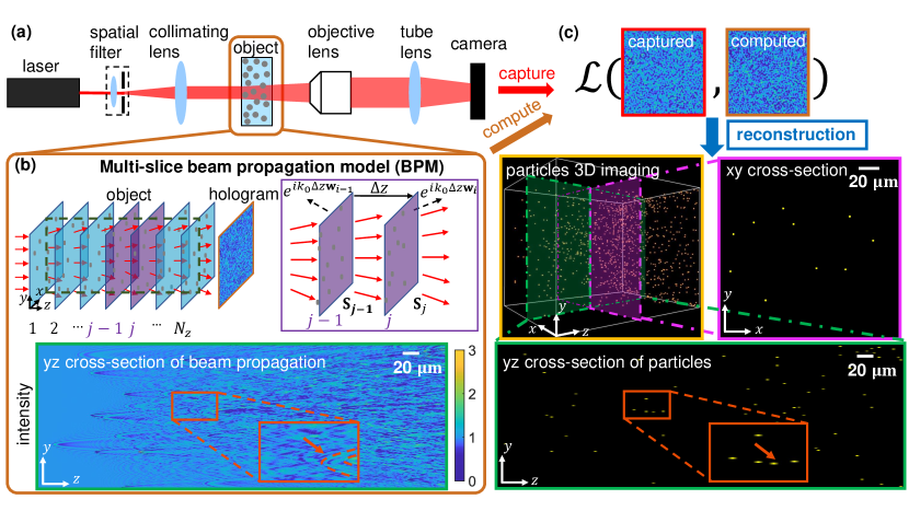
Our imaging geometry is shown in Fig. 1(a). A plane wave passes through a particle volume and the interference pattern resulting from the scattered fields are captured as the hologram. This multiple-scattering image-formation process is modeled as,

where $\hat{\mathbf{I}}\in\mathbb{R}^{M}$ denotes the vectorized, BPM computed intensity hologram containing $M$ pixels. $\mathbf{w}\in\mathbb{R}^{N}=\mathbf{n}-n_{0}$ represents the vectorized 3D refractive index contrast distribution that contains $N$ voxels, and is defined by the difference between the particle’s index distribution $\mathbf{n}$ and the constant background index $n_{0}$. The particle’s refractive index is assumed to be real-valued since the absorption is negligible. $\mathbf{S}:\mathbb{R}^{N}\rightarrow\mathbb{C}^{M}$ is the BPM operator that maps the 3D refractive index to the 2D complex field at the sensor plane.

The BPM is computed by a recursive sequence, as illustrated in Fig. 1(b). It approximates the 3D object as $N_{z}$ infinitesimally thin axial planar slices along the optical axis, each modeled as a 2D phase mask separated equally by a uniform medium. The field is then computed by a sequence of diffraction and refraction operations. Specifically, the field exiting the $j\mathrm{th}$ slice $\mathbf{S}_{j}(\mathbf{w})$ is related to the field from the $(j-1)\mathrm{th}$ slice $\mathbf{S}_{j-1}(\mathbf{w})$ by

where the $\mathbf{S}_{j}:\mathbb{R}^{M}\rightarrow\mathbb{C}^{M}$ is the local BPM operator that maps the $j\mathrm{th}$ phase screen $\mathbf{w}_{j}$ to the 2D complex field after the $j$th slice.

The implementation of the BPM requires an initial condition, for which we set the initial field as a constant-valued on-axis plane wave $\mathbf{S}_{0}(\mathbf{w})=\mathbf{1}$.

The diffraction operator for a propagation distance $\Delta z$ is denoted by $\mathbf{H}$ and computed by $\mathbf{H}=\mathbf{F}^{H}\mathrm{diag}(\mathbf{h})\mathbf{F}$, where $\mathbf{F}$ and $\mathbf{F}^{H}$ are the 2D discrete Fourier and inverse Fourier transform matrices respectively, $\large{\cdot}^{H}$ denotes matrix Hermitian transpose, $\mathrm{diag}(\mathbf{h})$ is a diagonal matrix formed by the vector $\mathbf{h}$ as the main diagonal and is implemented by element-wise multiplication, and $\mathbf{h}$ represents the vectorized 2D angular spectrum transfer function $h(p,q)$:

where $p,q$ index the 2D wave vector in the $k$-space, $k=k_{0}n_{0}$ is the wave-number in the background medium, $k_{0}={2\pi}/{\lambda_{0}}$, $\lambda_{0}$ is the wavelength in vacuum, and $\Delta k$ is the sampling interval in the $k$-space. $\mathcal{P}$ represents the low-pass filter due to the evanescent cutoff.

The refraction operator is implemented by element-wise multiplications between the diffracted field and the accumulated phase $\mathbf{p}_{j}(\mathbf{w}_{j})=e^{jk_{0}\Delta z\mathbf{w}_{j}}$, where $\mathbf{w}_{j}$ denotes the discretized 2D refractive index map in the $j\mathrm{th}$ slice.

The hologram is the intensity of the exit field from the last slice at $N_{z}$ low-pass filtered by the pupil function of the imaging system.

The computation of the BPM thus requires implementing Eq. (2) $N_{z}$ times. The computational complexity of the BPM is $O(N\mathrm{log}(N_{x}N_{y}))$, as set approximately by $2N_{z}$ times evaluations of 2D FFT, where the total number of object voxels is $N=N_{x}N_{y}N_{z}$, and $N_{x}$ and $N_{y}$ are the number of pixels in the $x$ and $y$ directions, respectively. For comparison, the computational complexity of the Born series model is $O(N_{z}N\mathrm{log}(N_{x}N_{y}))$ [9]. Thus, the BPM reduces the computational complexity by $N_{z}$ times, which becomes significant when the object depth is large.

To illustrate the multiple scattering effects modeled by the BPM, we show an example $yz$ cross-section of the intensity distribution computed from a particle volume in Fig. 1(b). In the zoom-in region, complex interference patterns are visible due to multiple particles in the close proximity, which introduces strong multiple scattering effects [22].

We first validate the forward model accuracy by comparing the BPM-computed holograms with experimental measurements. In practice, we assess the accuracy based on analyzing the intensity statistics under different scattering conditions, since the ground-truth particle positions in the experiments are not known.

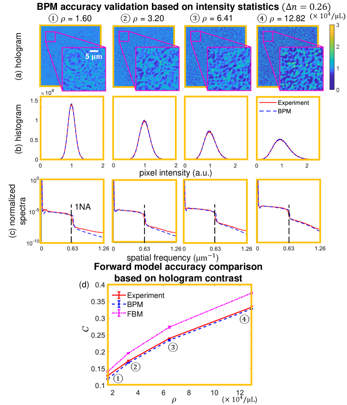
We perform simulations using parameters that match with the experiments. More details about the experiments are provided in Supplementary material. Holograms are computed at four particle densities $\rho$, including $1.60,3.20,6.41,12.82\times 10^{4}/\upmu\mathrm{L}$, corresponding to $250,500,1000,2000$ particles in a $176.64\times 176.64\times 500~{}\upmu\mathrm{m}^{3}$ volume. $1~{}\upmu\mathrm{m}$ particles are randomly placed in 3D positions. The refractive index of the particle $n$ and the background medium (water) $n_{0}$ is 1.59 and 1.33, respectively, and the contrast is $\Delta n=0.26$. To simulate 3D refractive index contrast distribution $\mathbf{w}$, the voxels inside the particles are assigned with the constant $\Delta n$, and the rest of the background voxels are assigned with zero. The lateral sampling size $\Delta x,\Delta y$ are both $0.1725\upmu\mathrm{m}$, and the axial sampling size $\Delta z$ is $\lambda/16=0.0297\upmu\mathrm{m}$, where $\lambda=\lambda_{0}/n_{0}$ and $\lambda_{0}=0.632\upmu\mathrm{m}$. The resulting object size in our forward model is $1024\times 1024\times 16840$ voxels. Example computed holograms at four particle densities are shown in Fig. 2(a). As expected, characteristic fringe patterns from individual particles are still visible at the lowest density case. As the density increases, the holograms gradually become partially developed speckle patterns.

First, we analyze the BPM’s accuracy by comparing the histograms of the computed hologram with the captured hologram at each particle density. As shown in Fig. 2(b), the histograms match well at all four densities.

Next, we assess the BPM’s accuracy in the spatial frequency domain. We calculate the normalized spectra of the computed and captured holograms. As shown in Fig. 2(c), the frequency components of the computed holograms closely match with the experimental measurements within the NA of the imaging system.

Finally, we compare the accuracy of the BPM and FBM based on the hologram contrast $\mathcal{C}=\frac{\sigma}{\mu}$, where $\sigma$ and $\mu$ are the standard deviation and mean of the hologram, respectively.

Briefly, the FBM is a linear model that assumes a weakly scattering object, and the resulting scattered field is linearly related to the scattering potential $V(x,y,z)=\frac{1}{4\pi}k_{0}^{2}[n(x,y,z)^{2}-n_{0}^{2}]$. Given the plane-wave incident field $U_{in}(x,y,z)=e^{in_{0}k_{0}z}$, the total field $U_{\text{FBM}}$ can be approximated as

where the Green’s function $G(r)={\exp(ik_{0}n_{0}r)}/{r}$, $n(x,y,z)$ is the refractive index at location $(x,y,z)$ and $r=\sqrt{x^{2}+y^{2}+z^{2}}$ [5]. The FBM-estimated hologram is $I_{\text{FBM}}=|U_{\text{FBM}}|^{2}$. To perform the computation, the 3D volume is first discretized with voxels in size $\Delta x\times\Delta y\times\Delta z$. In our simulation, $\Delta x=\Delta y=0.1725\upmu\mathrm{m}$ and $\Delta z=\lambda/16$. The scattering potential is calculated as $\frac{1}{4\pi}k_{0}^{2}\Delta x\Delta y\Delta z(n^{2}-n_{0}^{2})$ for voxels within the particle, and is zero for the rest of the voxels. To compute the scattered field, we treat the discretized volume as a series of 2D slabs. The scattered field from a given slab can be efficiently calculated by first multiplying the incident field at the given depth with the scattering potential of the slab and then convolve with the Green’s function implemented with the fast Fourier transform (FFT)-based algorithm. The total field $U_{\text{FBM}}$ is obtained by summing the incident field at the hologram plane and the total scattered field from all the slabs.

As shown in Fig. 2(d), the contrast from the BPM-computed holograms agree well with the experiments. The BPM slightly under-estimates the contrast. A possible reason is that the BPM approximates the multiple forward scattering by computing the complex field slice-by-slice but ignores backscattering. As a result, the BPM may slightly under-estimates the high frequency information, which reduces the contrast in the calculated holograms. As a comparison, the contrast from the FBM-computed holograms are consistently higher than the experimental data. The contrast discrepancy increases as the particle density. At the highest density, the discrepancy for the BPM is 0.0048, whereas the FBM is 0.0422, representing a $9\times$ improvement by the BPM.

Overall, these studies show that the BPM can accurately model multiple scattering in a dense 3D particle field and significantly outperforms the single-scattering model.

The BPM accuracy is primarily influenced by the axial sampling distance $\Delta z$ and the scattering strength of the 3D object. In the following, we quantitatively evaluate the model accuracy under different axial sampling and scattering conditions (by changing the particle density $\rho$ and refractive index contrast $\Delta n$), while fixing the lateral sampling $\Delta x=\Delta y=0.1725\upmu\mathrm{m}$.

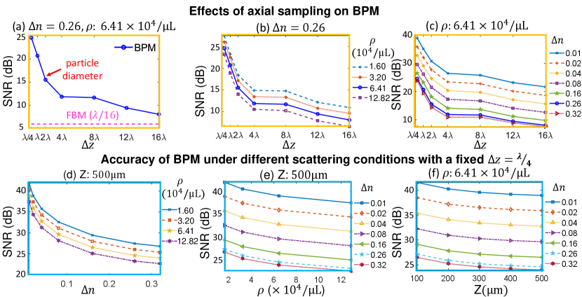
In Fig. 3(a), the accuracy of BPM is plotted for different $\Delta z$ under the same scattering condition. We compare the holograms computed with different $\Delta z$ with the reference $\hat{\mathbf{I}}_{0}$ using $\Delta z=\lambda/16$. The difference is quantified by the signal-to-noise ratio (SNR), $\mathrm{SNR}=10\log_{10}\frac{\|\hat{\mathbf{I}}_{0}\|_{2}}{\|\hat{\mathbf{I}}_{0}-\mathbf{\hat{I}}\|_{2}}$, where $\hat{\mathbf{I}}$ is the computed hologram with axial down-sampling. The accuracy of the BPM drops rapidly when $\Delta z$ is smaller than the particle diameter ($1\upmu\mathrm{m}$) and reduces slowly as $\Delta z$ further increases. This indicates that to accurately compute the inner-particle multiple scattering using the BPM, dense axial sampling is generally needed. Nevertheless, even under coarse axial sampling up to $\Delta z=16\lambda$, the BPM is still more accurate than the FBM computed with the reference dense axial sampling $\Delta z=\lambda/16$.

Next, we study the BPM’s accuracy for different $\Delta z$ for different particle densities $\rho$ and refractive index contrasts $\Delta n$ (Fig. 3(b-c)). Our study shows that the shape of the curve remain the same for different scattering conditions, which suggests that it is only determined by the sampling distance $\Delta z$.

Next, we study how the scattering strength affects the BPM’s accuracy for a fixed $\Delta z=\lambda/4$. We compute holograms at different particle densities $\rho$, refractive index contrasts $\Delta n$, and volume thicknesses $Z$. We then compare these holograms with the corresponding reference ($\Delta z=\lambda/16$). The results are summarized in Fig. 3(d-f). In general, the accuracy decreases as the scattering becomes stronger. The SNR is found to satisfy the following scaling law:

where we define a scaling parameter $A(\Delta z)$ to describe the effects of $\Delta z$ whose values are proportional to that shown in Fig. 3(a). $X,Y,Z$ are the lateral and axial sizes of the object volume and $P$ is the total number of particles. Intuitively, Eq. (13) shows that the SNR is approximately inversely proportional to the total scattering potential $V$ (where $V=\frac{k_{0}^{2}}{3}R^{3}(n^{2}-n_{0}^{2})P$, $n$ is the refractive index of the particles, $R=0.5\upmu\mathrm{m}$ is the radius of the particles) of the particle volume.

Given the high accuracy of the BPM model validated in Sec. 3, we next quantify the accuracy of our reconstruction algorithm in simulation. To implement the reconstruction algorithm, we first select a suitable $\Delta z$. Due to memory limitations, it is not feasible to perform reconstructions using the same dense $\Delta z=\lambda/16$ as the forward simulation. Based on our quantitative study in Fig. 3, we select $\Delta z=6.2\lambda$ for all the reconstructions, which balances the model accuracy and computational cost. The corresponding object volume contains around 177 million voxels.

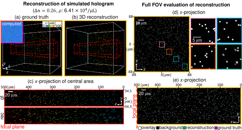
In Fig. 4(a), we simulated a hologram from a particle field ($\rho=6.41\times 10^{4}/\upmu\mathrm{L},\Delta n=0.26$, particle diameter:$1\upmu\mathrm{m}$) using the densely sampled BPM model ($\Delta z=\lambda/16$). The 3D reconstruction result is visualized in Fig. 4(b). For better visualization, we show the $x$-projection of the central $69\times 69\times 500\upmu\mathrm{m}^{3}$ region in Fig. 4(c). As expected, the reconstructed particles are elongated along the $z$-axis due to the missing cone problem. To further evaluate the reconstruction, we extracted the centroids of the reconstructed particles and then overlay them onto the ground-truth. The $z$- and $x$-projections are shown in Fig. 4(d-e). As shown in the $z$-projection, the reconstruction errors mostly occurred in the peripheral FOV region. Further inspecting the the $x$-projection, the localized centroids agree well with the ground truth.

To further quantify the reconstruction accuracy, we repeat the simulation at seven different refractive index contrasts and four different particle densities. We then use Jaccard index (JI), lateral root mean square error (RMSE), and axial RMSE for quantification [24]:

where TP, FP, and FN denote the number of true positive, false positive, and false negative particles, respectively, $\delta x,\delta y,$ and $\delta z$ measure the distance between the centroids of the reconstructed and the matching ground-truth particle, and $B$ is the set of all TP particles, see more details in Supplementary material.

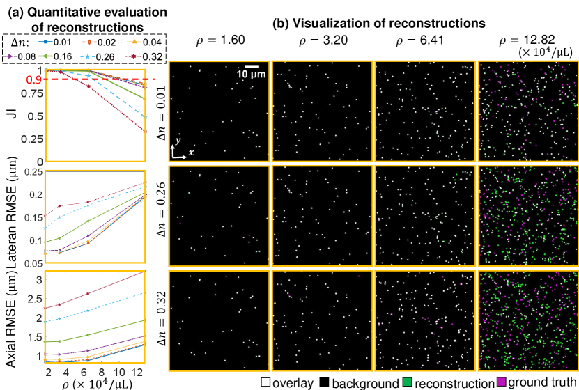
As shown in Fig. 5(a), our method achieves JI > 0.9 for imaging particles at densities $\rho\leq 6.41\times 10^{4}/\upmu\mathrm{L}$ (1000 particles in the $176.74\times 176.74\times 500\upmu\mathrm{m}^{3}$ volume) with $\Delta n=0.26$. Our method also achieves localization accuracy better than the diffraction limit. The lateral RMSE is less than 0.25$\upmu\mathrm{m}$ and the axial RMSE is less than 3.5$\upmu\mathrm{m}$ in all cases. Figure 5(b) shows representative $z$-projections of the centorids overlaid onto the ground-truth for the central $69\times 69\times 500\upmu\mathrm{m}^{3}$ region. These results show that our method performs well for particle densities as high as $6.41\times 10^{4}/\upmu\mathrm{L}$ and refractive index contrast as high as 0.32.

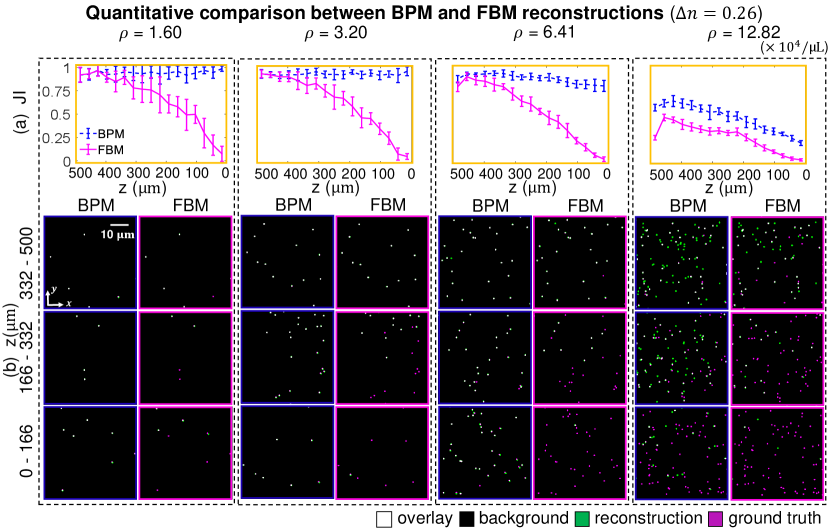
Next, we quantify the improvement of our multiple-scattering BPM model as compared to the single-scattering FBM model. To do so, we performed reconstructions using the compressive holography algorithm that uses the FBM forward model and a total variation (TV) regularization to enforce sparsity [6, 7]. In Fig. 6, we compare results across four different particle densities with $\Delta n=0.26$. To quantify the depth-dependent reconstruction accuracy, we calculated JI by dividing the entire depth into 17 segments and then calculating JI for each segment. The depth-wise JIs under different scattering densities are shown in Fig. 6(a). The results show that the BPM-based algorithm consistently detects the particles across all the depths for particle densities $\rho\leq 6.41\times 10^{4}/\upmu\mathrm{L}$. In contrast, the FBM-based algorithm suffers from rapid degradation as the depth increases. In particular, when the depth is around $500\upmu\mathrm{m}$, the JI of BPM is $>34$ times higher than the FBM when $\rho\leq 6.41\times 10^{4}/\upmu\mathrm{L}$. Representative $z$-projections of the reconstructed centroids overlaid onto the ground truth across different depths are shown in Fig. 6(b) for the central $69\times 69\times 500\upmu\mathrm{m}^{3}$ region. These results highlight that our multiple-scattering algorithm significantly outperforms the traditional single-scattering method, in particular for reconstructing particles at deep depths.

We demonstrate our reconstruction algorithm on experimentally captured holograms at 4 different densities. In Fig. 7, 3D visualizations of example reconstruction results are shown in depth-color coded 3D renderings and $x$- and $z$-projections. The axial elongations are visible in all cases, which are resulted from the missing spatial frequency information limited by the single-view holographic measurement.

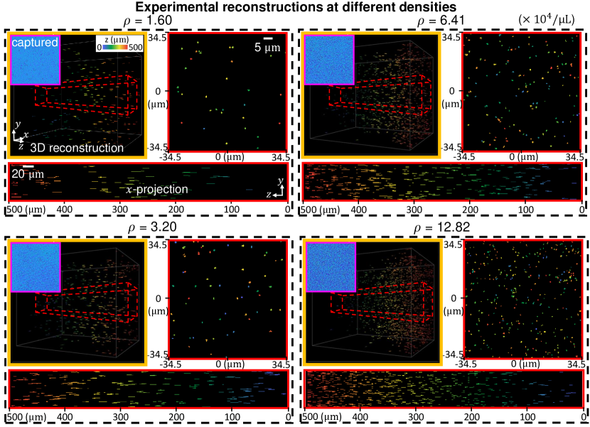
We further observe that more particles are reconstructed at the depths closer to the hologram plane. This is expected since, for particles closer to the hologram plane, a greater amount of scattered information are captured by the finite-sized image sensor.

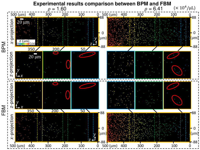
Finally, we compare our method with the FBM algorithm in Fig. 8. Similar to our observations in the simulation, the BPM algorithm can better reconstruct particles at deeper depths than the FBM algorithm, as highlighted by the $x$- and $z$-projections for different depth regions.

References

- [1] F. C. Cheong, B. S. R. Dreyfus, J. Amato-Grill, K. Xiao, L. Dixon, and D. G. Grier, “Flow visualization and flow cytometry with holographic video microscopy,” \JournalTitleOptics express 17, 13071–13079 (2009).
- [2] I. Moon, M. Daneshpanah, B. Javidi, and A. Stern, “Automated three-dimensional identification and tracking of micro/nanobiological organisms by computational holographic microscopy,” \JournalTitleProceedings of the IEEE 97, 990–1010 (2009).
- [3] T.-W. Su, L. Xue, and A. Ozcan, “High-throughput lensfree 3d tracking of human sperms reveals rare statistics of helical trajectories,” \JournalTitleProceedings of the National Academy of Sciences 109, 16018–16022 (2012).
- [4] L. Tian, N. Loomis, J. A. Domínguez-Caballero, and G. Barbastathis, “Quantitative measurement of size and three-dimensional position of fast-moving bubbles in air-water mixture flows using digital holography,” \JournalTitleApplied optics 49, 1549–1554 (2010).
- [5] M. Born and E. Wolf, Principles of Optics: Electromagnetic Theory of Propagation, Interference and Diffraction of Light (Cambridge University Press, 1999), 7th ed.
- [6] D. J. Brady, K. Choi, D. L. Marks, R. Horisaki, and S. Lim, “Compressive holography,” \JournalTitleOptics express 17, 13040–13049 (2009).
- [7] W. Chen, L. Tian, S. Rehman, Z. Zhang, H. P. Lee, and G. Barbastathis, “Empirical concentration bounds for compressive holographic bubble imaging based on a mie scattering model,” \JournalTitleOptics express 23, 4715–4725 (2015).
- [8] U. S. Kamilov, D. Liu, H. Mansour, and P. T. Boufounos, “A recursive born approach to nonlinear inverse scattering,” \JournalTitleIEEE Signal Processing Letters 23, 1052–1056 (2016).
- [9] W. Tahir, U. S. Kamilov, and L. Tian, “Holographic particle localization under multiple scattering,” \JournalTitleAdvanced Photonics 1, 036003 (2019).
- [10] P. M. Van Den Berg and R. E. Kleinman, “A contrast source inversion method,” \JournalTitleInverse problems 13, 1607 (1997).
- [11] B. T. Draine and P. J. Flatau, “Discrete-dipole approximation for scattering calculations,” \JournalTitleJosa a 11, 1491–1499 (1994).
- [12] K. D. Unger, P. C. Chaumet, G. Maire, A. Sentenac, and K. Belkebir, “Versatile inversion tool for phaseless optical diffraction tomography,” \JournalTitleJOSA A 36, C1–C8 (2019).
- [13] E. Mudry, P. C. Chaumet, K. Belkebir, and A. Sentenac, “Electromagnetic wave imaging of three-dimensional targets using a hybrid iterative inversion method,” \JournalTitleInverse Problems 28, 065007 (2012).
- [14] T. Zhang, C. Godavarthi, P. C. Chaumet, G. Maire, H. Giovannini, A. Talneau, M. Allain, K. Belkebir, and A. Sentenac, “Far-field diffraction microscopy at /10 resolution,” \JournalTitleOptica 3, 609–612 (2016).
- [15] H.-Y. Liu, D. Liu, H. Mansour, P. T. Boufounos, L. Waller, and U. S. Kamilov, “Seagle: Sparsity-driven image reconstruction under multiple scattering,” \JournalTitleIEEE Transactions on Computational Imaging 4, 73–86 (2017).
- [16] U. S. Kamilov, I. N. Papadopoulos, M. H. Shoreh, A. Goy, C. Vonesch, M. Unser, and D. Psaltis, “Optical tomographic image reconstruction based on beam propagation and sparse regularization,” \JournalTitleIEEE Transactions on Computational Imaging 2, 59–70 (2016).
- [17] L. Tian and L. Waller, “3d intensity and phase imaging from light field measurements in an led array microscope,” \JournalTitleoptica 2, 104–111 (2015).
- [18] S. Chowdhury, M. Chen, R. Eckert, D. Ren, F. Wu, N. Repina, and L. Waller, “High-resolution 3d refractive index microscopy of multiple-scattering samples from intensity images,” \JournalTitleOptica 6, 1211–1219 (2019).
- [19] M. Chen, D. Ren, H.-Y. Liu, S. Chowdhury, and L. Waller, “Multi-layer born multiple-scattering model for 3d phase microscopy,” \JournalTitleOptica 7, 394–403 (2020).
- [20] K. Tam and V. Perez-Mendez, “Tomographical imaging with limited-angle input,” \JournalTitleJOSA 71, 582–592 (1981).
- [21] J. Lim, K. Lee, K. H. Jin, S. Shin, S. Lee, Y. Park, and J. C. Ye, “Comparative study of iterative reconstruction algorithms for missing cone problems in optical diffraction tomography,” \JournalTitleOptics express 23, 16933–16948 (2015).
- [22] J. Lim, A. Goy, M. H. Shoreh, M. Unser, and D. Psaltis, “Learning tomography assessed using mie theory,” \JournalTitlePhysical Review Applied 9, 034027 (2018).
- [23] A. Beck and M. Teboulle, “A fast iterative shrinkage-thresholding algorithm for linear inverse problems,” \JournalTitleSIAM journal on imaging sciences 2, 183–202 (2009).
- [24] D. Sage, T.-A. Pham, H. Babcock, T. Lukes, T. Pengo, J. Chao, R. Velmurugan, A. Herbert, A. Agrawal, S. Colabrese, A. Wheeler, A. Archetti, B. Rieger, R. Ober, G. M. Hagen, J.-B. Sibarita, J. Ries, R. Henriques, M. Unser, and S. Holden, “Super-resolution fight club: assessment of 2d and 3d single-molecule localization microscopy software,” \JournalTitleNature methods 16, 387–395 (2019).
- [25] Z. Wu, Y. Sun, A. Matlock, J. Liu, L. Tian, and U. S. Kamilov, “Simba: Scalable inversion in optical tomography using deep denoising priors,” \JournalTitleIEEE Journal of Selected Topics in Signal Processing 14, 1163–1175 (2020).
- [26] A. Matlock and L. Tian, “Physical model simulator-trained neural network for computational 3d phase imaging of multiple-scattering samples,” \JournalTitlearXiv preprint arXiv:2103.15795 (2021).
- [27] H. Wang, W. Tahir, J. Zhu, and L. Tian, “Large-scale-3d-holographic-imaging-with-beam-propagation,” https://github.com/bu-cisl/Large-Scale-3D-Holographic-Imaging-with-Beam-Propagation. GitHub (2021).