Large-scale non-Gaussian mass function and halo bias: tests on N-body simulations
Abstract
The description of the abundance and clustering of halos for non-Gaussian initial conditions has recently received renewed interest, motivated by the forthcoming large galaxy and cluster surveys, which can potentially yield constraints of order unity on the non-Gaussianity parameter . We present tests on N-body simulations of analytical formulae describing the halo abundance and clustering for non-Gaussian initial conditions. We calibrate the analytic non-Gaussian mass function of Matarrese et al. (2000) and LoVerde et al. (2008) and the analytic description of clustering of halos for non-Gaussian initial conditions on N-body simulations. We find excellent agreement between the simulations and the analytic predictions if we make the corrections and where , in the density threshold for gravitational collapse and in the non-Gaussian fractional correction to the halo bias, respectively. We discuss the implications of this correction on present and forecasted primordial non-Gaussianity constraints. We confirm that the non-Gaussian halo bias offers a robust and highly competitive test of primordial non-Gaussianity.
keywords:
methods: statistical, -body simulations–cosmology: theory, large-scale structure of universe galaxies: clusters: general – galaxies: halos1 Introduction
Constraining primordial non-Gaussianity offers a powerful test of the generation mechanism of cosmological perturbations in the early universe. While standard single-field models of slow-roll inflation lead to small departures from Gaussianity, non-standard scenarios allow for a larger level of non-Gaussianity (Bartolo et al. (2004) and references therein). The standard observables to constrain non-Gaussianity are the Cosmic Microwave Background (CMB) and the Large Scale Structure (LSS) of the Universe. A powerful technique is based on the abundance (Matarrese et al., 2000; Verde et al., 2001; LoVerde et al., 2008; Koyama et al., 1999; Robinson & Baker, 2000; Robinson et al., 2000) and clustering (Grinstein & Wise, 1986; Matarrese et al., 1986; Lucchin et al., 1988) of rare events, such as dark matter density peaks, as they trace the tail of the underlying matter distribution. Theoretical predictions on various observational aspects of non-Gaussianity have been extensively tested against N-body simulations, leading to different and sometimes conflicting results (Kang et al., 2007; Grossi et al., 2007; Dalal et al., 2007; Desjacques et al., 2008; Pillepich et al., 2008).
Dalal et al. (2007) and Matarrese & Verde (2008) showed that primordial non-Gaussianity affects the clustering of dark matter halos inducing a scale-dependent bias on large scales. Not only this effect has been already exploited to place stringent constraints on non-Gaussianity (Slosar et al., 2008; Afshordi & Tolley, 2008), but also it is particularly promising for constraining non-Gaussianity from future surveys, which will provide a large sample of galaxy clusters over a volume comparable to the horizon size (e.g., DES, PanSTARRS, BOSS, LSST, ADEPT, EUCLID) (Dalal et al., 2007; Carbone et al., 2008; Afshordi & Tolley, 2008; Seljak, 2008). Bartolo et al. (2005) showed that even for small primordial non-Gaussianities, the evolution of perturbations on super-Hubble scales yields extra contributions. The amplitude of these contributions is comparable to the forecasted errors of some planned surveys, opening up the possibility of measuring them.
In light of this, it is important to use N-body experiments to test the validity of theoretical predictions for halo-bias in non-Gaussian framework. Indeed, all proposed analytic biasing expressions have been derived in the extended Press-Schechter framework which assumes spherical collapse dynamics, sharp k-space filtering and Gaussian initial conditions. The validity of the extrapolation of the extended Press-Schechter approach to the non-Gaussian case can be tested independently by considering also the halo mass function. It is thus also important to test and calibrate on N-body simulations the predictions of the non-Gaussian halo mass function (Kang et al., 2007; Grossi et al., 2007; Dalal et al., 2007) and of the non-Gaussian halo bias simultaneously. This is what we set out to do here.
In this paper we start by reviewing the analytic predictions for the Gaussian and non-Gaussian halo abundance and clustering (§2). In §3 we describe the numerical simulations with Gaussian and non-Gaussian initial conditions. In §4 we present the test for the non-Gaussian mass function. In §5 and 6 we test the analytic predictions of Gaussian and non-Gaussian large scale bias against N-body simulations. In §7 we compare our results with the literature. Finally, we conclude in §8.
2 Formulation of the non-Gaussian halo abundance and clustering
Deviations from Gaussian initial conditions are commonly parameterized in terms of the dimensionless parameter (Salopek & Bond, 1990; Gangui et al., 1994; Verde et al., 2000; Komatsu & Spergel, 2001):
| (1) |
where denotes the gravitational potential and is a Gaussian random field. As noted by e.g., LoVerde et al. (2008), Afshordi & Tolley (2008) and Pillepich et al. (2008), different authors use different conventions. Here denotes Bardeen’s gauge-invariant potential which, on sub-Hubble scales, reduces to the usual Newtonian peculiar gravitational potential but with a negative sign. In addition, there are two conventions for normalizing Eq. (1): the LSS and the CMB one. In the LSS convention is linearly extrapolated at . In the present paper we use this convention. In the CMB convention is instead primordial: thus , where denotes the linear growth suppression factor in non Einstein-de-Sitter Universes.
2.1 Formulation of the non-Gaussian mass function: Extended Press-Schechter approach
In the Press-Schechter framework, one considers the density contrast field evaluated at some early time, far before any scale of interest has approached the nonlinear regime, but extrapolated to the present day using linear perturbation theory. Then one considers the height of the critical density threshold as a function of time. In that way, the collapse of a halo at redshift corresponds to the density fluctuation crossing a barrier of height , where (this is an equality only in an Einstein de Sitter Universe); we use , . We should recall here that, even in linear theory, the normalized skewness of the density field, , depends on redshift , however in the Press-Schechter framework one should use the linear , in what follows . Note also that in general the skewness can be written as , where denotes the skewness in units of , care must be exercised in the interpretation of : if is that of the density field linearly extrapolated at , must be the LSS one and not the CMB one.
Generalization of the mass function to non-Gaussian initial conditions within the Press-Shechter formalism has been presented in Matarrese et al. (2000); LoVerde et al. (2008). Both references start by computing an expression for the non-Gaussian probability density function of the smoothed dark matter density field, then obtain the level excursion probability. In the Press-Shechter approach the mass derivative of the level excursion probability is the key ingredient to obtain the mass function expression and is the term that gets modified in the presence of primordial non-Gaussianity. In this derivation, several approximations are made. Both approaches assume that deviations from Gaussianity are small.
Matarrese et al. (2000) use first the saddle-point approximation to compute the level excursion probability and then truncate the resulting expression at the skewness. They obtain 111We correct here a typo in Eq. (68) of Matarrese et al. (2000), where should be .:
where denotes the rms value of the density field, the subscript denotes that the density field has been smoothed on a scale corresponding to , and .
LoVerde et al. (2008) instead first approximate the probability density function using the Edgeworth expansion, then perform the integral of the level excursion probability exactly on the first few terms of the expansion. They obtain:
Note that in the limit of small non-Gaussianity and rare events, the ratio of the non-Gaussian mass function to the Gaussian one for both expressions reduces to:
| (4) |
It is important to bear in mind that in Eqs. (2.1)-(2.1), the redshift dependence is enclosed only in (and not in ). In the spirit of the “CMB” convention instead, where the gravitational potential is normalized deep in the matter era, one should make sure that all the relevant quantities are correctly extrapolated linearly at , keeping in mind that the gravitational potential slowly evolves in a non Einstein de Sitter Universe.
The major limitations in both derivations are the assumption of spherical collapse and the sharp -space filtering. In addition, the excursion set improvement on the interpretation of the original Press-Shechter swindle, suggests that this derivation relies on the random-phase hypothesis Sheth (1998), which is clearly not satisfied for non-Gaussian initial conditions even for sharp -space filtering.
Verde et al. (2001) and LoVerde et al. (2008) addressed this issue by using the analytical approach to compute the fractional non-Gaussian correction to the Gaussian mass function , and used the Sheth & Tormen (1999) mass function to model the Gaussian mass function. This approach is potentially promising, but needs to be calibrated on numerical experiments.
In particular, one may argue that the same correction that in the Gaussian case modifies the collapse threshold and thus the form of the mass function from Press & Schechter (1974) to Sheth et al. (2001) and Sheth & Tormen (2002), may apply to the non-Gaussian correction. In the Gaussian case this is usually referred to as the correction due to ellipsoidal collapse (Lee & Shandarin, 1998). While this interpretation has recently been disputed (see e.g., Robertson et al. (2008)), we will maintain the same nomenclature here. For rare events, high peaks () and small , this is equivalent to lower by a factor with .
In summary we propose that the non-Gaussian mass function should be re-written in terms of the Gaussian one –given by tested fits to simulations e.g., Sheth & Tormen (1999); Reed et al. (2003); Warren et al. (2006); Jenkins et al. (2001)–, multiplied by a non-Gaussian correction factor:
| (5) |
where takes two different forms in the Matarrese et al. (2000) and LoVerde et al. (2008) approximations. For the Matarrese et al. (2000) case 222We correct here a typo in Eq. (3) of Grossi et al. (2007) where the exponential part was missing.
| (6) | |||
and for the LoVerde et al. (2008) case:
| (7) | |||
where denotes the critical density for ellipsoidal collapse, which for high peaks is with .
2.2 Formulation of the non-Gaussian large scale halo bias
For the case of “local” primordial non-Gaussianity Eq. (1), the analytical expression for the large-scale non-Gaussian bias has been derived in five different ways, obtaining always basically the same result. Dalal et al. (2007) considered the Laplacian of in the vicinity of rare, high peaks, considering that the resulting is proportional to the peaks overdensity; they also generalized to local non-Gaussianity the Kaiser (1984) argument of high-peaks bias in order to derive its non-Gaussian version. Matarrese & Verde (2008) derived the halo bias formula in general non-Gaussian cases specified by an expression for the bispectrum. Slosar et al. (2008) adopted the peak-background split approach (Cole & Kaiser, 1989) for the local non-Gaussian case, showing that the resulting expression relies on the universality of the mass function. Afshordi & Tolley (2008) instead interpreted non-Gaussianity as a modification of the critical density for collapse, in the framework of ellipsoidal collapse. Finally, McDonald (2008) used a renormalized perturbation theory approach to consider at the same time non-linear bias, second-order gravitational evolution and local form of non-Gaussianity. It is encouraging that these different approaches yield a consistent result for the correction to the Gaussian Lagrangian halo bias :
| (8) |
where encloses the scale and halo mass dependence –see e.g., Eq. (13) and Fig. 3 of Matarrese & Verde (2008)–. Also in this case the density field is the one extrapolated linearly at , and does not depend on redshift.
Making the standard assumption that halos move coherently with the underlying dark matter, the Lagrangian bias is related to the Eulerian one as .
The approximations used to derive this equation are Press-Schechter (Press & Schechter, 1974) approach, linear bias, small non-Gaussianity, and in most cases spherical collapse and identification of peaks with halos. It is therefore important to test the validity of Eq. (8), with simulations and see if any correction factor needed is indeed due to account for non-spherical collapse. Following the derivation of Matarrese & Verde (2008) we recognize that the correction to the 2-point halo correlation function due to non-Gaussianity (their Eq. (6)) is multiplied by with . In this factor we recognize one Lagrangian Gaussian bias factor to the second power and an extra , which denominator was absorbed in the form factor. Recall that, as discussed in §2.1, for “ellipsoidal collapse” and rare events, the Lagrangian Gaussian bias is corrected as (see Eq. (11) below, for high ). However, the remaining factor is also a Gaussian bias and it should also be corrected by the -factor.
We conclude that the “non-spherical collapse” modifies Eq. (8) to be:
| (9) |
Note that Afshordi & Tolley (2008) arrived to a similar yet not identical expression when considering ellipsoidal collapse, i.e. they suggest that should be substituted by the critical density of Sheth et al. (2001), which in our limit would correspond to use rather than in Eq. (9).
3 N-body simulations
The deviations from Gaussianity we are after become important on very large scales h/Mpc and for massive halos. Therefore, one needs to perform N-body simulations on very large boxes, yet with enough resolution to identify massive virialized structures at different redshifts.
Suitable initial conditions have been set up following the method described in more detail in Grossi et al. (2008) (see also Grossi et al. (2007); Viel et al. (2009)). In brief, a random realization of a Gaussian gravitational potential, , normalized to be the one linearly extrapolated at , is generated in Fourier space, then it is inverse-Fourier transformed back to real space and added to the non-Gaussian term, . The resulting field that is linear and at , is transformed back in Fourier space. We eventually modulate the power-law spectrum using the transfer function and compute the corresponding density field, which we then scale back to the initial conditions redshift (). The corresponding gravitational potential is then used to displace particles according to the Zel’dovich approximation. This method allows one to simulate non-Gaussian models having power spectra which are all consistent with that of the Gaussian case and was already used by Viel et al. (2009).
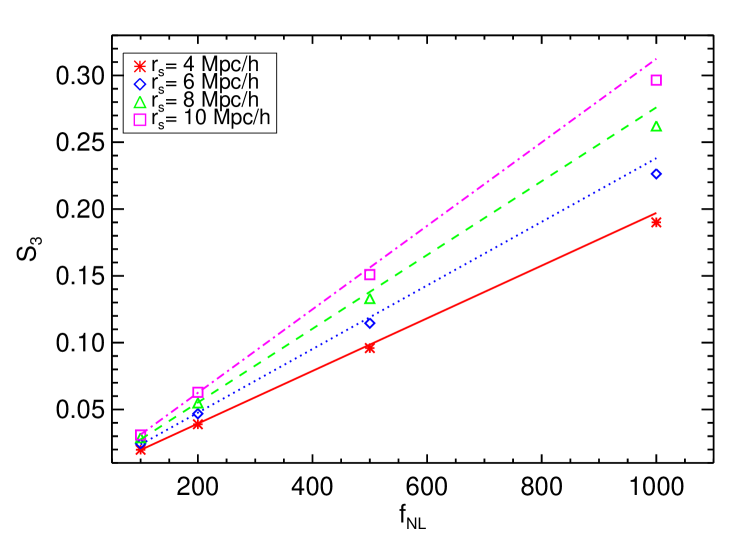
In order to check the reliability of the initial conditions generation, we have performed a specific test: using particles in a box of size 1000 Mpc, primordial density fields (extrapolated linearly at ) were generated and smoothed using spherical top-hat filters of different radii , , , Mpc/. The smoothed skewness was then extracted from the fields and compared to the analytical prediction for , as shown in Figure 1.
The set of simulations used in this work assumes the ‘concordance’ CDM model. We fix the relevant parameters consistently with those derived from the analysis of the WMAP 5-year data (Komatsu et al., 2008): for the matter density parameter, for the contribution to the density parameter, for the Hubble parameter (in units of km s-1 Mpc-1). The initial power spectrum adopts the Cold Dark Matter (CDM) transfer function suggested by Eisenstein & Hu (1999), has a spectral index and is normalized in such a way that . In all experiments, performed using the GADGET-2 numerical code (Springel, 2005), switching off the hydrodynamical part, we consider a box of (1200 Mpc/ with particles: the corresponding particle mass is then . The gravitational force has a Plummer-equivalent softening length of kpc. The runs produced 15 outputs from the initial redshift () to the present time. The 5 simulations consider different amounts of primordial non-Gaussianity, parametrized by the parameter: (i.e. the reference Gaussian case) and . The catalogues of dark matter haloes are extracted from the simulations using the standard friends-of-friends algorithm adopting a linking length of times the mean interparticle distance; only objects with at least particles are considered.
We thus measure the halo bias in the simulations as
| (10) |
where denotes the cross-power spectrum of dark matter with halos of mass at scale , and for the simulation snapshot at redshift . Similarly denotes the dark matter power spectrum. Here and hereafter the subscript denotes quantities measured from the simulation.
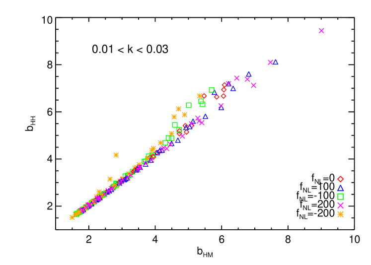
In principle, the quantity one is interested in would be the bias of the halo power spectrum , but is a less noisy quantity (the shot noise of the finite number of halos is greatly suppressed in the estimate of ). The quantity is not guaranteed to be identical to if bias has a stochastic component that does not correlate with the matter density field. In Fig. 2 we show that this is not the case and that there is good agreement on large scales between and , justifying using the less noisy as an estimator for .
3.1 Comparison with independent simulations
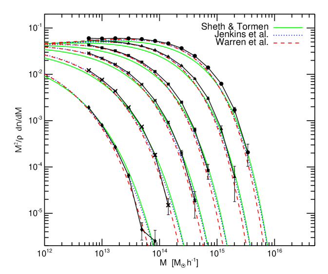
In Fig. 3 we show the mass function extracted from our Gaussian simulations at the following redshifts: and . We also show three different theoretical predictions (also calibrated on N-body simulations): Sheth & Tormen (1999); Jenkins et al. (2001); Warren et al. (2006), solid, dotted and dashed lines respectively. There is good agreement even at high redshift.
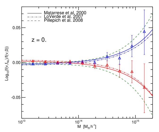
Several groups recently presented N-body simulations, aiming at quantifying the effect of the non Gaussian initial conditions on the halo mass function (Desjacques et al., 2008; Pillepich et al., 2008). All these results are obtained for similar cosmological parameters, so that we can compare estimates derived from all the simulations directly. By comparing the results for the individual simulations at , and in Figures 4, 5 we demonstrate that these results are in agreement among the different groups, once the values are suitably converted to the same convention. Although all simulations use boxes of Giga parsec scales to explore the effect of non-Gaussian initial conditions at the high mass end, the statistical errors at the scale of massive clusters are still large. Therefore, we also report the reciprocal of the results obtained for negative so that they appear in the positive part of the plot, to give an intuitive feeling of the noise within the individual simulations.
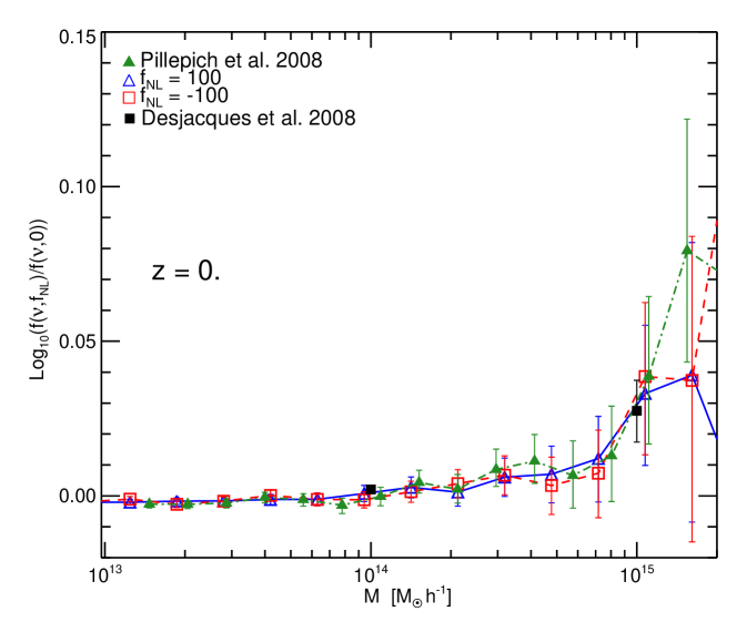
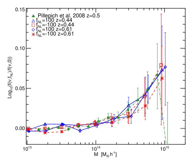
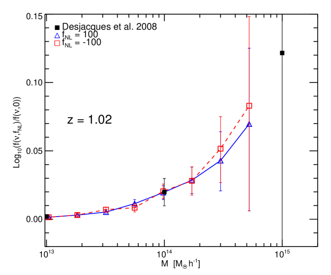
In Figure 4, we show our simulation results for (blue triangles) and for (red squares) at compared with data points from Figure 1 of Desjacques et al. (2008) (black points) at the values of corresponding to , and (as given in their figure caption). Note that, as Desjacques et al. (2008) use in the CMB convention for their simulations, we scaled the points down accordingly by a factor 1.3 to be comparable with our . We also show the results for Pillepich et al. (2008) (green points). Here we again apply the re-scaling as before, as their of would correspond to a of in the LSS notation.
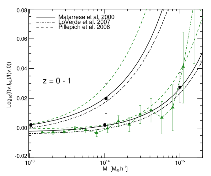
In Figure 5, the left panel shows the results for Pillepich et al. (2008) (green points) at , and our points for the two closest available output times of our simulation ( and ). The right panel shows the comparison at between our points (blue triangles and red squares) and points from Desjacques et al. (2008) (black squares).
¿From this comparison we conclude that there is remarkable agreement between the three independents simulations, highlighting the robustness of the simulations results. The differences visible at some of the highest mass bins are not significant, given the large error bars present.
4 Mass function
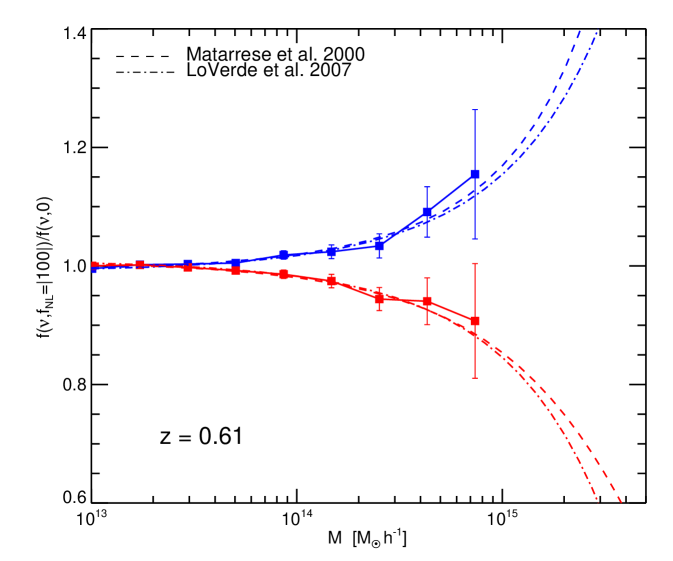
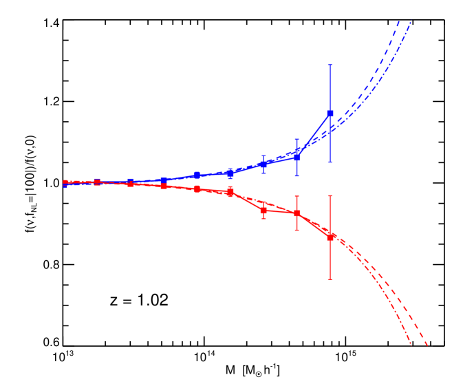
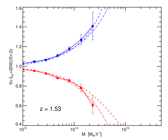
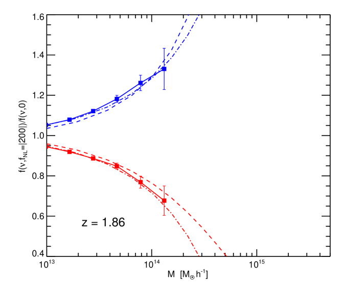
We compare the halo mass function of the non-Gaussian simulations with the theoretical predictions of Eqs. (5), (6) and (7) that is, including our ansatz for the the non-spherical collapse correction: . For clarity we show here the non-Gaussian to Gaussian mass function ratio, i.e. the factor . The comparison between theory and simulations results is shown in Fig. 6 for a few redshift snapshots and for , and in Fig. 7 for for the same redshifts. Dashed lines are the mass function of Matarrese et al. (2000)–Eq. (6) – and dot-dashed lines are that of LoVerde et al. (2008)–Eq. (7)–.
Contrary to Kang et al. (2007) and Dalal et al. (2007), we conclude that both Matarrese et al. (2000) and LoVerde et al. (2008) are good descriptions of the non-Gaussian correction to the mass function, once the correction for non-spherical collapse is included.
Figs. 6 and 7 seem to indicate that LoVerde et al. (2008) may be a better fit for small masses and Matarrese et al. (2000) at high masses. This is not surprising: the Edgeworth expansion works well away from the extreme tails of the distribution (i.e. for moderate ), while the saddle-point-approximation used in Matarrese et al. (2000), is expected to work better at the very tails of the distribution (very high ). We expect that the mass function of Matarrese et al. (2000) will be a better fit at very high masses or larger . This will be further explored in future work.
5 Gaussian halo bias, and the effect of mergers
The large-scale, linear halo Eulerian bias for the Gaussian case is (Mo et al., 1997; Scoccimarro et al., 2001)
| (11) |
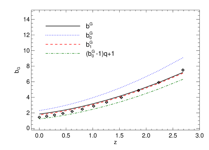
where and , account for non-spherical collapse and are a fit to numerical simulations. Here, denotes the rms value of the dark matter fluctuation field smoothed on a scale corresponding to the Lagrangian radius of the halos of mass ; denotes the halo formation redshift and denotes the halo observation redshift. As we are interested in massive halos, we expect that . As the non-Gaussian halo bias correction is proportional to , the dependence of on whether the selected halos underwent a recent merger (i.e. ) or are old halos (i.e. ) affects the amplitude of the non-Gaussian correction (Slosar et al., 2008; Carbone et al., 2008). Before we trust our simulation to accurately describe the non-Gaussian halo bias we check whether we recover the Gaussian one and whether the linear halo bias approximation is a good description for the scales, redshifts and mass-ranges we are interested in. Gao et al. (2005) show that analytical predictions for the Gaussian halo bias are in reasonable agreement with simulations and that the bias for low-mass halos shows strong dependence on formation time but high mass halos (the ones we are interested in) do not. The halo bias for the Gaussian simulation and the comparison with the theory prediction is shown in Fig. 8. Except for the Gaussian halo bias defined in Efstathiou et al. (1988) and Kaiser (1984) indicated by the dotted (blue) line, the simulated data agree with the theoretical expectations at different redshifts. In particular, in Fig. 8, the black solid line represents the total Gaussian bias of Eq. (11), the dashed (red) line represents the contribution from the first line of Eq. (11), and, finally, the dot-dashed (green) line is . The small difference when using implies that, for the Gaussian halo bias of very massive halos (M⊙), it is reliable to assume that the correction from the “non-spherical collapse” can be encapsulated in the factor in front of .
6 Non-Gaussian halo bias
Eq. (8) shows that the redshift and scale dependence of the non-Gaussian correction can be factorized as a term that depends only on redshift and one that depends only on and . The -dependence is expected to be very weak at large scales ( h/Mpc). Here we will test the mass, scale and redshift dependence of the non-Gaussian halo bias and we calibrate its normalization on the simulations.
In Fig. 9 we show the dependence on halo mass of . We define the quantity
| (12) |
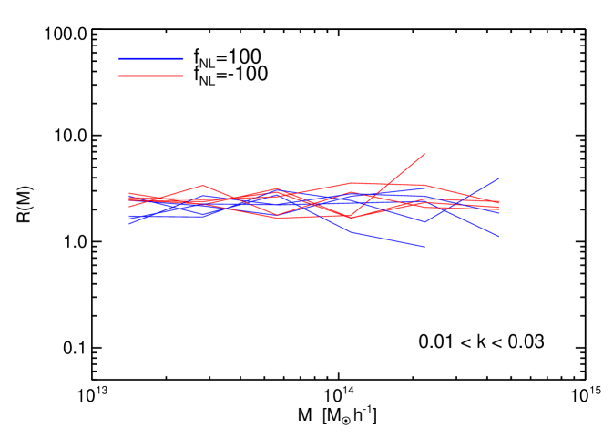
where is given by Eq. (8). To study the mass dependence, we evaluate the theory at fixed mass . We compute the bias from the simulations taking halos in six different mass bins. Fig. 9 includes only scales /Mpc, different lines correspond to different redshift snapshots between and . As expected, there is no noticeable dependence on halo mass.
Having confirmed the expected weak dependence on halo mass for masses and on scales /Mpc, we can study the redshift and scale dependence of , considering halos of different masses above .
The redshift dependence of , is shown in Fig. 10 where and scales /Mpc were used.
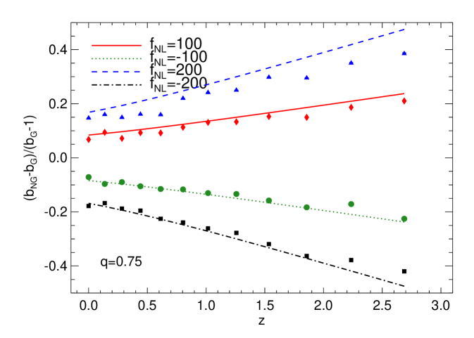
In applying the correction to we have actually corrected , i.e. we have employed the same approximation used for the green dot-dashed line of Fig. 8, giving Eq. (9). Eq.(9) in fact is only the consequence of our correction to the Gaussian halo bias. Note that the approximation we employed here is expected to hold for rare–massive–halos and Fig. 8 shows that this is a good approximation. A detailed study of the dependence of the non-Gaussian halo bias correction on the formation redshift of the halos will be presented elsewhere.
There seems to be an indication that the -correction factor for the large-scale bias correction may slightly depend on the value of : in particular the figure shows that it could be slightly smaller than for large and negative and smaller for large and positive. This is not unexpected: the presence of non-Gaussianity may alter the dynamics of non-spherical collapse (e.g., through tidal forces – see e.g., Desjacques (2008) – or by significantly changing the redshift for collapse with respect to the Gaussian case). At this stage, however, this trend is not highly significant and further study will be left to future work.
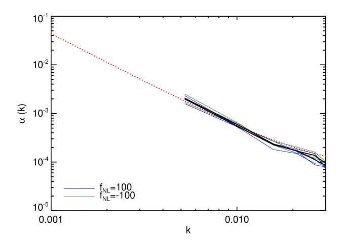
Finally, we show the scale dependence of Eq. (9), , in Fig. 11. The thin lines correspond to different redshifts and the thick black line to their average. The dotted line is the theory prediction with . Note that there is an excellent agreement on the scales of interest, e.g., /Mpc. On smaller scales the effect of non-Gaussianity is very small and the measurement become extremely noisy. These results are in qualitative agreement with the findings of Pillepich et al. (2008).
We conclude that Eq. (9), with , provides a good fit to non-Gaussian simulations.
7 Comparison with previous work
After the discussion of §2, it should be clear that if were used in the theoretical predictions or were not linearly extrapolated to , then any constraints on non-Gaussianity so obtained would have to be re-scaled by a factor . This seems to be the case of some work in the literature. On the other hand the q-correction factor effectively introduces a re-scaling of a factor for the mass function case and for the bias case. It is a coincidence that, for the halo bias, , thus the normalization mistake cancels out with the spherical collapse approximation error. This fortuitous cancellation does not happen to the same level in the mass function , explaining perhaps some of the claimed discrepancy of the simulations with the analytic mass function predictions, and the claimed agreement with the halo bias predictions. Another possible source of inaccuracy would be an inconsistent treatment of the redshft evolution of and (see discussion is §2).
In Fig. 12 we compare our theoretical predictions with the results presented in Pillepich et al. (2008) and Desjacques et al. (2008). The left panel shows our simulation results at for and our theoretical predictions. Additionally we show the fit presented by Pillepich et al. (2008), Eqs. (8) and (9), evaluated for the suitable values of accounting for the different notations for . We also adopt our cosmological parameters when converting to . The right panel shows the simulation results presented in Pillepich et al. (2008) at z=0 and their fitting formula at and . We over plot our theoretical models evaluated for their cosmological parameters and for the corresponding values of . Moreover we add the data points from Desjacques et al. (2008) for and , suitably rescaled by the differences of the value used. The mass function fits of Fig. 12 differ for large masses, in the regime where simulations errors become large; the fits are however consistent given the individual points error-bars.
Our theoretical formulae for the non-Gaussian mass function (Eqs. 5, 6, 7) and for the non-Gaussian halo bias (Eq. 9) are physically motivated expressions that have been tested on N-body simulations. They have the advantage over fitting formulae that they can be more robustly interpolated and extrapolated to cosmologies and parameters that have not been directly simulated and they are more robust over parameters ranges where the simulations have low signal-to-noise. Compared to simple fitting formulae, Eq. 6,7 and 9 have the disadvantage that they require the calculation of some numerical integrals. To overcome this, we supply tabulated values for , and for a WMAP5 cosmology in the range of interest at www.ice.csic.es/personal/verde/nongaussian.html.
The -correction we find here has implications for previously reported and forecasted constraints on non-Gaussianity. In Table 1 we report present and forecasted constraints on from the literature rescaled to and corrected for our factor .
This confirms that constraints on achievable using the non-Gaussian halo bias are competitive with CMB constraints ( for Planck and for a CMBPol-type mission, Babich & Zaldarriaga (2004); Yadav, Komatsu & Wandelt (2007)).
| Measurements | ||
| Data/method | errors | reference |
| Photo LRG–bias | Slosar et al. 2008 | |
| Spectro LRG–bias | Slosar et al. 2008 | |
| QSO - bias | Slosar et al. 2008 | |
| combined | Slosar et al. 2008 | |
| NVSS–ISW | Slosar et al. 2008 | |
| NVSS–ISW | (2-) | Afshordi&Tolley 2008 |
| Forecasts | ||
| Data/method | reference | |
| BOSS–bias | Carbone et al 2008 | |
| ADEPT/Euclid–bias | Carbone et al. 2008 | |
| PANNStarrs–bias | Carbone et al. 2008 | |
| LSST–bias | Carbone et al. 2008 | |
| LSST-ISW | Afshordi&Tolley 2008 |
8 Conclusions
We have considered Gpc/h)3 size and particles N-body
simulations with non-Gaussian initial conditions, with non-Gaussianity
parameter , and a reference Gaussian
simulation (). The clustering properties and the abundance of
the simulation’s halos were then compared with independent simulations
and theoretical predictions.
We find good agreement between different simulations, indicating that
the initial conditions set-up is under control.
We find that the Press-Schechter-based
description of the non-Gaussian correction to the Gaussian mass function
of Matarrese et al. (2000) and LoVerde et al. (2008) is a good fit to the simulations,
provided that:
a) The Press-Schechter-based description is used to compute the ratio
between Gaussian and non-Gaussian mass function.
b) The critical density is corrected to account for
non-spherical collapse dynamics.
This is summarized in our Eq. (5) and in
Eqs. (6) and (7) for
the non-Gaussian mass functions of Matarrese et al. (2000) and LoVerde et al. (2008),
respectively.
For large thresholds this correction is equivalent to a re-scaling of
the spherical collapse threshold where .
The -correction is thus equivalent to a reduction of
by a factor because in the mass function, to leading
order multiplies .
We find that the non-Gaussian halo bias prescription of Dalal et al. (2007), Matarrese & Verde (2008), Slosar et al. (2008) and Afshordi & Tolley (2008) provides a good description of the scaling of the large-scale halo clustering of the simulations. In particular, we have tested separately the predicted redshift, scale and dependence. The overall amplitude of the effect, however, should be corrected by a factor which can also be understood in the context of ellipsoidal collapse or as a modification to the excursion set ansatz and the sharp-k space filtering (see Eq. (9)). There is an indication that this correction may be slightly dependent on . This is not unexpected, but the signal-to-noise of the effect is too small in the current simulations to draw robust conclusions. We also find that on large ( /Mpc) scales, as expected, the fractional correction to the non-Gaussian halo bias is independent of mass. On smaller scales a dependence on mass is expected, but the simulations do not have sufficient signal-to-noise to verify it. The –correction to the non-Gaussian halo bias modifies current and forecasted constraints reported in the literature as indicated in our Table 1.
The formulae we presented here for the non-Gaussian mass function (Eq. 5, 6,7) and non-Gaussian halo bias (Eq. 9) are physically motivated expressions which provide good fits to a suite of N-body simulations. As such, they can be more robustly interpolated and extrapolated than simple fitting functions (in www.ice.csic.es/personal/verde/nongaussian.html we provide useful quantities for ease of use of these equations). We confirm that the non-Gaussian halo bias offers a robust and highly competitive test of primordial non-Gaussianity.
Acknowledgments
Computations have been performed on the IBM-SP5 at CINECA (Consorzio Interuniversitario del Nord-Est per il Calcolo Automatico), Bologna, with CPU time assigned under an INAF-CINECA grant, and on the IBM-SP4 machine at the “Rechenzentrum der Max-Planck-Gesellschaft” at the Max-Planck Institut fuer Plasmaphysik with CPU time assigned to the “Max-Planck-Institut für Astrophysik” and at the “Leibniz-Rechenzentrum” with CPU time assinged to the Project “h0073”. The authors thank A. Pillepich and C. Porciani for dicussions and for making available the simulations outputs for comparison. We also thank N. Dalal, U. Seljak, A. Riotto and M. Maggiore for discussions. LV is supported by FP7-PEOPLE-2007-4-3-IRG n. 202182 and CSIC I3 grant n. 200750I034. CC is supported through a Beatriu de Pinos grant. This research was supported by the DFG cluster of excellence Origin and Structure of the Universe. SM and LM acknowledge partial support by ASI contract I/016/07/0 “COFIS”, ASI-INAF I/023/05/0, ASI-INAF I/088/06/0 and ASI contract Planck LFI Activity of Phase E2. LV thanks the Santa Fe cosmology workshop 2008 , LV and CC thank the Galileo Galilei Institute for theoretical physics in Florence, where part of this work was carried out, and INFN for partial support. LV thanks B. Wandelt for discussions.
References
- Afshordi & Tolley (2008) Afshordi, N., & Tolley, A. J. 2008, eprint arXiv:0806.1046
- Bartolo et al. (2004) Bartolo, N., Komatsu, E., Matarrese, S., & Riotto, A. 2004, Phys.Rep., 402, 103
- Bartolo et al. (2005) Bartolo, N., Matarrese, S., & Riotto, A. 2005, Journal of Cosmology and Astro-Particle Physics, 10, 10
- Babich & Zaldarriaga (2004) Babich D., & Zaldarriaga, M. 2004, Phys. Rev. D70, 083005
- Carbone et al. (2008) Carbone, C., Verde, L., & Matarrese, S. 2008, ApJL 684, L1
- Catelan et al. (1998) Catelan, P., Lucchin, F., Matarrese, S., & Porciani, C. 1998, MNRAS, 297, 692
- Cole & Kaiser (1989) Cole, S., Kaiser, N., 1989, MNRAS, 231, 1127
- Dalal et al. (2007) Dalal, N., Dore, O., Huterer, D., & Shirokov, A. 2007, PRD, 77, 123514.
- Desjacques (2008) Desjacques V., 2008, MNRAS, 388, 638
- Desjacques et al. (2008) Desjacques, V., Seljak, U., & Iliev, I. T. 2008, arXiv:0811.2748
- Efstathiou et al. (1988) Efstathiou, G., Frenk, C. S., White, S. D. M., Davis, M., 1988, MNRAS, 235, 715
- Eisenstein & Hu (1999) Eisenstein, D. J., & Hu, W. 1999, ApJ, 511, 5
- Gangui et al. (1994) Gangui, A., Lucchin, F., Matarrese, S., & Mollerach, S. 1994, ApJ, 430, 447
- Gao et al. (2005) Gao, L., Springel, V., & White, S. D. M. 2005, MNRAS, 363, L66
- Grinstein & Wise (1986) Grinstein, B., & Wise, M. B. 1986, ApJ, 310, 19
- Grossi et al. (2007) Grossi, M., Dolag, K., Branchini, E., Matarrese, S., & Moscardini, L. 2007, MNRAS, 382, 1261
- Grossi et al. (2008) Grossi, M., Branchini, E., Dolag, K., Matarrese, S., & Moscardini, L. 2008, MNRAS, 390, 438
- Jensen & Szalay (1986) Jensen, L. G., & Szalay, A. S. 1986, ApJL, 305, L5
- Jenkins et al. (2001) Jenkins, A., Frenk, C. S., White, S. D. M., Colberg, J. M., Cole, S., Evrard, A. E., Couchman, H. M. P., & Yoshida, N. 2001, MNRAS, 321, 372
- Kaiser (1984) Kaiser, N. 1984, ApJL, 284, L9
- Kang et al. (2007) Kang, X., Norberg, P., & Silk, J. 2007, MNRAS, 376, 343
- Kitayama & Suto (1996) Kitayama, T., & Suto, Y. 1996, MNRAS, 280, 638
- Koyama et al. (1999) Koyama, K., Soda, J., & Taruya, A. 1999, MNRAS, 310, 1111
- Komatsu & Spergel (2001) Komatsu, E., & Spergel, D. N. 2001, PRD, 63, 063002
- Komatsu et al. (2008) Komatsu, E., et al. 2008, arXiv:0803.0547
- Lee & Shandarin (1998) Lee, J., & Shandarin, S. F. 1998, ApJ, 500, 14
- LoVerde et al. (2008) LoVerde, M., Miller, A., Shandera, S., & Verde, L. 2008, JCAP 04, 014.
- Lucchin et al. (1988) Lucchin, F., Matarrese, S., & Vittorio, N. 1988, ApJL, 330, L21
- Matarrese et al. (1986) Matarrese, S., Lucchin, F., & Bonometto, S. A. 1986, ApJL, 310, L21
- Matarrese et al. (2000) Matarrese, S., Verde, L., & Jimenez, R. 2000, ApJL, 541, 10
- Matarrese & Verde (2008) Matarrese, S., & Verde, L. 2008, ApJL, 677, L77 (MV08)
- McDonald (2008) McDonald, P., eprint arXiv:0806.1061
- Mo et al. (1997) Mo, H. J., Jing, Y. P., White, S. D. M. 1997, MNRAS, 284, 189.
- Mo & White (1996) Mo, H. J., & White, S. D. M. 1996, MNRAS, 282, 347
- Pillepich et al. (2008) Pillepich, A., Porciani, C., & Hahn, O. 2008, arXiv:0811.4176
- Politzer & Wise (1984) Politzer, H. D., & Wise, M. B. 1984, MNRAS, 285, L1
- Press & Schechter (1974) Press, W. H., & Schechter, P. 1974, ApJ, 187, 425.
- Reed et al. (2003) Reed, D., Gardner, J., Quinn, T., Stadel, J., Fardal, M., Lake, G., & Governato, F. 2003, MNRAS, 346, 565
- Robertson et al. (2008) Robertson, B., Kravtsov, A., Tinker, J., & Zentner, A. 2008, arXiv:0812.3148
- Robinson & Baker (2000) Robinson, J., & Baker, J. E. 2000, MNRAS, 311, 781
- Robinson et al. (2000) Robinson, J., Gawiser, E., & Silk, J. 2000, ApJ, 532, 1
- Salopek & Bond (1990) Salopek, D. S., & Bond, J. R. 1990, PRD, 42, 3936
- Scoccimarro et al. (2001) Scoccimarro, R., Sheth, R., Hui, L. & Jain, B. 2001, ApJ, 546, 20.
- Seljak (2008) Seljak, U., eprint arXiv:0807.1770.
- Sheth et al. (2001) Sheth, R. K., Mo, H. J., & Tormen, G. 2001, MNRAS, 323, 1
- Sheth (1998) Sheth, R. K. 1998, MNRAS, 300, 1057
- Sheth & Tormen (1999) Sheth, R. K., & Tormen, G. 1999, MNRAS, 308, 119
- Sheth & Tormen (2002) Sheth, R. K., & Tormen, G. 2002, MNRAS, 329, 61
- Slosar et al. (2008) Slosar, A., Hirata, C., Seljak, U., Ho, S., & Padmanabhan, N. 2008, 2008, JCAP, 08, 031.
- Springel (2005) Springel, V. 2005, MNRAS, 364, 1105
- Verde et al. (2001) Verde, L., Jimenez, R., Kamionkowski, M., & Matarrese, S. 2001, MNRAS, 325, 412
- Verde et al. (2000) Verde, L., Wang, L., Heavens, A. F., & Kamionkowski, M. 2000, MNRAS, 313, 141
- Viel et al. (2009) Viel, M., Branchini, E., Dolag, K., Grossi, M., Matarrese, S., & Moscardini, L. 2009, MNRAS, 393, 774
- Warren et al. (2006) Warren, M. S., Abazajian, K., Holz, D. E., & Teodoro, L. 2006, ApJ, 646, 881
- Yadav, Komatsu & Wandelt (2007) Yadav, A.P.S., Komatsu, E. & Wandelt, B.D. 2007, ApJ, 664, 680