Large-scale turbulent driving regulates star formation in high-redshift gas-rich galaxies
Abstract
The question of what regulates star formation is a longstanding issue. To investigate this issue, we run simulations of a kiloparsec cube section of a galaxy with three kinds of stellar feedback: the formation of H II regions, the explosion of supernovae, and the ultraviolet heating. We show that stellar feedback is sufficient to reduce the averaged star formation rate (SFR) to the level of the Schmidt-Kennicutt law in Milky Way-like galaxies but not in high-redshift gas-rich galaxies suggesting that another type of support should be added. We investigate whether an external driving of the turbulence such as the one created by the large galactic scales could diminish the SFR at the observed level. Assuming that the Toomre parameter is close to 1 as suggested by the observations, we infer a typical turbulent forcing that we argue should be applied parallel to the plane of the galactic disk. When this forcing is applied in our simulations, the SFR within our simulations closely follows the Schmidt–Kennicutt relation. We found that the velocity dispersion is strongly anisotropic with the velocity dispersion alongside the galactic plane being up to 10 times larger than the perpendicular velocity.
1 Introduction
The formation of stars is a key process that has a major impact on the galactic evolution. Its efficiency and rate are influenced by many factors, and the relative importance of each of them is still poorly understood. One of the main reasons why it is so hard to fully understand star formation is that it involves scales ranging from a few astronomical units up to several kiloparsecs, with about nine orders of magnitude between them. As a consequence, self-consistent simulations of star formation in a galaxy are out of reach for now, and some possibly important factors have to be neglected or added through subgrid models (Dubois & Teyssier, 2008; Hopkins et al., 2011). Simulations of smaller regions of a galaxy are a useful complementary tool that enables the use of a higher resolution and the performance of parametric studies. An important challenge for this kind of numerical simulations is reproducing the Schmidt–Kennicutt (SK) law (Kennicutt, 1998; Kennicutt & Evans, 2012) that links the star formation rate (SFR) to the column density of gas. Previous results (Walch et al., 2015; Padoan et al., 2016; Iffrig & Hennebelle, 2017; Kim & Ostriker, 2017; Gatto et al., 2017) indicated that the magnetic field has a moderate effect on the SFR but that stellar feedback (namely H II regions and supernovae) can greatly reduce the SFR in Milky Way-like galaxies down to a rate consistent with the observed one. Colling et al. (2018) have shown that with a more comprehensive model of stellar feedback, including ionizing radiation as well as supernovae that explode after a delay corresponding to the stellar lifetime, the SFR typically lies a few times above the SK relation. However, they have shown that the galactic shear may be able, if it is strong enough, to reduce the SFR sufficiently to make it compatible with the SK law. In our work, we run simulations of a local region of a galactic disk within a kiloparsec cube box. We use a numerical setup that is very close to the one used by Colling et al. (2018). Our primary goal is to extend their results to galaxies with higher column densities with the aim to reproduce the SK law. The galaxies that we model have a stellar and dark matter potential similar to the Milky Way with a mean column density of gas that varies from to , representative for Milky Way-like galaxies up to gas-rich galaxies at redshift 1–3 (Genzel et al., 2008, 2010; Daddi et al., 2010). Since the total gravitational potential remains constant, so does the galactic shear, which is therefore not sufficient to regulate star formation (Colling et al., 2018). On the other hand, several recent studies have shown that injection of turbulence from galactic motions has to be taken into account in order to explain the observed velocity dispersion and SFR (Renaud et al., 2012; Krumholz et al., 2018; Meidt et al., 2020) as suggested by Bournaud et al. (2010). Possible source of turbulence include the orbital energy or even mass accretion onto the galaxies. The latter in particular requires a mechanism such as an instability to degrade this source of free energy. We test the effect of such injection of turbulence by adding a large-scale turbulent driving similar to the one used by Schmidt et al. (2009).
This Letter is organized as follows. In the section 2 we present our numerical setup and our simulations. In section 3 we investigate the relation between the SFR and the gas column density when only stellar feedback is at play. In section 4 we show the results of similar simulations when we add a turbulent driving. The necessity of the stellar feedback to quench star formation is investigated in section 5. Section 6 concludes the Letter.
2 Numerical setup
| Group | ||||
| noturb | 1 | 0 | 12.9 | 0 |
| 1.5 | 0 | 19.4 | 0 | |
| 2 | 0 | 25.8 | 0 | |
| 3 | 0 | 38.7 | 0 | |
| 4 | 0 | 51.6 | 0 | |
| 6 | 0 | 77.4 | 0 | |
| 12 | 0 | 155 | 0 | |
| turb2.5 | 1.5 | 19.4 | ||
| 3 | 38.7 | |||
| 6 | 77.4 | |||
| 12 | 155 | |||
| turb3.8 | 1.5 | 19.4 | ||
| 3 | 38.7 | |||
| 6 | 77.4 | |||
| 12 | 155 | |||
| nofeed | 1.5 | 19.4 | ||
| 6 | 77.4 | |||
| 12 | 155 | |||
| Note. The total averaged injected power is computed by comparing the kinetic energy in the box before and after applying the turbulent force. | ||||
2.1 Magnetohydrodynamic (MHD) Simulations
We use the RAMSES code (Teyssier, 2002), to solve the equations of MHD with a Godunov solver (Fromang et al., 2006) on a cubic grid of cells . The box represents a cubic region of the galactic disk of size kpc, so the resolution is about 4 pc. Sink particles (Bleuler & Teyssier, 2014) are used to follow the dense gas and model star formation. Sink creation is triggered when the gas density overpasses a threshold of (Colling et al., 2018). All the mass accreted by a sink is considered as stellar mass.
We use the same initial conditions as Colling et al. (2018). To sum up, the gas (atomic hydrogen) is initially distributed as a Gaussian along -axis,
| (1) |
with a free density parameter and . The column density of gas (hydrogen and helium), integrated along the z-axis (perpendicular to the disk) is then
| (2) |
where g is the mean mass per hydrogen atom. The initial temperature is chosen to be to match the typical value of the temperature of the warm neutral medium (WNM) phase of the Interstellar Medium (ISM). An initial turbulent velocity field with a root mean square (RMS) dispersion of and a Kolmogorov power spectrum with random phase (Kolmogorov, 1941) is also added. Finally, we add a Gaussian magnetic field, oriented along the ,
| (3) |
with . The rotation of the galaxy is not modeled.
2.2 Stellar feedback
The simulations include models for the formation and expansion of H II region, explosion of supernovae (SNe) and the far-ultraviolet (FUV) feedback. The H II and SN feedback models are same as in Colling et al. (2018). As in Colling et al. (2018), the FUV heating is uniform. However, it is not kept constant at the solar neighborhood value because young O-B star contribute significantly to the FUV emission. As a first approximation, the FUV heating effect can be considered to be proportional to the SFR (Ostriker et al., 2010). The mean FUV density relative to the solar neighbourhood value can then be written as
| (4) |
In our model, has a minimal value of (as a background contribution) and follows the equation 4 when the SFR increases.
2.3 Injection of Turbulence
Bournaud et al. (2010), Krumholz & Burkhart (2016) and Krumholz et al. (2018) show that for galaxies with high column densities or high SFRs, large-scale gravitational instabilities are the main source of turbulent energy and dominate over stellar feedback. We investigate numerically the effect of this turbulent driving on star formation. We use a model for turbulent driving adapted from the generalization of the Ornstein–Uhlenbeck used and explained by several authors (Eswaran & Pope, 1988; Schmidt et al., 2006, 2009; Federrath et al., 2010). The driving is bidimensional (2D) because we consider disk-shaped galaxies and expect large-scale turbulence driving to act mainly within the disk plane. A numerical confirmation of the predominance of the 2D modes at large scale in global galactic simulations is given by Bournaud et al. (2010) in Figure 7 in this article.
More precisely, the turbulent forcing is described by an external force density that accelerates the fluid on large scales. The evolution of the Fourier modes of the acceleration field follows
| (5) |
In this stochastic differential equation, is the timestep for integration and is the autocorrelation time scale. In our simulations, we Myr and . Tests shows that choosing different values for does not significantly impact the simulations. the projection operator are defined as in Schmidt et al. (2009), being the solenoidal fraction. In our runs, , and as a consequence the turbulent driving is stronger for the solenoidal modes. This choice of is motivated by the fact that more compressive drivings are prone to bolster star formation instead of reducing it. Furthermore, this choice is in agreement with the value of found by Jin et al. (2017) in their simulation of a Milky Way–like galaxy. Note that we apply it to a projection of the wavenumber in the disk plane instead of itself, so that the resulting force will have no vertical component. The forcing field is then computed from the Fourier transform
| (6) |
The parameter is directly linked to the power injected by the turbulent force into the simulation.
2.4 Estimation of the Injected Power
With general considerations we can get an idea of the power injected by large-scale turbulence. The specific power injected by turbulence at a given scale can be related with the typical speed of the motions at that scale. This being true for each scale , there is the following relation between and the velocity dispersion of the gas .
| (7) |
The disk is supposed to be at marginal stability, so that the Toomre parameter is . The Toomre parameter can be estimated as follows:
| (8) |
where is the epicyclic frequency (which does not depend on the gas column density ). Equation 8 can be rewritten , a relation outlined in both observational and computational studies of high-redshift galaxies (Genzel et al., 2010; Dekel et al., 2009; Bournaud, 2014). This leads to the following estimation for the specific power
| (9) |
Therefore the total power injected by large-scale motions scales as
| (10) |
In the appendix 5, we provide a more detailed estimation of the absolute value of .
2.5 List of Simulations
In order to test the impact of the stellar feedback and the turbulent driving, we ran three groups of simulations. The list of the simulations is available in Table 1. Simulations within the group noturb have no turbulent driving and enable to test the efficiency of stellar feedbacks as star formation regulators. In the group turb2.5 the mean power injected scales as . The turb3.8 has a stronger injection of turbulent energy, which scales as , very close to , the expected energy injected at large scales estimated in the section 2.3 (see Figure 3b). Simulations in the noturb group have no stellar feedback.
3 Pure Stellar Feedback Simulations
(b): Injected power. The dotted orange line is fitted from our model turb3.8 and is a power law of index 3.8 (see Table 1). The blue and red filled lines are, respectively, an estimated lower bound for the turbulent power injected by large-scale motions () and an estimated upper bound for the power from the SNe converted into turbulence (). They are computed as explained in the appendix 5.
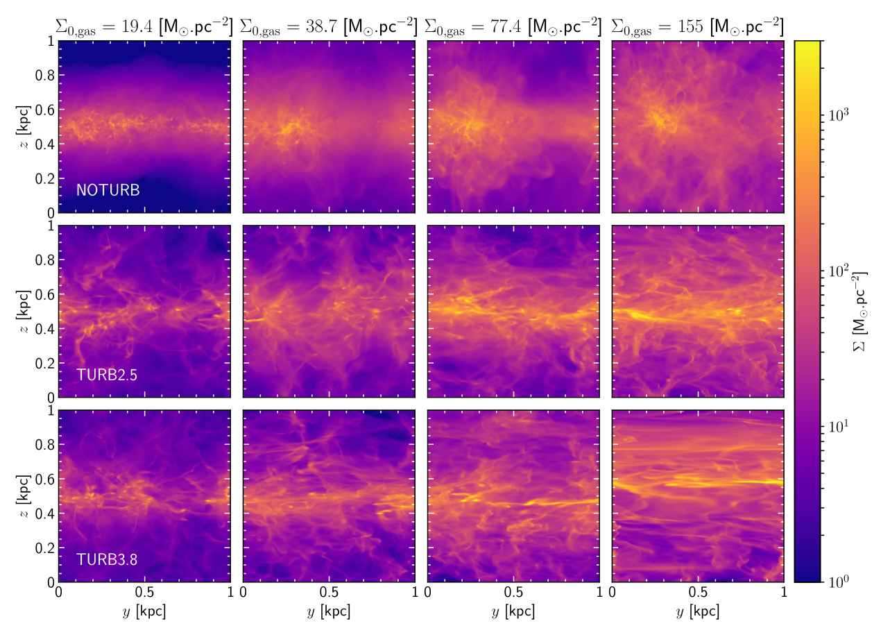
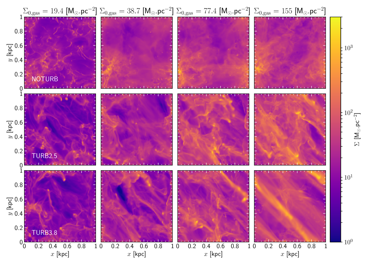
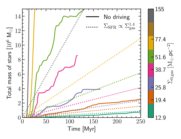
In this section we study the SFR when only stellar feedback regulates star formation (without additional turbulent driving, group noturb). Figure 1 features edge-on and face-on column density maps of the simulations. In noturb simulations, the gas tends to form clumpy structures. Ejection of gas out of the disk plane due to supernovae explosions is clearly visible in the simulations with a high initial gas column density. Figure 2 shows the evolution of the total sink mass during the simulation for several initial column density going from to . The dotted lines correspond to the expected stellar mass growth if the SFR was constant and scaled as in the SK law. For (corresponding to a galaxy slightly heavier than the Milky way) the SFR is close to the observed one for similar galaxies. However, the stellar mass growth is considerably faster than expected in heavier galaxies, with SFR that can overpass the observation by more than one order of magnitude. Interestingly, the SFR also follows a star formation law (see Figure 3a), but with an index , which is much steeper than the determined by Kennicutt. This is unlikely to be due to an underestimation of the stellar feedback. First, all the main processes that may quench the star formation are included in the simulation, except stellar winds. Similar simulations with stellar winds shows that their effect on star formation are not completely negligible but modify it only by a factor of two (Gatto et al., 2017), and thus cannot explain the discrepancies we observe. Second, our FUV prescription (uniform heating proportional to the SFR) overestimates the heating because both absorption and the propagation delay are not well taken into account. Third, additional feedback effects strong enough to reduce star formation to the expected level for would probably generate a too weak SFR for simulations with which are already close to the observed SFR. Finally, Figure 3b shows that the expected turbulent power from stellar feedback is well below what is needed to quench star formation efficiently for high-redshift galaxies. The inefficiency of stellar feedback to quench star formation in gas-rich galaxies suggests that another phenomenon is likely at play.
4 Effects of turbulence injection
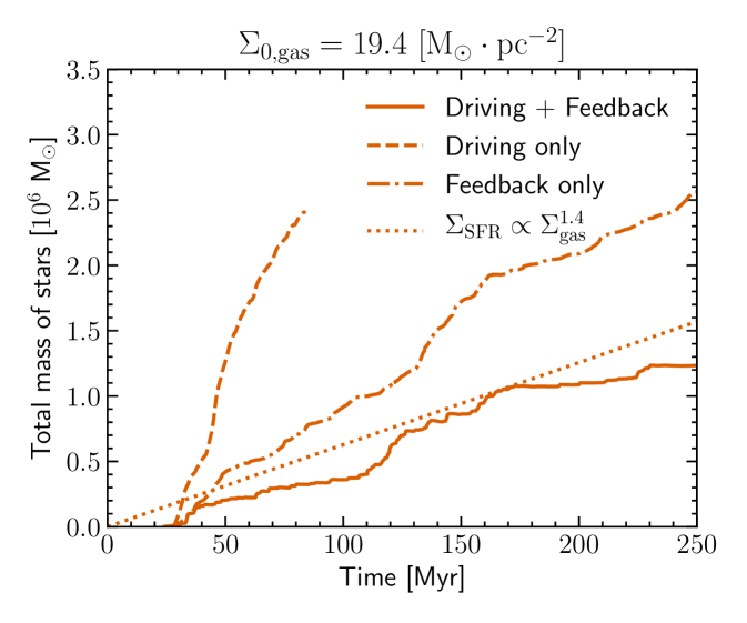
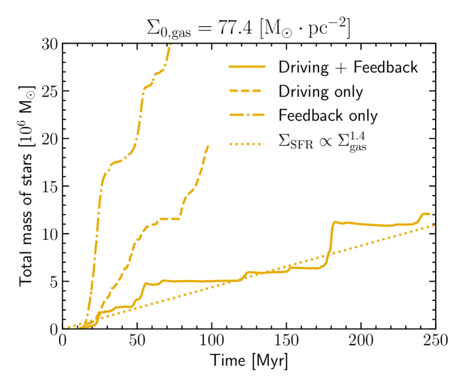
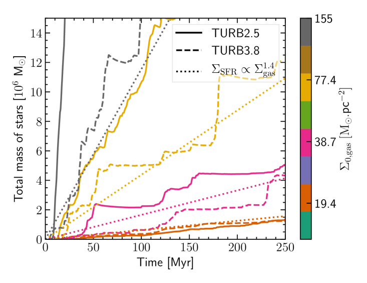
In the previous section we have shown that a pure stellar feedback was not strong enough to quench star formation efficiently in galaxies with high column density. Figure 2 features the mass accreted by the sinks for several values of the initial gas column density with a turbulent forcing (with dominant solenoidal modes). We tested two scalings for the injected energy, and . In both sets of simulations, the stellar mass has been reduced from the pure feedback model, and more powerful driving is more efficient at reducing star formation. The turb3.8 group has stellar mass curve compatible with a SFR matching the SK law.
Indeed, in Figure 3a the star formation law derived from this group has an index , very close to the of the SK relation. Therefore, large-scale turbulent driving enables to reproduce a formation law close to the SK law when pure stellar feedback cannot.
Turbulent driving has a considerable influence on the shape of the galactic disk, as can be seen in Figure 1 representing the face-on and edge-on column density map of gas with and without turbulent driving. Pure feedback simulations show a lot of small-scale structures and clumps, and a lot of gas is blasted out of the disk plane by SNe. When turbulent driving is applied, the gas tends to organize within huge filaments, with fewer and bigger clumps. A significant bulk motion is triggered. The effects of turbulent driving are also clearly visible on the density probability distribution function (PDF) and on the density profile in Figure 6, in the Appendix. When applied, turbulent driving increases the fraction of gas within low-density regions and can move the position of the disk plane. In all cases the scale height of the disk increases for higher value of the column density as the strength of stellar feedback or turbulent driving also increase, but a disk structure is still clearly apparent. More energetic turbulent driving (or 3D turbulent driving) completely destroys the disks, which sets a limit on the turbulent energy that can be injected.
5 Is Stellar Feedback Needed at All?
Previous studies (Bournaud et al., 2010; Renaud et al., 2012; Krumholz et al., 2018; Hopkins et al., 2011) suggest that both large-scale turbulence and stellar feedback are needed to match observations. Block et al. (2010) argue that stellar feedback is crucial to inject energy back to large scales. With our setup, we can carry out a simple experiment to see if stellar feedback is necessary to quench star formation. To investigate this, we rerun two simulations of the turb3.8 group, namely those with and , with stellar feedback off (we switch off H II regions and SNe, and FUV heating is kept constant at solar neighborhood level), so that only the turbulent driving quenches star formation. On Figure 4, we can see that in such a configuration the SFR is higher than the one given by the Kennicutt law. For low gas column density, it is even higher than the one that we obtain with stellar feedback only. Thus, it appears that stellar feedback and large-scale turbulence are complementary to quench star formation, and that the relative importance of stellar feedback diminishes as the gas column density increase. This result is in good agreement with the conclusion reached from global galactic simulations (Bournaud et al., 2010).
6 Conclusion
We have presented simulations of kiloparsec cube regions of galaxies with and without stellar feedback and with and without turbulent driving (Table 1, figures 1,4). The simulated galaxies have a gas column density between and . We reported the SFR in these simulations as function of the gas column density (Figure 2) and compared the obtained star formation law with the SK law (Figure 3a). Then we compared the power injected by the turbulent driving needed to reproduce the SK law with estimates of the turbulent power released by large-scale motions and stellar feedback (Figure 3b). Our main findings are as follows.
-
1.
Stellar feedback is able to explain the SFR in Milky Way–like galaxies.
-
2.
In high-redshift galaxies with high gas column densities, stellar feedback alone is too weak to quench star formation to a level consistent with the SK law: the obtained star formation law for the studied range of gas column densities is too steep compared to the SK law.
-
3.
The addition of a mainly solenoidal large-scale turbulent driving with a power injection reduces considerably the SFR. The star formation obtained has an index , which is close to the observed SK relation.
-
4.
The injected power is consistent with the power needed to maintain the disk at marginal stability (with a Toomre , which scales as .
- 5.
-
6.
Stellar feedback remains necessary, but its importance decreases as the gas column density increases.
Large-scale turbulent driving is therefore necessary when studying star formation in kpc-sized regions of galaxies, especially when the gas fraction is high. A key question that arises is what is the exact nature and origin of the turbulence that needs to be injected.
Appendix A Power injected by the turbulent driving and by the feedback
The section 2.4 provides an estimation on how the power injected via turbulence scales with column density. We can go further and estimate what is the absolute value of power injected, and compare it to the value used for the turb3.8 group of simulation that best reproduce the SK law and to the power injected by stellar feedback (Figure 3b). To get a relevant value, we must take into account the stellar contribution to the Toomre stability criterion. The formula for the Toomre parameter when both the gas and the star fluid are near instability is rather complicated, but the following equation is a acceptable approximation (Wang & Silk, 1994; Romeo & Wiegert, 2011; Romeo & Falstad, 2013)
| (A1) |
with
| (A2) |
The stability criterion is still . For high-redshift galaxies, (Daddi et al., 2010; Genzel et al., 2010) and (as reported by Elmegreen & Elmegreen (2006) with measurement based on the thickness of edge-on stellar disks). In Milky Way–like galaxies, (de Blok et al., 2008) and (Falcón-Barroso et al., 2017; Hennebelle & Falgarone, 2012, and references therein). In both cases, and then
| (A3) |
Using equations 6 and A2 we get
| (A4) |
where we take as typical injection scale (see section 2.3), with the length of one side the box. We take solar neighborhood value for the epicyclic frequency :
| (A5) |
with and . As a result,
| (A6) |
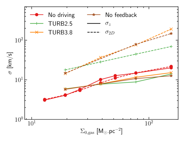
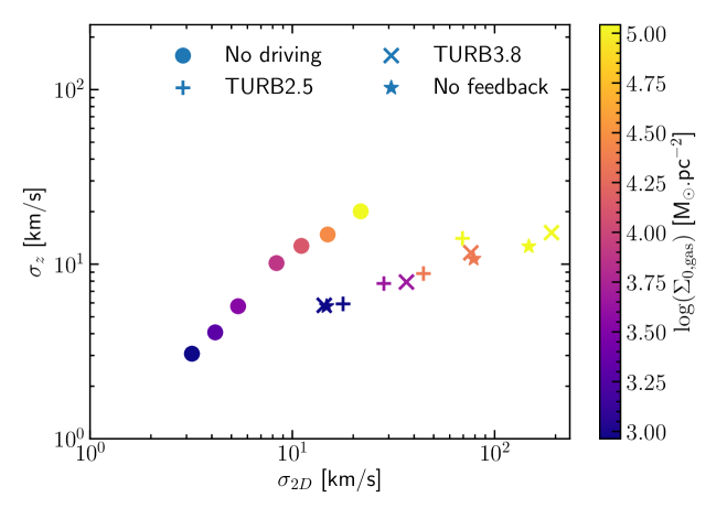
This value is probably a lower bound because the values of the velocity dispersion reported in the observations are usually derived under the assumption of isotropy. However, the velocity dispersion at the scales that we look at is dominated by the 2D velocity dispersion within the disk (Figure 5).
Figure 3b emphasizes another important fact: it is completely unlikely that our turbulent driving mimick the effect of stellar feedback-driven turbulence. Indeed, the energy injected under the form of turbulence by the stellar feedback scales as the SFR, that is , which is not compatible with the relation needed to reproduce the SK law. On Figure 3b, we illustrate this with an estimation of the energy injected by the dominant feedback mechanism, SNe. There is approximately one SN each time of stellar mass is created. It releases erg into the interstellar medium. Iffrig & Hennebelle (2015) and Martizzi et al. (2016) have shown that at these scales, only a fraction of a few percent of this energy is converted into turbulence. We retain values between and as reasonable (red shaded region in Figure 3b). The turbulent power injected by the SN is then
| (A7) |
It is clearly not sufficient for high-redshift galaxies, but dominates over the power as estimated in Equation A4 for Milky way–like galaxies. This is coherent with our result that stellar feedback alone is sufficient in such galaxies.
Appendix B Effect of turbulence on density distribution
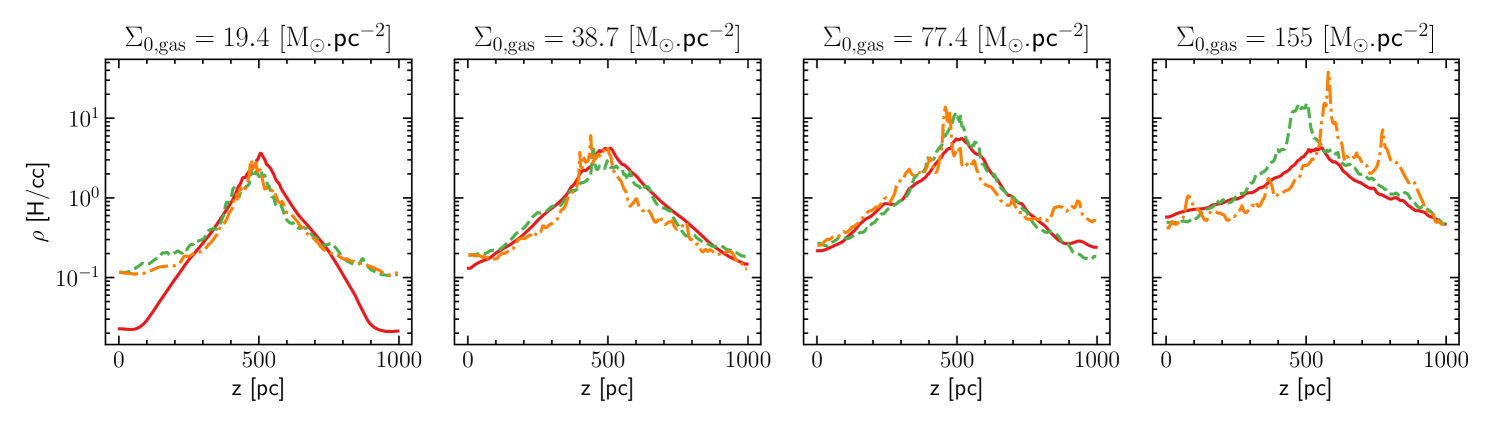
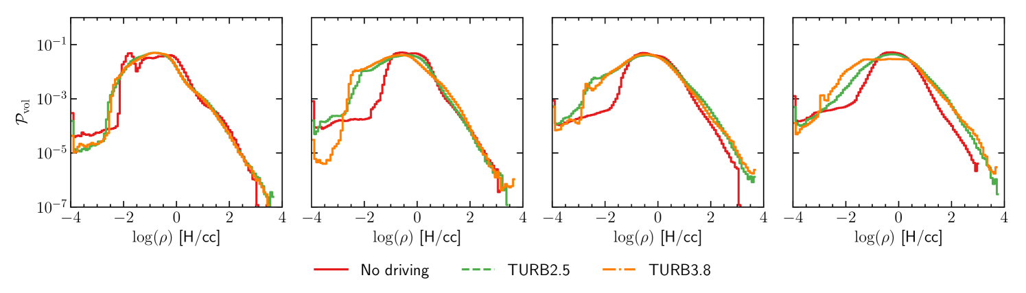
The Figure 6 gives more insight on the effects of the turbulence on the density distribution. The density profile shows that all simulations feature a stratified gas distribution, and that the profile is less steep when the gas column density or the turbulence forcing increase. Strong turbulence (for ) can trigger huge bulk motion that can move the position of the disk plane. Stronger turbulence can even disrupt the disk. The turbulent driving redistributes the gas and widens the gas PDF, increasing the fraction of gas in low-density regions, diminishing the gas available for star formation.
References
- Bleuler & Teyssier (2014) Bleuler, A., & Teyssier, R. 2014, Monthly Notices of the Royal Astronomical Society, 445, 4015. http://adsabs.harvard.edu/abs/2014MNRAS.445.4015B
- Block et al. (2010) Block, D. L., Puerari, I., Elmegreen, B. G., & Bournaud, F. 2010, The Astrophysical Journal Letters, 718, L1. http://adsabs.harvard.edu/abs/2010ApJ...718L...1B
- Bournaud (2014) Bournaud, F. 2014, ASP Conference Series, 486, 101. http://adsabs.harvard.edu/abs/2014ASPC..486..101B
- Bournaud et al. (2010) Bournaud, F., Elmegreen, B. G., Teyssier, R., Block, D. L., & Puerari, I. 2010, <pre>MNRAS</pre>, 409, 1088. http://dx.doi.org/10.1111/j.1365-2966.2010.17370.x
- Colling et al. (2018) Colling, C., Hennebelle, P., Geen, S., Iffrig, O., & Bournaud, F. 2018, A&A, 620, A21
- Daddi et al. (2010) Daddi, E., Bournaud, F., Walter, F., et al. 2010, The Astrophysical Journal, 713, 686. http://adsabs.harvard.edu/abs/2010ApJ...713..686D
- de Blok et al. (2008) de Blok, W. J. G., Walter, F., Brinks, E., et al. 2008, The Astronomical Journal, 136, 2648. http://adsabs.harvard.edu/abs/2008AJ....136.2648D
- Dekel et al. (2009) Dekel, A., Sari, R., & Ceverino, D. 2009, The Astrophysical Journal, 703, 785. http://adsabs.harvard.edu/abs/2009ApJ...703..785D
- Dubois & Teyssier (2008) Dubois, Y., & Teyssier, R. 2008, Astronomy and Astrophysics, 477, 79. http://adsabs.harvard.edu/abs/2008A%26A...477...79D
- Elmegreen & Elmegreen (2006) Elmegreen, B. G., & Elmegreen, D. M. 2006, The Astrophysical Journal, 650, 644. http://adsabs.harvard.edu/abs/2006ApJ...650..644E
- Emsellem et al. (2015) Emsellem, E., Renaud, F., Bournaud, F., et al. 2015, Monthly Notices of the Royal Astronomical Society, 446, 2468. http://adsabs.harvard.edu/abs/2015MNRAS.446.2468E
- Eswaran & Pope (1988) Eswaran, V., & Pope, S. B. 1988, Computers and Fluids, 16, 257
- Falcón-Barroso et al. (2017) Falcón-Barroso, J., Lyubenova, M., van de Ven, G., et al. 2017, Astronomy & Astrophysics, 597, A48. https://www.aanda.org/articles/aa/abs/2017/01/aa28625-16/aa28625-16.html
- Federrath et al. (2010) Federrath, C., Roman-Duval, J., Klessen, R. S., Schmidt, W., & Mac Low, M. M. 2010, A&A, 512, A81. https://ui.adsabs.harvard.edu/abs/2010A&A...512A..81F
- Fromang et al. (2006) Fromang, S., Hennebelle, P., & Teyssier, R. 2006, A&A, 457, 371. http://dx.doi.org/10.1051/0004-6361:20065371
- Gatto et al. (2017) Gatto, A., Walch, S., Naab, T., et al. 2017, Monthly Notices of the Royal Astronomical Society, 466, 1903. http://adsabs.harvard.edu/abs/2017MNRAS.466.1903G
- Genzel et al. (2008) Genzel, R., Burkert, A., Bouché, N., et al. 2008, ApJ, 687, 59
- Genzel et al. (2010) Genzel, R., Tacconi, L. J., Gracia-Carpio, J., et al. 2010, Monthly Notices of the Royal Astronomical Society, 407, 2091. http://adsabs.harvard.edu/abs/2010MNRAS.407.2091G
- Hennebelle & Falgarone (2012) Hennebelle, P., & Falgarone, E. 2012, Astronomy and Astrophysics Review, 20, 55. http://adsabs.harvard.edu/abs/2012A%26ARv..20...55H
- Hopkins et al. (2011) Hopkins, P. F., Quataert, E., & Murray, N. 2011, Monthly Notices of the Royal Astronomical Society, 417, 950. http://adsabs.harvard.edu/abs/2011MNRAS.417..950H
- Iffrig & Hennebelle (2015) Iffrig, O., & Hennebelle, P. 2015, Astronomy and Astrophysics, 576, A95. http://adsabs.harvard.edu/abs/2015A%26A...576A..95I
- Iffrig & Hennebelle (2017) —. 2017, A&A, 604, A70
- Jin et al. (2017) Jin, K., Salim, D. M., Federrath, C., et al. 2017, Monthly Notices of the Royal Astronomical Society, 469, 383. http://adsabs.harvard.edu/abs/2017MNRAS.469..383J
- Kennicutt & Evans (2012) Kennicutt, R. C., & Evans, N. J. 2012, Annual Review of Astronomy and Astrophysics, 50, 531. http://adsabs.harvard.edu/abs/2012ARA%26A..50..531K
- Kennicutt (1998) Kennicutt, Jr., R. C. 1998, ApJ, 498, 541. http://dx.doi.org/10.1086/305588
- Kim & Ostriker (2017) Kim, C.-G., & Ostriker, E. C. 2017, The Astrophysical Journal, 846, 133. http://adsabs.harvard.edu/abs/2017ApJ...846..133K
- Kolmogorov (1941) Kolmogorov, A. 1941, Akademiia Nauk SSSR Doklady, 30, 301
- Krumholz & Burkhart (2016) Krumholz, M. R., & Burkhart, B. 2016, Monthly Notices of the Royal Astronomical Society, 458, 1671. http://adsabs.harvard.edu/abs/2016MNRAS.458.1671K
- Krumholz et al. (2018) Krumholz, M. R., Burkhart, B., Forbes, J. C., & Crocker, R. M. 2018, Monthly Notices of the Royal Astronomical Society, 477, 2716. https://academic.oup.com/mnras/article/477/2/2716/4962399
- Martizzi et al. (2016) Martizzi, D., Fielding, D., Faucher-Giguère, C.-A., & Quataert, E. 2016, Monthly Notices of the Royal Astronomical Society, 459, 2311. http://adsabs.harvard.edu/abs/2016MNRAS.459.2311M
- Meidt et al. (2020) Meidt, S. E., Glover, S. C. O., Kruijssen, J. M. D., et al. 2020, ApJ, 892, 73
- Ostriker et al. (2010) Ostriker, E. C., McKee, C. F., & Leroy, A. K. 2010, ApJ, 721, 975
- Padoan et al. (2016) Padoan, P., Pan, L., Haugbølle, T., & Nordlund, Å. 2016, The Astrophysical Journal, 822, 11. http://adsabs.harvard.edu/abs/2016ApJ...822...11P
- Renaud et al. (2012) Renaud, F., Kraljic, K., & Bournaud, F. 2012, The Astrophysical Journal Letters, 760, L16. http://adsabs.harvard.edu/abs/2012ApJ...760L..16R
- Romeo & Falstad (2013) Romeo, A. B., & Falstad, N. 2013, Monthly Notices of the Royal Astronomical Society, 433, 1389. http://adsabs.harvard.edu/abs/2013MNRAS.433.1389R
- Romeo & Wiegert (2011) Romeo, A. B., & Wiegert, J. 2011, Monthly Notices of the Royal Astronomical Society, 416, 1191. http://adsabs.harvard.edu/abs/2011MNRAS.416.1191R
- Schmidt et al. (2009) Schmidt, W., Federrath, C., Hupp, M., Kern, S., & Niemeyer, J. C. 2009, A&A, 494, 127. http://dx.doi.org/10.1051/0004-6361:200809967
- Schmidt et al. (2006) Schmidt, W., Hillebrandt, W., & Niemeyer, J. C. 2006, Computers & Fluids, 35, 353. http://www.sciencedirect.com/science/article/pii/S0045793005000563
- Teyssier (2002) Teyssier, R. 2002, Astronomy and Astrophysics, 385, 337. https://ui.adsabs.harvard.edu/abs/2002A&A...385..337T
- Walch et al. (2015) Walch, S., Girichidis, P., Naab, T., et al. 2015, Monthly Notices of the Royal Astronomical Society, 454, 238. http://adsabs.harvard.edu/abs/2015MNRAS.454..238W
- Wang & Silk (1994) Wang, B., & Silk, J. 1994, The Astrophysical Journal, 427, 759. http://adsabs.harvard.edu/abs/1994ApJ...427..759W