This paper was converted on www.awesomepapers.org from LaTeX by an anonymous user.
Want to know more? Visit the Converter page.

Large subgraphs in pseudo-random graphs

Anirban Basak Shankar Bhamidi Suman Chakraborty  and  Andrew Nobel§ Department of Mathematics, Weizmann Institute of Science,
POB 26, Rehovot 76100, Israel
†‡§Department of Statistics & Operations Research,
University of North Carolina at Chapel Hill,
318 Hanes Hall, CB# 3260, Chapel Hill, NC 27599, USA
(Date: September 6, 2025)
Abstract.

We consider classes of pseudo-random graphs on nn vertices for which the degree of every vertex and the co-degree between every pair of vertices are in the intervals (npCnδ,np+Cnδ)(np-Cn^{\delta},np+Cn^{\delta}) and (np2Cnδ,np2+Cnδ)(np^{2}-Cn^{\delta},np^{2}+Cn^{\delta}) respectively, for some absolute constant CC, and p,δ(0,1)p,\delta\in(0,1). We show that for such pseudo-random graphs the number of induced isomorphic copies of subgraphs of size ss are approximately same as that of an Erdős-Réyni random graph with edge connectivity probability pp as long as s(((1δ)12)o(1))logn/log(1/p)s\leq(((1-\delta)\wedge\frac{1}{2})-o(1))\log n/\log(1/p), when p(0,1/2]p\in(0,1/2]. When p(1/2,1)p\in(1/2,1) we obtain a similar result. Our result is applicable for a large class of random and deterministic graphs including exponential random graph models (ERGMs), thresholded graphs from high-dimensional correlation networks, Erdős-Réyni random graphs conditioned on large cliques, random dd-regular graphs and graphs obtained from vector spaces over binary fields. In the context of the last example, the results obtained are optimal. Straight-forward extensions using the proof techniques in this paper imply strengthening of the above results in the context of larger motifs if a model allows control over higher co-degree type functionals.

1. Introduction

In the context of probabilistic combinatorics, the origin of random graphs dates back to [29] where Erdős used probabilistic methods to show the existence of a graph with certain Ramsey property. Soon after some of the foundational work on random graphs was established in [25, 26, 27]. The simplest model of random graph is as follows: Fix n1n\geq 1 and start with vertex set {1,2,,n}\{1,2,\ldots,n\}. For ease of notation hereafter, we denote [n]:={1,2,,n}[n]:=\{1,2,\ldots,n\}. Fix p(0,1)p\in(0,1). The graph is formed by randomly drawing an edge between every pair of vertices ij[n]i\neq j\in[n], with probability pp. This random graph is known as Erdős-Réyni random graph with edge connectivity probability pp. In the sequel we use 𝖦(n,p){\sf G}(n,p) to denote this graph (also known as binomial random graph in the literature). This model has stimulated an enormous amount of work over the last fifty years aimed at understanding properties of 𝖦(n,p){\sf G}(n,p) (see [6, 31] and the references therein) in particular in the large network nn\to\infty limit.

In the last decade there has been an explosion in the amount of empirical data on real world networks in a wide array of fields including statistics, machine learning, computer science, sociology, epidemiology. This has stimulated the development of a multitude of models to explain many of the properties of real world networks including high clustering coefficient, heavy tailed degree distribution and small world properties; see e.g. [34, 1] for wide-ranging surveys; see [23, 41, 17] for a survey of rigorous results on the formulated models. Although such network models are not as simple as an Erdős-Rényi graph, one would still like to investigate whether these posses properties similar to an Erdős-Rényi graph. Therefore, it is natural to ask about how similar/dissimilar such network models are compared to an Erdős-Rényi graph. Many researchers have delved deep into these questions and have found various conditions under which a given graph 𝖦n:=([n],En){\sf G}_{n}:=([n],E_{n}), with vertex set [n][n] and edge set EnE_{n} looks similar to an Erdős-Rényi random graph. In literature these graphs are known by various names. Following Krivelevich and Sudakov [32], we call them pseudo-random graphs.

One key property of an Erdős-Rényi random graph is the following: For any two subsets of vertices U,W[n]U,W\subset[n] the number of edges in a 𝖦(n,p){\sf G}(n,p), whose one end point is in UU and the other is in WW, is roughly equal to p|U||W|p|U||W|, where |||\cdot| denotes the cardinality of a set. Hence, if a pseudo-random graph 𝖦n{\sf G}_{n} is similar to 𝖦(n,p){\sf G}(n,p), then it must also satisfy similar properties. This motivated researchers to consider graphs which possess the above property.

Foundational work for these sorts of questions began with Thomason [37, 38] in the mid-eighties where he used the term Jumbled graph (see Definition 3.1) to describe such graphs. Roughly it provided quantitative bounds on similarity between pseudo-random graphs and a 𝖦(n,p){\sf G}(n,p). This study provided some examples of jumbled graphs and explored various properties of them. It exposed a whole new interesting research area and numerous results were obtained afterwards. Further fundamental work in this area was established by Chung, Graham, and Wilson in [16]. They coined the term quasi-random graphs to describe their models of pseudo-random graphs. They provided several equivalent conditions of pseudo-randomness; one of their major results is described in Section 3, Theorem 3.2 . Paraphrasing these results, loosely they state the following:

For a graph 𝖦n{\sf G}_{n} to be pseudo-random one must have that the number of induced isomorphic copies of any subgraph 𝖧{\sf H} of fixed size (e.g. 𝖧{\sf H} is a triangle) must be roughly equal to that of a 𝖦(n,p){\sf G}(n,p).

Another class of pseudo-random graphs is Alon’s (n,d,λ)(n,d,\lambda)-graph (see [2]). These graphs are dd-regular graphs on nn vertices such that the second largest absolute eigenvalue of its adjacency matrix is less than or equal to λ\lambda. Various graph properties are known for (n,d,λ)(n,d,\lambda)-graphs (see [32] and the references therein).

As described above, the availability of data on real-world networks has stimulated a host of questions in an array of field, in particular in finding large motifs in observed networks such as large cliques or communities (representing interesting patterns in biological or social networks) or understanding the limits of search algorithms in cryptology. Many of these questions are computationally hard and one is left with brute search algorithms over all possible subgraphs of a fixed size to check existence of such motifs. Thus a natural question (again loosely stated) is as follows:

Can we find simple conditions on a sequence of graphs {𝖦n:n1}\{{\sf G}_{n}:n\geqslant 1\} such that the number of induced isomorphic copies of any subgraph 𝖧{\sf H} of growing size (e.g. 𝖧{\sf H} is a clique of size logn\log{n}) must be roughly equal to that in 𝖦(n,p){\sf G}(n,p)? What are the fundamental limits of such conditions?

Here we consider a class of pesudo-random graphs and study the number of induced copies of large subgraphs in those. More precisely, we will assume that our graph 𝖦n{\sf G}_{n} satisfies the following two assumptions for some absolute constant CC, and p,δ(0,1)p,\delta\in(0,1):

Assumption A1.

maxv[n]||𝒩v|np|<Cnδ.\max_{v\in[n]}{\left|\left|\mathscr{N}_{v}\right|-{n}p\right|}<Cn^{\delta}.

Assumption A2.

maxvv[n]||𝒩v𝒩v|np2|<Cnδ.\max_{v\neq v^{\prime}\in[n]}{\left|\left|\mathscr{N}_{v}\cap\mathscr{N}_{v^{\prime}}\right|-{n}p^{2}\right|}<Cn^{\delta}.

Here for any v[n]v\in[n], 𝒩v:={u[n]:uv}\mathscr{N}_{v}:=\{u\in[n]:u\sim v\}, where uvu\sim v means that uu is connected to vv by an edge in 𝖦n{\sf G}_{n}. These two conditions are very natural to assume. For example, using Hoeffding’s ineqaulity it is easy to check that for 𝖦(n,p){\sf G}(n,p) assumptions (A1) and (A2) are satisfied for any δ>1/2\delta>1/2 with super-polynomially high probability. As we will see below, besides 𝖦(n,p){\sf G}(n,p) there are many examples of graph ensembles which satisfy assumptions (A1)-(A2). Further, these two specifications are quite basic and often very easy to check for a given graph (random or deterministic).

In our main theorem below we show that for any such graph sequence the number of induced isomorphic copies of any slowly growing sub-graph is approximately same as that of an Erdős-Rényi random graph with edge connectivity pp. Before stating our main theorem let us introduce some notation: For any rr\in\mathbb{N}, let us denote 𝒢(r)\mathcal{G}(r) be the collection of all graph with vertex set [r][r]. Further given any graph 𝖧{\sf H}, denote n𝖦n(𝖧)n_{{\sf G}_{n}}({\sf H}) to be the number of induced isomorphic copies of 𝖧{\sf H} in 𝖦n{\sf G}_{n} and E(𝖧)E({\sf H}) to be edge-set of 𝖧{\sf H}. Next, for p(0,1)p\in(0,1), define γp:=max{p1,(1p)1}\gamma_{p}:=\max\{p^{-1},(1-p)^{-1}\}. We also write log()\log(\cdot) to denote the natural logarithm, i.e. logarithm with respect to the base ee. When needed, we will specify the base bb and write as logb()\log_{b}(\cdot). For any two positive integers sns\leq n, let us denote (n)s:=n(n1)(ns+1)(n)_{s}:=n(n-1)\cdots(n-s+1). Now we are ready to state our main theorem.

Theorem 1.1.

Let {𝖦n}n\{{\sf G}_{n}\}_{n\in\mathbb{N}} be a sequence of graphs satisfying assumptions (A1) and (A2). Then, there exists a positive constant C0C_{0}^{\prime}, depending on pp, such that

maxs((1δ)12)lognlogγpC0loglognmax𝖧s𝒢(s)|n𝖦n(𝖧s)(n)s|Aut(𝖧s)|(p1p)|E(𝖧s)|(1p)(s2)1|0,\max_{s\leq((1-\delta)\wedge\frac{1}{2})\frac{\log n}{\log\gamma_{p}}-C_{0}^{\prime}\log\log n}\max_{{\sf H}_{s}\in\mathcal{G}(s)}\left|\frac{n_{{\sf G}_{n}}({\sf H}_{s})}{\frac{(n)_{s}}{|\mathrm{Aut}({\sf H}_{s})|}\left(\frac{p}{1-p}\right)^{|E({\sf H}_{s})|}(1-p)^{{s\choose 2}}}-1\right|\rightarrow 0, (1.1)

as nn\rightarrow\infty.


Remark 1.2.

Note that

𝔼(n𝖦(n,p)(𝖧s))=(n)s|Aut(𝖧)|(p1p)|E(𝖧)|(1p)(s2).\mathbb{E}(n_{{\sf G}(n,p)}({\sf H}_{s}))=\frac{(n)_{s}}{|\mathrm{Aut}({\sf H})|}\left(\frac{p}{1-p}\right)^{|E({\sf H})|}(1-p)^{{s\choose 2}}.

Thus Theorem 1.1 establishes that the number of induced isomorphic copies of large graphs are approximately same as that of an Erdős-Rényi graph. In the proof of Theorem 1.1 we actually obtain bounds on the rate of convergence to zero of the lhs of (1.1). Using these rates, one can allow min{p,1p}\min\{p,1-p\} and 1δ1-\delta to go to zero and obtain modified versions of (1.1) in those cases. See Remark 7.8 for more details. For clarity of presentation we work with fixed values of pp and δ\delta in Theorem 1.1. In Section 2.5 we give an example of a graph model where the result Theorem 1.1 is optimal.

Remark 1.3 (Existence of large motifs).

The above result shows that under assumptions (A1) and (A2), the associated sequences of graphs are strongly pseudo-regular in the sense that the count of large motifs in the graph is approximately the same as in Erdős-Rényi random graph. A weaker question is asking existence of large motifs; to fix ideas let r=clognr=c\log{n} for a constant c>0c>0 and 𝖢r{\sf C}_{r} denote a clique on rr vertices. Then one could ask the import of Assumptions (A1) and (A2) on the existence of 𝖢r{\sf C}_{r}; this corresponds to

lim infnn𝖦n(𝖢r)>0.\liminf_{n\to\infty}n_{{\sf G}_{n}}({\sf C}_{r})>0.

We study these questions in work in progress.

We will see in Section 2.5 that the conclusion of Theorem 1.1 cannot be improved unless one has more assumptions on the graph sequence. Below we consider one such direction to understand the implications of our proof technique if one were to assume bounds on the number of common neighbors of three and four vertices.

Assumption A3.

maxv1v2v3[n]||𝒩v1𝒩v3𝒩v3|np3|<Cnδ.\max_{v_{1}\neq v_{2}\neq v_{3}\in[n]}{\left|\left|\mathscr{N}_{v_{1}}\cap\mathscr{N}_{v_{3}}\cap\mathscr{N}_{v_{3}}\right|-{n}p^{3}\right|}<Cn^{\delta}.

Assumption A4.

maxv1v2v3v4[n]||𝒩v1𝒩v3𝒩v3𝒩v4|np4|<Cnδ.\max_{v_{1}\neq v_{2}\neq v_{3}\neq v_{4}\in[n]}{\left|\left|\mathscr{N}_{v_{1}}\cap\mathscr{N}_{v_{3}}\cap\mathscr{N}_{v_{3}}\cap\mathscr{N}_{v_{4}}\right|-{n}p^{4}\right|}<Cn^{\delta}.

Under these above two assumptions we obtain the following improvement of Theorem 1.1.

Theorem 1.4.

Let {𝖦n}n\{{\sf G}_{n}\}_{n\in\mathbb{N}} be a sequence of graphs satisfying assumptions (A1)-(A4). Then, there exists a positive constant C5C_{5}^{\prime}, depending on pp, such that

maxs((1δ)23)lognlogγpC5loglognmax𝖧s𝒢(s)|n𝖦n(𝖧s)(n)s|Aut(𝖧)|(p1p)|E(𝖧)|(1p)(s2)1|0,\max_{s\leq((1-\delta)\wedge\frac{2}{3})\frac{\log n}{\log\gamma_{p}}-C_{5}^{\prime}\log\log n}\max_{{\sf H}_{s}\in\mathcal{G}(s)}\left|\frac{n_{{\sf G}_{n}}({\sf H}_{s})}{\frac{(n)_{s}}{|\mathrm{Aut}({\sf H})|}\left(\frac{p}{1-p}\right)^{|E({\sf H})|}(1-p)^{{s\choose 2}}}-1\right|\rightarrow 0, (1.2)

as nn\rightarrow\infty.


From the proof of Theorem 1.4 it will be clear that adding more assumptions on the common neighbors of a larger collection of vertices may further improve Theorem 1.1. To keep the presentation of current work to manageable length we restrict ourselves only to the above extension. Proof of Theorem 1.4 can be found in Section 7.

We defer a full discussion of related work to Section 3. The rest of this paper is organized as follows:

Outline of the paper.

  1. (i)

    In Section 2 we apply Theorem 1.1 to exponential random graph models (ergms) in the high temperature regime (Section 2.1), random geometric graphs (Section 2.2), conditioned Erdős-Rényi random graphs (Section 2.3), and random regular graphs (Section 2.4). Section 2.5 describes a network model where Theorem 1.1 is optimal. Proofs of all these results can be found in Section 8.

  2. (ii)

    Section 3 discusses the relevance of our results, connections to existing literature as well as possible extensions and future directions to pursue.

  3. (iii)

    In Section 4 we provide an outline of our proof technique. We start this section by stating Proposition 4.1, which is the sub-case of Theorem 1.1 for p=1/2p=1/2. For clarity of presentation, we only explain the idea behind the proof of Proposition 4.1. Along with the proof idea we introduce necessary notation and definitions.

  4. (iv)

    We prove Proposition 4.1 in Section 5. We state the lemmas needed to prove Proposition 4.1. Proofs of these lemmas are deferred to Section 6.

  5. (v)

    In Section 7 we provide a detailed outline about how one can extend the ideas from the proof of Proposition 4.1 to prove Theorem 1.1. Proof of Theorem 1.4 can also be found in Section 7. Section 8 contains proofs for the applications our main result.

2. Applications of Theorem 1.1

In this section we consider four different random graph ensembles: exponential random graph models, random geometric graphs, Erdős-Rényi random graphs conditioned on a large clique, and random dd-regular graphs. We show that for these four random graph ensembles Theorem 1.1 can be applied (and adapted) to show that the number of induced isomorphic slowly growing subgraphs are close to that of an Erdős-Rényi random graph. In Section 2.5 considering an example of a sequence of deterministic graphs we show that one may not extend the conclusion of Theorem 1.1 without any additional assumptions on the graph sequence.

2.1. Exponential random graph models (ergm)

The exponential random graph model (ergm) is one of the most widely used models in areas such as sociology and political science since it gives a flexible method for capturing reciprocity (or clustering behavior) observed in most real world social networks. The last few years have seen major breakthroughs in rigorously understanding the behavior of ergm in the large network nn\to\infty limt (see [5, 15] and the references therein). It has been shown that in the high temperature regime (which we precisely define in Assumption 2.1), these models converge in the so-called cut-distance, a notion of distance between graphs established in [7], [8], to the same limit as an Erdős-Rényi random graph as the number of vertices increase, where the edge connectivity probability of the Erdős-Rényi random graph is determined explicitly by a function of the parameters (see [15]). In particular this implies that the number of induced isomorphic copies of any subgraph on fixed number of vertices are asymptotically same as in an Erdős-Rényi random graph in that high temperature regime (see [7, Theorem 2.6]). In this section we strengthen the above result to show that in the high temperature regime the number of induced isomorphic copies of subgraphs of growing size in an ergm are approximately same with that of an Erdős-Rényi graph, with appropriate edge connectivity probability.

We start with a precise formulation of the model. We will stick to the simplest specification of this model which incorporates edges and triangles although we believe that the results below carry over for any model in the ferromagnetic case as long as one is in the high temperature regime. Let Ω:={0,1}(n2)\Omega:=\{0,1\}^{{n\choose 2}} and note that any simple graph on nn vertices can be represented by a tuple 𝒙:=(xij)1i<jnΩ\bm{x}:=(x_{ij})_{1\leqslant i<j\leqslant n}\in\Omega. Here xij=1x_{ij}=1 if vertices i,ji,j are connected by an edge and xij=0x_{ij}=0 otherwise. On this space, we define the Hamiltonian HH as follows.

H(𝒙):=β1i<jnxij+γn1i<j<knxijxjkxik.H(\bm{x}):=\beta\sum_{1\leqslant i<j\leqslant n}x_{ij}+\frac{\gamma}{n}\sum_{1\leqslant i<j<k\leqslant n}x_{ij}x_{jk}x_{ik}. (2.1)

Note that E(𝒙):=1i<jnxijE(\bm{x}):=\sum_{1\leqslant i<j\leqslant n}x_{ij} is just the number of edges in 𝒙\bm{x} whilst T(𝒙):=1i<j<knxijxjkxikT(\bm{x}):=\sum_{1\leqslant i<j<k\leqslant n}x_{ij}x_{jk}x_{ik} is the number of triangles. Thus the above Hamiltonian has a simpler interpretation as

H(𝒙)=βE(𝒙)+γnT(𝒙).H(\bm{x})=\beta E(\bm{x})+\frac{\gamma}{n}T(\bm{x}).

For simplicity we write 𝜷:=(β,γ)\bm{\beta}:=(\beta,\gamma) for the parameters of the model, and consider the probability measure,

p𝜷(n)(𝒙)exp(H(𝒙)),𝒙Ω.p_{\bm{\beta}}^{\scriptscriptstyle(n)}(\bm{x})\propto\exp(H(\bm{x})),\qquad\bm{x}\in\Omega. (2.2)

In the sequel, to ease notation, we will suppress nn and write the above, often as p𝜷p_{\bm{\beta}}. Now for later use we define the function φ𝜷:[0,1][0,1]\varphi_{\bm{\beta}}:[0,1]\to[0,1] via,

φ𝜷(x):=eβ+γx1+eβ+γx.\varphi_{\bm{\beta}}(x):=\frac{e^{\beta+\gamma x}}{1+e^{\beta+\gamma x}}. (2.3)

Below we state the assumption on the ergm with which we work in this paper.

Assumption 2.1.

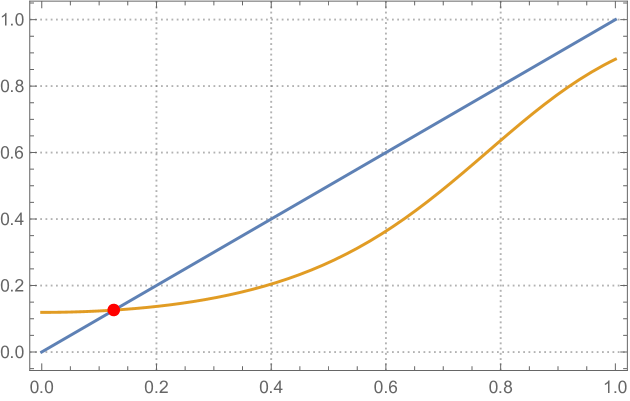
We assume that we are in the ferromagnetic regime, namely γ>0\gamma>0. Further we assume that the parameters 𝜷\bm{\beta} are in the high temperature regime (see also [5]). That is, there exists a unique solution 0<p<10<p^{*}<1 to the equation

p=eβ+γp21+eβ+γp2p=\frac{e^{\beta+\gamma p^{2}}}{1+e^{\beta+\gamma p^{2}}} (2.4)

and further

ddpeβ+γp21+eβ+γp2|p=p<1.\left.\frac{d}{dp}\frac{e^{\beta+\gamma p^{2}}}{1+e^{\beta+\gamma p^{2}}}\right|_{p=p^{*}}<1. (2.5)

See Figure 1 below for a graphical description of our setting. In passing we note that the above two conditions can be succinctly expressed using the function φ𝜷\varphi_{\bm{\beta}} as defined in (2.3) as,

p=φ𝜷((p)2),ddpφ𝜷(p2)|p=p<1.p^{*}=\varphi_{\bm{\beta}}((p^{*})^{2}),\qquad\left.\frac{d}{dp}\varphi_{\bm{\beta}}(p^{2})\right|_{p=p^{*}}<1. (2.6)
Refer to caption
Figure 1. The functions f(p)=pf(p)=p and g(p)=eβ+γp21+eβ+γp2g(p)=\frac{e^{\beta+\gamma p^{2}}}{1+e^{\beta+\gamma p^{2}}} with β=2\beta=-2 and γ=4\gamma=4. The red point corresponds to pp^{*}.

Now we are ready to state the main result regarding ergm.

Theorem 2.2.

Let 𝖦(n,p){\sf G}(n,p^{*}) denote an Erdős-Rényi random graph with edge connectivity probability pp^{*}. Let 𝐗(n)p𝛃(n)\bm{X}^{\scriptscriptstyle(n)}\sim p_{\bm{\beta}}^{\scriptscriptstyle(n)} satisfying assumption 2.1. Then as nn\to\infty, we have,

maxs12lognlogγpC1loglognmax𝖧s𝒢(s)|n𝑿(n)(𝖧s)𝔼(n𝖦(n,p)(𝖧s))  1|0, almost surely,\max_{s\leq\frac{1}{2}\frac{\log n}{\log\gamma_{p^{*}}}-C_{1}^{\prime}\log\log\hskip-2.0ptn}\max_{{\sf H}_{s}\in\mathcal{G}(s)}\left|\frac{n_{\bm{X}^{\scriptscriptstyle(n)}}({\sf H}_{s})}{\mathbb{E}(n_{{\sf G}(n,p^{*})}({\sf H}_{s}))}\;\;-\;\;1\right|\rightarrow 0,\text{ almost surely},

where C1C_{1}^{\prime} is some positive constant depending only on pp^{*}.


Theorem 2.2 follows from Theorem 1.1 once we establish that assumptions (A1)-(A2) are satisfied by 𝑿(n){\bm{X}^{\scriptscriptstyle(n)}} almost surely. We defer the proof to Section 8.

2.2. Thresholded graphs from high-dimensional correlation networks

In this section we consider thresholded graphs obtained from high-dimensional random geometric graphs. Roughly in a geometric graph the vertices are points in some metric space and two vertices are connected if they are within a specified threshold distance. These models have drawn wide interests from different branches of science such as machine learning, statistics etc. It is of interest to study these graphs when the dimension of the underlying metric space is growing with the number of vertices. In the context of applications, one major are of applications of this model is neuroscience, while it is impossible to give even a representative sample of related papers, a starting point would be [11, 35, 24] and the references therein. Paraphrasing from [11, Page 187] (with parts (c) and (d) most relevant for this paper):

“Structural and functional brain networks can be explored using graph theory through the following four steps: ”

  1. (a)

    Define the network nodes. These could be defined as electroencephalography or multielectrode-array electrodes, or as anatomically defined regions of histological, MRI or diffusion tensor imaging data.

  2. (b)

    Estimate a continuous measure of association between nodes. This could be the spectral coherence or Granger causality measures between two magnetoencephalography sensors, \ldots or the inter-regional correlations in cortical thickness or volume MRI measurements estimated in groups of subjects.

  3. (c)

    Generate an association matrix by compiling all pairwise associations between nodes and (usually) apply a threshold to each element of this matrix to produce a binary adjacency matrix or undirected graph.

  4. (d)

    Calculate the network parameters of interest in this graphical model of a brain network and compare them to the equivalent parameters of a population of random networks.”

As a test-bed, we study the simplest possible setting for such questions, first studied rigorously in [21] and [10], and study the behavior of the graph as dimension is growing with the number of vertices. To describe the model, we closely follow [21]. Write 𝒮d1:={𝒙d:𝒙2=1}\mathscr{S}_{d-1}:=\{\bm{x}\in\mathbb{R}^{d}:\|\bm{x}\|_{2}=1\} for the unit sphere in d\mathbb{R}^{d}, where 2\|\cdot\|_{2} denotes the usual Euclidean metric. Suppose {𝑿i:i[n]}\{\bm{X}_{i}:i\in[n]\} be nn points chosen independently and uniformly distributed on 𝒮d1\mathscr{S}_{d-1}. Fix p(0,1)p\in(0,1). We will use these points to construct a graph with vertex set [n][n] as follows: For ij[n]i\neq j\in[n] say that vertex ii is connected to jj if and only if

𝑿i,𝑿jtp,d.\langle\bm{X}_{i},\bm{X}_{j}\rangle\geqslant t_{p,d}.

Here ,\langle\cdot,\cdot\rangle is the usual inner product operation on d\mathbb{R}^{d} and tp,dt_{p,d} is a constant chosen such that

(𝑿i,𝑿jtp,d)=p\mathbb{P}(\langle\bm{X}_{i},\bm{X}_{j}\rangle\geqslant t_{p,d})=p (2.7)

Call the resulting graph 𝖦(n,d,p){\sf G}(n,d,p). See Figure 2 for a pictorial representation.

𝐞𝟏\mathbf{e_{1}}𝐗𝐢\mathbf{X_{i}}θ\theta
Figure 2. A vertex ii is connected 11 in 𝖦(n,d,p){\sf G}(n,d,p) if and only if cos(θ)tp,d\cos(\theta)\geqslant t_{p,d}. Here we have rotated the original points via an orthogonal transformation so that the co-ordinates of vertex 11 correspond to 𝐞𝟏=(1,0,,0)\mathbf{e_{1}}=(1,0,\ldots,0). Picture modified from template on https://github.com/MartinThoma/LaTeX-examples.

Maximal clique behavior in this model was studied in [21]. Further it was shown in [21] that the total variation distance between 𝖦(n,d,p){\sf G}(n,d,p) and 𝖦(n,p){\sf G}(n,p) goes to zero as dd\rightarrow\infty while nn is fixed. It was further shown in [10] that the total variation distance between 𝖦(n,d,p){\sf G}(n,d,p) and 𝖦(n,p){\sf G}(n,p) goes to zero if dd grows faster than n3n^{3} while the distance goes to 11 if d/n30d/n^{3}\rightarrow 0. In this section we will consider weaker notions of convergence of graphs and establish that random geometric graphs look similar to Erdős-Rényi when dd is growing as slow as (logn)c(\log n)^{c} for some c>1c>1. Below we work with following assumption on random geometric graphs.

Assumption 2.3.

We consider random geometric graphs 𝖦(d,n,p){\sf G}(d,n,p) with 0<p1/20<p\leqslant 1/2 and d/lognd/\log{n}\to\infty as nn\rightarrow\infty.

We split our result on 𝖦(d,n,p){\sf G}(d,n,p) into two parts. In first part we consider induced isomorphic copies of any fixed graph.

Theorem 2.4.

If (logn)c/d=o(1)(\log n)^{c}/d=o(1) for some c>1c>1, then as nn\to\infty and we have,

|n𝖦(n,d,p)(𝖧)𝔼(n𝖦(n,p)(𝖧))  1|0, almost surely,\left|\frac{n_{{\sf G}(n,d,p)}({\sf H})}{\mathbb{E}(n_{{\sf G}(n,p)}({\sf H}))}\;\;-\;\;1\right|\rightarrow 0,\text{ almost surely},

for all finite subgraph 𝖧{\sf H}.

Theorem 2.4 shows that the number of induced isomorphic copies of any fixed graph is asymptotically same as that of an Erdős-Rényi random graph. Therefore, from [7, Theorem 2.6] it follows that 𝖦(d,n,p){\sf G}(d,n,p) and 𝖦(n,p){\sf G}(n,p) are arbitrarily close in cut-metric as soon as dd is poly-logarithmic in nn. Theorem 2.4 is actually a consequence of the following stronger result. This result shows that the number of copies of “large subgraphs” are asymptotically same as that of Erdős-Rényi random graph. However, the size of the subgraphs one can consider depends on how fast dd “grows” compared to nn. More precisely, we have the following result.

Theorem 2.5.

Let 𝖦(d,n,p){\sf G}(d,n,p) be a random geometric graph on nn vertices satisfying Assumption 2.3. Then, we have,

maxslogτn1/logγpC2loglogτn1max𝖧s𝒢(s)|n𝖦(n,d,p)(𝖧s)𝔼(n𝖦(n,p)(𝖧s))  1|0, almost surely,\max_{s\leq{\log\tau_{n}^{-1}}/{\log\gamma_{p}}-C_{2}^{\prime}\log\log\tau_{n}^{-1}}\max_{{\sf H}_{s}\in\mathcal{G}(s)}\left|\frac{n_{{\sf G}(n,d,p)}({\sf H}_{s})}{\mathbb{E}(n_{{\sf G}(n,p)}({\sf H}_{s}))}\;\;-\;\;1\right|\rightarrow 0,\text{ almost surely},

where

τn:=κp[max{logn,logd}d+1n2],\tau_{n}:=\kappa_{p}\left[\sqrt{\frac{\max\{\log{n},\log{d}\}}{d}}+\frac{1}{n^{2}}\right],

for some large positive constants κp\kappa_{p} and C2C_{2}^{\prime}.


Remark 2.6.

Note that if dd is poly-logarithmic in nn then from Theorem 2.5 it follows that the number of induced isomorphic copies of subgraphs of size upto O(loglogn)O(\log\log n) are roughly same as that an Erdős-Rényi random graph. Proof of Theorem 2.5 can be found in Section 8. As described in Remark 1.3 the question considered in this paper is refined in the sense that we want the number of large motifs in the model under consideration to closely match the corresponding number in an Erdős-Rényi random graph; this second object grows exponentially in the size of the motif being considered. Thus small errors build up as will be seen in the proofs. In future work we will consider the problem described in Remark 1.3 where one is only interested in the existence of large motifs.

2.3. Erdős-Rényi random graphs conditioned on large cliques

Finding maximal cliques in graphs is a fundamental problem in computational complexity. One natural direction of research is average case analysis; more precisely studying this problem in the context of the Erdős-Rényi random graph. Here it is known that the maximal clique in 𝖦(n,1/2){\sf G}(n,1/2) is (2+o(1))log2n(2+o(1))\log_{2}\hskip-2.0ptn. Simple greedy algorithms have been formulated to find cliques of size log2n\log_{2}\hskip-2.0ptn in polynomial time but no algorithms are known for finding cliques closer to the maximal size of (2ε)log2n(2-\varepsilon)\log_{2}\hskip-2.0ptn with ε\varepsilon small, in polynomial time. The situation is different when one places (hides) a clique of large size in the random graph, the so-called hidden clique problem especially when the size of the hidden clique is of size κn\kappa\sqrt{n} for some absolute constant κ\kappa. Here a number of polynomial algorithms have been formulated to discover the maximal clique. For example [3] proposed a spectral algorithm that finds a hidden clique of size cnlog2n\sqrt{cn\log_{2}n} in polynomial time. In [20] the authors devised an almost linear time non-spectral algorithm to find a clique of size n/e\sqrt{n/e}. Dekel, Gurel-Gurevich, and Peres in [19] describe the “most important” open problem in this area as devising an algorithm (or proving the lack of existence thereof) that finds a hidden clique of size o(n)o(\sqrt{n}) in polynomial time. Motivated by these questions we investigate the following question,

How does an Erdős-Rényi random graph look like when the largest clique is of size n1/2ε{n^{1/2-\varepsilon}}?

We check that the graph is strongly pseudo random graph even when the largest clique is of size n1/2ε{n^{1/2-\varepsilon}} for some ε>0\varepsilon>0.

Theorem 2.7.

Let 𝖦(n,1/2){\sf G}(n,1/2) be the Edős-Rényi random graph with connectivity probability 12\frac{1}{2}. Fix δ(1/2,1)\delta\in(1/2,1), and define

𝒜dδ:={v[n]:||𝒩v|n2|Cnδ},\mathscr{A}_{\mathrm{d}}^{\delta}:=\left\{\exists\,v\in[n]:\left|\left|\mathscr{N}_{v}\right|-\frac{n}{2}\right|\geq Cn^{\delta}\right\},

and

𝒜codδ:={vv[n]:||𝒩v𝒩v|n4|Cnδ}.\mathscr{A}_{\mathrm{cod}}^{\delta}:=\left\{\exists\,v\neq v^{\prime}\in[n]:\left|\left|\mathscr{N}_{v}\cap\mathscr{N}_{v^{\prime}}\right|-\frac{n}{4}\right|\geq Cn^{\delta}\right\}.

Let 𝒞r\mathscr{C}_{r} denote the event that the maximal clique size in 𝖦(n,1/2){\sf G}(n,1/2) is greater than or equal to rr. If r=cn12εr=cn^{\frac{1}{2}-\varepsilon}, for some positive constants cc, and ε\varepsilon such that δ+ε>1\delta+\varepsilon>1, then

(𝒜dδ𝒜codδ|𝒞r)0,\mathbb{P}\left(\mathscr{A}_{\mathrm{d}}^{\delta}\cup\mathscr{A}_{\mathrm{cod}}^{\delta}\Big{|}\mathscr{C}_{r}\right)\rightarrow 0, (2.8)

as nn\rightarrow\infty. In particular by Theorem 1.1, the assertion in (1.1) holds with high probability as nn\to\infty with p=1/2p=1/2.

Remark 2.8.

It would be interesting to further explore the implications of the above result and in particular see if this result negates the existence of polynomial time algorithms for finding hidden cliques in 𝖦(n,1/2){\sf G}(n,1/2) if the size of the hidden clique is o(n)o(\sqrt{n}). We defer this to future work.

Remark 2.9.

For clarity of the presentation of the proof of Theorem 2.7 we consider only p=1/2p=1/2. We believe it can be extended for any p(0,1)p\in(0,1).

2.4. Random dd-regular graphs

For positive integers nn and d:=d(n)d:=d(n), the random dd-regular graph 𝖦(n,d){\sf G}(n,d) is a random graph which is chosen uniformly among all regular graphs on nn vertices of degree dd. One key difference between 𝖦(n,d){\sf G}(n,d) and 𝖦(n,p){\sf G}(n,p) is that the edges in 𝖦(n,d){\sf G}(n,d) are not independent of each other. However, using different techniques researchers have been able to study different properties of 𝖦(n,d){\sf G}(n,d). For more details, we refer the reader to [6, 31]. Here we study the number of induced isomorphic copies of large subgraph in 𝖦(n,d){\sf G}(n,d). We obtain the following result. Before stating the result let us recall an=Θ(bn)a_{n}=\Theta(b_{n}) implies that theres exists constant c1c_{1} and c2c_{2} such that c1anbnc2anc_{1}a_{n}\leq b_{n}\leq c_{2}a_{n}, for all large values of nn.

Theorem 2.10.

Let 𝖦(n,d){\sf G}(n,d) be a random regular graph with d=Θ(n)d=\Theta(n). Then, there exists a positive constant such that

maxs12lognlogγd/nC3loglognmax𝖧s𝒢(s)|n𝖦(n,d)(𝖧s)(n)s|Aut(𝖧s)|(d/n1(d/n))|E(𝖧s)|(1dn)(s2)1|0,\max_{s\leq\frac{1}{2}\frac{\log n}{\log\gamma_{d/n}}-C_{3}^{\prime}\log\log n}\max_{{\sf H}_{s}\in\mathcal{G}(s)}\left|\frac{n_{{\sf G}(n,d)}({\sf H}_{s})}{\frac{(n)_{s}}{|\mathrm{Aut}({\sf H}_{s})|}\left(\frac{d/n}{1-(d/n)}\right)^{|E({\sf H}_{s})|}(1-\frac{d}{n})^{{s\choose 2}}}-1\right|\rightarrow 0, (2.9)

as nn\rightarrow\infty, in probability.


The proof of Theorem 2.10 is a direct application of Theorem 1.1 once we establish that 𝖦(n,d){\sf G}(n,d) satisfies conditions (A1)-(A2). However, this is already known in the literature.

Theorem 2.11 ([33, Theorem 2.1(i)]).

Let 𝖦(n,d){\sf G}(n,d) be a random regular graph with d=Θ(n)d=\Theta(n). Then,

(maxvv[n]||𝒩v𝒩v|d2n|6dlognn)1, as n.\mathbb{P}\left(\max_{v\neq v^{\prime}\in[n]}{\left|\left|\mathscr{N}_{v}\cap\mathscr{N}_{v^{\prime}}\right|-\frac{d^{2}}{n}\right|}\leq\frac{6d\sqrt{\log n}}{\sqrt{n}}\right)\rightarrow 1,\text{ as }n\rightarrow\infty.

Proof of Theorem 2.10 is immediate from Theorem 2.11.

Remark 2.12.

Note that Theorem 2.11 implies that (A1)-(A2) (assumption (A1) is automatically satisfied as the graphs are dd-regular) are satisfied with δ:=δn=12+12loglognlogn\delta:=\delta_{n}=\frac{1}{2}+\frac{1}{2}\frac{\log\log n}{\log n}. One can absorb the quantity 12loglognlogn\frac{1}{2}\frac{\log\log n}{\log n} in the constant C0C_{0}^{\prime} appearing in Theorem 1.1, and can essentially assume that 𝖦(n,d){\sf G}(n,d) satisfies assumptions (A1)-(A2) with δ=12\delta=\frac{1}{2}.

Remark 2.13.

Very recently, during the final stages of writing of this paper, Konstantin and Youssef [39] improved a previously existing bound on the second largest absolute value of the adjacency matrix of a random dd-regular graph and showed that it is O(d)O(\sqrt{d}) with probability tending to one. Hence, using [39] one can re-derive Theorem 2.10 from [32, Theorem 4.10].

2.5. Optimality of Theorem 1.1: Binary graph

Now as mentioned above we provide the example which shows that the result Theorem 1.1 is optimal. This corresponds to a graph on a vector space over the binary field. For any odd integer kk this graph 𝖦nb{\sf G}_{n}^{b} is a graph on nn vertices where n=2k11n=2^{k-1}-1 and “bb” is to emphasize “binary” which we now elucidate. The vertices of 𝖦nb{\sf G}_{n}^{b} are binary tuples of length kk with odd number of ones except the vector of all ones. Note that every vertex vv has also a vector representation. We draw an edge between two vertices uu and vv if and only if u,v=1\langle u,v\rangle=1, where the multiplication and the addition are the corresponding operations in the binary field. Now we are ready to state the main result on 𝖦nb{\sf G}_{n}^{b}.

Theorem 2.14.

Let 𝖦nb{\sf G}_{n}^{b} be the graph described above. It has the following properties:

  1. (i)

    There exists an absolute constant C4C_{4}^{\prime} such that

    maxs12log2nC4loglognmax𝖧s𝒢(s)|n𝖦nb(𝖧s)𝔼(n𝖦(n,12)(𝖧s))  1|0,\max_{s\leq\frac{1}{2}{\log_{2}\hskip-2.0ptn}-C_{4}^{\prime}\log\log\hskip-2.0ptn}\max_{{\sf H}_{s}\in\mathcal{G}(s)}\left|\frac{n_{{\sf G}_{n}^{b}}({\sf H}_{s})}{\mathbb{E}(n_{{\sf G}(n,\frac{1}{2})}({\sf H}_{s}))}\;\;-\;\;1\right|\rightarrow 0,

    as nn\rightarrow\infty.

  2. (ii)

    Let 𝖨s{\sf I}_{s} denote the empty graph with vertex set [s][s]. Then for any η>0\eta>0,

    maxs(1η)log2n|n𝖦nb(𝖨s)𝔼(n𝖦(n,12)(𝖨s))  1|0,\max_{s\leq(1-\eta){\log_{2}\hskip-2.0ptn}}\left|\frac{n_{{\sf G}_{n}^{b}}({\sf I}_{s})}{\mathbb{E}(n_{{\sf G}(n,\frac{1}{2})}({\sf I}_{s}))}\;\;-\;\;1\right|\rightarrow 0,

    as nn\rightarrow\infty. Moreover the size of the largest independent set in 𝖦nb{\sf G}_{n}^{b} is log2(n+1)+1\log_{2}(n+1)+1.

  3. (iii)

    Recall that 𝖢s{\sf C}_{s} is the complete graph with vertex set [s][s]. Then for any η>0\eta>0, setting s¯:=(12+η)log2n\bar{s}:=(\frac{1}{2}+\eta)\log_{2}\hskip-2.0ptn we have

    n𝖦nb(𝖢s¯)𝔼(n𝖦(n,12)(𝖢s¯))exp(2/3)2(ηlog2n2),\frac{n_{{\sf G}_{n}^{b}}({\sf C}_{\bar{s}})}{\mathbb{E}(n_{{\sf G}(n,\frac{1}{2})}({\sf C}_{\bar{s}}))}\geq\exp(-2/3)2^{{\eta\log_{2}\hskip-2.0ptn\choose 2}},

    for all large nn.

Proof of Theorem 2.14(i) is a direct application of Theorem 1.1. We only need to verify that assumptions (A1)-(A2) are satisfied by the graph sequence {𝖦nb}\{{\sf G}_{n}^{b}\} with p=1/2p=1/2 and δ1/2\delta\leq 1/2. Theorem 2.14(ii)-(iii) have deeper implications in the context of pseudo-random graphs. Theorem 2.14(ii) shows that if in (1.1) we restrict ourselves to some subsets of 𝒢(r)\mathcal{G}(r) then one may be able to improve the conclusion of Theorem 1.1. Whereas, Theorem 2.14(iii) shows that one cannot expect any such improvement to hold uniformly for all subgraphs in 𝒢(r)\mathcal{G}(r) beyond the 12log2n\frac{1}{2}\log_{2}\hskip-2.0ptn barrier, as predicted by Theorem 1.1. Therefore, Theorem 1.1 gives us an optimal result under the assumptions (A1)-(A2). Theorem 2.14(ii) further shows that even if we restrict our attention to some subset of 𝒢(r)\mathcal{G}(r) any improvement must not go beyond r=log2nr=\log_{2}\hskip-2.0ptn.

3. Discussion and related results

In this Section we provide a wide-ranging discussion both of related work as well as future directions. We begin our discussion with Thomason’s Jumbled graphs.

3.1. Jumbled graphs

In the context of pseudo-random graphs results similar to (1.1) first appeared in the work of Thomason [37]. To explain his result, let us define his notion of Jumbled graph.

Definition 3.1.

A graph 𝖦n{\sf G}_{n} is called (p,α)(p,\alpha)-jumbled if for every subset of vertices U[n]U\subset[n], one has

|e(U)p(|U|2)|α|U|,\left|e(U)-p{|U|\choose 2}\right|\leq\alpha|U|, (3.1)

where e(U)e(U) denotes the number of edges whose both end points are in UU.

In [37, Theorem 2.10] it was shown that for (p,α)(p,\alpha)-jumbled graphs, with p1/2p\leq 1/2, (1.1) holds whenever ss is such that psn42αs2p^{s}n\gg 42\alpha s^{2}. In [28] it was established that α\alpha must be Ω(np)\Omega(\sqrt{np}) (recall an=Ω(bn)a_{n}=\Omega(b_{n}) implies that lim infnan/bnc>0\liminf_{n}a_{n}/b_{n}\geq c>0). When α=Θ(np)\alpha=\Theta(\sqrt{np}), then we must have psn1p^{s}\sqrt{n}\gg 1 for (1.1) to hold for (p,α)(p,\alpha)-jumbled graphs. Note that, when δ,p1/2\delta,p\leq 1/2, under the same assumption on ss we establish Theorem 1.1.

Pseudo-random graphs satisfying assumptions (A1)-(A2) and jumbled graphs are not very far from each other. For example, if 𝖦n{\sf G}_{n} satisfies (A1)-(A2), then one can check that 𝖦n{\sf G}_{n} is a (p,O(n(1+δ)/2))(p,O(n^{({1+\delta})/{2}}))-jumbled graph (see [37, Theorem 1.1]). On the other hand, if 𝖦n{\sf G}_{n} is a (p,nδ)(p,n^{\delta^{\prime}})-jumbled graph then all but few vertices satisfy assumption (A1) for any δ>δ\delta>\delta^{\prime} (see [37, Lemma 2.1]). So our assumptions (A1)-(A2) and the condition (3.1) are somewhat comparable.

The advantage with (A1)-(A2) is that given any graph one can easily check those two conditions. On other hand, given any large graph, it is almost impossible to check the condition (3.1) for all U[n]U\subset[n]. For example, condition (3.1) would be very hard to establish for ergms, random geometric graphs, Erdős-Rényi random graphs conditioned on the existence of a large clique, and even random dd-regular graphs. We have already seen in Section 2 that for these graphs one can use Theorem 1.1 and deduce that the number of slowly growing subgraphs in those graphs are approximately same as that of an Erdős-Rényi random graph with an appropriate edge connectivity probability.

As mentioned above, if (A1)-(A2) are satisfied by graph 𝖦n{\sf G}_{n}, then it is also jumbled graph with certain parameters. Therefore. one can try to apply [37, Theorem 2.10] to obtain a result similar to ours. However, the application of [37, Theorem 2.10] yields a sub-optimal result in the following sense. Note that both random dd-regular graphs and exponential random graph models satisfy assumptions (A1)-(A2) with δ=1/2\delta=1/2 (see Theorem 2.11 and Theorem 8.1). Therefore, applying Theorem 1.1 one would obtain that the number of induced isomorphic copies of subgraphs of size 12log2n\frac{1}{2}\log_{2}\hskip-2.0ptn (for ease of explanation, let us consider only the case d/n=p=1/2d/n=p^{*}=1/2 in Theorem 2.10 and Theorem 2.2) are asymptotically same as that of an 𝖦(n,12){\sf G}(n,\frac{1}{2}). However, application of [37, Theorem 1.1] and [37, Theorem 2.10] implies that the same holds for s14log2ns\leq\frac{1}{4}\log_{2}\hskip-2.0ptn. Therefore Theorem 1.1 improves the result of [37].

We now turn our attention to the class of pseudo-random graphs defined by Chung, Graham, and Wilson [16].

3.2. Quasi-random graphs

One of our main motivations for this work was the notion introduced by Chung, Graham, and Wilson [16]. We state the main theorem in their paper that relates various graph parameters and any of them can be taken as a definition of pseudo-randomness. Before stating that result recall that for a sequence of reals {an}\{a_{n}\} one writes an=o(1)a_{n}=o(1) to imply that an0a_{n}\rightarrow 0 as nn\rightarrow\infty. We only state parts of the main theorem of [16] that are relevant in the context of our result.

Theorem 3.2 ([16]).

Let p(0,1)p\in(0,1) be fixed. Then for any graph sequence 𝖦n{\sf G}_{n}, the following are equivalent:

  • P1(r)P_{1}(r):

    For any 𝖧𝒢(r){\sf H}\in\mathcal{G}(r), where rr is any arbitrary fixed positive integer

    n𝖦n(𝖧)=(1+o(1))nr(p1p)|E(𝖧)|(1p)(r2),n_{{\sf G}_{n}}^{*}({\sf H})=({1+o(1)})n^{r}\left(\frac{p}{1-p}\right)^{|E({\sf H})|}(1-p)^{{r\choose 2}}, (3.2)

    where n𝖦n(𝖧)n_{{\sf G}_{n}}^{*}({\sf H}) denotes the number of labelled occurrences of the subgraph 𝖧{\sf H} in 𝖦n{\sf G}_{n}.

  • P4P_{4}:

    For each subset of vertices U[n]U\subset[n]

    e(U)=p2|U|2+o(n2).e(U)=\frac{p}{2}|U|^{2}+o(n^{2}). (3.3)
  • P7P_{7}:
    vv=1n||𝒩v𝒩v|p2n|=o(n3).\sum_{v\neq v^{\prime}=1}^{n}{\left|\left|\mathscr{N}_{v}\cap\mathscr{N}_{v^{\prime}}\right|-p^{2}{n}\right|}=o(n^{3}). (3.4)

Although [16, Theorem 1] was proved only for p=1/2p=1/2 one can easily adapt their technieues to easily extend the result for any p(0,1)p\in(0,1). In this paper one of our main aims is to understand the role of concentration inequalities and rates of convergence in the above conditions. That is, if we specify the rates of convergence in (3.3) and/or in (3.4), then a natural question is whether one can accommodate a slowly growing rr in (3.2). Motivated by this observation we began this work. Note that our assumptions (A1)-(A2) are similar to P7P_{7} above.

Investigating the proof of Theorem 1.1 one can easily convince oneself that we do not need the maximum over all vertices (and pair of vertices) in (A1)-(A2). The proof goes through as long as the assertions (A1)-(A2) hold on the average. Indeed, using Markov’s inequality, and increasing δ\delta by some multiple of lognloglogn\frac{\log n}{\log\log n}, one can establish that (A1)-(A2) holds for all but few vertices. This does not change the conclusion Theorem 1.1 and it only increases the constant C0C_{0}^{\prime}. For clarity of presentation we do not pursue this generalization and work with the assumption that (A1)-(A2) holds for all vertices (and pair of vertices).

In the context of quasi-random graphs attempts have been made to prove that (3.2) holds even one allows rr to go to infinity. In [18] Chung and Graham showed that if a subgraph 𝖧s{\sf H}_{s} is not an induced subgraph of 𝖦n{\sf G}_{n} then one must have a set SS of size n/2n/2 such that e(S)e(S) deviates from n216\frac{n^{2}}{16} by at least 22(s2+27)n22^{-2(s^{2}+27)n^{2}}. This implies that in a quasi-random graph 𝖦n{\sf G}_{n} at least one induced copy of every subgraph of size O(logn)O(\sqrt{\log n}) must be present.

One may also want to check upon plugging in the rates of convergence from (A1)-(A2) and following the steps in the proof of [16, Theorem 1] whether it is possible to show (3.2) for subgraphs of growing size. It can indeed be done. However, the arguments break down at r=O(logn)r=O(\sqrt{\log n}). Note that this is much weaker than Theorem 1.1. To understand why the argument stops at O(logn)O(\sqrt{\log n}) we need discuss the key idea behind the proof of [16, Theorem 1] which is deferred to Section 4.

Next we direct our attention to Alon’s (n,d,λ)(n,d,\lambda) graph.

3.3. Alon’s (n,d,λ)(n,d,\lambda) graphs

A graph is called an (n,d,λ)(n,d,\lambda)-graph if it is a dd-regular graph on nn vertices whose second largest absolute eigenvalue is λ\lambda. A number of properties of such graphs have been studied (see [32] and the references therein). For such graphs the number of induced isomorphic copies of large subgraphs is also well understood (see [32, Section 4.4]). From [32, Theorem 4.1] it follows that (n,d,λ)(n,d,\lambda)-graphs contain the correct number of cliques (and independent sets) of size ss if ss satisfies the condition nλ(n/d)sn\gg\lambda(n/d)^{s}. Thus, to apply [32, Theorem 4.1] one needs a good bound on the second largest absolute eigenvalue λ\lambda. For nice graph ensembles it is believed that one should have λ=Θ(d)\lambda=\Theta(\sqrt{d}). However, this has been established only in few examples. For example, when d=Θ(n)d=\Theta(n) for a random dd-regular this has been established very recently in [39]. Any bound on λ\lambda of the form O(d12+η)O(d^{\frac{1}{2}+\eta}), for some η>0\eta>0, yield a sub-optimal result when applied to [32, Theorem 4.10]. On the other hand, our method being a non-spectral technique, does not require any bound on λ\lambda and the conditions (A1)-(A2) are much easier to check.

3.4. Optimality, limitations and future directions

We have already seen that Theorem 1.1 is optimal in the sense that one cannot improve the conclusion of Theorem 1.1 without adding further assumptions. One can consider two possible directions for improvements. The first of those is to have more conditions on the graph sequence. For example, one may assume controls on the number of common neighbors of three and four vertices. This indeed improves the conclusion of Theorem 1.1 when δ1/2\delta\leq 1/2. This is seen in Theorem 1.4.

Another direction we are currently pursuing is extending Theorem 1.1 to the setting of models which incorporate community structure. Here the comparative model is not the Erdős-Rényi random graph but the stochastic block model. Community detection and clustering on networks have spawned an enormous literature over the last decade, see the survey [30] and the references therein. One can easily extend the ideas of Theorem 1.1 to count the number of induced isomorphic copies of large subgraphs in a stochastic block model. To keep the clarity of the presentation of the current work we defer this generalization to a separate paper.

4. Notation and Proof Outline

In this section our goal is to discuss the idea behind the proof of our main result. For clarity of presentation we consider the sub-case p=1/2p=1/2 separately. That is we establish the following result first.

Proposition 4.1.

Let {𝖦n}n\{{\sf G}_{n}\}_{n\in\mathbb{N}} be a sequence of graphs satisfying the following two conditions:

sup1vn||𝒩v|n2|<Cnδ,\sup_{1\leqslant v\leqslant n}{\left|\left|\mathscr{N}_{v}\right|-\frac{n}{2}\right|}<Cn^{\delta}, (4.1)
sup1vvn||𝒩v𝒩v|n4|<Cnδ.\sup_{1\leqslant v\neq v^{\prime}\leqslant n}{\left|\left|\mathscr{N}_{v}\cap\mathscr{N}_{v^{\prime}}\right|-\frac{n}{4}\right|}<Cn^{\delta}. (4.2)

There exists a positive constant C0C_{0}, such that

maxs((1δ)12)log2nC0log2log2nmax𝖧s𝒢(s)|n𝖦(𝖧s)(n)s|Aut(𝖧s)|(12)(s2)1|0,\max_{s\leq((1-\delta)\wedge\frac{1}{2})\log_{2}\hskip-2.0ptn-C_{0}^{\prime}\log_{2}\log_{2}\hskip-2.0ptn}\max_{{\sf H}_{s}\in\mathcal{G}(s)}\left|\frac{n_{\sf G}({\sf H}_{s})}{\frac{(n)_{s}}{|\mathrm{Aut}({\sf H}_{s})|}\left(\frac{1}{2}\right)^{{s\choose 2}}}-1\right|\rightarrow 0, (4.3)

as nn\rightarrow\infty.

Once we prove Proposition 4.1 the proof of Theorem 1.1 is an easy adaptation. Proof of Proposition can be found in Section 5 and the proof of Theorem 1.1 is deferred to Section 7. This section is devoted to outline the ideas of the proof of Theorem 1.1. For clarity once again we focus on the sub-case p=1/2p=1/2.

For any graph 𝖧𝗋\sf{H}_{r} on rr vertices, let us define

n(𝖧r):=|n𝖦(𝖧r)(n)r|Aut(𝖧𝗋)|(12)(r2)|,\mathcal{E}_{n}({\sf{H}}_{r}):=\left|\frac{n_{\sf G}({\sf H}_{r})}{\frac{(n)_{r}}{|\mathrm{Aut}(\sf{H_{r}})|}}-\left(\frac{1}{2}\right)^{{r\choose 2}}\right|, (4.4)

and let n(r):=max𝖧r𝒢(r)n(𝖧r)\mathcal{E}_{n}(r):=\max_{{\sf H}_{r}\in\mathcal{G}(r)}\mathcal{E}_{n}({\sf H}_{r}).

Note that, in order to prove Proposition 4.1, it is enough to show that 2(r2)n(r)02^{{r\choose 2}}\mathcal{E}_{n}(r)\rightarrow 0 as nn\rightarrow\infty, uniformly for all graphs 𝖧𝗋𝒢(𝗋)\sf{H}_{r}\in\mathcal{G}(r) and all r((1δ)12)log2nC0log2log2nr\leq((1-\delta)\wedge\frac{1}{2})\log_{2}\hskip-2.0ptn-C_{0}^{\prime}\log_{2}\log_{2}\hskip-2.0ptn, where C0C_{0}^{\prime} is some finite positive constant. If 𝖦n{\sf G}_{n} satisfies assumptions (4.1)-(4.2), then one can easily check that the required result holds for r=2r=2. So, one natural approach to extend the same for larger values of rr is to use an induction-type argument. The key to such an argument is a recursive estimate of the errors n(r)\mathcal{E}_{n}(r) (see Lemma 5.1).

Therefore the main idea behind the proof of Proposition 4.1 lies in obtaining a bound on n(r+1)\mathcal{E}_{n}(r+1) in terms of n(r)\mathcal{E}_{n}(r). To explain the idea more elaborately let us first introduce few notation. Our first definition will be a notion about generalized neighborhood.

Definition 4.2 (Generalized neighborhood).

Let (avv)v,v=1n(a_{vv^{\prime}})_{v,v^{\prime}=1}^{n} denote the adjacency matrix of the graph 𝖦n{\sf G}_{n}.

  1. (a)

    For any ξ{0,1}\xi\in\{0,1\}, and v[n]v\in[n] define

    𝒩vξ:={v[n]:avv=ξ}.\mathscr{N}_{v}^{\xi}:=\left\{v^{\prime}\in[n]:a_{vv^{\prime}}=\xi\right\}.

    That is, for ξ=1\xi=1 and 0 the 𝒩vξ\mathscr{N}_{v}^{\xi} denote the collection of neighbors and non-neighbors of vv respectively. By a slight abuse of notation 𝒩vξ\mathscr{N}_{v}^{\xi} will also denote cardinality of the set in context. For later use, we also denote auvξ:=𝕀(auv=ξ)a_{uv}^{\xi}:=\mathbb{I}(a_{uv}=\xi).

  2. (b)

    For any set of vertices B[n]B\subset[n] we denote 𝒩vB,ξ:=𝒩vξB\mathscr{N}_{v}^{B,\xi}:=\mathscr{N}_{v}^{\xi}\cap B. That is, 𝒩vB,ξ\mathscr{N}_{v}^{B,\xi} denotes the collection of neighbors (non-neighbors, if ξ=0\xi=0) of vv in BB. Further, for ease of writing we will continue to use the notation 𝒩vB,ξ\mathscr{N}_{v}^{B,\xi} for the cardinality of the set in context.

The parameter ξ\xi in Definition 4.2 is required to consider all subgraphs of any given size. For example, if we are interested in finding the number of cliques in 𝖦n{\sf G}_{n} then it is enough to consider ξ=1\xi=1, whereas for independent sets we will need ξ=0\xi=0.

With the help of this definition let us now again continue explaining the idea of the proof. For ease of explanation let us assume that we are interested in proving the main result only for cliques. Suppose we already have the desired conclusion for n(𝖢𝗄)\mathcal{E}_{n}({\sf{C}_{k}}). Note that a collection of (k+1)(k+1) vertices forms a clique of size (k+1)(k+1) if and only if any kk of them form a clique of size kk, and the (k+1)(k+1)-th vertex is the common neighbor of the first kk vertices. We use this simple idea to propagate our estimate in the error n()\mathcal{E}_{n}(\cdot).

If we have an Erdős-Réyni random graph with edge connectivity probability 1/21/2, then we see that given any rr vertices the expected number of common neighbors of those rr vertices is n/2rn/2^{r}. This implies that the number of cliques of size (r+1)(r+1) is approximately same with the number of the cliques of size of rr multiplied by n/2rn/2^{r}.

To formalize this idea for graphs satisfying (4.1)-(4.2) we need to show that for any collection of vertices v1,v2,,vr[n]v_{1},v_{2},\ldots,v_{r}\in[n] and ξ1,ξ2,,ξr{0,1}r\xi_{1},\xi_{2},\ldots,\xi_{r}\in\{0,1\}^{r} we must have that |𝒩v1ξ1𝒩v2ξ2𝒩vrξr|n2r|\mathscr{N}_{v_{1}}^{\xi_{1}}\cap\mathscr{N}_{v_{2}}^{\xi_{2}}\cap\cdots\mathscr{N}_{v_{r}}^{\xi_{r}}|\approx\frac{n}{2^{r}}. For ease of writing we have the next definition.

Definition 4.3.

For v¯:={v1,v2,,vr}\underline{v}:=\{v_{1},v_{2},\ldots,v_{r}\} and ξ¯:={ξ1,ξ2,,ξr}{0,1}r\underline{\xi}:=\{\xi_{1},\xi_{2},\ldots,\xi_{r}\}\in\{0,1\}^{r}, let us denote

fr(v¯,ξ¯):=|𝒩v1ξ1𝒩v2ξ2𝒩vrξr|.{f_{r}(\underline{v},\underline{\xi})}:={\left|\mathscr{N}_{v_{1}}^{\xi_{1}}\cap\mathscr{N}_{v_{2}}^{\xi_{2}}\cap\cdots\cap\mathscr{N}_{v_{r}}^{\xi_{r}}\right|}.

Further denote

f¯r,ξ¯:=1(n)rv¯fr(v¯,ξ¯).\bar{f}_{r,\underline{\xi}}:=\frac{1}{(n)_{r}}\sum_{\underline{v}}f_{r}(\underline{v},\underline{\xi}). (4.5)

Equipped with the above definition, as noted earlier, our goal is to show that fr(v¯,ξ¯)n2rf_{r}(\underline{v},\underline{\xi})\approx\frac{n}{2^{r}} for graphs satisfying (4.1)-(4.2). However, such an estimate is not feasible for all choices of vertices v1,v2,,vrv_{1},v_{2},\ldots,v_{r}. Instead we show that such an estimate can be obtained for most of the vertices which we call “good” vertices, whereas the vertices for which the above does not hold are termed as “bad” vertices. More precisely we have the following definition.

Definition 4.4.

Fix ε>0\varepsilon>0. For any given set B[n]B\subset[n], and ξ{0,1}\xi\in\{0,1\}, define

Goodεξ(B):={v[n]:|𝒩vB,ξ|B|2|C~|B|nε(δ1)/2}.\mathrm{Good}^{\xi}_{\varepsilon}(B):=\left\{v\in[n]:\left|\mathscr{N}_{v}^{B,\xi}-\frac{|B|}{2}\right|\leq\widetilde{C}|B|n^{\varepsilon(\delta-1)/2}\right\}.

Throughout this paper, we fix an

ε:=C¯0log2log2n(1δ)log2n,\varepsilon:=\frac{\bar{C}_{0}\log_{2}\log_{2}\hskip-2.0ptn}{(1-\delta)\log_{2}\hskip-2.0ptn}, (4.6)

for some appropriately chosen large constant C0C_{0}, which we determine later during the proof. Since we work with this fixed choice of ε\varepsilon through out the paper (except in the proof of Theorem 2.5), for brevity of notation we drop the subscript ε\varepsilon from in the definition of Goodεξ()\mathrm{Good}^{\xi}_{\varepsilon}(\cdot) and write Goodξ()\mathrm{Good}^{\xi}(\cdot) instead. Next for a given collection of mm vertices {v1,v2,,vm}\{v_{1},v_{2},\ldots,v_{m}\} and ξ¯:={ξ1,ξ2,,ξm,ξm+1}{0,1}m+1\underline{\xi}:=\{\xi_{1},\xi_{2},\ldots,\xi_{m},\xi_{m+1}\}\in\{0,1\}^{m+1}, we set

Goodξ¯(v1,v2,,vm):=Goodξm+1(B), where B=𝒩v1ξ1𝒩v2ξ2𝒩vmξm.\mathrm{Good}^{\underline{\xi}}(v_{1},v_{2},\ldots,v_{m}):=\mathrm{Good}^{\xi_{m+1}}(B),\qquad\text{ where }B=\mathscr{N}_{v_{1}}^{\xi_{1}}\cap\mathscr{N}_{v_{2}}^{\xi_{2}}\cap\cdots\cap\mathscr{N}_{v_{m}}^{\xi_{m}}.

Moreover, letting ξ¯~:={ξ1,ξ2,,ξm}\underline{\widetilde{\xi}}:=\{\xi_{1},\xi_{2},\ldots,\xi_{m}\}, define

Badξ¯~(v1,v2,,vm):=ξm+1=01(Goodξ¯(v1,v2,,vm))c.\mathrm{Bad}^{\underline{\widetilde{\xi}}}(v_{1},v_{2},\ldots,v_{m}):=\cup_{\xi_{m+1}=0}^{1}\left(\mathrm{Good}^{\underline{\xi}}(v_{1},v_{2},\ldots,v_{m})\right)^{c}.

Equipped with above definition it is easy to show by induction that for any v¯[n]r\underline{v}\in[n]^{r} and ξ¯{0,1}r\underline{\xi}\in\{0,1\}^{r} such that vjGoodξ¯j(v1,v2,,vj1)v_{j}\in\mathrm{Good}^{\underline{\xi}^{j}}(v_{1},v_{2},...,v_{j-1}), for all j=3,4,,rj=3,4,\ldots,r, we have fr(v¯,ξ¯)n/2rf_{r}(\underline{v},\underline{\xi})\approx{n}/{2^{r}} (see Lemma 5.2). However, our notion of “good” vertices is useful only when the cardinality of collection of “bad” vertices is small compared to that of “good” vertices. To show this we work with the following definition.

Definition 4.5.

Fix two positive integers m<mm^{\prime}<m. Let 𝖧m{\sf H}_{m} be a graph on mm vertices, and 𝖧m{\sf H}_{m^{\prime}} be any one of the sub-graphs of 𝖧m{\sf H}_{m} induced by mm^{\prime} vertices. Define m\mathcal{H}_{m} to be the (unordered) collection of vertices v¯:={v1,v2,,vm}[n]m\underline{v}:=\{v_{1},v_{2},\ldots,v_{m}\}\in[n]^{m} such that the sub-graph induced by them is isomorphic to 𝖧m{\sf H}_{m}. Similarly define m\mathcal{H}_{m^{\prime}}. Further given any v¯[n]m\underline{v}\in[n]^{m}, denote v¯m:={v1,v2,,vm}\underline{v}^{m^{\prime}}:=\{v_{1},v_{2},\ldots,v_{m^{\prime}}\}, and for any ξ¯={ξ1,ξ2,,ξm}{0,1}m\underline{\xi}=\{\xi_{1},\xi_{2},\ldots,\xi_{m^{\prime}}\}\in\{0,1\}^{m^{\prime}}, denote ξ¯j:={ξ1,ξ2,,ξj}\underline{\xi}^{j}:=\{\xi_{1},\xi_{2},\ldots,\xi_{j}\}, for j=1,2,,mj=1,2,\ldots,m^{\prime}. Then define

Badξ¯(𝖧m,𝖧m)\displaystyle\mathrm{Bad}^{\underline{\xi}}({\sf H}_{m^{\prime}},{\sf H}_{m}) :={v¯m: a relabeling v¯^={v^1,v^2,v^m} such that\displaystyle:=\Big{\{}\underline{v}\in{\mathcal{H}}_{m}:\exists\text{ a relabeling }\widehat{\underline{v}}=\{\hat{v}_{1},\hat{v}_{2}\ldots,\hat{v}_{m}\}\text{ such that }
v¯^mm,v^kBadξ¯(v^1,v^2,,v^m), for k=m+1,,m,\displaystyle\qquad\qquad\widehat{\underline{v}}^{m^{\prime}}\in\mathcal{H}_{m^{\prime}},\hat{v}_{k}\in\mathrm{Bad}^{\underline{\xi}}(\hat{v}_{1},\hat{v}_{2},\ldots,\hat{v}_{m^{\prime}}),\text{ for }k=m^{\prime}+1,\ldots,m,
 and v^jGoodξ¯j(v^1,v^2,,v^j1), for j=3,4,,m}.\displaystyle\qquad\qquad\qquad\text{ and }\hat{v}_{j}\in\mathrm{Good}^{\underline{\xi}^{j}}(\hat{v}_{1},\hat{v}_{2},\ldots,\hat{v}_{j-1}),\text{ for }j=3,4,\ldots,m^{\prime}\Big{\}}.

If there are more than one relabeling of v¯\underline{v} such that the conditions of Badξ¯(𝖧m,𝖧m)\mathrm{Bad}^{\underline{\xi}}({\sf H}_{m^{\prime}},{\sf H}_{m}) are satisfied choose one of them arbitrarily. When 𝖧m{\sf H}_{m^{\prime}} and 𝖧m{\sf H}_{m} are clear from the context, for brevity we simply write Badm,mξ¯\mathrm{Bad}^{\underline{\xi}}_{m^{\prime},m}.


We noted above that to show that fr(v¯,ξ¯)n/2rf_{r}(\underline{v},\underline{\xi})\approx{n}/{2^{r}} one needs vjGoodξ¯j(v1,v2,,vj1)v_{j}\in\mathrm{Good}^{\underline{\xi}^{j}}(v_{1},v_{2},...,v_{j-1}), for all j=3,4,,rj=3,4,\ldots,r. Thus if we have a collection of vertices v1,v2,,vrv_{1},v_{2},\ldots,v_{r} such that v3Goodξ¯2(v1,v2)v_{3}\notin\mathrm{Good}^{\underline{\xi}^{2}}(v_{1},v_{2}) and vjGoodξ¯j(v1,v2,,vj1)v_{j}\in\mathrm{Good}^{\underline{\xi}^{j}}(v_{1},v_{2},...,v_{j-1}), for all j=4,5,,rj=4,5,\ldots,r, then we cannot carry out our argument. To prevent such cases we consider all possible relabeling of v¯\underline{v} in Definition 4.5. Since we only count the number of isomorphic copies of subgraphs the relabeling of Definition 4.5 does not cause any harm.

Coming back to the proof of main result we note that we need to establish that the cardinality of j=1rBadj,rξ¯\cup_{j=1}^{r}\mathrm{Bad}^{\underline{\xi}}_{j,r} is small. To prove this we start by bounding 𝒩vB,ξ\mathscr{N}_{v}^{B,\xi} for every v[n]v\in[n], B[n]B\subset[n], and ξ{0,1}\xi\in\{0,1\}. The key to the latter is a bound on the variance of 𝒩vB,ξ\mathscr{N}_{v}^{B,\xi}, which can be obtained using (4.1)-(4.2). Stitching these arguments together show that we then have the desired bound for fr(v¯,ξ¯)f_{r}(\underline{v},\underline{\xi}) for most of the vertices.

Recall from Proposition 4.1 that this argument stops at r((1δ)12)log2nr\approx((1-\delta)\wedge\frac{1}{2})\log_{2}\hskip-2.0ptn. This is due to the fact that for such values of rr the cardinality of “good” vertices become comparable with that of “bad” vertices. On the set of “bad” vertices one does not have a good estimate on fr(v¯,ξ¯)f_{r}(\underline{v},\underline{\xi}). Therefore, one cannot proceed with this scheme beyond ((1δ)12)log2n((1-\delta)\wedge\frac{1}{2})\log_{2}\hskip-2.0ptn. The rest of the argument involves finding good bounds on f¯r,ξ¯\bar{f}_{r,\underline{\xi}} and an application of Cauchy-Schwarz inequality which relate n(r+1)\mathcal{E}_{n}(r+1) with n(r)\mathcal{E}_{n}(r). The required bound on f¯r,ξ¯\bar{f}_{r,\underline{\xi}} is easy to obtain using (4.1)-(4.2). To complete the proof one also requires a good bound on (v¯r{fr(v¯,ξ)f¯r,ξ})2(\sum_{\underline{v}\in\mathcal{H}_{r}}\left\{f_{r}(\underline{v},\xi)-\bar{f}_{r,\xi}\right\})^{2}, where r\mathcal{H}_{r} is the collection of rr vertices such that the graph induced by those rr vertices is 𝖧r{\sf H}_{r}. This bound can be easily derived upon combining the previously mentioned estimates on fr(v¯,ξ)f_{r}(\underline{v},\xi) and f¯r,ξ\bar{f}_{r,\xi}.

The above scheme of the proof of Theorem 1.1 has been motivated by the proof of [16, Theorem 1]. As mentioned earlier in Section 3, plugging in (4.1)-(4.2), and repeating their proof would have only yielded the conclusion of Proposition 4.1 only upto s=O(logn)s=O(\sqrt{\log n}). There is a key modification in our approach which we describe below. Likewise in the proof of Proposition 4.1, in [16] they also need to bound (v¯r{fr(v¯,ξ)f¯r,ξ})2(\sum_{\underline{v}\in\mathcal{H}_{r}}\left\{f_{r}(\underline{v},\xi)-\bar{f}_{r,\xi}\right\})^{2}. However, they bound the former by a much larger quantity, namely (v¯[n]r{fr(v¯,ξ)f¯r,ξ})2(\sum_{\underline{v}\in[n]^{r}}\left\{f_{r}(\underline{v},\xi)-\bar{f}_{r,\xi}\right\})^{2}. Since for large rr the cardinality of r\mathcal{H}_{r} is much smaller compared to nrn^{r} direct application of the techniques from [16, Theorem 1] provides a much weaker conclusion. Here we obtain the required bound in a more efficient way by defining “good” and “bad” vertices, and controlling them separately. Here we should also mention that a similar idea was used in the work of Thomason [37] in the context of jumbled graphs.

5. Proof of Proposition 4.1

In this section we prove Proposition 4.1. As mentioned in Section 4 the proof is based on an induction-type argument and relies heavily in obtaining a recursive relation between n(r)\mathcal{E}_{n}(r) and n(r+1)\mathcal{E}_{n}(r+1), where we recall that

n(𝖧r)=|n𝖦(𝖧r)(n)r|Aut(𝖧𝗋)|(12)(r2)|,\mathcal{E}_{n}({\sf{H}}_{r})=\left|\frac{n_{\sf G}({\sf H}_{r})}{\frac{(n)_{r}}{|\mathrm{Aut}(\sf{H_{r}})|}}-\left(\frac{1}{2}\right)^{{r\choose 2}}\right|,

and n(r)=max𝖧r𝒢(r)n(𝖧r)\mathcal{E}_{n}(r)=\max_{{\sf H}_{r}\in\mathcal{G}(r)}\mathcal{E}_{n}({\sf H}_{r}). In this section we prove the following desired recursive relation.

Lemma 5.1.

Let {𝖦n}n\{{\sf G}_{n}\}_{n\in\mathbb{N}} is a sequence of graphs satisfying assumptions (4.1)-(4.2), such that

12×(n)j|Aut(𝖧j)|(12)(j2)n𝖦(𝖧j)2×(n)j|Aut(𝖧j)|(12)(j2),𝖧j𝒢(j),j=2,3,,r.\frac{1}{2}\times\frac{(n)_{j}}{|\mathrm{Aut}({\sf H}_{j})|}\left(\frac{1}{2}\right)^{{j\choose 2}}\leq n_{\sf G}({\sf H}_{j})\leq 2\times\frac{(n)_{j}}{|\mathrm{Aut}({\sf H}_{j})|}\left(\frac{1}{2}\right)^{{j\choose 2}},\,{\sf H}_{j}\in\mathcal{G}(j),\,j=2,3,\ldots,r. (5.1)

Then, there exists a positive constant CC^{*}, depending only on CC, and another positive constant, depending only on δ\delta, such that is for r((1δ)12)log2nC0log2log2nr\leq((1-\delta)\wedge\frac{1}{2})\log_{2}\hskip-2.0ptn-C_{0}\log_{2}\log_{2}\hskip-2.0ptn, we have

n(r+1)n(r)(12)r(1+Cr(log2n)3)+Cr(log2n)3(12)(r+12).\displaystyle\mathcal{E}_{n}(r+1)\leq\mathcal{E}_{n}(r)\left(\frac{1}{2}\right)^{r}\left(1+\frac{C^{*}r}{(\log_{2}\hskip-2.0ptn)^{3}}\right)+\frac{C^{*}r}{(\log_{2}\hskip-2.0ptn)^{3}}\left(\frac{1}{2}\right)^{r+1\choose 2}. (5.2)

First let us show that the proof of Proposition 4.1 is an immediate consequence of Lemma 5.1.

Proof of Proposition 4.1.

The key to the proof is the recursive estimate obtained in Lemma 5.1. Note that for Lemma 5.1 to hold, one needs to verify that (5.1) is satisfied. To this end, observe that if n(r)0\mathcal{E}_{n}(r)\rightarrow 0, for r=2,3,s1r=2,3\ldots,s-1, then (5.1) is indeed satisfied for r=s1r=s-1. Therefore, by Lemma 5.1, we have n(s)0\mathcal{E}_{n}(s)\rightarrow 0. Thus, using Lemma 5.1 repeatedly we see that we would be able to control n(s)\mathcal{E}_{n}(s) if we have a good bound on n(2)\mathcal{E}_{n}(2), where the bound on the latter follows from our assumptions (4.1)-(4.2). Below we make this idea precise.

We begin by noting that, if (5.2) holds for r=2,3,,s1r=2,3,\ldots,s-1, then by induction it is easy to show that

n(s)(j=2s1αn(j))n(2)+j=2s1γns(j),\mathcal{E}_{n}(s)\leq\left(\prod_{j=2}^{s-1}\alpha_{n}(j)\right)\mathcal{E}_{n}(2)+\sum_{j=2}^{s-1}\gamma_{n}^{s}(j), (5.3)

where, for j=2,3,,s1j=2,3,\ldots,s-1,

αn(j):=(12)j(1+Cj(log2n)3),γns(j):=βn(j)k=j+1s1αn(k),βn(j):=Cj(log2n)3(12)(j+12).\alpha_{n}(j):=\left(\frac{1}{2}\right)^{j}\left(1+\frac{C^{*}j}{(\log_{2}\hskip-2.0ptn)^{3}}\right),\,\gamma_{n}^{s}(j):=\beta_{n}(j)\prod_{k=j+1}^{s-1}\alpha_{n}(k),\,\beta_{n}(j):=\frac{C^{*}j}{(\log_{2}\hskip-2.0ptn)^{3}}\left(\frac{1}{2}\right)^{j+1\choose 2}.

Since slog2ns\leq\log_{2}\hskip-2.0ptn, from (5.3) it can also be deduced that

n(s)2n(2)(12)(s2)+2C(log2n)2(12)(s2).\mathcal{E}_{n}(s)\leq 2\mathcal{E}_{n}(2)\left(\frac{1}{2}\right)^{s\choose 2}+\frac{2C^{*}}{(\log_{2}\hskip-2.0ptn)^{2}}\left(\frac{1}{2}\right)^{s\choose 2}. (5.4)

Now, note that there only two graphs in 𝒢(2)\mathcal{G}(2), namely the complete graph and the empty graph on two vertices. Therefore,

n(2)=maxξ{0,1}|12v[n]𝒩vξ(n2)12|\displaystyle\mathcal{E}_{n}(2)=\max_{\xi\in\{0,1\}}\left|\frac{\frac{1}{2}\sum_{v\in[n]}\mathscr{N}_{v}^{\xi}}{{n\choose 2}}-\frac{1}{2}\right| =maxξ{0,1}|v[n]𝒩vξn(n1)12|\displaystyle=\max_{\xi\in\{0,1\}}\left|\frac{\sum_{v\in[n]}\mathscr{N}_{v}^{\xi}}{n(n-1)}-\frac{1}{2}\right|
1n(n1)maxξ{0,1}|v[n](𝒩vξn2)|+12(n1)\displaystyle\leq\frac{1}{n(n-1)}\max_{\xi\in\{0,1\}}\left|{\sum_{v\in[n]}\left(\mathscr{N}^{\xi}_{v}-\frac{n}{2}\right)}\right|+\frac{1}{2(n-1)}
1n(n1)maxξ{0,1}v[n]|𝒩vξn2|+12(n1)2Cnδ1,\displaystyle\leq\frac{1}{n(n-1)}\max_{\xi\in\{0,1\}}\sum_{v\in[n]}\left|\mathscr{N}_{v}^{\xi}-\frac{n}{2}\right|+\frac{1}{2(n-1)}\leq 2Cn^{\delta-1},

where the last step follows from (4.1). This combining with (5.4) yields

n(s)4Cnδ1(12)(s2)+2C(log2n)2(12)(s2),\mathcal{E}_{n}(s)\leq 4Cn^{\delta-1}\left(\frac{1}{2}\right)^{s\choose 2}+\frac{2C^{*}}{(\log_{2}\hskip-2.0ptn)^{2}}\left(\frac{1}{2}\right)^{s\choose 2}, (5.5)

whenever (5.2) holds for r=2,3,,s1r=2,3,\ldots,s-1. Now the rest of the proof is completed by induction.

Indeed, we note that (5.1) holds for r=2r=2, as we have already seen n(2)2Cnδ10\mathcal{E}_{n}(2)\leq 2Cn^{\delta-1}\rightarrow 0, as nn\rightarrow\infty (since δ<1\delta<1). Therefore, (5.2) holds for r=3r=3, and hence by (5.5) we see that n(3)0\mathcal{E}_{n}(3)\rightarrow 0. More generally, if we have that n(r)0\mathcal{E}_{n}(r)\rightarrow 0, for r=2,3,,r=2,3,\ldots,\ell, then it implies that (5.1) holds for r=2,3,,r=2,3,\ldots,\ell as well. Hence, (5.5) now implies that n(+1)0\mathcal{E}_{n}(\ell+1)\rightarrow 0. Thus, the proof finishes by induction. \blacksquare

Now we turn our attention to the proof of Lemma 5.1. As already seen in Section 4 we need to establish that given any v¯[n]r\underline{v}\in[n]^{r} and ξ¯{0,1}r\underline{\xi}\in\{0,1\}^{r} if vjGoodξ¯j(v1,v2,,vj1)v_{j}\in\mathrm{Good}^{\underline{\xi}^{j}}(v_{1},v_{2},...,v_{j-1}), for all j=3,4,,rj=3,4,\ldots,r, then fr(v¯,ξ¯)n/2rf_{r}(\underline{v},\underline{\xi})\approx{n}/{2^{r}}. We establish this claim formally in the lemma below.

Lemma 5.2.

Let {𝖦n}n\{{\sf G}_{n}\}_{n\in\mathbb{N}} be a sequence of graphs satisfying (4.1)-(4.2). Fix r<log2nr<\log_{2}\hskip-2.0ptn, and let v¯[n]r\underline{v}\in[n]^{r} and ξ¯{0,1}r\underline{\xi}\in\{0,1\}^{r}. If vjGoodξ¯j(v1,v2,,vj1)v_{j}\in\mathrm{Good}^{\underline{\xi}^{j}}(v_{1},v_{2},...,v_{j-1}), for all j=3,4,,rj=3,4,\ldots,r, and C¯04\bar{C}_{0}\geq 4, then

||𝒩v1ξ1𝒩v2ξ2𝒩vrξr|n2r|3C~(log2n)(C¯0/21)×n2r,\left|\left|\mathscr{N}_{v_{1}}^{\xi_{1}}\cap\mathscr{N}_{v_{2}}^{\xi_{2}}\cap\cdots\cap\mathscr{N}_{v_{r}}^{\xi_{r}}\right|-\frac{n}{2^{r}}\right|\leq 3\widetilde{C}(\log_{2}\hskip-2.0ptn)^{-(\bar{C}_{0}/2-1)}\times\frac{n}{2^{r}}, (5.6)

for all large nn.


We also need to show that the cardinality of “bad” vertices is relatively small. This is derived in the following lemma.

Lemma 5.3.

Let {𝖦n}n\{{\sf G}_{n}\}_{n\in\mathbb{N}} be a sequence of graphs satisfying (4.1)-(4.2). Fix any two positive integers j<rj<r, and let 𝖧r{\sf H}_{r} be a graph on rr vertices. Fix 𝖧j{\sf H}_{j} any one of the sub-graphs of 𝖧r{\sf H}_{r} induced by jj vertices. Assume that

n𝖦(𝖧𝗋)12×(n)r|Aut(𝖧r)|2(r2) and n𝖦(𝖧𝗃)2×(n)j|Aut(𝖧j)|2(j2).n_{\sf G}({\sf H_{r}})\geq\frac{1}{2}\times\frac{(n)_{r}}{|\mathrm{Aut}({\sf H}_{r})|2^{{r\choose 2}}}\quad\text{ and }\quad n_{\sf G}({\sf H_{j}})\leq 2\times\frac{(n)_{j}}{|\mathrm{Aut}({\sf H}_{j})|2^{{j\choose 2}}}.

There exists a large absolute constant C0C_{0} such that, for any given ξ¯={ξ1,ξ2,,ξj}{0,1}j\underline{\xi}=\{\xi_{1},\xi_{2},\ldots,\xi_{j}\}\in\{0,1\}^{j}, and r((1δ)12)log2nC0log2log2nr\leq((1-\delta)\wedge\frac{1}{2})\log_{2}\hskip-2.0ptn-C_{0}\log_{2}\log_{2}\hskip-2.0ptn, we have

|Badξ¯(𝖧j,𝖧r)|n𝖦(𝖧𝗋)(log2n)9(rj),\left|\mathrm{Bad}^{\underline{\xi}}({\sf H}_{j},{\sf H}_{r})\right|\leq\frac{n_{\sf G}({\sf H_{r}})}{\left(\log_{2}\hskip-2.0ptn\right)^{9(r-j)}},

for all large nn.


Recall that we also need bounds on f¯r,ξ¯\bar{f}_{r,\underline{\xi}}. This is obtained from the following lemma.

Lemma 5.4.

For any rr, let ξ¯:={ξ1,ξ2,,ξr}{0,1}r\underline{\xi}:=\{\xi_{1},\xi_{2},\ldots,\xi_{r}\}\in\{0,1\}^{r}, and n(ξ¯)n(\underline{\xi}) be the number of zeros in ξ¯\underline{\xi}. Then for any rlog2nr\leq\log_{2}\hskip-2.0ptn,

f¯r,ξ¯=1(n)rv[n](𝒩v0)n(ξ¯)(𝒩v1)rn(ξ¯).\bar{f}_{r,\underline{\xi}}=\frac{1}{(n)_{r}}\sum_{v\in[n]}(\mathscr{N}_{v}^{0})^{n(\underline{\xi})}{(\mathscr{N}_{v}^{1})^{r-n(\underline{\xi})}}. (5.7)

We further have

n(12)r(112Crnδ1)(12r2n)f¯r,ξn(12)r(1+12Crnδ1)(1+2r2n).n\left(\frac{1}{2}\right)^{r}\left(1-12Crn^{\delta-1}\right)\left(1-\frac{2r^{2}}{n}\right)\leq\bar{f}_{r,\xi}\leqslant n\left(\frac{1}{2}\right)^{r}\left(1+12Crn^{\delta-1}\right)\left(1+\frac{2r^{2}}{n}\right). (5.8)

Finally we need to bound (v¯r{fr(v¯,ξ)f¯r,ξ})2(\sum_{\underline{v}\in\mathcal{H}_{r}}\left\{f_{r}(\underline{v},\xi)-\bar{f}_{r,\xi}\right\})^{2}. Building on Lemma 5.2, Lemma 5.3, and Lemma 5.4 we obtain the required bound in the lemma below.

Lemma 5.5.

Let {𝖦n}n\{{\sf G}_{n}\}_{n\in\mathbb{N}} be a sequence of graphs satisfying (4.1)-(4.2). Fix any positive integer rr, and let 𝖧r{\sf H}_{r} be a graph on rr vertices. Assume that

n𝖦(𝖧𝗋)12×(n)r|Aut(𝖧r)|2(r2) and n𝖦(𝖧𝗃)2×(n)j|Aut(𝖧j)|2(j2),n_{\sf G}({\sf H_{r}})\geq\frac{1}{2}\times\frac{(n)_{r}}{|\mathrm{Aut}({\sf H}_{r})|2^{{r\choose 2}}}\quad\text{ and }\quad n_{\sf G}({\sf H_{j}})\leq{2}\times\frac{(n)_{j}}{|\mathrm{Aut}({\sf H}_{j})|2^{{j\choose 2}}},

for all j<rj<r and all graphs 𝖧j{\sf H}_{j} on jj vertices. Fix any ξ¯{0,1}r\underline{\xi}\in\{0,1\}^{r}. Then, there exists a positive constant C0C_{0}, depending only on δ\delta, and another positive constant C^\widehat{C}, depending only on CC, such that for any r((1δ)12)log2nC0log2log2nr\leq((1-\delta)\wedge\frac{1}{2})\log_{2}\hskip-2.0ptn-C_{0}\log_{2}\log_{2}\hskip-2.0ptn, we have

|v¯r{fr(v¯,ξ¯)f¯r,ξ¯}|C^n𝖦(𝖧r)n(log2n)3(12)r,\left|\sum_{\underline{v}\in\mathcal{H}_{r}}\left\{f_{r}(\underline{v},\underline{\xi})-\bar{f}_{r,\underline{\xi}}\right\}\right|\leq\widehat{C}n_{\sf G}({\sf H}_{r})\frac{n}{(\log_{2}\hskip-2.0ptn)^{3}}\left(\frac{1}{2}\right)^{r}, (5.9)

for all large nn.


Before going to the proof let us mention one more lemma that is required to prove the main result inductively. Its proof is elementary. We include the proof for completion.

Lemma 5.6.

Fix 𝖧r+1{\sf H}_{r+1}, a graph on (r+1)(r+1) vertices with vertex set [r+1][r+1]. Let 𝖧r{\sf H}_{r} be the sub-graph of 𝖧r+1{\sf H}_{r+1} with vertex set [r][r]. Then, there exists a ξ¯r{0,1}r\underline{\xi}^{r}\in\{0,1\}^{r} such that

|Aut(𝖧r+1)|n𝖦(𝖧r+1)=|Aut(𝖧r)|v¯rfr(v¯,ξ¯r).\left|\mathrm{Aut}({\sf H}_{r+1})\right|n_{\sf G}({\sf H}_{r+1})=\left|\mathrm{Aut}({\sf H}_{r})\right|\sum_{\underline{v}\in\mathcal{H}_{r}}{f_{r}(\underline{v},\underline{\xi}^{r})}. (5.10)
Proof.

For any collection of vertices {v1,v2,,vs}\{v_{1},v_{2},\ldots,v_{s}\}, let 𝖦(v1,v2,,vs){\sf G}(v_{1},v_{2},\ldots,v_{s}) be the sub-graph induced by those vertices. Let 𝖧{\sf H}^{\prime} and 𝖧′′{\sf H}^{\prime\prime} be two graphs with vertex sets {v1,v2,,vs}\{v_{1},v_{2},\ldots,v_{s}\} and {v1,v2,,vs}\{v_{1}^{\prime},v_{2}^{\prime},\ldots,v_{s}^{\prime}\}, respectively. We write 𝖧=𝖧′′{\sf H}^{\prime}={\sf H}^{\prime\prime}, if under the permutation π\pi, for which π(vi)=vi\pi(v_{i})=v_{i}^{\prime} for all i=1,2,,si=1,2,\ldots,s, the graphs are same. Then, for any given collection of vertices {v1,v2,,vr}\{v_{1},v_{2},\ldots,v_{r}\}, if 𝖦(vπ(1),vπ(2),,vπ(r+1))=𝖧r+1{\sf G}(v_{\pi(1)},v_{\pi(2)},\ldots,v_{\pi(r+1)})={\sf H}_{r+1} for some permutation of the vertices {v1,v2,,vr}\{v_{1},v_{2},\ldots,v_{r}\}, then there are actually |Aut(𝖧r+1)||\mathrm{Aut}({\sf H}_{r+1)}| many such permutations. Thus recalling the definition of n𝖦()n_{\sf G}(\cdot) we immediately deduce that

v1,v2,vr+1[n]𝕀(𝖦(v1,v2,,vr+1)=𝖧r+1)=|Aut(𝖧r+1)|n𝖦(𝖧r+1).\sum_{v_{1},v_{2}\ldots,v_{r+1}\in[n]}\mathbb{I}({\sf G}(v_{1},v_{2},\ldots,v_{r+1})={\sf H}_{r+1})=\left|\mathrm{Aut}({\sf H}_{r+1})\right|n_{\sf G}({\sf H}_{r+1}).

We also note that 𝖦(v1,v2,,vr+1)=𝖧r+1{\sf G}(v_{1},v_{2},\ldots,v_{r+1})={\sf H}_{r+1}, if and only if 𝖦(v1,v2,,vr)=𝖧r{\sf G}(v_{1},v_{2},\ldots,v_{r})={\sf H}_{r} and vr+1𝒩v1ξ1r𝒩v2ξ2r𝒩vrξrrv_{r+1}\in\mathscr{N}_{v_{1}}^{\xi_{1}^{r}}\cap\mathscr{N}_{v_{2}}^{\xi_{2}^{r}}\cap\cdots\cap\mathscr{N}_{v_{r}}^{\xi_{r}^{r}}, for some appropriately chosen ξ¯r={ξ1r,ξ2r,,ξrr}\underline{\xi}^{r}=\{\xi_{1}^{r},\xi_{2}^{r},\ldots,\xi_{r}^{r}\}. Thus, recalling the definition of fr(v¯,ξ¯r)f_{r}(\underline{v},\underline{\xi}^{r}) we see that

v1,v2,vr+1[n]𝕀(𝖦(v1,v2,,vr+1)=𝖧r+1)=v1,v2,vr[n]𝕀(𝖦(v1,v2,,vr)=𝖧r)fr(v¯,ξ¯r).\sum_{v_{1},v_{2}\ldots,v_{r+1}\in[n]}\mathbb{I}({\sf G}(v_{1},v_{2},\ldots,v_{r+1})={\sf H}_{r+1})=\sum_{v_{1},v_{2}\ldots,v_{r}\in[n]}\mathbb{I}({\sf G}(v_{1},v_{2},\ldots,v_{r})={\sf H}_{r})f_{r}(\underline{v},\underline{\xi}^{r}).

Now noting that fr(v¯,ξ¯r)f_{r}(\underline{v},\underline{\xi}^{r}) is invariant under any permutation of coordinates of v¯\underline{v} and recalling the definitions of n𝖦()n_{\sf G}(\cdot) and |Aut()||\mathrm{Aut}(\cdot)| again, we observe that the rhs of the above equation is same as the the rhs of (5.10), which completes the proof. \blacksquare

Now we are ready to prove Lemma 5.1.

Proof of Lemma 5.1.

Fix any graph 𝖧r+1{\sf H}_{r+1} with vertex set [r+1][r+1]. Applying the triangle inequality we have

n(𝖧r+1)\displaystyle\mathcal{E}_{n}({\sf H}_{r+1}) ||Aut(𝖧r+1)|n𝖦(𝖧r+1)f¯r,ξ¯rn𝖦(𝖧r)|Aut(𝖧r)|(n)r+1|+|f¯r,ξ¯rn𝖦(𝖧r)|Aut(𝖧r)|(n)r+1(12)(r+12)|\displaystyle\leq\left|\frac{|\mathrm{Aut}({\sf H}_{r+1})|n_{\sf G}({\sf H}_{r+1})-\bar{f}_{r,\underline{\xi}^{r}}n_{\sf G}({\sf H}_{r})|\mathrm{Aut}({\sf H}_{r})|}{(n)_{r+1}}\right|+\left|\frac{\bar{f}_{r,\underline{\xi}^{r}}n_{\sf G}({\sf H}_{r})|\mathrm{Aut}({\sf H}_{r})|}{{(n)_{r+1}}}-\left(\frac{1}{2}\right)^{{r+1\choose 2}}\right|
||Aut(𝖧r+1)|n𝖦(𝖧r+1)f¯r,ξ¯rn𝖦(𝖧r)|Aut(𝖧r)|(n)r+1|+f¯r,ξ¯r(n)r(n)r+1|n𝖦(𝖧r)|Aut(𝖧r)|(n)r(12)(r2)|\displaystyle\leq\left|\frac{|\mathrm{Aut}({\sf H}_{r+1})|n_{\sf G}({\sf H}_{r+1})-\bar{f}_{r,\underline{\xi}^{r}}n_{\sf G}({\sf H}_{r})|\mathrm{Aut}({\sf H}_{r})|}{(n)_{r+1}}\right|+\frac{\bar{f}_{r,\underline{\xi}^{r}}{(n)_{r}}}{{(n)_{r+1}}}\left|\frac{n_{\sf G}({\sf H}_{r})|\mathrm{Aut}({\sf H}_{r})|}{{(n)_{r}}}-\left(\frac{1}{2}\right)^{{r\choose 2}}\right|
+|f¯r,ξ¯r(n)r(n)r+1(12)(r2)(12)(r+12)|\displaystyle\qquad\qquad\qquad\qquad\qquad\qquad+\left|\frac{\bar{f}_{r,\underline{\xi}^{r}}{(n)_{r}}}{{(n)_{r+1}}}\left(\frac{1}{2}\right)^{{r\choose 2}}-\left(\frac{1}{2}\right)^{{r+1\choose 2}}\right| (5.11)
=:Term I+Term II+Term III.\displaystyle=:\text{Term I}+\text{Term II}+\text{Term III}.

Recalling the definition of n(r)\mathcal{E}_{n}(r) and using Lemma 5.4, we note that

Term II=f¯r,ξ¯(n)r(n)r+1|n𝖦(𝖧r)|Aut(Hr)|(n)r(12)(r2)|\displaystyle\text{Term II}=\frac{\bar{f}_{r,\underline{\xi}}{(n)_{r}}}{{(n)_{r+1}}}\left|\frac{n_{\sf G}({\sf H}_{r})|\mathrm{Aut}(\mathrm{H}_{r})|}{{(n)_{r}}}-\left(\frac{1}{2}\right)^{{r\choose 2}}\right| n(r)nnr(12)r(1+12Crnδ1)(1+2r2n)\displaystyle\leq\mathcal{E}_{n}(r)\frac{n}{n-r}\left(\frac{1}{2}\right)^{r}\left(1+12Crn^{\delta-1}\right)\left(1+\frac{2r^{2}}{n}\right)
n(r)(12)r(1+16Cr(log2n)3),\displaystyle\leq\mathcal{E}_{n}(r)\left(\frac{1}{2}\right)^{r}\left(1+\frac{16Cr}{(\log_{2}\hskip-2.0ptn)^{3}}\right), (5.12)

where the last inequality follows from that fact that rlog2nr\leq\log_{2}\hskip-2.0ptn. Now to control Term III, using Lemma 5.4 we have

|f¯r,ξ¯n(12)r|n(12)r14Cr(log2n)4.\left|\bar{f}_{r,\underline{\xi}}-n\left(\frac{1}{2}\right)^{r}\right|\leq n\left(\frac{1}{2}\right)^{r}\frac{14Cr}{(\log_{2}\hskip-2.0ptn)^{4}}.

Therefore, using the triangle inequality,

Term III=|f¯r,ξ¯(n)r(n)r+1(12)(r2)(12)(r+12)|n(n)r(n)r+1(12)(r+12)14Cr(log2n)4+2rn(12)(r+12).\displaystyle\text{Term III}=\left|\frac{\bar{f}_{r,\underline{\xi}}{(n)_{r}}}{{(n)_{r+1}}}\left(\frac{1}{2}\right)^{{r\choose 2}}-\left(\frac{1}{2}\right)^{{r+1\choose 2}}\right|\leq\frac{n{(n)_{r}}}{{(n)_{r+1}}}\left(\frac{1}{2}\right)^{{r+1\choose 2}}\frac{14Cr}{(\log_{2}\hskip-2.0ptn)^{4}}+2\frac{r}{n}\left(\frac{1}{2}\right)^{{r+1\choose 2}}. (5.13)

Now it remains to bound Term I. To this end, using Lemma 5.6 and the triangle inequality, from Lemma 5.5 we obtain

Term I =||Aut(𝖧r+1)|n𝖦(𝖧r+1)f¯r,ξ¯n𝖦(𝖧r)|Aut(𝖧r)|(n)r+1|\displaystyle=\left|\frac{|\mathrm{Aut}({\sf H}_{r+1})|n_{\sf G}({\sf H}_{r+1})-\bar{f}_{r,\underline{\xi}}n_{\sf G}({\sf H}_{r})|\mathrm{Aut}({\sf H}_{r})|}{(n)_{r+1}}\right|
=|Aut(𝖧r)|(n)r+1|v¯r{fr(v¯,ξ)f¯r,ξ}||Aut(Hr)|C^n𝖦(𝖧r)n(n)r+1(log2n)3(12)r6C^(log2n)3(12)(r+12),\displaystyle=\frac{|\mathrm{Aut}({\sf H}_{r})|}{(n)_{r+1}}\left|\sum_{\underline{v}\in\mathcal{H}_{r}}\left\{f_{r}(\underline{v},\xi)-\bar{f}_{r,\xi}\right\}\right|\leq\frac{|\mathrm{Aut}(\mathrm{H}_{r})|\widehat{C}n_{\sf G}({\sf H}_{r})n}{{(n)_{r+1}}(\log_{2}\hskip-2.0ptn)^{3}}\left(\frac{1}{2}\right)^{r}\leq\frac{6\widehat{C}}{(\log_{2}\hskip-2.0ptn)^{3}}\left(\frac{1}{2}\right)^{r+1\choose 2}, (5.14)

where in the last step we use the fact that n𝖦(𝖧r)|Aut(𝖧r)|2(n)r(12)(r2)n_{\sf G}({\sf H}_{r})|\mathrm{Aut}({\sf H}_{r})|\leq 2{(n)_{r}}\left(\frac{1}{2}\right)^{{r\choose 2}}. Finally combining (5.12)-(5.14) we complete the proof. \blacksquare

6. Preparatory Technical Lemmas

In this section we prove Lemma 5.2, Lemma 5.3, Lemma 5.4, and Lemma 5.5.

We begin with the proof of Lemma 5.2. Before going to the proof let us recall the definition of “good” vertices from Definition 4.4. Using Definition 4.4 the proof follows by induction.

Proof of Lemma 5.2.

Note that, by our assumption (4.1)-(4.2), we have good bounds on |𝒩v1ξ1𝒩v2ξ2||\mathscr{N}_{v_{1}}^{\xi_{1}}\cap\mathscr{N}_{v_{2}}^{\xi_{2}}| (see (6.3)). We propagate this bound for a general jj by induction. Using induction we will prove a slightly stronger bound. Namely we will prove the following:

||𝒩v1ξ1𝒩v2ξ2𝒩vrξr|n2r|3C~rnε(δ1)2×n2r.\left|\left|\mathscr{N}_{v_{1}}^{\xi_{1}}\cap\mathscr{N}_{v_{2}}^{\xi_{2}}\cap\cdots\cap\mathscr{N}_{v_{r}}^{\xi_{r}}\right|-\frac{n}{2^{r}}\right|\leq 3\widetilde{C}rn^{\frac{\varepsilon(\delta-1)}{2}}\times\frac{n}{2^{r}}. (6.1)

From (6.1) the conclusion follows by noting that r<log2nr<\log_{2}\hskip-2.0ptn.

To this end, using the triangle inequality we note that

||𝒩v1ξ1𝒩v2ξ2𝒩vjξj|n2j|\displaystyle\left|\left|\mathscr{N}_{v_{1}}^{\xi_{1}}\cap\mathscr{N}_{v_{2}}^{\xi_{2}}\cap\cdots\cap\mathscr{N}_{v_{j}}^{\xi_{j}}\right|-\frac{n}{2^{j}}\right| 𝒩v1ξ1𝒩v2ξ2𝒩vjξj|12|𝒩v1ξ1𝒩v2ξ2𝒩vj1ξj1\displaystyle\leq\left|\left|\mathscr{N}_{v_{1}}^{\xi_{1}}\cap\mathscr{N}_{v_{2}}^{\xi_{2}}\cap\cdots\cap\mathscr{N}_{v_{j}}^{\xi_{j}}\right|-\frac{1}{2}\left|\mathscr{N}_{v_{1}}^{\xi_{1}}\cap\mathscr{N}_{v_{2}}^{\xi_{2}}\cap\cdots\cap\mathscr{N}_{v_{j-1}}^{\xi_{j-1}}\right|\right|
+12||𝒩v1ξ1𝒩v2ξ2𝒩vj1ξj1|n2j1|.\displaystyle\qquad\qquad\qquad\qquad\qquad+\frac{1}{2}\left|\left|\mathscr{N}_{v_{1}}^{\xi_{1}}\cap\mathscr{N}_{v_{2}}^{\xi_{2}}\cap\cdots\cap\mathscr{N}_{v_{j-1}}^{\xi_{j-1}}\right|-\frac{n}{2^{j-1}}\right|.

Since vjGoodξ¯j(v1,v2,,vj1)v_{j}\in\mathrm{Good}^{\underline{\xi}^{j}}(v_{1},v_{2},...,v_{j-1}), we therefore have

𝒩v1ξ1𝒩v2ξ2𝒩vjξj|12|𝒩v1ξ1𝒩v2ξ2𝒩vj1ξj1C~nε(δ1)2|𝒩v1ξ1𝒩v2ξ2𝒩vj1ξj1|,\left|\left|\mathscr{N}_{v_{1}}^{\xi_{1}}\cap\mathscr{N}_{v_{2}}^{\xi_{2}}\cap\cdots\cap\mathscr{N}_{v_{j}}^{\xi_{j}}\right|-\frac{1}{2}\left|\mathscr{N}_{v_{1}}^{\xi_{1}}\cap\mathscr{N}_{v_{2}}^{\xi_{2}}\cap\cdots\cap\mathscr{N}_{v_{j-1}}^{\xi_{j-1}}\right|\right|\leqslant\widetilde{C}n^{\frac{\varepsilon(\delta-1)}{2}}\left|\mathscr{N}_{v_{1}}^{\xi_{1}}\cap\mathscr{N}_{v_{2}}^{\xi_{2}}\cap\cdots\cap\mathscr{N}_{v_{j-1}}^{\xi_{j-1}}\right|,

for all j=3,4,,rj=3,4,\ldots,r. Recalling that ε=C¯0log2nlog2n(1δ)log2n\varepsilon=\frac{\bar{C}_{0}\log_{2}\hskip-2.0ptn\log_{2}\hskip-2.0ptn}{(1-\delta)\log_{2}\hskip-2.0ptn} and using induction hypothesis we obtain

||𝒩v1ξ1𝒩v2ξ2𝒩vjξj|n2j|\displaystyle\left|\left|\mathscr{N}_{v_{1}}^{\xi_{1}}\cap\mathscr{N}_{v_{2}}^{\xi_{2}}\cap\cdots\cap\mathscr{N}_{v_{j}}^{\xi_{j}}\right|-\frac{n}{2^{j}}\right| C~nε(δ1)2|𝒩v1ξ1𝒩v2ξ2𝒩vj1ξj1|+3C~(j1)nε(δ1)2×n2j.\displaystyle\leq\widetilde{C}n^{\frac{\varepsilon(\delta-1)}{2}}\left|\mathscr{N}_{v_{1}}^{\xi_{1}}\cap\mathscr{N}_{v_{2}}^{\xi_{2}}\cap\cdots\cap\mathscr{N}_{v_{j-1}}^{\xi_{j-1}}\right|+{3}\widetilde{C}(j-1)n^{\frac{\varepsilon(\delta-1)}{2}}\times\frac{n}{2^{j}}.

Since rnε(δ1)20rn^{\frac{\varepsilon(\delta-1)}{2}}\rightarrow 0, as nn\rightarrow\infty, the induction hypothesis further implies

|𝒩v1ξ1𝒩v2ξ2𝒩vj1ξj1|n2j1+3C~(j1)nε(δ1)2×n2j132×n2j1=3×n2j,\left|\mathscr{N}_{v_{1}}^{\xi_{1}}\cap\mathscr{N}_{v_{2}}^{\xi_{2}}\cap\cdots\cap\mathscr{N}_{v_{j-1}}^{\xi_{j-1}}\right|\leq\frac{n}{2^{j-1}}+3\widetilde{C}(j-1)n^{\frac{\varepsilon(\delta-1)}{2}}\times\frac{n}{2^{j-1}}\leq\frac{3}{2}\times\frac{n}{2^{j-1}}=3\times\frac{n}{2^{j}}, (6.2)

for all large nn, and hence we have (6.1). This completes the proof. \blacksquare


We now proceed to the proof of Lemma 5.3. That is, we want to show that the number of “bad” vertices is negligible. To prove Lemma 5.3 we first show that the number of vertices vv such that vGoodξ(B)v\notin\mathrm{Good}^{\xi}(B) is small. To this end, we first prove the following variance bound. Here for ease of exposition write 𝔼()\mathbb{E}(\cdot), Var()\mathrm{Var}(\cdot) etc where the expectations will be taken with respect to the empirical measure over [n][n].

Lemma 6.1.

Let {𝖦n}n\{{\sf G}_{n}\}_{n\in\mathbb{N}} be a sequence of graphs satisfying (4.1)-(4.2). Then for any set B[n]B\subset[n], and ξ{0,1}\xi\in\{0,1\},

Var(𝒩vB,ξ)|B|4+C¯|B|2nδ1,\mathrm{Var}\left(\mathscr{N}_{v}^{B,\xi}\right)\leq\frac{|B|}{4}+\bar{C}{|B|^{2}n^{\delta-1}},

for some constant C¯\bar{C}, depending only on CC.

Proof.

Recall that av1v2ξ=𝕀(av1v2=ξ)a^{\xi}_{v_{1}v_{2}}=\mathbb{I}(a_{v_{1}v_{2}}=\xi), where (av1v2)v1,v2=1n(a_{v_{1}v_{2}})_{v_{1},v_{2}=1}^{n} is the adjacency matrix of the graph 𝖦n{\sf G}_{n}. Therefore, we have

v1,v2[n](vB(avv1ξavv2ξ))2\displaystyle\sum_{v_{1},v_{2}\in[n]}{\left({\sum_{v\in B}\left(a_{vv_{1}}^{\xi}-a_{vv_{2}}^{\xi}\right)}\right)^{2}}
=v1,v2[n]{(vBavv1ξ)2+(vBavv2ξ)22(vBavv1ξ)(vBavv2ξ)}\displaystyle\qquad\qquad\qquad=\sum_{v_{1},v_{2}\in[n]}\left\{\left(\sum_{v\in B}a_{vv_{1}}^{\xi}\right)^{2}+\left(\sum_{v\in B}a_{vv_{2}}^{\xi}\right)^{2}-2\left(\sum_{v\in B}a_{vv_{1}}^{\xi}\right)\left(\sum_{v\in B}a_{vv_{2}}^{\xi}\right)\right\}
=2nv1[n](vBavv1ξ)22v,vB(v1[n]avv1ξ)(v2[n]avv2ξ)\displaystyle\qquad\qquad\qquad=2n\sum_{v_{1}\in[n]}\left(\sum_{v\in B}a_{vv_{1}}^{\xi}\right)^{2}-2\sum_{v,v^{\prime}\in B}\left(\sum_{v_{1}\in[n]}a_{vv_{1}}^{\xi}\right)\left(\sum_{v_{2}\in[n]}a_{v^{\prime}v_{2}}^{\xi}\right)
=2nv1[n]{vBavv1ξ+2v<vBavv1ξavv1ξ}2(vB𝒩vξ)2\displaystyle\qquad\qquad\qquad=2n\sum_{v_{1}\in[n]}\left\{\sum_{v\in B}{a_{vv_{1}}^{\xi}}+2\sum_{v<v^{\prime}\in B}{a_{vv_{1}}^{\xi}a_{v^{\prime}v_{1}}^{\xi}}\right\}-2\left(\sum_{v\in B}{\mathscr{N}_{v}^{\xi}}\right)^{2}
=2n{vB𝒩vξ+2v<vB|𝒩vξ𝒩vξ|}2(vB𝒩vξ)2.\displaystyle\qquad\qquad\qquad=2n\left\{\sum_{v\in B}{\mathscr{N}_{v}^{\xi}}+2\sum_{v<v^{\prime}\in B}{|\mathscr{N}_{v}^{\xi}\cap\mathscr{N}_{v^{\prime}}^{\xi}|}\right\}-2\left(\sum_{v\in B}{\mathscr{N}_{v}^{\xi}}\right)^{2}.

Using (4.1) and (4.2), by the triangle inequality, we note that

sup1vn||𝒩vξ|n2|,sup1vvn||𝒩vξ𝒩vξ|n4|<3Cnδ, for any ξ,ξ{0,1}.\sup_{1\leqslant v\leqslant n}{\left|\left|\mathscr{N}_{v}^{\xi}\right|-\frac{n}{2}\right|},\sup_{1\leqslant v\neq v^{\prime}\leqslant n}{\left|\left|\mathscr{N}_{v}^{\xi}\cap\mathscr{N}_{v^{\prime}}^{\xi^{\prime}}\right|-\frac{n}{4}\right|}<3Cn^{\delta},\qquad\text{ for any }\xi,\xi^{\prime}\in\{0,1\}. (6.3)

Thus, continuing from above

v1,v2[n](vB(avv1ξavv2ξ))2\displaystyle\sum_{v_{1},v_{2}\in[n]}{\left({\sum_{v\in B}\left(a_{vv_{1}}^{\xi}-a_{vv_{2}}^{\xi}\right)}\right)^{2}}
2n{vB(n2+3Cnδ)+2v<vB(n4+3Cnδ)}2(vB(n23Cnδ))2\displaystyle\qquad\qquad\leqslant 2n\left\{\sum_{v\in B}\left(\frac{n}{2}+3Cn^{\delta}\right)+2\sum_{v<v^{\prime}\in B}\left(\frac{n}{4}+3Cn^{\delta}\right)\right\}-2\left(\sum_{v\in B}\left(\frac{n}{2}-3Cn^{\delta}\right)\right)^{2}
=2n{|B|(n2+3Cnδ)+2(|B|2)(n4+3Cnδ)}2|B|2(n23Cnδ)2\displaystyle\qquad\qquad=2n\left\{|B|\left(\frac{n}{2}+3Cn^{\delta}\right)+2{|B|\choose 2}\left(\frac{n}{4}+3Cn^{\delta}\right)\right\}-2|B|^{2}\left(\frac{n}{2}-3Cn^{\delta}\right)^{2}
n2|B|2+2C¯|B|2n1+δ,\displaystyle\qquad\qquad\leq\frac{n^{2}|B|}{2}+2\bar{C}|B|^{2}n^{1+\delta},

for some constant C¯\bar{C}, depending only on CC. Finally observing that

2n2Var(𝒩vB,ξ)=v1,v2[n](vB(avv1ξavv2ξ))2,2n^{2}\mathrm{Var}(\mathscr{N}_{v}^{B,\xi})=\sum_{v_{1},v_{2}\in[n]}{\left({\sum_{v\in B}(a_{vv_{1}}^{\xi}-a_{vv_{2}}^{\xi})}\right)^{2}},

completes the proof. \blacksquare

Remark 6.2.

Note that for an Erdős-Réyni graph with edge connectivity probability 1/21/2, one can show that Var(𝒩vB,ξ)=|B|4\mathrm{Var}(\mathscr{N}_{v}^{B,\xi})=\frac{|B|}{4}, for any subset vertices BB, where the variance is with respect to the randomness of the edges and the uniform choice of the vertex vv. For pesudo-random graphs satisfying (4.1)-(4.2), repeating the same steps as in the proof of Lemma 6.1, we can also obtain that

Var(𝒩vB,ξ)|B|4C¯|B|2nδ1.\mathrm{Var}\left(\mathscr{N}_{v}^{B,\xi}\right)\geq\frac{|B|}{4}-\bar{C}{|B|^{2}n^{\delta-1}}.

Therefore, we see that pseudo-random graphs satisfying (4.1)-(4.2) are not much different from 𝖦(n,1/2){\sf G}(n,1/2) in this aspect.

From Lemma 6.1, using Markov’s inequality we obtain the following result.

Lemma 6.3.

Let {𝖦n}n\{{\sf G}_{n}\}_{n\in\mathbb{N}} be a sequence of graphs satisfying (4.1)-(4.2). Fix ε=C¯0log2log2n(1δ)log2n\varepsilon=\frac{\bar{C}_{0}\log_{2}\hskip-2.0pt\log_{2}\hskip-2.0ptn}{(1-\delta)\log_{2}\hskip-2.0ptn}. Then, there exists a positive constant C~\widetilde{C}, depending only on CC, such that for any set B[n]B\subset[n], and ξ{0,1}\xi\in\{0,1\}

|{v[n]:|𝒩vB,ξ|B|2|>C~|B|nε(δ1)/2}|n(log2n)C¯0Υn(|B|,δ),\left|\left\{v\in[n]:\left|\mathscr{N}_{v}^{B,\xi}-\frac{|B|}{2}\right|>\widetilde{C}|B|n^{\varepsilon(\delta-1)/2}\right\}\right|\leq n(\log_{2}\hskip-2.0ptn)^{\bar{C}_{0}}\Upsilon_{n}(|B|,\delta),

where Υn(x,δ):=x1+nδ12\Upsilon_{n}(x,\delta):=\frac{x^{-1}+n^{\delta-1}}{2}.

Proof.

The proof is a straightforward application of Lemma 6.1. From Lemma 6.1, by Chebychev’s inequality we deduce,

(|𝒩vB,ξ𝔼(𝒩vB,ξ)|>ϖ)Var(𝒩vB,ξ)ϖ2C¯(|B|+|B|2nδ1)ϖ2,\displaystyle\mathbb{P}(|\mathscr{N}_{v}^{B,\xi}-\mathbb{E}(\mathscr{N}_{v}^{B,\xi})|>\varpi)\leqslant\frac{\mathrm{Var}(\mathscr{N}_{v}^{B,\xi})}{\varpi^{2}}\leq\frac{\bar{C}(|B|+|B|^{2}n^{\delta-1})}{\varpi^{2}},

for every ϖ>0\varpi>0. Setting ϖ=2C¯|B|nε(δ1)/2\varpi=\sqrt{2\bar{C}}|B|n^{\varepsilon(\delta-1)/2}, from above we therefore obtain

(|𝒩vB,ξ𝔼(𝒩vB,ξ)|>2C¯|B|nε(δ1)/2)nε(1δ)|B|+n(δ1)(1ε)2.\mathbb{P}\left(|\mathscr{N}_{v}^{B,\xi}-\mathbb{E}(\mathscr{N}_{v}^{B,\xi})|>\sqrt{2\bar{C}}|B|n^{\varepsilon(\delta-1)/2}\right)\leq\frac{\frac{n^{\varepsilon(1-\delta)}}{|B|}+n^{(\delta-1)(1-\varepsilon)}}{2}. (6.4)

Next we note that

v[n]𝒩vB,ξ=vBv[n]avvξ=vB𝒩vξ,\sum_{v\in[n]}\mathscr{N}_{v}^{B,\xi}=\sum_{v^{\prime}\in B}\sum_{v\in[n]}a_{vv^{\prime}}^{\xi}=\sum_{v^{\prime}\in B}\mathscr{N}_{v^{\prime}}^{\xi},

and thus using (6.3), we further have

|B|23C|B|nδ1𝔼(𝒩vB,ξ)|B|2+3C|B|nδ1.\frac{|B|}{2}-3C|B|n^{\delta-1}\leqslant\mathbb{E}\left(\mathscr{N}_{v}^{B,\xi}\right)\leqslant\frac{|B|}{2}+3C|B|n^{\delta-1}. (6.5)

Thus combining (6.4)-(6.5) the required result follows upon using triangle inequality. \blacksquare

We now use Lemma 6.3 to prove Lemma 5.3. Before going to the proof of Lemma 5.3 we need one more elementary result.

Lemma 6.4.

Let 𝖧{\sf H} be any graph with vertex set [m][m], and 𝖧{\sf H}^{\prime} be one of its vertex-deleted induced sub-graph. That is, 𝖧{\sf H}^{\prime} is the sub-graph induced by the vertices [m]\{v}[m]\backslash\{v\} for some v[m]v\in[m]. Then

|Aut(𝖧)|m|Aut(𝖧)|.\left|\mathrm{Aut}({\sf H})\right|\leq m\left|\mathrm{Aut}({\sf H}^{\prime})\right|.
Proof.

Let us denote Autv(𝖧)\mathrm{Aut}_{v}({\sf H}) to be the vertex-stablilizer sub-group. That is,

Autv(𝖧):={πAut(𝖧):π(v)=v}.\mathrm{Aut}_{v}({\sf H}):=\left\{\pi\in\mathrm{Aut}({\sf H}):\pi(v)=v\right\}.

Clearly Autv(𝖧)\mathrm{Aut}_{v}({\sf H}) can be embedded into Aut(𝖧)\mathrm{Aut}({\sf H}^{\prime}), and hence |Autv(𝖧)||Aut(𝖧)|\left|\mathrm{Aut}_{v}({\sf H})\right|\leq\left|\mathrm{Aut}({\sf H}^{\prime})\right|. Thus we only need to show that

|Aut(𝖧)|m|Autv(𝖧)|.\left|\mathrm{Aut}({\sf H})\right|\leq m\left|\mathrm{Aut}_{v}({\sf H})\right|.

Using Lagrange’s theorem (see [22, Section 3.2] for more details), we note that this boils down to showing that the number of distinct left cosets of Autv(𝖧)\mathrm{Aut}_{v}({\sf H}) in Aut(𝖧)\mathrm{Aut}({\sf H}) is less than or equal to mm. To this end, it is easy to check that for any π,πAut(𝖧)\pi,\pi^{\prime}\in\mathrm{Aut}({\sf H}), if π(v)=π(v)\pi(v)=\pi^{\prime}(v), then πAutv(𝖧)=πAutv(𝖧)\pi\mathrm{Aut}_{v}({\sf H})=\pi^{\prime}\mathrm{Aut}_{v}({\sf H}). Since π\pi is a permutation on [m][m], we immediately have the desired conclusion. \blacksquare

Now we are ready to prove Lemma 5.3.

Proof of Lemma 5.3.

Recalling the definition of r\mathcal{H}_{r} (see Definition 4.5), we see that given any v¯r\underline{v}\in\mathcal{H}_{r}, there exists a relabeling v^\hat{v}, such that v¯^jj\hat{\underline{v}}^{j}\in\mathcal{H}_{j} (see Definition 4.5 for a definition of v¯^j\hat{\underline{v}}^{j}). We also note that v^kGoodξ¯k(v^1,v^2,,v^k1)\hat{v}_{k}\in\mathrm{Good}^{\underline{\xi}^{k}}(\hat{v}_{1},\hat{v}_{2},\ldots,\hat{v}_{k-1}) for k=3,4,,jk=3,4,\ldots,j. Therefore using Lemma 5.2 we note that

|𝒩v^1ξ1𝒩v^2ξ2𝒩v^jξj|n2j+1n2r.\left|\mathscr{N}_{\hat{v}_{1}}^{\xi_{1}}\cap\mathscr{N}_{\hat{v}_{2}}^{\xi_{2}}\cap\cdots\cap\mathscr{N}_{\hat{v}_{j}}^{\xi_{j}}\right|\geq\frac{n}{2^{j+1}}\geq\frac{n}{2^{r}}.

Thus applying Lemma 6.3, using the union bound, from our assumption on n𝖦(𝖧j)n_{{\sf G}}({\sf H}_{j}) we immediately deduce that

|Badj,rξ¯|2(n)j|Aut(𝖧j)|2(j2)×(n(log2n)C¯0Υn(n2r,δ))rj.|\mathrm{Bad}^{\underline{\xi}}_{j,r}|\leq 2\frac{(n)_{j}}{|\mathrm{Aut}({\sf H}_{j})|2^{{j\choose 2}}}\times\left(n(\log_{2}\hskip-2.0ptn)^{\bar{C}_{0}}\Upsilon_{n}\left(\frac{n}{2^{r}},\delta\right)\right)^{r-j}.

Recall that by our assumption

n𝖦(𝖧r)12(n)r|Aut(𝖧r)|2(r2).n_{{\sf G}}({\sf H}_{r})\geq\frac{1}{2}\frac{(n)_{r}}{|\mathrm{Aut}({\sf H}_{r})|2^{{r\choose 2}}}.

Further applying Lemma 6.4 repetitively we deduce that

|Aut(𝖧r)|r!j!|Aut(𝖧j)|.|\mathrm{Aut}({\sf H}_{r})|\leq\frac{r!}{j!}|\mathrm{Aut}({\sf H}_{j})|.

Hence using Stirling’s approximation we obtain

log2(|Badj,rξ¯|n𝖦(𝖧r))\displaystyle\log_{2}\left(\frac{|\mathrm{Bad}_{j,r}^{\underline{\xi}}|}{n_{{\sf G}}({\sf H}_{r})}\right)
\displaystyle\leq log24+log2((nj)(nr))+(rj)[log2n+C¯0log2log2n+log2Υn(n/2r,δ)]+[(r2)(j2)]\displaystyle\log_{2}\hskip-2.0pt4+\log_{2}\left(\frac{{n\choose j}}{{n\choose r}}\right)+(r-j)\left[\log_{2}\hskip-2.0ptn+\bar{C}_{0}\log_{2}\hskip-2.0pt\log_{2}\hskip-2.0ptn+\log_{2}\hskip-2.0pt\Upsilon_{n}(n/2^{r},\delta)\right]+\left[{r\choose 2}-{j\choose 2}\right]
\displaystyle\leq log24k=jr1log2(nk)+log2(2πe)(rj)log2e+12(log2rlog2j)\displaystyle\log_{2}\hskip-2.0pt4-\sum_{k=j}^{r-1}\log_{2}\hskip 0.0pt(n-k)+\log_{2}(\sqrt{2\pi}e)-(r-j)\log_{2}\hskip-2.0pte+\frac{1}{2}(\log_{2}\hskip-2.0ptr-\log_{2}\hskip-2.0ptj)
+rlog2rjlog2j+(rj)[log2n+C¯0log2log2n+log2Υn(n/2r,δ)]+[k=jr1k].\displaystyle\qquad+r\log_{2}\hskip-2.0ptr-j\log_{2}\hskip-2.0ptj+(r-j)\left[\log_{2}\hskip-2.0ptn+\bar{C}_{0}\log_{2}\hskip-2.0pt\log_{2}\hskip-2.0ptn+\log_{2}\hskip-2.0pt\Upsilon_{n}(n/2^{r},\delta)\right]+\left[\sum_{k=j}^{r-1}k\right].

Using the fact that loge(1x)2x\log_{e}(1-x)\geq-2x, for x(0,1/2)x\in(0,1/2), we further note that

(rj)log2nk=jr1log2(nk)=j=kr1log2(1kn)2log2ek=1r1knr2log2en.\displaystyle(r-j)\log_{2}\hskip-2.0ptn-\sum_{k=j}^{r-1}\log_{2}\hskip 0.0pt(n-k)=-\sum_{j=k}^{r-1}\log_{2}\left(1-\frac{k}{n}\right)\leq 2\log_{2}\hskip-2.0pte\sum_{k=1}^{r-1}\frac{k}{n}\leq\frac{r^{2}\log_{2}\hskip-2.0pte}{n}. (6.6)

Next note that the function F1(x):=12logexxF_{1}(x):=\frac{1}{2}\log_{e}\hskip-2.0ptx-x is decreasing in xx for all x1/2x\geq 1/2. Thus

12(log2rlog2j)(rj)log2e=log2e[12(logerlogej)(rj)]0.\frac{1}{2}(\log_{2}\hskip-2.0ptr-\log_{2}\hskip-2.0ptj)-(r-j)\log_{2}\hskip-2.0pte=\log_{2}\hskip-2.0pte\left[\frac{1}{2}\left(\log_{e}\hskip-2.0ptr-\log_{e}\hskip-2.0ptj\right)-(r-j)\right]\leq 0. (6.7)

Thus

log2(|Badj,rξ¯|n𝖦(𝖧r))\displaystyle\log_{2}\left(\frac{|\mathrm{Bad}_{j,r}^{\underline{\xi}}|}{n_{{\sf G}}({\sf H}_{r})}\right) log24+log2(2πe)+r2log2en+rlog2rjlog2j\displaystyle\leq\log_{2}\hskip-2.0pt4+\log_{2}(\sqrt{2\pi}e)+\frac{r^{2}\log_{2}\hskip-2.0pte}{n}+r\log_{2}\hskip-2.0ptr-j\log_{2}\hskip-2.0ptj
+(rj)[C¯0log2log2n+log2Υn(n/2r,δ)]+[k=jr1k].\displaystyle\qquad\qquad+(r-j)\left[\bar{C}_{0}\log_{2}\hskip-2.0pt\log_{2}\hskip-2.0ptn+\log_{2}\hskip-2.0pt\Upsilon_{n}(n/2^{r},\delta)\right]+\left[\sum_{k=j}^{r-1}k\right]. (6.8)

Recalling the definition of Υn(,)\Upsilon_{n}(\cdot,\cdot) we note that

log2Υn(n/2r,δ)max{(rlog2n),(δ1)log2n}.\log_{2}\hskip-2.0pt\Upsilon_{n}(n/2^{r},\delta)\leq\max\{(r-\log_{2}\hskip-2.0ptn),(\delta-1)\log_{2}\hskip-2.0ptn\}.

Thus, if r((1δ)12)log2n(C¯0+12)log2log2nr\leq((1-\delta)\wedge\frac{1}{2})\log_{2}\hskip-2.0ptn-(\bar{C}_{0}+12)\log_{2}\hskip-1.0pt\hskip-2.0pt\log_{2}\hskip-2.0ptn, we have log2Υn(n/2r,δ)r(C¯0+12)log2log2n\log_{2}\hskip-2.0pt\Upsilon_{n}(n/2^{r},\delta)\leq-r-(\bar{C}_{0}+12)\log_{2}\hskip-1.0pt\log_{2}\hskip-2.0ptn. Therefore noting that

k=jr1k(r+j)(rj)2r(rj),\sum_{k=j}^{r-1}k\leq\frac{(r+j)(r-j)}{2}\leq r(r-j), (6.9)

from (7) we deduce

log2(|Badj,rξ¯|n𝖦(𝖧r))\displaystyle\log_{2}\left(\frac{|\mathrm{Bad}_{j,r}^{\underline{\xi}}|}{n_{{\sf G}}({\sf H}_{r})}\right) rlog2rjlog2j11(rj)log2log2n,\displaystyle\leq r\log_{2}\hskip-2.0ptr-j\log_{2}\hskip-2.0ptj-11(r-j)\log_{2}\log_{2}\hskip-2.0ptn,

for all large nn. Hence, to complete the proof it only remains to show that rlog2rjlog2j2log2log2n(rj)r\log_{2}\hskip-2.0ptr-j\log_{2}\hskip-2.0ptj\leq 2\log_{2}\log_{2}\hskip-2.0ptn(r-j).

To this end, fixing r,nr,n, denote F2(x):=xlog2x.F_{2}(x):=x\log_{2}\hskip-2.0ptx. Using the Mean-Value Theorem, and recalling the fact that rlog2nr\leq\log_{2}\hskip-2.0ptn, we note that

rlog2rjlog2jsupx[1,r](log2e+log2x)(rj)(log2e+log2log2n)(rj).r\log_{2}\hskip-2.0ptr-j\log_{2}\hskip-2.0ptj\leq\sup_{x\in[1,r]}\left(\log_{2}\hskip-2.0pte+\log_{2}\hskip-2.0ptx\right)(r-j)\leq\left(\log_{2}\hskip-2.0pte+\log_{2}\hskip-2.0pt\log_{2}\hskip-2.0ptn\right)(r-j).

This completes the proof. \blacksquare

Building on Lemma 5.3 we now derive a bound on v¯rfr(v¯,ξ¯)\sum_{\underline{v}\in\mathcal{H}_{r}}f_{r}(\underline{v},\underline{\xi}) and v¯rfr(v¯,ξ¯)(fr(v¯,ξ¯)1)\sum_{\underline{v}\in\mathcal{H}_{r}}{f_{r}(\underline{v},\underline{\xi})(f_{r}(\underline{v},\underline{\xi})-1)} which will later be used in the proof of Lemma 5.5.

Lemma 6.5.

Let {𝖦n}n\{{\sf G}_{n}\}_{n\in\mathbb{N}} be a sequence of graphs satisfying (4.1)-(4.2). Fix any positive integer rr, and let 𝖧r{\sf H}_{r} be a graph on rr vertices. Assume that

n𝖦(𝖧𝗋)12×(n)r|Aut(𝖧r)|2(r2) and n𝖦(𝖧𝗃)2×(n)j|Aut(𝖧j)|2(j2),n_{\sf G}({\sf H_{r}})\geq\frac{1}{2}\times\frac{(n)_{r}}{|\mathrm{Aut}({\sf H}_{r})|2^{{r\choose 2}}}\quad\text{ and }\quad n_{\sf G}({\sf H_{j}})\leq{2}\times\frac{(n)_{j}}{|\mathrm{Aut}({\sf H}_{j})|2^{{j\choose 2}}},

for all graphs 𝖧j{\sf H}_{j} on jj vertices and all j<rj<r. Fix any ξ¯={ξ1,ξ2,,ξr}{0,1}r\underline{\xi}=\{\xi_{1},\xi_{2},\ldots,\xi_{r}\}\in\{0,1\}^{r}. Then, there exists a large absolute constant C0C_{0}, such that for any r((1δ)12)log2nC0log2log2nr\leq((1-\delta)\wedge\frac{1}{2})\log_{2}\hskip-2.0ptn-C_{0}\log_{2}\log_{2}\hskip-2.0ptn, we have

|v¯rfr(v¯,ξ¯)n𝖦(𝖧r)n2r|13C~rn𝖦(𝖧r)n(log2n)7(12)r,\left|\sum_{\underline{v}\in\mathcal{H}_{r}}f_{r}(\underline{v},\underline{\xi})-n_{\sf G}({\sf{H}}_{r})\frac{n}{2^{r}}\right|\leq 13\widetilde{C}rn_{\sf G}({\sf H}_{r})\frac{n}{(\log_{2}\hskip-2.0ptn)^{7}}\left(\frac{1}{2}\right)^{r}, (6.10)

and

v¯rfr(v¯,ξ¯)(fr(v¯,ξ¯)1)n𝖦(𝖧r)(n2r)2(1+40C~r(log2n)7).\sum_{\underline{v}\in\mathcal{H}_{r}}{f_{r}(\underline{v},\underline{\xi})(f_{r}(\underline{v},\underline{\xi})-1)}\leq n_{\sf G}({\sf H}_{r})\left(\frac{n}{2^{r}}\right)^{2}\left(1+\frac{40\widetilde{C}r}{(\log_{2}\hskip-2.0ptn)^{7}}\right). (6.11)

We prove this lemma using Lemma 5.3 but since we cannot apply it directly we resort to the following argument. Roughly the idea is to find a re-ordering, for any rr tuples such that for some j(r)j(\leqslant r) we can safely plug in the correct estimate for the first jj elements from Lemma 5.2 and for the last rjr-j terms can be controlloed by error estimates obtained from Lemma 5.3. Below we provide the formal argument.

Proof.

We begin by claiming that given any v¯r\underline{v}\in\mathcal{H}_{r}, there exists a reordering {v^1,v^2,,v^r}\{\hat{v}_{1},\hat{v}_{2},\ldots,\hat{v}_{r}\}, {ξ^1,ξ^2,,ξ^r}\{\hat{\xi}_{1},\hat{\xi}_{2},\ldots,\hat{\xi}_{r}\}, and 3jr3\leq j\leq r such that v^iGoodξ¯^i(v^1,v^2,,v^i1)\hat{v}_{i}\in\mathrm{Good}^{\hat{\underline{\xi}}^{i}}(\hat{v}_{1},\hat{v}_{2},\ldots,\hat{v}_{i-1}) for all i=3,4,,ji=3,4,\ldots,j, and v^kBadξ¯^j(v^1,v^2,,v^j)\hat{v}_{k}\in\mathrm{Bad}^{\hat{\underline{\xi}}^{j}}(\hat{v}_{1},\hat{v}_{2},\ldots,\hat{v}_{j}) for all k=j+1,,rk=j+1,\ldots,r.

Indeed, choose v^1\hat{v}_{1} and v^2\hat{v}_{2} arbitrarily, and choose ξ^1\hat{\xi}_{1} and ξ^2\hat{\xi}_{2} accordingly. That is, if v^1=vi1\hat{v}_{1}=v_{i_{1}}, and v^2=vi2\hat{v}_{2}=v_{i_{2}}, for some indices i1i_{1} and i2i_{2}, then set ξ^1=ξi1\hat{\xi}_{1}=\xi_{i_{1}}, and ξ^2=ξi2\hat{\xi}_{2}=\xi_{i_{2}}. Next, partition the set 𝒜2:={v1,v2,,vr}\{v^1,v^2}=𝒜2(1)𝒜2(0)\mathcal{A}_{2}:=\{v_{1},v_{2},\ldots,v_{r}\}\backslash\{\hat{v}_{1},\hat{v}_{2}\}=\mathcal{A}_{2}^{(1)}\cup\mathcal{A}_{2}^{(0)}, where 𝒜2(1):={v𝒜2:ξv=1}\mathcal{A}_{2}^{(1)}:=\{v\in\mathcal{A}_{2}:\xi_{v}=1\}, and 𝒜2(0):={v𝒜2:ξv=0}\mathcal{A}_{2}^{(0)}:=\{v\in\mathcal{A}_{2}:\xi_{v}=0\}. For ξ{0,1}\xi\in\{0,1\}, if there is a vertex v𝒜2(ξ)v\in\mathcal{A}_{2}^{(\xi)} such that vGoodξ¯^3(v^1,v^2)v\in\mathrm{Good}^{\hat{\underline{\xi}}^{3}}(\hat{v}_{1},\hat{v}_{2}), where ξ¯^3={ξ^1,ξ^2,ξ}\hat{\underline{\xi}}^{3}=\{\hat{\xi}_{1},\hat{\xi}_{2},\xi\}, then set v^3=v\hat{v}_{3}=v, and ξ^3=ξ\hat{\xi}_{3}=\xi. If there is more than choice, choose one of them arbitrarily. Now continue by induction. That is, having chosen v^1,v^2,,v^i1\hat{v}_{1},\hat{v}_{2},\ldots,\hat{v}_{i-1} partition the set 𝒜i1:={v1,v2,,vr}\{v^1,v^2,,v^i1}=𝒜i1(1)𝒜i1(0)\mathcal{A}_{i-1}:=\{v_{1},v_{2},\ldots,v_{r}\}\backslash\{\hat{v}_{1},\hat{v}_{2},\ldots,\hat{v}_{i-1}\}=\mathcal{A}_{i-1}^{(1)}\cup\mathcal{A}_{i-1}^{(0)}, where 𝒜i1(1):={v𝒜i1:ξv=1}\mathcal{A}_{i-1}^{(1)}:=\{v\in\mathcal{A}_{i-1}:\xi_{v}=1\}, and 𝒜i1(0):={v𝒜i1:ξv=0}\mathcal{A}_{i-1}^{(0)}:=\{v\in\mathcal{A}_{i-1}:\xi_{v}=0\}. Again for some ξ{0,1}\xi\in\{0,1\}, if there is a vertex v𝒜i1(ξ)v\in\mathcal{A}_{i-1}^{(\xi)} such that vGoodξ¯^i(v^1,v^2,,v^i1)v\in\mathrm{Good}^{\hat{\underline{\xi}}^{i}}(\hat{v}_{1},\hat{v}_{2},\ldots,\hat{v}_{i-1}), where ξ¯^i={ξ^1,ξ^2,,ξ^i1,ξ}\hat{\underline{\xi}}^{i}=\{\hat{\xi}_{1},\hat{\xi}_{2},\ldots,\hat{\xi}_{i-1},\xi\}, then set v^i=v\hat{v}_{i}=v, and ξ^i=ξ\hat{\xi}_{i}=\xi.

Note that if the above construction stops at jj, then it is obvious that v^iGoodξ¯^i(v^1,v^2,,v^i1)\hat{v}_{i}\in\mathrm{Good}^{\hat{\underline{\xi}}^{i}}(\hat{v}_{1},\hat{v}_{2},\ldots,\hat{v}_{i-1}) for all i=3,4,,ji=3,4,\ldots,j, and v^kBadξ¯^j(v^1,v^2,,v^j)\hat{v}_{k}\in\mathrm{Bad}^{\hat{\underline{\xi}}^{j}}(\hat{v}_{1},\hat{v}_{2},\ldots,\hat{v}_{j}) for all k=j+1,,rk=j+1,\ldots,r, and hence we have our claim.

For brevity, let us denote Badj(r)\mathrm{Bad}_{j}(\mathcal{H}_{r}) to be the collection of all v¯r{\underline{v}}\in\mathcal{H}_{r}, such that for some re-ordering v¯^\widehat{\underline{v}} of v¯\underline{v} we have v^iGoodξ¯^i(v^1,v^2,,v^i1)\hat{v}_{i}\in\mathrm{Good}^{\hat{\underline{\xi}}^{i}}(\hat{v}_{1},\hat{v}_{2},\ldots,\hat{v}_{i-1}) for all i=3,4,,ji=3,4,\ldots,j, and v^kBadξ¯^j(v^1,v^2,,v^j)\hat{v}_{k}\in\mathrm{Bad}^{\hat{\underline{\xi}}^{j}}(\hat{v}_{1},\hat{v}_{2},\ldots,\hat{v}_{j}) for all k=j+1,,rk=j+1,\ldots,r. Given a v¯r\underline{v}\in\mathcal{H}_{r}, it may happen that v¯\underline{v} belong to Badj(r)\mathrm{Bad}_{j}(\mathcal{H}_{r}) for two different indices jj. To avoid confusion we choose the smallest index jj. When j=rj=r we denote the corresponding set by Goodr(r)\mathrm{Good}_{r}(\mathcal{H}_{r}) instead of Badr(r)\mathrm{Bad}_{r}(\mathcal{H}_{r}). Equipped with these notations, we now note that

v¯rfr(v¯,ξ¯)\displaystyle\sum_{\underline{v}\in\mathcal{H}_{r}}{f_{r}(\underline{v},\underline{\xi})} =v¯Goodr(r)fr(v¯,ξ¯)+j=3r1v¯Badj(r)fr(v¯,ξ¯).\displaystyle=\sum_{{\underline{v}}\in\mathrm{Good}_{r}(\mathcal{H}_{r})}{f_{r}({\underline{v}},\underline{\xi})}+\sum_{j=3}^{r-1}\sum_{{\underline{v}}\in\mathrm{Bad}_{j}(\mathcal{H}_{r})}{f_{r}({\underline{v}},\underline{\xi})}. (6.12)

We show the first term in the rhs of (6.12) is the dominant term, and other term is negligible. First we find a good estimate on the dominant term.

To this end, from Lemma 5.2, using the union bound, and choosing C¯016\bar{C}_{0}\geq 16, we obtain that

|v¯Goodr(r)|𝒩v1ξ1𝒩v2ξ2𝒩vrξr||Goodr(r)|×n2r|3C~|Goodr(r)|(log2n)7×n2r.\left|\sum_{{\underline{v}}\in\mathrm{Good}_{r}(\mathcal{H}_{r})}{|\mathscr{N}_{v_{1}}^{\xi_{1}}\cap\mathscr{N}_{v_{2}}^{\xi_{2}}\cap\cdots\cap\mathscr{N}_{v_{r}}^{\xi_{r}}|}-|\mathrm{Good}_{r}(\mathcal{H}_{r})|\times\frac{n}{2^{r}}\right|\leq 3\widetilde{C}|\mathrm{Good}_{r}(\mathcal{H}_{r})|(\log_{2}\hskip-2.0ptn)^{-7}\times\frac{n}{2^{r}}. (6.13)

On the other hand, if v¯Badj(r)\underline{v}\in\mathrm{Bad}_{j}(\mathcal{H}_{r}), then v¯Badξ¯^j(𝖧j,𝖧r)\underline{v}\in\mathrm{Bad}^{\underline{\hat{\xi}}^{j}}({\sf H}_{j},{\sf H}_{r}) for some ξ¯^j{0,1}j\underline{\hat{\xi}}^{j}\in\{0,1\}^{j}, and some sub-graph 𝖧j{\sf H}_{j} of the graph 𝖧r{\sf H}_{r}, induced by jj vertices. Given any graph 𝖧r{\sf H}_{r} on rr vertices, there are at most r(rj)r^{(r-j)} many induced sub-graphs on jj vertices, and given any ξ¯\underline{\xi} there are at most r(rj)r^{(r-j)} many choices of ξ¯^j\underline{\hat{\xi}}^{j}. Since rlog2nr\leq\log_{2}\hskip-2.0ptn, from Lemma 5.3 we deduce

|Badj(r)|n𝖦(𝖧𝗋)(log2n)7(rj).|\mathrm{Bad}_{j}(\mathcal{H}_{r})|\leq\frac{n_{\sf G}({\sf H_{r}})}{(\log_{2}\hskip-2.0ptn)^{7(r-j)}}. (6.14)

Now taking a union over j=3,4,,r1j=3,4,\ldots,r-1, we further obtain

|Goodr(r)n𝖦(𝖧𝗋)|2n𝖦(𝖧r)(log2n)7.\left|\mathrm{Good}_{r}(\mathcal{H}_{r})-n_{\sf G}({\sf H_{r}})\right|\leq 2\frac{n_{\sf G}({\sf H}_{r})}{(\log_{2}\hskip-2.0ptn)^{7}}.

This together with (6.13), upon recalling the definition of fr(v¯,ξ¯)f_{r}(\underline{v},\underline{\xi}), now implies that

|v¯Goodr(r)fr(v¯,ξ¯)n𝖦(𝖧𝗋)×n2r|5C~rn𝖦(𝖧𝗋)n(log2n)7×(12)r.\left|\sum_{{\underline{v}}\in\mathrm{Good}_{r}(\mathcal{H}_{r})}f_{r}(\underline{v},\underline{\xi})-n_{\sf G}({\sf H_{r}})\times\frac{n}{2^{r}}\right|\leq 5\widetilde{C}rn_{\sf G}({\sf H_{r}})\frac{n}{(\log_{2}\hskip-2.0ptn)^{7}}\times\left(\frac{1}{2}\right)^{r}. (6.15)

This provides the necessary error bound for the first term in the rhs of (6.12). We now bound the second term appearing in the rhs of (6.12).

Proceeding to control the second term, we first observe that fr(v¯,ξ¯){f_{r}(\underline{v},\underline{\xi})} is invariant under the permutation of the coordinates of v¯\underline{v} (with same permutation applied on ξ¯\underline{\xi}). Thus

j=3r1v¯Badj(r)fr(v¯,ξ¯)=j=3r1v¯Badj(r)fr(v¯^,ξ¯^).\sum_{j=3}^{r-1}\sum_{{\underline{v}}\in\mathrm{Bad}_{j}(\mathcal{H}_{r})}{f_{r}({\underline{v}},\underline{\xi})}=\sum_{j=3}^{r-1}\sum_{{\underline{v}}\in\mathrm{Bad}_{j}(\mathcal{H}_{r})}{f_{r}(\widehat{\underline{v}},\widehat{\underline{\xi}})}.

Now note that if v¯Badj(r)\underline{v}\in\mathrm{Bad}_{j}(\mathcal{H}_{r}) then for the corresponding v¯^\widehat{\underline{v}} we have v^iGoodξ¯^i(v^1,v^2,,v^i1)\hat{v}_{i}\in\mathrm{Good}^{\hat{\underline{\xi}}^{i}}(\hat{v}_{1},\hat{v}_{2},\ldots,\hat{v}_{i-1}), for all i=3,4,,ji=3,4,\ldots,j. Therefore using Lemma 5.2, we obtain that

|𝒩v^1ξ^1𝒩v^2ξ^2𝒩v^rξ^r||𝒩v^1ξ^1𝒩v^2ξ^2𝒩v^jξ^j|2×n2j.{|\mathscr{N}_{\hat{v}_{1}}^{\hat{\xi}_{1}}\cap\mathscr{N}_{\hat{v}_{2}}^{\hat{\xi}_{2}}\cap\cdots\cap\mathscr{N}_{\hat{v}_{r}}^{\hat{\xi}_{r}}|}\leq{|\mathscr{N}_{\hat{v}_{1}}^{\hat{\xi}_{1}}\cap\mathscr{N}_{\hat{v}_{2}}^{\hat{\xi}_{2}}\cap\cdots\cap\mathscr{N}_{\hat{v}_{j}}^{\hat{\xi}_{j}}|}\leq 2\times\frac{n}{2^{j}}.

This together with (6.14), now implies

j=3r1v¯Badj(r)fr(v¯,ξ¯)\displaystyle\sum_{j=3}^{r-1}\sum_{{\underline{v}}\in\mathrm{Bad}_{j}(\mathcal{H}_{r})}{f_{r}({\underline{v}},\underline{\xi})} =j=3r1v¯Badj(r)|𝒩v^1ξ^1𝒩v^2ξ^2𝒩v^rξ^r|\displaystyle=\sum_{j=3}^{r-1}\sum_{{\underline{v}}\in\mathrm{Bad}_{j}(\mathcal{H}_{r})}{|\mathscr{N}_{\hat{v}_{1}}^{\hat{\xi}_{1}}\cap\mathscr{N}_{\hat{v}_{2}}^{\hat{\xi}_{2}}\cap\cdots\cap\mathscr{N}_{\hat{v}_{r}}^{\hat{\xi}_{r}}|}
j=3r2|Badj(r)|×n2j\displaystyle\leq\sum_{j=3}^{r}2|\mathrm{Bad}_{j}(\mathcal{H}_{r})|\times\frac{n}{2^{j}}
2j<rn𝖦(𝖧r)(log2n)7(rj)×n2j\displaystyle\leq 2\sum_{j<r}\frac{n_{\sf G}({\sf H}_{r})}{(\log_{2}\hskip-2.0ptn)^{7(r-j)}}\times\frac{n}{2^{j}}
2n2rj<rn𝖦(𝖧r)(2(log2n)7)(rj)8rn𝖦(𝖧r)n(log2n)7(12)r.\displaystyle\leq 2\frac{n}{2^{r}}\sum_{j<r}n_{\sf G}({\sf H}_{r})\left(2(\log_{2}\hskip-2.0ptn)^{-7}\right)^{(r-j)}\leq 8rn_{\sf G}({\sf H}_{r})\frac{n}{(\log_{2}\hskip-2.0ptn)^{7}}\left(\frac{1}{2}\right)^{r}. (6.16)

Thus combining (6.15)-(6.16), from (6.12) we deduce that

|v¯rfr(v¯,ξ)n𝖦(𝖧r)n2r|13C~rn𝖦(𝖧𝗋)n(log2n)7×(12)r.\left|\sum_{\underline{v}\in\mathcal{H}_{r}}f_{r}(\underline{v},\xi)-n_{\sf G}({\sf H}_{r})\frac{n}{2^{r}}\right|\leq 13\widetilde{C}rn_{\sf G}({\sf H_{r}})\frac{n}{(\log_{2}\hskip-2.0ptn)^{7}}\times\left(\frac{1}{2}\right)^{r}.

This completes the proof of (6.10). To prove (6.11) we proceed similarly as above. As before, we split the sum in two parts

vrfr(v,ξ)(fr(v,ξ)1)\displaystyle\sum_{v\in\mathcal{H}_{r}}{f_{r}(v,\xi)(f_{r}(v,\xi)-1)} =v¯Goodr(r)fr(v,ξ)(fr(v,ξ)1)+j=3r1v¯Badj(r)fr(v,ξ)(fr(v,ξ)1).\displaystyle=\sum_{\underline{v}\in\mathrm{Good}_{r}(\mathcal{H}_{r})}{f_{r}(v,\xi)(f_{r}(v,\xi)-1)}+\sum_{j=3}^{r-1}\sum_{{\underline{v}}\in\mathrm{Bad}_{j}(\mathcal{H}_{r})}{f_{r}(v,\xi)(f_{r}(v,\xi)-1)}.

Proceeding as in (6.16) we see that

j=3r1v¯Badj(r)fr(v,ξ)(fr(v,ξ)1)j=3r1v¯Badj(r)fr(v¯^,ξ¯^)2\displaystyle\sum_{j=3}^{r-1}\sum_{{\underline{v}}\in\mathrm{Bad}_{j}(\mathcal{H}_{r})}{f_{r}(v,\xi)(f_{r}(v,\xi)-1)}\leq\sum_{j=3}^{r-1}\sum_{{\underline{v}}\in\mathrm{Bad}_{j}(\mathcal{H}_{r})}{f_{r}(\widehat{\underline{v}},\widehat{\underline{\xi}})}^{2}\leq 4j<rn𝖦(𝖧r)(log2n)7(rj)×(n2j)2\displaystyle 4\sum_{j<r}\frac{n_{\sf G}({\sf H}_{r})}{(\log_{2}\hskip-2.0ptn)^{7(r-j)}}\times\left(\frac{n}{2^{j}}\right)^{2}
\displaystyle\leq 32rn𝖦(𝖧r)n2(log2n)7(12)2r.\displaystyle 32rn_{\sf G}({\sf H}_{r})\frac{n^{2}}{(\log_{2}\hskip-2.0ptn)^{7}}\left(\frac{1}{2}\right)^{2r}. (6.17)

On the other hand, using (5.6) we deduce

v¯Goodr(r)fr(v¯^,ξ¯^)(fr(v¯^,ξ¯^)1)n𝖦(𝖧r)(n2r)2(1+3C~r(log2n)7)2.\displaystyle\sum_{\underline{v}\in\mathrm{Good}_{r}(\mathcal{H}_{r})}{f_{r}(\widehat{\underline{v}},\widehat{\underline{\xi}})}\left({f_{r}(\widehat{\underline{v}},\widehat{\underline{\xi}})}-1\right)\leq n_{\sf G}({\sf H}_{r})\left(\frac{n}{2^{r}}\right)^{2}\left(1+\frac{3\widetilde{C}r}{(\log_{2}\hskip-2.0ptn)^{7}}\right)^{2}. (6.18)

Combining (6)-(6.18) the proof of (6.11) completes. \blacksquare

We next prove Lemma 5.4 where we obtain bounds on f¯r,ξ¯\bar{f}_{r,\underline{\xi}}.

Proof of Lemma 5.4.

Recall that

f¯r,ξ¯=1(n)rv¯fr(v¯,ξ¯),\bar{f}_{r,\underline{\xi}}=\frac{1}{(n)_{r}}\sum_{\underline{v}}f_{r}(\underline{v},\underline{\xi}),

where

fr(v¯,ξ¯)=|𝒩v1ξ1𝒩v2ξ2𝒩vrξr|{f_{r}(\underline{v},\underline{\xi})}={\left|\mathscr{N}_{v_{1}}^{\xi_{1}}\cap\mathscr{N}_{v_{2}}^{\xi_{2}}\cap\cdots\cap\mathscr{N}_{v_{r}}^{\xi_{r}}\right|}

(see Definition 4.3). Therefore

f¯r,ξ¯=1(n)rv¯[n]rv[n]i=1ravviξi.\bar{f}_{r,\underline{\xi}}=\frac{1}{(n)_{r}}\sum_{\underline{v}\in[n]^{r}}\sum_{v\in[n]}\prod_{i=1}^{r}a_{vv_{i}}^{\xi_{i}}.

Now interchanging the summations we arrive at (5.7). To prove (7.5) we begin by observing the following inequality:

e(1)m=e2j=01jmj=01(1jm)ej=01jm=e(1)2m, for all <m2,e^{-\frac{\ell(\ell-1)}{m}}=e^{-2\sum_{j=0}^{\ell-1}\frac{j}{m}}\leq\prod_{j=0}^{\ell-1}\left(1-\frac{j}{m}\right)\leq e^{-\sum_{j=0}^{\ell-1}\frac{j}{m}}=e^{-\frac{\ell(\ell-1)}{2m}},\quad\text{ for all }\ell<\frac{m}{2}, (6.19)

For ease of writing, let us assume that n(ξ¯)=kn(\underline{\xi})=k. Then, using (6.19), from (6.3), upon applying the triangle inequality, we deduce

f¯r,ξ¯\displaystyle\bar{f}_{r,\underline{\xi}} n(n)r(n2+3Cnδ)k(n2+3Cnδ)rk\displaystyle\leq\frac{n}{(n)_{r}}\left(\frac{n}{2}+3Cn^{\delta}\right)^{k}\left(\frac{n}{2}+3Cn^{\delta}\right)^{r-k}
=n(12+3Cnδ1)r[j=0r1(1jn)]1n(12+3Cnδ1)rer2n.\displaystyle=n\left(\frac{1}{2}+3Cn^{\delta-1}\right)^{r}\left[\prod_{j=0}^{r-1}\left(1-\frac{j}{n}\right)\right]^{-1}\leq n\left(\frac{1}{2}+3Cn^{\delta-1}\right)^{r}e^{\frac{r^{2}}{n}}.

Since (1+x)r1+2rx(1+x)^{r}\leq 1+2rx for rx1rx\leq 1, and ex1+2xe^{x}\leq 1+2x for xlog2x\leq\log 2, we further obtain that

f¯r,ξ¯n(12)r(1+12Crnδ1)(1+2r2n),\bar{f}_{r,\underline{\xi}}\leq n\left(\frac{1}{2}\right)^{r}\left(1+12Crn^{\delta-1}\right)\left(1+\frac{2r^{2}}{n}\right), (6.20)

which proves the upper bound in (7.5).

To obtain the lower bound of f¯r,ξ\bar{f}_{r,\xi} we proceed similarly to deduce that

f¯r,ξ¯\displaystyle\bar{f}_{r,\underline{\xi}} n(n)r(n23Cnδ)k(n23Cnδ)rk\displaystyle\geqslant\frac{n}{(n)_{r}}\left(\frac{n}{2}-3Cn^{\delta}\right)^{k}\left(\frac{n}{2}-3Cn^{\delta}\right)^{r-k}
=n(123Cnδ1)r[j=0r1(1jn)]1n(123Cnδ1)r.\displaystyle=n\left(\frac{1}{2}-3Cn^{\delta-1}\right)^{r}\left[\prod_{j=0}^{r-1}\left(1-\frac{j}{n}\right)\right]^{-1}\geq n\left(\frac{1}{2}-3Cn^{\delta-1}\right)^{r}.

Using the facts that for x[0,1/r)x\in[0,1/r), we have (1x)r1rx(1-x)^{r}\geq 1-rx, we further have,

f¯r,ξ¯n(12)r(16Crnδ1).\bar{f}_{r,\underline{\xi}}\geqslant n\left(\frac{1}{2}\right)^{r}\left(1-6Crn^{\delta-1}\right). (6.21)

This completes the proof. \blacksquare


Now combining the previous results we complete the proof of Lemma 5.5.

Proof of Lemma 5.5.

To prove the lemma we use Cauchy-Schwarz inequality as follows

|v¯r{fr(v¯,ξ¯)f¯r,ξ¯}|2\displaystyle\left|\sum_{\underline{v}\in\mathcal{H}_{r}}\{f_{r}(\underline{v},\underline{\xi})-\bar{f}_{r,\underline{\xi}}\}\right|^{2} n𝖦(𝖧r)v¯r{fr(v¯,ξ¯)f¯r,ξ¯}2\displaystyle\leqslant n_{\sf G}({\sf H}_{r})\sum_{\underline{v}\in\mathcal{H}_{r}}\{f_{r}(\underline{v},\underline{\xi})-\bar{f}_{r,\underline{\xi}}\}^{2}
=n𝖦(𝖧r)[v¯rfr2(v¯,ξ¯)2f¯r,ξ¯vrfr(v¯,ξ¯)+n𝖦(𝖧r)f¯r,ξ¯2]\displaystyle=n_{\sf G}({\sf H}_{r})\left[\sum_{\underline{v}\in\mathcal{H}_{r}}{f_{r}^{2}(\underline{v},\underline{\xi})}-2\bar{f}_{r,\underline{\xi}}\sum_{v\in\mathcal{H}_{r}}{f_{r}(\underline{v},\underline{\xi})}+n_{\sf G}({\sf H}_{r})\bar{f}_{r,\underline{\xi}}^{2}\right]
=n𝖦(𝖧r)[v¯rfr(v¯,ξ¯)(fr(v¯,ξ¯)1)+v¯rfr(v¯,ξ¯)\displaystyle=n_{\sf G}({\sf H}_{r})\bigg{[}\sum_{\underline{v}\in\mathcal{H}_{r}}{f_{r}(\underline{v},\underline{\xi})(f_{r}(\underline{v},\underline{\xi})-1)}+\sum_{\underline{v}\in\mathcal{H}_{r}}f_{r}(\underline{v},\underline{\xi})
+n𝖦(𝖧r)f¯r,ξ¯22f¯r,ξ¯v¯rfr(v¯,ξ¯)].\displaystyle\qquad\qquad\qquad\qquad\qquad\qquad+n_{\sf G}({\sf H}_{r})\bar{f}_{r,\underline{\xi}}^{2}-2\bar{f}_{r,\underline{\xi}}\sum_{\underline{v}\in\mathcal{H}_{r}}{f_{r}(\underline{v},\underline{\xi})}\bigg{]}. (6.22)

Note that we have already obtained bounds on the first two terms inside the square bracket from Lemma 6.5. The bound on the third term was derived in Lemma 5.4. We obtain bounds on the last term follows upon combining Lemma 6.5 and Lemma 5.4. We then plug in these estimates one by one, and combine them together to finish the proof.

To this end, we start controlling the last term of (6.22). Using Lemma 6.5 and Lemma 5.4 we see that

f¯r,ξ¯v¯rfr(v¯,ξ)n(12)r(112Crnδ1)(12r2n)n𝖦(𝖧r)n2r(113C~r(log2n)7).\displaystyle\bar{f}_{r,\underline{\xi}}\sum_{\underline{v}\in\mathcal{H}_{r}}f_{r}(\underline{v},\xi)\geq n\left(\frac{1}{2}\right)^{r}(1-12Crn^{\delta-1})\left(1-\frac{2r^{2}}{n}\right)n_{\sf G}({\sf H}_{r})\frac{n}{2^{r}}\left(1-\frac{13\widetilde{C}r}{(\log_{2}\hskip-2.0ptn)^{7}}\right).

Therefore

f¯r,ξ¯v¯rfr(v¯,ξ)\displaystyle\bar{f}_{r,\underline{\xi}}\sum_{\underline{v}\in\mathcal{H}_{r}}f_{r}(\underline{v},\xi) n2n𝖦(𝖧r)(12)2r(127C~r(log2n)7).\displaystyle\geq n^{2}n_{\sf G}({\sf H}_{r})\left(\frac{1}{2}\right)^{2r}\left(1-\frac{27\widetilde{C}r}{(\log_{2}\hskip-2.0ptn)^{7}}\right). (6.23)

Now combining (6.10)-(6.11), (7.5), and (6.23), from (6.22) we obtain

|vr{fr(v¯,ξ¯)f¯r,ξ¯}|2n𝖦(𝖧r)2\displaystyle\frac{\left|\sum_{v\in\mathcal{H}_{r}}\{f_{r}(\underline{v},\underline{\xi})-\bar{f}_{r,\underline{\xi}}\}\right|^{2}}{n_{\sf G}({\sf H}_{r})^{2}} (n2r)2(1+40C~r(log2n)7)+n2r(1+13C~r(log2n)7)\displaystyle\leq\left(\frac{n}{2^{r}}\right)^{2}\left(1+\frac{40\widetilde{C}r}{(\log_{2}\hskip-2.0ptn)^{7}}\right)+\frac{n}{2^{r}}\left(1+\frac{13\widetilde{C}r}{(\log_{2}\hskip-2.0ptn)^{7}}\right)
+(n2r)2(1+12Crnδ1)2(1+2r2n)22(n2r)2(127C~r(log2n)7).\displaystyle\quad+\left(\frac{n}{2^{r}}\right)^{2}\left(1+12Crn^{\delta-1}\right)^{2}\left(1+\frac{2r^{2}}{n}\right)^{2}-2\left(\frac{n}{2^{r}}\right)^{2}\left(1-\frac{27\widetilde{C}r}{(\log_{2}\hskip-2.0ptn)^{7}}\right). (6.24)

Simplifying the rhs of (6.24), and noting that rlog2nr\leq\log_{2}\hskip-2.0ptn, the proof completes. \blacksquare

7. Proofs of Theorem 1.1 and Theorem 1.4

In this section we prove our main result Theorem 1.1 followed by the proof of Theorem 1.4.

The proof of Theorem 1.1 uses the same ideas as in the proof of Proposition 4.1. Since in Theorem 1.1 we allow any p(0,1)p\in(0,1), unlike Proposition 4.1 the argument cannot be symmetric with respect to the presence and absence of an edge. This calls for changes in some definitions and some of the steps in the proof of Proposition 4.1. Below we explain the changes and modifications necessary to extend the proof of Proposition 4.1 to establish Theorem 1.1.

Fix a positive integer rr and let 𝖧r{\sf H}_{r} be a graph with vertex set [r][r]. Further, for j=2,3,,r1j=2,3,\ldots,r-1, let 𝖧j{\sf H}_{j} be the sub-graph of 𝖧r{\sf H}_{r} induced by the vertices [j][j]. Recall that in Proposition 4.1 we showed that the number of induced isomorphic copies of 𝖧r{\sf H}_{r} is approximately same as that of an Erdős-Réyni graph by showing that the same is true for 𝖧j{\sf H}_{j} for every j=2,3,,r1j=2,3,\ldots,r-1, and given any such isomorphic copy, 𝖧j,n{\sf H}_{j,n}, of 𝖧j{\sf H}_{j} in 𝖦n{\sf G}_{n}, the number of common generalized neighbors (recall Definition 4.2) of the vertices of 𝖧j,n{\sf H}_{j,n} is about n/2jn/2^{j}. Putting these two observations together we propagated the error estimates.

Since in the set-up of Theorem 1.1 the presence and absence of an edge do not have the same probability, the number of common generalized neighbors of the vertices of 𝖧j,n{\sf H}_{j,n} should depend on the number of edges present in that common generalized neighborhood. Therefore we cannot use Definition 4.4 and Definition 4.5 to define Good and Bad vertices. To reflect the fact that p1/2p\neq 1/2 we adapt those definitions as follows. For ease of writing let us denote q:=1pq:=1-p.

Definition 7.1.

For any given set B[n]B\subset[n], and ξ{0,1}\xi\in\{0,1\}, define

Goodξ,p(B):={v[n]:|𝒩vB,ξ|B|pξq1ξ|C~|B|pξq1ξnε(δ1)/2},\mathrm{Good}^{\xi,p}(B):=\left\{v\in[n]:\left|\mathscr{N}_{v}^{B,\xi}-{|B|}p^{\xi}q^{1-\xi}\right|\leq\widetilde{C}|B|p^{\xi}q^{1-\xi}n^{\varepsilon(\delta-1)/2}\right\},

where ε=C¯0loglogn(1δ)logn\varepsilon=\frac{\bar{C}_{0}\log\log n}{(1-\delta)\log n} for some large constant C¯0\bar{C}_{0}.

Equipped with the definition of Goodξ,p(B)\mathrm{Good}^{\xi,p}(B), similar to Definition 4.4 we next define Goodξ¯,p\mathrm{Good}^{\underline{\xi},p} and Badξ¯~,p(v1,v2,,vm)\mathrm{Bad}^{\underline{\widetilde{\xi}},p}(v_{1},v_{2},\ldots,v_{m}), where ξ¯:={ξ1,ξ2,,ξm,ξm+1}{0,1}m+1\underline{\xi}:=\{\xi_{1},\xi_{2},\ldots,\xi_{m},\xi_{m+1}\}\in\{0,1\}^{m+1} and ξ¯~:={ξ1,ξ2,,ξm,}\underline{\tilde{\xi}}:=\{\xi_{1},\xi_{2},\ldots,\xi_{m},\}. Proceeding as in Definition 4.5 we also define Badξ¯,p(𝖧m,𝖧m)\mathrm{Bad}^{\underline{\xi},p}({\sf H}_{m^{\prime}},{\sf H}_{m}).

Next we need to extend Lemma 5.2, Lemma 5.3, Lemma 5.4, and Lemma 5.5 to allow any p(0,1)p\in(0,1). To this end, we note that Lemma 5.2 extends to the following result.

Lemma 7.2.

Let {𝖦n}n\{{\sf G}_{n}\}_{n\in\mathbb{N}} be a sequence of graphs satisfying assumptions (A1) and (A2). Fix r<lognr<\log n, and let v¯[n]r\underline{v}\in[n]^{r} and ξ¯{0,1}r\underline{\xi}\in\{0,1\}^{r}. Let n(ξ¯):=|{i[r]:ξi=1}|n(\underline{\xi}):=|\{i\in[r]:\xi_{i}=1\}|. If vjGoodξ¯j,p(v1,v2,,vj1)v_{j}\in\mathrm{Good}^{\underline{\xi}^{j},p}(v_{1},v_{2},...,v_{j-1}), for all j=3,4,,rj=3,4,\ldots,r, and C¯04\bar{C}_{0}\geq 4, then

||𝒩v1ξ1𝒩v2ξ2𝒩vrξr|npn(ξ¯)qrn(ξ¯)|3C~(logn)(C¯0/21)npn(ξ¯)qrn(ξ¯),\left|\left|\mathscr{N}_{v_{1}}^{\xi_{1}}\cap\mathscr{N}_{v_{2}}^{\xi_{2}}\cap\cdots\cap\mathscr{N}_{v_{r}}^{\xi_{r}}\right|-{n}p^{n(\underline{\xi})}q^{r-n(\underline{\xi})}\right|\leq 3\widetilde{C}(\log n)^{-(\bar{C}_{0}/2-1)}{n}p^{n(\underline{\xi})}q^{r-n(\underline{\xi})}, (7.1)

for all large nn.

Proof.

Similar to the proof of Lemma 5.2 we use induction. For any j=2,3,,rj=2,3,\ldots,r, let us denote ξ¯j:={ξ1,ξ2,,ξj}\underline{\xi}^{j}:=\{\xi_{1},\xi_{2},\ldots,\xi_{j}\}. We consider two cases n(ξ¯j)=n(ξ¯j1)+1n(\underline{\xi}^{j})=n(\underline{\xi}^{j-1})+1 and n(ξ¯j)=n(ξ¯j1)n(\underline{\xi}^{j})=n(\underline{\xi}^{j-1}) separately. Below we only provide the argument for n(ξ¯j)=n(ξ¯j1)+1n(\underline{\xi}^{j})=n(\underline{\xi}^{j-1})+1 . Proof of the other case is same and hence omitted.

Focusing on the case n(ξ¯j)=n(ξ¯j1)+1n(\underline{\xi}^{j})=n(\underline{\xi}^{j-1})+1, using the triangle inequality we have

||𝒩v1ξ1𝒩v2ξ2𝒩vjξj|npn(ξ¯j)qjn(ξ¯j)|\displaystyle\left|\left|\mathscr{N}_{v_{1}}^{\xi_{1}}\cap\mathscr{N}_{v_{2}}^{\xi_{2}}\cap\cdots\cap\mathscr{N}_{v_{j}}^{\xi_{j}}\right|-{n}p^{n(\underline{\xi}^{j})}q^{j-n(\underline{\xi}^{j})}\right|
\displaystyle\leq 𝒩v1ξ1𝒩v2ξ2𝒩vjξj|p|𝒩v1ξ1𝒩v2ξ2𝒩vj1ξj1\displaystyle\left|\left|\mathscr{N}_{v_{1}}^{\xi_{1}}\cap\mathscr{N}_{v_{2}}^{\xi_{2}}\cap\cdots\cap\mathscr{N}_{v_{j}}^{\xi_{j}}\right|-p\left|\mathscr{N}_{v_{1}}^{\xi_{1}}\cap\mathscr{N}_{v_{2}}^{\xi_{2}}\cap\cdots\cap\mathscr{N}_{v_{j-1}}^{\xi_{j-1}}\right|\right|
+p||𝒩v1ξ1𝒩v2ξ2𝒩vj1ξj1|npn(ξ¯j1)qj1n(ξ¯j1)|.\displaystyle\qquad\qquad\qquad\qquad\qquad\qquad+p\left|\left|\mathscr{N}_{v_{1}}^{\xi_{1}}\cap\mathscr{N}_{v_{2}}^{\xi_{2}}\cap\cdots\cap\mathscr{N}_{v_{j-1}}^{\xi_{j-1}}\right|-{n}p^{n(\underline{\xi}^{j-1})}q^{j-1-n(\underline{\xi}^{j-1})}\right|.

Since vjGoodξ¯j,p(v1,v2,,vj1)v_{j}\in\mathrm{Good}^{\underline{\xi}^{j},p}(v_{1},v_{2},...,v_{j-1}), we also have

𝒩v1ξ1𝒩v2ξ2𝒩vjξj|p|𝒩v1ξ1𝒩v2ξ2𝒩vj1ξj1\displaystyle\left|\left|\mathscr{N}_{v_{1}}^{\xi_{1}}\cap\mathscr{N}_{v_{2}}^{\xi_{2}}\cap\cdots\cap\mathscr{N}_{v_{j}}^{\xi_{j}}\right|-p\left|\mathscr{N}_{v_{1}}^{\xi_{1}}\cap\mathscr{N}_{v_{2}}^{\xi_{2}}\cap\cdots\cap\mathscr{N}_{v_{j-1}}^{\xi_{j-1}}\right|\right|
C~pnε(δ1)/2|𝒩v1ξ1𝒩v2ξ2𝒩vj1ξj1|.\displaystyle\qquad\qquad\qquad\qquad\qquad\qquad\qquad\qquad\leq\widetilde{C}pn^{\varepsilon(\delta-1)/2}\left|\mathscr{N}_{v_{1}}^{\xi_{1}}\cap\mathscr{N}_{v_{2}}^{\xi_{2}}\cap\cdots\cap\mathscr{N}_{v_{j-1}}^{\xi_{j-1}}\right|.

Now using the induction hypothesis and proceeding as in Lemma 5.2 we complete the proof. \blacksquare


The next step to prove Theorem 1.1 is to extend Lemma 5.3 for any p(0,1)p\in(0,1). Recall that a key ingredient in the proof of Lemma 5.3 is the variance bound obtained in Lemma 6.1. Here using assumptions (A1) and (A2), proceeding same as in the proof of Lemma 6.1, one can easily obtain the following variance bound. We omit its proof. For clarity of presentation, hereafter, without loss of generality, we assume that p1/2p\geq 1/2. For p<1/2p<1/2, interchanging the roles of pp and qq, one can obtain the same conclusions.

Lemma 7.3.

Let {𝖦n}n\{{\sf G}_{n}\}_{n\in\mathbb{N}} be a sequence of graphs satisfying assumptions (A1) and (A2). Then for any set B[n]B\subset[n] and ξ{0,1}\xi\in\{0,1\},

Var(𝒩vB,ξ)|B|pq+C¯|B|2nδ1,\mathrm{Var}\left(\mathscr{N}_{v}^{B,\xi}\right)\leq|B|pq+\bar{C}{|B|^{2}n^{\delta-1}},

for some constant C¯\bar{C}, depending only on CC.

Building on Lemma 7.3 we extend Lemma 5.3 to obtain the foliowing result:

Lemma 7.4.

Let {𝖦n}n\{{\sf G}_{n}\}_{n\in\mathbb{N}} be a sequence of graphs satisfying (A1) and (A2). Fix any two positive integers j<rj<r, and let 𝖧r{\sf H}_{r} be a graph on rr vertices. Fix 𝖧j{\sf H}_{j} any one of the sub-graphs of 𝖧r{\sf H}_{r} induced by jj vertices. Assume that

n𝖦(𝖧𝗋)12×(n)r|Aut(𝖧r)|(pq)|E(𝖧r)|q(r2) and n𝖦(𝖧𝗃)2×(n)j|Aut(𝖧j)|(pq)|E(𝖧j)|q(j2).n_{\sf G}({\sf H_{r}})\geq\frac{1}{2}\times\frac{(n)_{r}}{|\mathrm{Aut}({\sf H}_{r})|}\left(\frac{p}{q}\right)^{|E({\sf H}_{r})|}q^{{r\choose 2}}\quad\text{ and }\quad n_{\sf G}({\sf H_{j}})\leq 2\times\frac{(n)_{j}}{|\mathrm{Aut}({\sf H}_{j})|}\left(\frac{p}{q}\right)^{|E({\sf H}_{j})|}q^{{j\choose 2}}.

There exists a large positive constant C0C_{0}, depending only on pp such that, for any given ξ¯={ξ1,ξ2,,ξj}{0,1}j\underline{\xi}=\{\xi_{1},\xi_{2},\ldots,\xi_{j}\}\in\{0,1\}^{j}, and r((1δ)12)(logn/log(1/q))C0log2log2nr\leq((1-\delta)\wedge\frac{1}{2})(\log n/\log(1/q))-C_{0}\log_{2}\log_{2}\hskip-2.0ptn, we have

|Badξ¯(𝖧j,𝖧r)|n𝖦(𝖧𝗋)(logn)9(rj),\left|\mathrm{Bad}^{\underline{\xi}}({\sf H}_{j},{\sf H}_{r})\right|\leq\frac{n_{\sf G}({\sf H_{r}})}{\left(\log n\right)^{9(r-j)}},

for all large nn.

Proof.

First using the variance bound from Lemma 7.3 proceeding as in Lemma 6.3 we obtain

|{v[n]:|𝒩vB,ξ|B|pξq1ξ|>C~|B|pξq1ξnε(δ1)/2}|n(logn)C¯0Υnp(|B|,δ),\left|\left\{v\in[n]:\left|\mathscr{N}_{v}^{B,\xi}-{|B|}p^{\xi}q^{1-\xi}\right|>\widetilde{C}|B|p^{\xi}q^{1-\xi}n^{\varepsilon(\delta-1)/2}\right\}\right|\leq n(\log n)^{\bar{C}_{0}}\Upsilon_{n}^{p}(|B|,\delta),

where Υnp(x,δ):=2x1+q2nδ12\Upsilon_{n}^{p}(x,\delta):=\frac{2x^{-1}+q^{-2}n^{\delta-1}}{2}. Further, using Lemma 7.2 we note that

|𝒩v^1ξ1𝒩v^2ξ2𝒩v^jξj|n2pn(ξ¯)qjn(ξ¯)n2qjn2qr,\left|\mathscr{N}_{\hat{v}_{1}}^{\xi_{1}}\cap\mathscr{N}_{\hat{v}_{2}}^{\xi_{2}}\cap\cdots\cap\mathscr{N}_{\hat{v}_{j}}^{\xi_{j}}\right|\geq\frac{n}{2}p^{n(\underline{\xi})}q^{j-n(\underline{\xi})}\geq\frac{n}{2}q^{j}\geq\frac{n}{2}q^{r},

where in the second inequality above we use the fact that p1/2p\geq 1/2. Therefore, applying Stirling’s approximation and proceeding as in (6.6)-(6.7) we obtain

log(|Badj,rξ¯|n𝖦(𝖧r))\displaystyle\log\left(\frac{|\mathrm{Bad}_{j,r}^{\underline{\xi}}|}{n_{{\sf G}}({\sf H}_{r})}\right) log4+log(2πe)+r2n+rlogrjlogj+log(p/q)(|E(𝖧j)||E(𝖧r)|)\displaystyle\leq\log 4+\log(\sqrt{2\pi}e)+\frac{r^{2}}{n}+r\log r-j\log j+\log(p/q)(|E({\sf H}_{j})|-|E({\sf H}_{r})|)
+(rj)[C¯0loglogn+logΥn((n/2)qr,δ)]+log(1/q)[k=jr1k].\displaystyle\qquad\qquad+(r-j)\left[\bar{C}_{0}\log\log n+\log\Upsilon_{n}((n/2)q^{r},\delta)\right]+\log(1/q)\left[\sum_{k=j}^{r-1}k\right]. (7.2)

Since

logΥnp((n/2)qr,δ)max{rlog(1/q)logn+2log2,(δ1)logn+2log(1/q)},\log\Upsilon_{n}^{p}((n/2)q^{r},\delta)\leq\max\{r\log(1/q)-\log n+2\log 2,(\delta-1)\log n+2\log(1/q)\},

we note that if log(1/q)r((1δ)12)logn(C¯0+13)loglogn\log(1/q)r\leq((1-\delta)\wedge\frac{1}{2})\log n-(\bar{C}_{0}+13)\log\log n, then logΥnp((n/2)qr,δ)log(1/q)r(C¯0+12)loglogn\log\Upsilon_{n}^{p}((n/2)q^{r},\delta)\leq-\log(1/q)r-(\bar{C}_{0}+12)\log\log n. Further noting that pqp\geq q and |E(𝖧r)||E(𝖧j)||E({\sf H}_{r})|\geq|E({\sf H}_{j})| we proceed as in the proof of Lemma 5.3 to arrive at the desired conclusion. \blacksquare


Next note that a key ingredient in the proof of Lemma 5.5 is Lemma 6.5. Therefore, we also need to find the analogue of Lemma 6.5 for general pp.

Lemma 7.5.

Let {𝖦n}n\{{\sf G}_{n}\}_{n\in\mathbb{N}} be a sequence of graphs satisfying (A1) and (A2). Fix any positive integer rr, and let 𝖧r{\sf H}_{r} be a graph on rr vertices. Assume that

n𝖦(𝖧𝗋)12×(n)r|Aut(𝖧r)|(pq)|E(𝖧r)|q(r2) and n𝖦(𝖧𝗃)2×(n)j|Aut(𝖧j)|(pq)|E(𝖧j)|q(j2).n_{\sf G}({\sf H_{r}})\geq\frac{1}{2}\times\frac{(n)_{r}}{|\mathrm{Aut}({\sf H}_{r})|}\left(\frac{p}{q}\right)^{|E({\sf H}_{r})|}q^{{r\choose 2}}\quad\text{ and }\quad n_{\sf G}({\sf H_{j}})\leq 2\times\frac{(n)_{j}}{|\mathrm{Aut}({\sf H}_{j})|}\left(\frac{p}{q}\right)^{|E({\sf H}_{j})|}q^{{j\choose 2}}.

for all graphs 𝖧j{\sf H}_{j} on jj vertices and all j<rj<r. Fix any ξ¯={ξ1,ξ2,,ξr}{0,1}r\underline{\xi}=\{\xi_{1},\xi_{2},\ldots,\xi_{r}\}\in\{0,1\}^{r}. Then, there exists a large positive constant C0C_{0}, depending only on pp, such that for any r((1δ)12)(logn/log(1/q))C0loglognr\leq((1-\delta)\wedge\frac{1}{2})(\log n/\log(1/q))-C_{0}\log\log n, we have

|v¯rfr(v¯,ξ¯)n𝖦(𝖧r)n(pq)n(ξ¯)qr|13C~rn𝖦(𝖧r)n(logn)7(pq)n(ξ¯)qr,\left|\sum_{\underline{v}\in\mathcal{H}_{r}}f_{r}(\underline{v},\underline{\xi})-n_{\sf G}({\sf{H}}_{r})n\left(\frac{p}{q}\right)^{n(\underline{\xi})}q^{r}\right|\leq 13\widetilde{C}rn_{\sf G}({\sf H}_{r})\frac{n}{(\log n)^{7}}\left(\frac{p}{q}\right)^{n(\underline{\xi})}q^{r}, (7.3)

and

v¯rfr(v¯,ξ¯)(fr(v¯,ξ¯)1)n𝖦(𝖧r)(n(pq)n(ξ¯)qr)2(1+40C~r(log2n)7).\sum_{\underline{v}\in\mathcal{H}_{r}}{f_{r}(\underline{v},\underline{\xi})(f_{r}(\underline{v},\underline{\xi})-1)}\leq n_{\sf G}({\sf H}_{r})\left(n\left(\frac{p}{q}\right)^{n(\underline{\xi})}q^{r}\right)^{2}\left(1+\frac{40\widetilde{C}r}{(\log_{2}\hskip-2.0ptn)^{7}}\right). (7.4)
Proof.

The proof is again mostly similar to that of Lemma 6.5. Changes are required in only couple of places. Proceeding same as in the proof of Lemma 6.5 we see that (6.15) extends to

|v¯Goodr(r)fr(v¯,ξ¯)n𝖦(𝖧𝗋)n(pq)n(ξ¯)qr|5C~rn𝖦(𝖧𝗋)(log2n)7n(pq)n(ξ¯)qr.\left|\sum_{{\underline{v}}\in\mathrm{Good}_{r}(\mathcal{H}_{r})}f_{r}(\underline{v},\underline{\xi})-n_{\sf G}({\sf H_{r}})n\left(\frac{p}{q}\right)^{n(\underline{\xi})}q^{r}\right|\leq 5\widetilde{C}rn_{\sf G}({\sf H_{r}})(\log_{2}\hskip-2.0ptn)^{-7}n\left(\frac{p}{q}\right)^{n(\underline{\xi})}q^{r}.

To extend (6.16) we first note that for v¯Badj(r)\underline{v}\in\mathrm{Bad}_{j}(\mathcal{H}_{r}) there exists a relabeling v¯^\widehat{\underline{v}} such that v^iGoodξ¯^i(v^1,v^2,,v^i1)\hat{v}_{i}\in\mathrm{Good}^{\hat{\underline{\xi}}^{i}}(\hat{v}_{1},\hat{v}_{2},\ldots,\hat{v}_{i-1}), for all i=3,4,,ji=3,4,\ldots,j. Therefore using Lemma 7.2, we obtain that

|𝒩v^1ξ^1𝒩v^2ξ^2𝒩v^rξ^r||𝒩v^1ξ^1𝒩v^2ξ^2𝒩v^jξ^j|2n(pq)n(ξ¯j)qj2n(pq)n(ξ¯)qj,{|\mathscr{N}_{\hat{v}_{1}}^{\hat{\xi}_{1}}\cap\mathscr{N}_{\hat{v}_{2}}^{\hat{\xi}_{2}}\cap\cdots\cap\mathscr{N}_{\hat{v}_{r}}^{\hat{\xi}_{r}}|}\leq{|\mathscr{N}_{\hat{v}_{1}}^{\hat{\xi}_{1}}\cap\mathscr{N}_{\hat{v}_{2}}^{\hat{\xi}_{2}}\cap\cdots\cap\mathscr{N}_{\hat{v}_{j}}^{\hat{\xi}_{j}}|}\leq 2n\left(\frac{p}{q}\right)^{n(\underline{\xi}^{j})}q^{j}\leq 2n\left(\frac{p}{q}\right)^{n(\underline{\xi})}q^{j},

where in the last step we again used the fact that p1/2p\geq 1/2. Proceeding similar to (6.16) we then deduce

j=3r1v¯Badj(r)fr(v¯,ξ¯)\displaystyle\sum_{j=3}^{r-1}\sum_{{\underline{v}}\in\mathrm{Bad}_{j}(\mathcal{H}_{r})}{f_{r}({\underline{v}},\underline{\xi})} j=3r2|Badj(r)|n(pq)n(ξ¯)qj\displaystyle\leq\sum_{j=3}^{r}2|\mathrm{Bad}_{j}(\mathcal{H}_{r})|n\left(\frac{p}{q}\right)^{n(\underline{\xi})}q^{j}
2j<rn𝖦(𝖧r)(log2n)7(rj)n(pq)n(ξ¯)qj8rn𝖦(𝖧r)(logn)7n(pq)n(ξ¯)qj.\displaystyle\leq 2\sum_{j<r}\frac{n_{\sf G}({\sf H}_{r})}{(\log_{2}\hskip-2.0ptn)^{7(r-j)}}n\left(\frac{p}{q}\right)^{n(\underline{\xi})}q^{j}\leq 8rn_{\sf G}({\sf H}_{r}){(\log n)^{-7}}n\left(\frac{p}{q}\right)^{n(\underline{\xi})}q^{j}.

The rest of the proof requires similar adaptation. We omit the details. \blacksquare

Imitating the proof of Lemma 5.4 we then obtain the following lemma.

Lemma 7.6.

For any rr, let ξ¯:={ξ1,ξ2,,ξr}{0,1}r\underline{\xi}:=\{\xi_{1},\xi_{2},\ldots,\xi_{r}\}\in\{0,1\}^{r}. Then for any rlognr\leq\log n,

n(pq)n(ξ¯)qr(112Crnδ1)(12r2n)f¯r,ξn(pq)n(ξ¯)qr(1+12Crnδ1)(1+2r2n).n\left(\frac{p}{q}\right)^{n(\underline{\xi})}q^{r}\left(1-12Crn^{\delta-1}\right)\left(1-\frac{2r^{2}}{n}\right)\leqslant\bar{f}_{r,\xi}\leqslant n\left(\frac{p}{q}\right)^{n(\underline{\xi})}q^{r}\left(1+12Crn^{\delta-1}\right)\left(1+\frac{2r^{2}}{n}\right). (7.5)

Since we have all the required ingredients we can prove Theorem 1.1 imitating the proof of Proposition 4.1. The details are omitted.

Remark 7.7.

If one is only interested in counting the number of cliques of independent sets in 𝖦n{\sf G}_{n} satisfying (A1)-(A2) the from the proof of Theorem 1.1 it follows that one slightly improve the conclusion of Theorem 1.1. For example, when considering the number of cliques one can replace γp\gamma_{p} in (1.1) by p1p^{-1}, whereas for independent sets one can replace the same by q1q^{-1}.

Remark 7.8.

Note that in the proof of Theorem 1.1 we obtained a rate of convergence for the lhs of (1.1). Therefore we can easily consider p,δ(0,1)p,\delta\in(0,1) such that min{p,q},1δ0\min\{p,q\},1-\delta\rightarrow 0 as nn\rightarrow\infty. Indeed, in the random geometric graph setting when the dimension of the space is poly-logarithmic of the number of points, the assumptions (A1)-(A2) are satisfied with δ1\delta\rightarrow 1 as nn\rightarrow\infty. To apply Theorem 1.1 there, we adapt our current proof to accommodate δ1\delta\rightarrow 1. For more details on this, see proof of Theorem 2.5. Similarly we can also consider min{p,q}0\min\{p,q\}\rightarrow 0. This would establish a version of Theorem 1.1 for sparse graphs. Further details are omitted.

We now proceed to the proof of Theorem 1.4. For clarity of presentation we once again only provide the proof for p=1/2p=1/2. Recall that a key to the proof of Theorem 1.1 is the variance bound obtained in Lemma 7.3. Using Chebychev’s inequality, Lemma 7.3 was then applied to (Goodξ(B))c(\mathrm{Good}^{\xi}(B))^{c}. With the help of two additional assumptions (A3)-(A4) we improve that bound by using Markov’s inequality with fourth power. To do that, first we obtain the following bound on the fourth central moment of 𝒩vB,ξ\mathscr{N}_{v}^{B,\xi}.

Lemma 7.9.

Let {𝖦n}n\{{\sf G}_{n}\}_{n\in\mathbb{N}} be a sequence of graphs satisfying assumptions (A1)-(A4) with p=1/2p=1/2. Then for any set B[n]B\subset[n], and ξ{0,1}\xi\in\{0,1\},

𝔼[(𝒩vB,ξ𝔼[𝒩vB,ξ])4]C¯(|B|2+|B|4nδ1),\mathbb{E}\left[\left(\mathscr{N}_{v}^{B,\xi}-\mathbb{E}[\mathscr{N}_{v}^{B,\xi}]\right)^{4}\right]\leq\bar{C}\left({|B|^{2}}+{|B|^{4}n^{\delta-1}}\right), (7.6)

for some constant C¯\bar{C}, depending only on CC.


The main advantage of Lemma 7.9 compared to Lemma 6.1 is the absence of |B|3|B|^{3} on the rhs of (7). This helps in obtaining a better bound on “bad” vertices. Its proof is a simple consequence of assumptions (A1)-(A4).

Proof.

One can easily check that

𝔼(𝒩vB,ξ𝔼(𝒩vB,ξ))4\displaystyle\mathbb{E}\left(\mathscr{N}_{v}^{B,\xi}-\mathbb{E}(\mathscr{N}_{v}^{B,\xi})\right)^{4}
=\displaystyle= 𝔼(𝒩vB,ξ)44𝔼(𝒩vB,ξ)3𝔼(𝒩vB,ξ)+6𝔼(𝒩vB,ξ)2(𝔼(𝒩vB,ξ))23(𝔼(𝒩vB,ξ))4.\displaystyle\mathbb{E}(\mathscr{N}_{v}^{B,\xi})^{4}-4\mathbb{E}(\mathscr{N}_{v}^{B,\xi})^{3}\mathbb{E}(\mathscr{N}_{v}^{B,\xi})+6\mathbb{E}(\mathscr{N}_{v}^{B,\xi})^{2}(\mathbb{E}(\mathscr{N}_{v}^{B,\xi}))^{2}-3(\mathbb{E}(\mathscr{N}_{v}^{B,\xi}))^{4}. (7.7)

Now using (A1)-(A4) we find bounds on each of the terms in the rhs of (7.7). Considering the first term in the rhs of (7.7) we see that

𝔼(𝒩vB,ξ)4\displaystyle\mathbb{E}(\mathscr{N}_{v}^{B,\xi})^{4} =1nv[n](uBavuξ)4=1nv[n]u1,u2,u3,u4Bavu1ξavu2ξavu3ξavu4ξ.\displaystyle=\frac{1}{n}\sum_{v\in[n]}\left(\sum_{u\in B}{a_{vu}^{\xi}}\right)^{4}=\frac{1}{n}\sum_{v\in[n]}\sum_{u_{1},u_{2},u_{3},u_{4}\in B}{a_{vu_{1}}^{\xi}a_{vu_{2}}^{\xi}a_{vu_{3}}^{\xi}a_{vu_{4}}^{\xi}}.

We further note that

u1,u2,u3,u4Bavu1ξavu2ξavu3ξavu4ξ\displaystyle\sum_{u_{1},u_{2},u_{3},u_{4}\in B}{a_{vu_{1}}^{\xi}a_{vu_{2}}^{\xi}a_{vu_{3}}^{\xi}a_{vu_{4}}^{\xi}} =u1u2u3u4Bavu1ξavu2ξavu3ξavu4ξ+6u1u2u3Bavu1ξavu2ξavu3ξ\displaystyle=\sum_{u_{1}\neq u_{2}\neq u_{3}\neq u_{4}\in B}{a_{vu_{1}}^{\xi}a_{vu_{2}}^{\xi}a_{vu_{3}}^{\xi}a_{vu_{4}}^{\xi}}+6\sum_{u_{1}\neq u_{2}\neq u_{3}\in B}{a_{vu_{1}}^{\xi}a_{vu_{2}}^{\xi}a_{vu_{3}}^{\xi}}
+7u1u2Bavu1ξavu2ξ+u1Bavu1ξ.\displaystyle+7\sum_{u_{1}\neq u_{2}\in B}{a_{vu_{1}}^{\xi}a_{vu_{2}}^{\xi}}+\sum_{u_{1}\in B}{a_{vu_{1}}^{\xi}}.

Using (A1)-(A4) we therefore deduce that

𝔼(𝒩vB,ξ)4\displaystyle\mathbb{E}(\mathscr{N}_{v}^{B,\xi})^{4}
\displaystyle\leqslant (|B|)4(116+κCnδ1)+6(|B|)3(18+κCnδ1)+7(|B|)2(14+κCnδ1)+|B|(12+κCnδ1),\displaystyle(|B|)_{4}\left(\frac{1}{16}+\kappa Cn^{\delta-1}\right)+6(|B|)_{3}\left(\frac{1}{8}+\kappa Cn^{\delta-1}\right)+7(|B|)_{2}\left(\frac{1}{4}+\kappa Cn^{\delta-1}\right)+|B|\left(\frac{1}{2}+\kappa Cn^{\delta-1}\right), (7.8)

for some absolute constant κ\kappa. By similar arguments we also obtain that

𝔼(𝒩vB,ξ)3(|B|)3(18κCnδ1)+3(|B|)2(14κCnδ1)+|B|(12κCnδ1),\displaystyle\mathbb{E}(\mathscr{N}_{v}^{B,\xi})^{3}\geqslant(|B|)_{3}\left(\frac{1}{8}-\kappa Cn^{\delta-1}\right)+3(|B|)_{2}\left(\frac{1}{4}-\kappa Cn^{\delta-1}\right)+|B|\left(\frac{1}{2}-\kappa Cn^{\delta-1}\right), (7.9)
𝔼(𝒩vB,ξ)2(|B|)2(14+κCnδ1)+|B|(12+κCnδ1),\displaystyle\mathbb{E}(\mathscr{N}_{v}^{B,\xi})^{2}\leqslant(|B|)_{2}\left(\frac{1}{4}+\kappa Cn^{\delta-1}\right)+|B|\left(\frac{1}{2}+\kappa Cn^{\delta-1}\right), (7.10)

and

|B|(12κCnδ1)𝔼(𝒩vB,ξ)|B|(12+κCnδ1).\displaystyle|B|\left(\frac{1}{2}-\kappa Cn^{\delta-1}\right)\leqslant\mathbb{E}(\mathscr{N}_{v}^{B,\xi})\leqslant|B|\left(\frac{1}{2}+\kappa Cn^{\delta-1}\right). (7.11)

Now upon combining (7)-(7.11) the result follows from (7.7). \blacksquare

Next from Lemma 7.9 using Markov’s inequality we immediately obtain the following result.

Lemma 7.10.

Let {𝖦n}n\{{\sf G}_{n}\}_{n\in\mathbb{N}} be a sequence of graphs satisfying assumptions (A1)-(A4) with p=1/2p=1/2. Fix ε=C¯0log2log2n(1δ)log2n\varepsilon=\frac{\bar{C}_{0}\log_{2}\hskip-2.0pt\log_{2}\hskip-2.0ptn}{(1-\delta)\log_{2}\hskip-2.0ptn}. Then, there exists a positive constant C~\widetilde{C}, depending only on CC, such that for any set B[n]B\subset[n], and ξ{0,1}\xi\in\{0,1\}

|{v[n]:|𝒩vB,ξ|B|2|>C~|B|nε(δ1)/2}|n(log2n)2C¯0Υ¯n(|B|,δ),\left|\left\{v\in[n]:\left|\mathscr{N}_{v}^{B,\xi}-\frac{|B|}{2}\right|>\widetilde{C}|B|n^{\varepsilon(\delta-1)/2}\right\}\right|\leq n(\log_{2}\hskip-2.0ptn)^{2\bar{C}_{0}}\bar{\Upsilon}_{n}(|B|,\delta),

where Υ¯n(x,δ):=x2+nδ12\bar{\Upsilon}_{n}(x,\delta):=\frac{x^{-2}+n^{\delta-1}}{2}.

Note the difference between Υ¯n(,)\bar{\Upsilon}_{n}(\cdot,\cdot) of Lemma 7.10 and Υn(,){\Upsilon}_{n}(\cdot,\cdot) of Lemma 6.3. Presence of x2x^{-2} in Υ¯n\bar{\Upsilon}_{n} is the key to the improvement of Theorem 1.1. Using Lemma 7.10 we now complete the proof of Theorem 1.4.

Proof of Theorem 1.4.

We begin by noting that Lemma 5.2 and Lemma 5.4 continue to hold as long as rlog2nr\leq\log_{2}\hskip-2.0ptn. Thus to improve Theorem 1.1 the key step is to establish that the number of “bad” vertices is negligible for all r((1δ)23)log2nC5log2log2nr\leq((1-\delta)\wedge\frac{2}{3})\log_{2}\hskip-2.0ptn-C_{5}^{\prime}\log_{2}\log_{2}\hskip-2.0ptn, when p=1/2p=1/2. That is, we need to improve Lemma 5.3 under the current set-up. To this end, we note that

log2Υ¯n(n/2r,δ)max{2(rlog2n),(δ1)log2n}.\log_{2}\hskip-2.0pt\bar{\Upsilon}_{n}(n/2^{r},\delta)\leq\max\{2(r-\log_{2}\hskip-2.0ptn),(\delta-1)\log_{2}\hskip-2.0ptn\}.

Therefore, if r((1δ)23)log2n2(C¯0+6)log2log2nr\leq((1-\delta)\wedge\frac{2}{3})\log_{2}\hskip-2.0ptn-2(\bar{C}_{0}+6)\log_{2}\hskip-1.0pt\hskip-2.0pt\log_{2}\hskip-2.0ptn, we have log2Υ¯n(n/2r,δ)r2(C¯0+6)log2log2n\log_{2}\hskip-2.0pt\bar{\Upsilon}_{n}(n/2^{r},\delta)\leq-r-2(\bar{C}_{0}+6)\log_{2}\hskip-1.0pt\log_{2}\hskip-2.0ptn. Repeating the remaining steps of the proof of Lemma 5.3 one can extend its conclusion for all r((1δ)23)log2nC5log2log2nr\leq((1-\delta)\wedge\frac{2}{3})\log_{2}\hskip-2.0ptn-C_{5}^{\prime}\log_{2}\log_{2}\hskip-2.0ptn. Since The proofs of other lemmas are based on Lemma 5.3 one can improve those as well and hence repeating the other steps of the proof of Theorem 1.1 one can obtain Theorem 1.4. We omit rest of the details. \blacksquare

Remark 7.11.

Adding more assumptions on the graph sequence, e.g. bounds on the number of common neighbors of five and six vertices, one may potentially improve Theorem 1.4 further. We do not pursue that direction.

8. Proofs of the applications of Theorem 1.1

8.1. Proof of Theorem 2.2

We start this section with the following concentration result for the ergm model.

Theorem 8.1 (Concentration results).

Under Assumption 2.1, for any α>0\alpha>0, there exists a constant K𝛃:=K𝛃(α)<K_{\bm{\beta}}:=K_{\bm{\beta}}(\alpha)<\infty such that

(maxv[n]||𝒩v|np|K𝜷nlogn)nα,\mathbb{P}\left(\max_{v\in[n]}\left||\mathscr{N}_{v}|-np^{*}\right|\geq K_{\bm{\beta}}\sqrt{n\log{n}}\right)\leq n^{-\alpha}, (8.1)

and

(maxvv[n]||𝒩v𝒩v|n(p)2|K𝜷nlogn)nα,\mathbb{P}\left(\max_{v\neq v^{\prime}\in[n]}\left||\mathscr{N}_{v}\cap\mathscr{N}_{v^{\prime}}|-n(p^{*})^{2}\right|\geq K_{\bm{\beta}}\sqrt{n\log{n}}\right)\leq n^{-\alpha}, (8.2)

where pp^{*} is as in Assumption 2.1.

We note that Theorem 2.2 follows immediately from the above concentration result and Theorem 1.1, upon applying Borel Cantelli lemma. Hence, the rest of the section will be devoted in proving Theorem 8.1.

Proof of (8.2) actually follows from the proofs of [14, Lemma 10, Lemma 11]. To describe the results of [14] we need to introduce the following notation.

For each vv[n]v\neq v^{\prime}\in[n], in the sequel we write

Lvv:=1nkv,vXvkXvk=|𝒩v𝒩v|n,L_{vv^{\prime}}:=\frac{1}{n}\sum_{k\neq v,v^{\prime}}X_{vk}X_{v^{\prime}k}=\frac{|\mathscr{N}_{v}\cap\mathscr{N}_{v^{\prime}}|}{n}, (8.3)

for the normalized co-degree. Now recalling the definition of φ𝜷\varphi_{\bm{\beta}} (see (2.3)), we paraphrase two of the main results of [14] relevance to us.

Lemma 8.2 ([14, Lemma 10, Lemma 11]).

Under Assumption 2.1, for any ij[n]i\neq j\in[n], for all t8γ/nt\geqslant 8\gamma/\sqrt{n},

(n|Lij1nk{i,j}φ𝜷(Lik)φ𝜷(Ljk)|t)2exp(t212(1+γ)).\mathbb{P}\left(\sqrt{n}\left|L_{ij}-\frac{1}{n}\sum_{k\notin\{i,j\}}\varphi_{\bm{\beta}}(L_{ik})\varphi_{\bm{\beta}}(L_{jk})\right|\geqslant t\right)\leqslant 2\exp\left(-\frac{t^{2}}{12(1+\gamma)}\right). (8.4)

Further there exists a constant K𝛃K_{\bm{\beta}} such that for each ij[n]i\neq j\in[n],

𝔼(|Lij(p)2|)K𝜷n.\mathbb{E}\left(\left|L_{ij}-(p^{*})^{2}\right|\right)\leqslant\frac{K_{\bm{\beta}}}{\sqrt{n}}. (8.5)

To prove (8.2) we do not need (8.5) directly. However, its proof will suffice in this case. More precisely, we will prove the following lemma which is sufficient to deduce (8.2).

Lemma 8.3.

Under Assumption 2.1, for any ij[n]i\neq j\in[n], for all t8γ/nt\geqslant 8\gamma/\sqrt{n},

(n|Lij1nk{i,j}φ𝜷(Lik)φ𝜷(Ljk)|t)2exp(t212(1+γ)).\mathbb{P}\left(\sqrt{n}\left|L_{ij}-\frac{1}{n}\sum_{k\notin\{i,j\}}\varphi_{\bm{\beta}}(L_{ik})\varphi_{\bm{\beta}}(L_{jk})\right|\geqslant t\right)\leqslant 2\exp\left(-\frac{t^{2}}{12(1+\gamma)}\right). (8.6)

Further, given any α>0\alpha>0, there exists a positive constant C𝛃C_{\bm{\beta}} such that ,

(maxij[n]|Lij(p)2|C𝜷lognn)nα.\mathbb{P}\left(\max_{i\neq j\in[n]}\left|L_{ij}-(p^{*})^{2}\right|\geq C_{\bm{\beta}}\sqrt{\frac{\log n}{n}}\right)\leqslant n^{-\alpha}. (8.7)

Most of the proof of Lemma 8.3 has been carried out in [14]. Here we will only provide outlines, and we refer the interested readers to [14]. To prove (8.1), along with Lemma 8.3, we will need the following result.

Lemma 8.4.

Let 𝐗p𝛃\bm{X}\sim p_{\bm{\beta}}. Fix any vertex v[n]v\in[n] and let dv=jvXjvd_{v}=\sum_{j\neq v}X_{jv} denote the degree of this vertex. Then for any t>0t>0,

(|dvn11n1jvφ𝜷(Lvj)|>t)2exp((n1)t21+γ).\mathbb{P}\left(\left|\frac{d_{v}}{n-1}-\frac{1}{n-1}\sum_{j\neq v}\varphi_{\bm{\beta}}(L_{vj})\right|>t\right)\leqslant 2\exp\left(-\frac{(n-1)t^{2}}{1+\gamma}\right).

8.1.1. Proofs of Lemma 8.3 and Lemma 8.4

In this section we prove Lemma 8.3 and Lemma 8.4. The key technique here is Chatterjee’s method for concentration inequalities via Stein’s method [12, 13]. We start by quoting the following result which we apply to prove the lemmas.

Theorem 8.5 ([13, Theorem 1.5]).

Let 𝒳\mathcal{X} denote a separable metric space and suppose (𝐗,𝐗)(\bm{X},\bm{X}^{\prime}) be an exchangeable pair of 𝒳\mathcal{X} valued random variables. Suppose F:𝒳×𝒳F:\mathcal{X}\times\mathcal{X}\to\mathbb{R} be a square integrable anti-symmetric function (i.e. F(x,y)=F(y,x)F(x,y)=-F(y,x)) and let f(𝐗):=𝔼(F(𝐗,𝐗)|𝐗)f(\bm{X}):=\mathbb{E}(F(\bm{X},\bm{X}^{\prime})|\bm{X}). Write,

Δ(𝑿)=12𝔼(|[f(𝑿)f(𝑿)]F(𝑿,𝑿)||𝑿).\Delta(\bm{X})=\frac{1}{2}\mathbb{E}\left(|[f(\bm{X})-f(\bm{X}^{\prime})]F(\bm{X},\bm{X}^{\prime})|\Big{|}\bm{X}\right).

Assume that 𝔼(eθf(𝐗)|F(𝐗,𝐗)|)<\mathbb{E}(e^{\theta f(\bm{X})}|F(\bm{X},\bm{X}^{\prime})|)<\infty for all θ\theta\in\mathbb{R}. Further assume there exist constants B1,B2B_{1},B_{2} such that almost surely one has Δ(𝐗)B1f(𝐗)+B2\Delta(\bm{X})\leqslant B_{1}f(\bm{X})+B_{2}. Then for any t0t\geqslant 0,

(f(𝑿)t)exp(t22B2+2B1t),(f(𝑿)t)exp(t22B2).\mathbb{P}(f(\bm{X})\geqslant t)\leqslant\exp\left(-\frac{t^{2}}{2B_{2}+2B_{1}t}\right),\qquad\mathbb{P}(f(\bm{X})\leqslant-t)\leqslant\exp\left(-\frac{t^{2}}{2B_{2}}\right).
Remark 8.6.

Since FF is an anti-symmetric function, it is easy to check that the function ff as defined above satisfies 𝔼(f(𝑿))=0\mathbb{E}(f(\bm{X}))=0. Thus the above gives concentration of f(𝑿)f(\bm{X}) about it’s expectation.

Next we state a simple lemma that describes an equivalence between the high-temperature regime as stated in Assumption 2.1 and a technical condition that arose in [14]. Proof follows from elementary calculus and hence omitted.

Lemma 8.7.

From Assumption 2.1 recall the condition for the parameter 𝛃\bm{\beta} to be in the high temperature regime. This is equivalent to the following: 𝛃×+\bm{\beta}\in\mathbb{R}\times\mathbb{R}_{+} is such that there exists a unique solution uu^{*} to the fixed point equation (φ𝛃(u))2=u(\varphi_{\bm{\beta}}(u))^{2}=u in [0,1][0,1] such that 2φ𝛃(u)φ𝛃(u)<12\varphi_{\bm{\beta}}(u^{*})\varphi_{\bm{\beta}}^{\prime}(u^{*})<1. The uu^{*} so obtained is related to pp^{*} in Assumption 2.1 via u=(p)2u^{*}=(p^{*})^{2}.

Now we are ready to prove the lemmas. First we start with the proof of Lemma 8.4.

Proof of Lemma 8.4.

Our plan is to apply Theorem 8.5. To do so, we need to construct an exchangeable pair, which is done in the following way: We start from configuration 𝑿p𝜷\bm{X}\sim p_{\bm{\beta}}, and choose a vertex K[n]\{v}K\in[n]\backslash\{v\} uniformly at random. Conditional on K=kK=k, sample the edge XvkX_{vk} from the conditional distribution given the rest of the edges. We denote 𝑿\bm{X}^{\prime} to be this new configuration. It is easy to see that (𝑿,𝑿)(\bm{X},\bm{X}^{\prime}) form an exchangeable pair, and from the definition of p𝜷p_{\bm{\beta}} we also note that, conditional on K=kK=k,

(Xvk=x|𝑿)exp(x(β+γLvk)),x{0,1}.\mathbb{P}(X_{vk}^{\prime}=x|\bm{X})\propto\exp(x(\beta+\gamma L_{vk})),\qquad x\in\{0,1\}. (8.8)

In particular this implies that 𝔼(Xvk|𝑿)=φ𝜷(Lvk)\mathbb{E}(X_{vk}^{\prime}|\bm{X})=\varphi_{\bm{\beta}}(L_{vk}) (see (2.3) for the definition of φ𝜷()\varphi_{\bm{\beta}}(\cdot)). Now let dv=kvXkvd_{v}^{\prime}=\sum_{k\neq v}X_{kv}^{\prime} denote the degree of vv in the new configuration 𝑿\bm{X}^{\prime}. For later use, let LvkL_{vk}^{\prime} denote the normalized co-degree between vv and kk in 𝑿\bm{X}^{\prime}, and note that conditional on K=kK=k, Lvk=LvkL_{vk}=L_{vk}^{\prime}. Now define the anti-symmetric function,

F(𝑿,𝑿):=dvdv=jv(XjvXjv).F(\bm{X},\bm{X}^{\prime}):=d_{v}-d_{v}^{\prime}=\sum_{j\neq v}(X_{jv}-X_{jv}^{\prime}). (8.9)

Using (8.8) it is easy to check that,

f(𝑿)=𝔼(F(𝑿,𝑿)|𝑿)=dvjvφ𝜷(Lv,j)n1.f(\bm{X})=\mathbb{E}(F(\bm{X},\bm{X}^{\prime})|\bm{X})=\frac{d_{v}-\sum_{j\neq v}\varphi_{\bm{\beta}}(L_{v,j})}{n-1}. (8.10)

To apply Theorem 8.5, we next need to find an upper bound on |(f(𝑿)f(𝑿))F(𝑿,𝑿)||(f(\bm{X})-f(\bm{X}^{\prime}))F(\bm{X},\bm{X}^{\prime})|. To this end, it is easy to note that |F(𝑿,𝑿)|1|F(\bm{X},\bm{X}^{\prime})|\leqslant 1. Next, note that |dvdv|1|d_{v}-d_{v}^{\prime}|\leq 1. Upon observing that φ𝜷γ\|\varphi_{\bm{\beta}}^{\prime}\|_{\infty}\leq\gamma, we further deduce

|φ𝜷(Lv,j)φ𝜷(Lv,j)|γ|Lv,jLv,j|=γn|XvkXvk|γn, on the event {K=k}.\left|\varphi_{\bm{\beta}}(L_{v,j})-\varphi_{\bm{\beta}}(L_{v,j}^{\prime})\right|\leq\gamma\left|L_{v,j}-L_{v,j}^{\prime}\right|=\frac{\gamma}{n}\left|X_{vk}-X^{\prime}_{vk}\right|\leq\frac{\gamma}{n},\qquad\text{ on the event }\{K=k\}.

Therefore recalling the definition of Δ(𝑿)\Delta(\bm{X}) defined in Theorem 8.5, we have that

Δ(𝑿)1+γ2(n1),\Delta(\bm{X})\leqslant\frac{1+\gamma}{2(n-1)},

which upon applying Theorem 8.5 with B1=0B_{1}=0 and B2=1+γ2(n1)B_{2}=\frac{1+\gamma}{2(n-1)} completes the proof. \blacksquare

We now prove Lemma 8.3. Since, most of the work is already done in [14] we provide an outline here for completeness.

Proof of Lemma 8.3.

Once again the key idea is to use Theorem 8.5. In this case, fixing i,j[n]i,j\neq[n], we construct the exchangeable pair as follows: Given a graph 𝑿\bm{X} we choose a vertex K[n]\{i,j}K\in[n]\backslash\{i,j\} uniformly at random and replace the edges (Xik,Xjk)(X_{ik},X_{jk}) with (Xik,Xjk)(X_{ik}^{\prime},X_{jk}^{\prime}) using the conditional distribution of these edges conditional on the rest of the edges. This gives us the new graph 𝑿\bm{X}^{\prime}. Let us write LijL_{ij}^{\prime} for the normalized co-degree of i,ji,j in 𝑿\bm{X}^{\prime}. Similar to (8.8), it is easy to verify using the form of the Hamiltonian that for x,y{0,1}x,y\in\{0,1\},

(Xik\displaystyle\mathbb{P}(X_{ik}^{\prime} =x,Xjk=y|𝑿)\displaystyle=x,X_{jk}^{\prime}=y|\bm{X})\propto
exp(γxLik+γyLjk+βx+βyγnxXijXjkγnyXijXik+γnxyXij)\displaystyle\exp\left(\gamma xL_{ik}+\gamma yL_{jk}+\beta x+\beta y-\frac{\gamma}{n}xX_{ij}X_{jk}-\frac{\gamma}{n}yX_{ij}X_{ik}+\frac{\gamma}{n}xyX_{ij}\right)

Now defining the anti-symmetric function F(𝑿,𝑿)=LijLijF(\bm{X},\bm{X}^{\prime})=L_{ij}-L_{ij}^{\prime}, a careful analysis similar to the proof of Lemma 8.4 completes the proof of (8.6). Note that (8.6) holds only when t8γ/nt\geq 8\gamma/\sqrt{n}. This condition on tt is needed because the quantity for which concentration is desired, is not exactly f(𝑿)f(\bm{X}) in this case. So one needs to apply triangle inequality, and hence we require the aforementioned lower bound on tt for (8.6) to hold.

Next building on (8.6), we now proceed to prove (8.7). To this end, let

Ξ:=maxij[n]|Lij1nk{i,j}φ𝜷(Lik)φ𝜷(Ljk)|\Xi:=\max_{i\neq j\in[n]}\left|L_{ij}-\frac{1}{n}\sum_{k\neq\{i,j\}}\varphi_{\bm{\beta}}(L_{ik})\varphi_{\bm{\beta}}(L_{jk})\right|

Then using union bound, from (8.4), we deduce that given any α>0\alpha>0, there exists C¯𝜷:=C¯𝜷(α)\overline{C}_{\bm{\beta}}:=\overline{C}_{\bm{\beta}}(\alpha) such that,

(ΞC¯𝜷lognn)nα.\mathbb{P}\left(\Xi\leqslant\overline{C}_{\bm{\beta}}\sqrt{\frac{\log{n}}{n}}\right)\leq n^{-\alpha}. (8.11)

Let Lmin=minijLijL_{\min}=\min_{i\neq j}L_{ij} and abusing notation let Lmin=LIminJminL_{\min}=L_{I_{\scriptscriptstyle\min}J_{\scriptscriptstyle\min}}. Similarly let Lmax=maxijLijL_{\max}=\max_{i\neq j}L_{ij}. Since we are in the ferromagnetic regime, i.e. γ>0\gamma>0, note that φ𝜷()\varphi_{\bm{\beta}}(\cdot) is an increasing non-negative function. Thus,

ΞLIminJmin1nk{Imin,Jmin}φ𝜷(LImink)φ𝜷(LJmink)LIminJmin(φ𝜷(LJminImin))2+2n.\displaystyle-\Xi\leqslant L_{I_{\scriptscriptstyle\min}J_{\scriptscriptstyle\min}}-\frac{1}{n}\sum_{k\neq\{I_{\scriptscriptstyle\min},J_{\scriptscriptstyle\min}\}}\varphi_{\bm{\beta}}(L_{I_{\scriptscriptstyle\min}k})\varphi_{\bm{\beta}}(L_{J_{\scriptscriptstyle\min}k})\leqslant L_{I_{\scriptscriptstyle\min}J_{\scriptscriptstyle\min}}-\left(\varphi_{\bm{\beta}}(L_{J_{\scriptscriptstyle\min}I_{\scriptscriptstyle\min}})\right)^{2}+\frac{2}{n}.

Rearranging and carrying out a similar analysis for LmaxL_{\max} we get,

(φ𝜷(Lmin))2Ξ2nLminLmax(φ𝜷(Lmax))2+Ξ+2n.\left(\varphi_{\bm{\beta}}(L_{\min})\right)^{2}-\Xi-\frac{2}{n}\;\leqslant\;L_{\min}\;\leqslant\;L_{\max}\;\leqslant\;\left(\varphi_{\bm{\beta}}(L_{\max})\right)^{2}+\Xi+\frac{2}{n}. (8.12)

This motivates defining the function

ψ𝜷(u):=(φ𝜷(u))2u,u[0,1].\psi_{\bm{\beta}}(u):=\left(\varphi_{\bm{\beta}}(u)\right)^{2}-u,\qquad u\in[0,1]. (8.13)

Using Lemma 8.7 it is very easy to see that uu^{*} is the unique solution of ψ𝜷(u)=0\psi_{\bm{\beta}}(u)=0 and further ψ𝜷(u)>0\psi_{\bm{\beta}}(u)>0 for u<uu<u^{*}, whereas ψ𝜷(u)<0\psi_{\bm{\beta}}(u)<0 for u>uu>u^{*}. One also has that the derivative ψ𝜷(u)<0\psi_{\bm{\beta}}^{\prime}(u^{*})<0. These observations, upon applying Inverse Function Theorem, imply that there exist ε,δ>0\varepsilon,\delta>0 such that if |uu|>δ|u-u^{*}|>\delta then |ψ𝜷(u)|>ε|\psi_{\bm{\beta}}(u)|>\varepsilon and further

sup0<|uu|δ[uuψ𝜷(u)]:=c>0.\sup_{0<|u-u^{*}|\leqslant\delta}\left[\frac{u-u^{*}}{-\psi_{\bm{\beta}}(u)}\right]:=c>0.

Now by (8.12), ψ𝜷(Lmax)(Ξ+2n)\psi_{\bm{\beta}}(L_{\max})\geqslant-\left(\Xi+\frac{2}{n}\right) and ψ𝜷(Lmin)Ξ+2n\psi_{\bm{\beta}}(L_{\min})\leqslant\Xi+\frac{2}{n}. Thus on the event {Ξε2}\{\Xi\leqslant\frac{\varepsilon}{2}\}, considering all the cases, we have

uδ<LminLmaxu+δ.u^{*}-\delta<L_{\min}\leqslant L_{\max}\leqslant u^{*}+\delta.

However the latter implies that

|Lminu|c(Ξ+2n),|Lmaxu|c(Ξ+2n),|L_{\min}-u^{*}|\leqslant c\left(\Xi+\frac{2}{n}\right),\qquad|L_{\max}-u^{*}|\leqslant c\left(\Xi+\frac{2}{n}\right),

which upon applying yields. This completes the proof. \blacksquare

Equipped with Lemma 8.3 and Lemma 8.4 we are now ready to prove the concentration result Theorem 8.1.

We start with the proof for the degree of vertices namely (8.1). We will see that this result follows directly if we are able to prove (8.2). We start with the following concentration inequality.

Proof of Theorem 8.1.

We begin by noting that (8.2) is immediate from Lemma 8.3. Thus it only remains to establish (8.1). Noting that φ𝜷()\varphi_{\bm{\beta}}(\cdot) is γ\gamma-Lipschitz on \mathbb{R} and using that by definition, p=φ𝜷((p)2)p^{*}=\varphi_{\bm{\beta}}((p^{*})^{2}), from Lemma 8.3, we get that,

(maxij[n]|φ𝜷(Lij)p|γC𝜷lognn)nα.\mathbb{P}\left(\max_{i\neq j\in[n]}\left|\varphi_{\bm{\beta}}(L_{ij})-p^{*}\right|\geq\gamma C_{\bm{\beta}}\sqrt{\frac{\log{n}}{n}}\right)\leq n^{-\alpha}. (8.14)

Further using union bound, by Lemma 8.4, and enlarging C𝜷C_{\bm{\beta}} if needed, we also have that,

(maxi[n]|dijiφ𝜷(Lij)|C𝜷nlogn)nα.\mathbb{P}\left(\max_{i\in[n]}\left|d_{i}-\sum_{j\neq i}\varphi_{\bm{\beta}}(L_{ij})\right|\geqslant C_{\bm{\beta}}\sqrt{n\log{n}}\right)\leq n^{-\alpha}. (8.15)

Combining the above with (8.14) completes the proof. \blacksquare

8.2. Proof of Theorem 2.5

In this section our goal is to provide the proof of Theorem 2.5. Hence, we first need to show that assumptions (A1)-(A2) hold for random geometric graphs. This is derived in the following concentration result.

Theorem 8.8 (Concentration result).

Consider random geometric graphs 𝖦(d,n,p){\sf G}(d,n,p) satisfying Assumption 2.3. Then for any δ>1/2\delta>1/2, the following holds almost surely, for all large nn:

  1. (a)
    maxv[n]||𝒩v|np|<nδ.\max_{v\in[n]}\left||\mathscr{N}_{v}|-np\right|<n^{\delta}. (8.16)
  2. (b)

    For every pair ij[n]i\neq j\in[n], there exists pni,jp_{n}^{i,j}, possibly random, such that

    maxvv[n]||𝒩v𝒩v|n(pnv,v)2|nδ.\max_{v\neq v^{\prime}\in[n]}\left||\mathscr{N}_{v}\cap\mathscr{N}_{v^{\prime}}|-n(p_{n}^{v,v^{\prime}})^{2}\right|\leqslant n^{\delta}. (8.17)
  3. (c)

    Moreover

    maxvv[n]|(pnv,v)2p2|τn, where τn:=κp[max{logn,logd}d+1n2]\max_{v\neq v^{\prime}\in[n]}\left|(p_{n}^{v,v^{\prime}})^{2}-p^{2}\right|\leq\tau_{n},\text{ where }\tau_{n}:=\kappa_{p}\left[\sqrt{\frac{\max\{\log{n},\log{d}\}}{d}}+\frac{1}{n^{2}}\right] (8.18)

    and κp\kappa_{p} is some constant depending only on pp.


Note that (8.16)-(8.17) does not establish that the random geometric graphs satisfy (A1)-(A2). In fact, when the dimension of the space is poly-logarithmic of the number of points one cannot expect to establish (A1)-(A2) for any δ1ε\delta\leq 1-\varepsilon for an arbitrarily small ε>0\varepsilon>0. However, using (8.18) we see that one can establish (A1)-(A2) for random geometric graphs with

δn=1log(1/τn)logn.\delta_{n}=1-\frac{\log(1/\tau_{n})}{\log n}.

We use this key observation to carefully adapt the proof of Theorem 1.1 to establish Theorem 2.5.

Proof of Theorem 2.5.

We start by redefining the notion of “good” vertices. Since in this current set-up we work with δn\delta_{n} instead of a fixed δ\delta it is natural to have the following definition: For any given set B[n]B\subset[n], and ξ{0,1}\xi\in\{0,1\}, we here define

Goodξ,p(B):={v[n]:|𝒩vB,ξ|B|pξq1ξ|C~|B|pξq1ξnεn(δn1)/2},\mathrm{Good}^{\xi,p}(B):=\left\{v\in[n]:\left|\mathscr{N}_{v}^{B,\xi}-{|B|}p^{\xi}q^{1-\xi}\right|\leq\widetilde{C}|B|p^{\xi}q^{1-\xi}n^{\varepsilon_{n}(\delta_{n}-1)/2}\right\},

where εn:=C¯0loglog(1/τn)(1δn)log(1/τn)\varepsilon_{n}:=\frac{\bar{C}_{0}\log\log(1/\tau_{n})}{(1-\delta_{n})\log(1/\tau_{n})} and C~\widetilde{C} is some large constant. Equipped with this definition we can easily make necessary changes in the proof of Theorem 1.1 to complete the proof in the current set-up.

In summary, the roles of δ\delta and nn from the proof of Theorem 1.1 will be replaced by δn\delta_{n} and 1/τn1/\tau_{n} in this proof. Keeping this in mind, we proceed below.

Proceeding exactly same as in Lemma 7.2 we deduce that if r<log(1/τn)r<\log(1/\tau_{n}), v¯[n]r\underline{v}\in[n]^{r}, ξ¯{0,1}r\underline{\xi}\in\{0,1\}^{r}, and vjGoodξ¯j,p(v1,v2,,vj1)v_{j}\in\mathrm{Good}^{\underline{\xi}^{j},p}(v_{1},v_{2},...,v_{j-1}), for all j=3,4,,rj=3,4,\ldots,r, then

||𝒩v1ξ1𝒩v2ξ2𝒩vrξr|npn(ξ¯)qrn(ξ¯)|3C~(log(1/τn))(C¯0/21)npn(ξ¯)qrn(ξ¯),\left|\left|\mathscr{N}_{v_{1}}^{\xi_{1}}\cap\mathscr{N}_{v_{2}}^{\xi_{2}}\cap\cdots\cap\mathscr{N}_{v_{r}}^{\xi_{r}}\right|-{n}p^{n(\underline{\xi})}q^{r-n(\underline{\xi})}\right|\leq 3\widetilde{C}(\log(1/\tau_{n}))^{-(\bar{C}_{0}/2-1)}{n}p^{n(\underline{\xi})}q^{r-n(\underline{\xi})}, (8.19)

for all large nn, where n(ξ¯):=|{i[r]:ξi=1}|n(\underline{\xi}):=|\{i\in[r]:\xi_{i}=1\}|. Next we need to extend Lemma 7.4 in the current set-up. Recall a key to the proof of Lemma 7.4 is the variance bound of Lemma 7.3. Lemma 7.3 can be extended in the context of random geometric graph to yield

Var(𝒩vB,ξ)|B|pq+C¯|B|2nδn1.\mathrm{Var}\left(\mathscr{N}_{v}^{B,\xi}\right)\leq|B|pq+\bar{C}{|B|^{2}n^{\delta_{n}-1}}. (8.20)

From (8.20) it also follows that

|{v[n]:|𝒩vB,ξ|B|pξq1ξ|>C~|B|pξq1ξnεn(δn1)/2}|n(log(1/τn))C¯0Υnp(|B|,δn),\left|\left\{v\in[n]:\left|\mathscr{N}_{v}^{B,\xi}-{|B|}p^{\xi}q^{1-\xi}\right|>\widetilde{C}|B|p^{\xi}q^{1-\xi}n^{\varepsilon_{n}(\delta_{n}-1)/2}\right\}\right|\leq n(\log(1/\tau_{n}))^{\bar{C}_{0}}\Upsilon_{n}^{p}(|B|,\delta_{n}),

where we recall Υnp(x,δ)=2x1+q2nδ12\Upsilon_{n}^{p}(x,\delta)=\frac{2x^{-1}+q^{-2}n^{\delta-1}}{2}. We note that if log(1/q)r((1δn)12)logn(C¯0+13)loglog(1/τn)\log(1/q)r\leq((1-\delta_{n})\wedge\frac{1}{2})\log n-(\bar{C}_{0}+13)\log\log(1/\tau_{n}), then logΥnp((n/2)qr,δn)log(1/q)r(C¯0+12)loglogτn\log\Upsilon_{n}^{p}((n/2)q^{r},\delta_{n})\leq-\log(1/q)r-(\bar{C}_{0}+12)\log\log\tau_{n}. Now repeating the remaining steps of the proof of Lemma 7.4 we obtain the following result: For any two positive integers j<rj<r let 𝖧r{\sf H}_{r} be a graph on rr vertices. Fix 𝖧j{\sf H}_{j} any one of the sub-graphs of 𝖧r{\sf H}_{r} induced by jj vertices. Assume that

n𝖦(𝖧𝗋)12×(n)r|Aut(𝖧r)|(pq)|E(𝖧r)|q(r2) and n𝖦(𝖧𝗃)2×(n)j|Aut(𝖧j)|(pq)|E(𝖧j)|q(j2).n_{\sf G}({\sf H_{r}})\geq\frac{1}{2}\times\frac{(n)_{r}}{|\mathrm{Aut}({\sf H}_{r})|}\left(\frac{p}{q}\right)^{|E({\sf H}_{r})|}q^{{r\choose 2}}\quad\text{ and }\quad n_{\sf G}({\sf H_{j}})\leq 2\times\frac{(n)_{j}}{|\mathrm{Aut}({\sf H}_{j})|}\left(\frac{p}{q}\right)^{|E({\sf H}_{j})|}q^{{j\choose 2}}.

There exists a large positive constant C0C_{0}, depending only on pp such that, for any given ξ¯={ξ1,ξ2,,ξj}{0,1}j\underline{\xi}=\{\xi_{1},\xi_{2},\ldots,\xi_{j}\}\in\{0,1\}^{j}, and r(1δn)(logn/log(1/q))C0loglog(1/τn)r\leq(1-\delta_{n})(\log n/\log(1/q))-C_{0}\log\log(1/\tau_{n}), we have

|Badξ¯(𝖧j,𝖧r)|n𝖦(𝖧𝗋)(log(1/τn))9(rj),\left|\mathrm{Bad}^{\underline{\xi}}({\sf H}_{j},{\sf H}_{r})\right|\leq\frac{n_{\sf G}({\sf H_{r}})}{\left(\log(1/\tau_{n})\right)^{9(r-j)}}, (8.21)

for all large nn.

To complete the proof we now need to extend Lemma 7.5 and Lemma 7.6. Since Lemma 7.5 is built upon Lemma 7.4 we obtain necessary modifications of Lemma 7.5 using (8.21). The main difference here is the rate of convergence. More precisely, logn\log n appearing in the rate of convergence in Lemma 7.5 should be replaced by log(1/τn)\log(1/\tau_{n}) in the current set-up. Next recalling the proof of Lemma 7.6 we see that the conclusion of Lemma 7.6 continues to hold for all rlog(1/τn)r\leq\log(1/\tau_{n}). Combining these ingredients one can now easily finish the proof. We omit the tedious details. \blacksquare


Thus it only remains to establish Theorem 8.8. We break the proof of Theorem 8.8 into two parts. In Section 8.2.1 we prove (8.16)-(8.17) and in Section 8.2.2 we establish (8.18).

Before going to the proof, let us observe that nn uniform points on 𝒮d1\mathscr{S}_{d-1} can be generated as follows: Let 𝒁1,𝒁2,,𝒁n\bm{Z}_{1},\bm{Z}_{2},\ldots,\bm{Z}_{n} be i.i.d. standard Normal random vectors namely 𝒁iNd(𝟎,𝐈d)\bm{Z}_{i}\sim N_{d}(\bm{0},\mathbf{I}_{d}) where 𝟎:=(0,0,,0)\bm{0}:=(0,0,\ldots,0) is the origin in d\mathbb{R}^{d} and 𝐈d\mathbf{I}_{d} is the d×dd\times d identity matrix. Then, setting

𝑿1:=𝒁1𝒁12,𝑿2:=𝒁2𝒁22,,𝑿n:=𝒁n𝒁n2,\bm{X}_{1}:=\frac{\bm{Z}_{1}}{\|\bm{Z}_{1}\|_{2}},\bm{X}_{2}:=\frac{\bm{Z}_{2}}{\|\bm{Z}_{2}\|_{2}},\ldots,\bm{X}_{n}:=\frac{\bm{Z}_{n}}{\|\bm{Z}_{n}\|_{2}}, (8.22)

where 2\|\cdot\|_{2} denotes the Euclidean norm in d\mathbb{R}^{d}, we see that 𝑿1,𝑿2,,𝑿n\bm{X}_{1},\bm{X}_{2},\ldots,\bm{X}_{n} are nn i.i.d. uniform points on 𝒮d1\mathscr{S}_{d-1}. Here, we will this representation of {𝑿i}i[n]\{\bm{X}_{i}\}_{i\in[n]}, because it allows us to use properties of Gaussian random vectors. For future reference let us denote 𝒁i:=(Zi1,Zi2,Zid)\bm{Z}_{i}:=(Z_{i1},Z_{i2},\ldots Z_{id}).

8.2.1. Proof of (8.16)-(8.17).

In this section we prove (8.16)-(8.17). We start with the proof of (8.16).

Proof of (8.16).

For ease of writing, without loss of generality, let us consider the vertex 11. Note that conditional on 𝒁1\bm{Z}_{1}, one can construct an orthogonal transformation 𝐏\mathbf{P} such that in the new coordinates, 𝑿1=(1,0,,0)\bm{X}_{1}=(1,0,\ldots,0) whilst 𝒁k=𝐏𝒁k\bm{Z}_{k}^{\prime}=\mathbf{P}\bm{Z}_{k} for 2kn2\leqslant k\leqslant n are i.i.d. Nd(𝟎,𝐈d)N_{d}(\bm{0},\mathbf{I}_{d}). To ease notation we will continue to refer to these as (𝒁2,,𝒁n)(\bm{Z}_{2},\ldots,\bm{Z}_{n}). Thus note that 𝑿1,𝑿i=Zi1/𝒁i2\langle\bm{X}_{1},\bm{X}_{i}\rangle=Z_{i1}/\|\bm{Z}_{i}\|_{2}. In particular the constant tp,dt_{p,d} is such that,

(Zi1𝒁i2tp,d)=p.\mathbb{P}\left(\frac{Z_{i1}}{\|\bm{Z}_{i}\|_{2}}\geqslant t_{p,d}\right)=p. (8.23)

Further for each ij[n]i\neq j\in[n] we write {ij}\{i\sim j\} for the event that vertex ii and jj are connected by an edge in 𝖦(n,d,p){\sf G}(n,d,p). Then we have,

{12}={Z21𝒁22tp,d},{13}={Z31𝒁32tp,d},,{1n}={Zn1𝒁n2tp,d}.\left\{1\sim 2\right\}=\left\{\frac{Z_{21}}{\|\bm{Z}_{2}\|_{2}}\geqslant t_{p,d}\right\},\quad\left\{1\sim 3\right\}=\left\{\frac{Z_{31}}{\|\bm{Z}_{3}\|_{2}}\geqslant t_{p,d}\right\},\,\ldots,\quad\left\{1\sim n\right\}=\left\{\frac{Z_{n1}}{\|\bm{Z}_{n}\|_{2}}\geqslant t_{p,d}\right\}.

This implies that the distribution of the degree of vertex 11 is Bin(n1,p)\mbox{Bin}(n-1,p). Now, applying Chernoff’s inequality we obtain concentration inequality for 𝒩1\mathscr{N}_{1}. For any other vertex one can derive the same bound proceeding same as above. Thus the union bound and Borel Cantelli lemma completes the proof of (8.16). \blacksquare

Proof of (8.17).

We only establish (8.17) for i=1,j=2i=1,j=2. Proof for any other pair of vertices is exactly same. One can then complete the proof of (8.17) by taking a union bound over every pair ij[n]i\neq j\in[n].

As in the proof of (8.16), without loss of generality, let 𝑿1=𝐞1\bm{X}_{1}=\mathbf{e}_{1} whist all other points are constructed as in (8.22). We start by conditioning on 𝑿2=𝒁2/𝒁22=(a1,a2,ad)\bm{X}_{2}=\bm{Z}_{2}/\|\bm{Z}_{2}\|_{2}=(a_{1},a_{2},\ldots a_{d}). For the rest of this section, write ~\tilde{\mathbb{P}} and 𝔼~\tilde{\mathbb{E}} for the corresponding conditional probability and conditional expectation. Then note that,

|𝒩1𝒩2|=v{1,2}𝟏{Zv1𝒁v2>tp,d,i=1daiZvi𝒁v2>tp,d}.|\mathscr{N}_{1}\cap\mathscr{N}_{2}|=\sum_{v\neq\{1,2\}}\mathbf{1}\left\{\frac{Z_{v1}}{\|\bm{Z}_{v}\|_{2}}>t_{p,d},\frac{\sum_{i=1}^{d}a_{i}Z_{vi}}{\|\bm{Z}_{v}\|_{2}}>t_{p,d}\right\}.

In particular, under ~\tilde{\mathbb{P}} we have that |𝒩1𝒩2||\mathscr{N}_{1}\cap\mathscr{N}_{2}| is a Bin(n2,γ~n)\mbox{Bin}(n-2,\tilde{\gamma}_{n}) where,

γ~n:=~(Zv1𝒁v2>tp,d,i=1daiZvi𝒁v2>tp,d).\tilde{\gamma}_{n}:=\tilde{\mathbb{P}}\left({\frac{Z_{v1}}{\|\bm{Z}_{v}\|_{2}}>t_{p,d},\frac{\sum_{i=1}^{d}a_{i}Z_{vi}}{\|\bm{Z}_{v}\|_{2}}>t_{p,d}}\right). (8.24)

Now using Chernoff’s inequality and taking expectation over 𝒁2\bm{Z}_{2}, we obtain

(|𝒩1𝒩2|n(pn1,2)2|t)2exp(t22n),\mathbb{P}\left(|\mathscr{N}_{1}\cap\mathscr{N}_{2}|-n(p_{n}^{1,2})^{2}|\geq t\right)\leq 2\exp\left(-\frac{t^{2}}{2n}\right),

where pn1,2:=γ~np_{n}^{1,2}:=\sqrt{\tilde{\gamma}_{n}}, which upon taking a union over ij[n]i\neq j\in[n] completes the proof. \blacksquare

8.2.2. Proof of (8.18).

Here again we establish (8.18) for i=1,j=2i=1,\,j=2. The proof for arbitrary ij[n]i\neq j\in[n] is same, and therefore one can complete the proof by taking a union bound. Thus it is enough to prove (8.18) only for i=1,j=2i=1,\,j=2. To simplify notation, we let

Za:=Zv1,Zb:=i=1daiZvi,ρ:=a1=Z21𝒁22.Z_{a}:=Z_{v1},\qquad Z_{b}:=\sum_{i=1}^{d}a_{i}Z_{vi},\qquad\rho:=a_{1}=\frac{Z_{21}}{\|\bm{Z}_{2}\|_{2}}. (8.25)

Note that (Za,Zb)(Z_{a},Z_{b}) has a standard Bivariate Normal distribution with correlation ρ\rho. If ρ\rho were zero, then we would have immediately deduced that (8.18) holds. Here, we show that ρ0\rho\approx 0 with large probability, and therefore γ~n\widetilde{\gamma}_{n} should not differ much from p2p^{2}. Below, we make this idea precise. We begin with two concentration results on Gaussian random vectors.

Lemma 8.9.

Let Z1,Z2,ZdZ_{1},Z_{2},\ldots Z_{d} be i.i.d. standard Normal random variables and let 𝐙:=(Z1,,Zd)\bm{Z}:=(Z_{1},\ldots,Z_{d}) be the vector representation of this in d\mathbb{R}^{d}. Then there exists d0d_{0} such that for all d>d0d>d_{0} and all ε>0\varepsilon>0,

(|𝒁2d|>ε+12d)2eε22.\mathbb{P}\left(\left|\|\bm{Z}\|_{2}-\sqrt{d}\right|>\varepsilon+\frac{1}{2\sqrt{d}}\right)\leqslant 2e^{-\frac{\varepsilon^{2}}{2}}.
Proof.

First note that since 2\|\cdot\|_{2} is a one-Lipschitz function, standard Gaussian concentration (for example, see [9]) implies that

(|𝒁2𝔼(𝒁2)|>ε)2exp(ε22).\mathbb{P}\left(\left|\|\bm{Z}\|_{2}-\mathbb{E}(\|\bm{Z}\|_{2})\right|>\varepsilon\right)\leqslant 2\exp(-\frac{\varepsilon^{2}}{2}). (8.26)

Since 𝒁2\|\bm{Z}\|_{2} has a chi-distribution, this implies that

𝔼(𝒁2)=2Γ(d+12)Γ(d2),\mathbb{E}(\|\bm{Z}\|_{2})=\sqrt{2}\frac{\Gamma(\frac{d+1}{2})}{\Gamma(\frac{d}{2})}, (8.27)

where Γ()\Gamma(\cdot) is the Gamma function. Standard results on asymptotics for the Gamma function (see, for example [40]) imply

Γ(d+12)Γ(d2)=d2[114d+O(1d2)]\frac{\Gamma(\frac{d+1}{2})}{\Gamma(\frac{d}{2})}=\sqrt{\frac{d}{2}}\left[1-\frac{1}{4d}+O\left(\frac{1}{d^{2}}\right)\right]

Using this in (8.27), upon combining with (8.26) completes the proof. \blacksquare


Note that the first co-ordinate of 𝑿2\bm{X}_{2} is given by a1=Z21/𝒁2a_{1}=Z_{21}/\|\bm{Z}_{2}\|. Lemma 8.9 implies that da1=O(1)\sqrt{d}a_{1}=O(1) with large probability. The next simple Lemma establishes concentration rates about the order of magnitude.

Lemma 8.10.

Under Assumption 2.3, n0\exists n_{0} such that for nn0n\geqslant n_{0},

(|Z21|𝒁22>64lognd)4n8.\mathbb{P}\left(\frac{|Z_{21}|}{\|\bm{Z}_{2}\|_{2}}>\frac{\sqrt{64\log{n}}}{\sqrt{d}}\right)\leqslant\frac{4}{n^{8}}.
Proof.

To ease notation, let t:=64logndt:=\frac{\sqrt{64\log{n}}}{\sqrt{d}}. Then note that,

(|Z21|𝒁22>t)(|𝒁22d|>d2)+(|Z21|>t2d).\mathbb{P}\left(\frac{|Z_{21}|}{\|\bm{Z}_{2}\|_{2}}>t\right)\leqslant\mathbb{P}\left(\left|\|\bm{Z}_{2}\|_{2}-\sqrt{d}\right|>\frac{\sqrt{d}}{2}\right)+\mathbb{P}\left(|Z_{21}|>\frac{t}{2}\sqrt{d}\right).

The upper bound on the first term in the rhs above follows from Lemma 8.9, whereas standard tail bounds for the Normal distribution gives upper bound on the second term. Combining them together completes the proof. \blacksquare


As already noted (Za,Zb)(Z_{a},Z_{b}) has a bivariate Normal distribution. Therefore we will need some estimates on the distribution function of a bivariate Normal distribution. To this end, throughout the sequel, let Φ\Phi denote the standard Normal distribution function and let Φ¯(h,k,ρ):=(Zh,Zρk)\bar{\Phi}(h,k,\rho):=\mathbb{P}(Z\geq h,Z_{\rho}\geq k), where (Z,Zρ)(Z,Z_{\rho}) has a standard bivariate Normal distribution with correlation ρ\rho. Then we have the following result.

Lemma 8.11 ([42]).

Fix 0ρ10\leqslant\rho\leqslant 1 and h>0h>0. Let (Z,Zρ)(Z,Z_{\rho}) has a standard bivariate Normal distribution with correlation ρ\rho. Then denoting θ:=1ρ1+ρ\theta:=\sqrt{\frac{1-\rho}{1+\rho}}, one has

Φ(h)Φ(θh)Φ¯(h,h,ρ)(1+ρ)Φ(h)Φ(θh).\Phi(-h)\Phi(-\theta h)\leqslant\bar{\Phi}(h,h,\rho)\leqslant(1+\rho)\Phi(-h)\Phi(-\theta h).

Finally to evaluate (8.24), we need the following asymptotic behavior of tp,dt_{p,d}.

Lemma 8.12 ([21, Lemma 1]).

Fix 0<p1/20<p\leqslant 1/2 and assume dmax{4/p2,27}d\geqslant\max\{4/p^{2},27\}. Then there exists a constant κp<\kappa_{p}^{*}<\infty, depending only on pp, such that one has

|tp,ddΦ1(1p)|κplogdd.\bigg{|}t_{p,d}\sqrt{d}\;-\;\Phi^{-1}(1-p)\bigg{|}\leqslant\kappa_{p}^{*}\sqrt{\frac{\log{d}}{d}}.
Proof of (8.18).

First let us define the event

𝒢n1,2:={|Z21|𝒁2264lognd}.\mathscr{G}_{n}^{1,2}:=\left\{\frac{|Z_{21}|}{\|\bm{Z}_{2}\|_{2}}\leqslant\frac{\sqrt{64\log{n}}}{\sqrt{d}}\right\}. (8.28)

We will show that on 𝒢n1,2\mathscr{G}_{n}^{1,2}, we have |(pn1,2)2p2|τn|(p_{n}^{1,2})^{2}-p^{2}|\leq\tau_{n}. By the same argument one can extend the result for all pairs ij[n]i\neq j\in[n]. Therefore, the proof completes by setting 𝒢n:=ij[n]𝒢ni,j\mathscr{G}_{n}:=\cap_{i\neq j\in[n]}\mathscr{G}_{n}^{i,j}, applying Lemma 8.10, taking a union bound, and applying Borel Cantelli lemma.

We break the proofs into two parts. First we show that on 𝒢n1,2\mathscr{G}_{n}^{1,2}, we have γ~np2+τn\tilde{\gamma}_{n}\leq p^{2}+\tau_{n}. Denoting Δn:=8logn\Delta_{n}:=\sqrt{8\log{n}}, we note

γ~n\displaystyle\tilde{\gamma}_{n} ~(Za>tp,d(dΔn),Zb>tp,d(dΔn))+~(|𝒁v2d|>Δn)\displaystyle\leqslant\tilde{\mathbb{P}}\left(Z_{a}>t_{p,d}(\sqrt{d}-\Delta_{n}),Z_{b}>t_{p,d}(\sqrt{d}-\Delta_{n})\right)+\tilde{\mathbb{P}}\left(|\left\|\bm{Z}_{v}\right\|_{2}-\sqrt{d}|>\Delta_{n}\right)
=:Term A+Term B.\displaystyle=:\text{Term A}+\text{Term B}. (8.29)

By Lemma 8.9, we have Term B2/n2\text{Term B}\leq 2/n^{2}. To bound Term A we use the fact that under ~\tilde{\mathbb{P}}, (Za,Zb)(Z_{a},Z_{b}) has a standard bivariate Normal distribution with correlation ρ\rho as defined in (8.25). First let us consider the case ρ>0\rho>0. Using Lemma 8.11 with h=tp,d(dΔn)h=t_{p,d}(\sqrt{d}-\Delta_{n}), we obtain

Term A(1+ρ)Φ(tp,d(dΔn))Φ(θtp,d(dΔn)).\text{Term A}\leq(1+\rho)\Phi(-t_{p,d}(\sqrt{d}-\Delta_{n}))\Phi(-\theta t_{p,d}(\sqrt{d}-\Delta_{n})).

Next, applying Lemma 8.12 we note

|tp,d(dΔn)Φ1(1p)|κpmax{logn,logd}d,\displaystyle\left|t_{p,d}(\sqrt{d}-\Delta_{n})-\Phi^{-1}(1-p)\right|\leqslant\kappa^{\prime}_{p}\sqrt{\frac{\max\{\log{n},\log{d}\}}{d}}, (8.30)

for another constant κp\kappa_{p}^{\prime}, depending only on pp. Therefore using the Mean-Value Theorem we further obtain that

|Φ(tp,d(dΔn))p|κ¯pmax{logn,logd}d.\left|\Phi(-t_{p,d}(\sqrt{d}-\Delta_{n}))-p\right|\leq\bar{\kappa}_{p}\sqrt{\frac{\max\{\log{n},\log{d}\}}{d}}. (8.31)

Moreover, note that on the event 𝒢n1,2\mathscr{G}_{n}^{1,2} we have ρ64logn/d\rho\leqslant\sqrt{64\log{n}/d} and by Assumption 2.3 we have d/lognd/\log n\rightarrow\infty. Hence, using the Mean-Value Theorem again

|Φ(tp,d(dΔn))Φ(θtp,d(dΔn))|12π|θ1||tp,d(dΔn)|κp′′max{logn,logd}d,\left|\Phi(-t_{p,d}(\sqrt{d}-\Delta_{n}))-\Phi(-\theta t_{p,d}(\sqrt{d}-\Delta_{n}))\right|\leq\frac{1}{\sqrt{2\pi}}\left|\theta-1\right||t_{p,d}(\sqrt{d}-\Delta_{n})|\leq\kappa_{p}^{\prime\prime}\sqrt{\frac{\max\{\log{n},\log{d}\}}{d}}, (8.32)

for some other constant κp′′\kappa_{p}^{\prime\prime}. Combining (8.31)-(8.32) we obtain the desired bound for Term A when ρ>0\rho>0.

When ρ<0\rho<0, we cannot directly use Lemma 8.11. Instead we use the following result:

Φ¯(h,h,ρ)=2Φ(h)Φ(θh)Φ¯(θh,θh,ρ),\bar{\Phi}(h,h,\rho)=2\Phi(-h)\Phi(-\theta h)-\bar{\Phi}(\theta h,\theta h,-\rho),

for any hh\in\mathbb{R} and ρ(1,1)\rho\in(-1,1) (see [36, Eqn. (C)], [42, pp. 2294]). Now using the lower bound from Lemma 8.11, we obtain Φ¯(θh,θh,ρ)Φ(θh)Φ(θ2h)\bar{\Phi}(\theta h,\theta h,-\rho)\geq\Phi(-\theta h)\Phi(-\theta^{2}h). We have already seen above that θ1\theta\approx 1. Therefore proceeding as above we can argue that Φ(θ2h)Φ(θh)\Phi(-\theta^{2}h)\approx\Phi(-\theta h). Then proceeding similarly as above we obtain the desired upper bound for Term A when ρ<0\rho<0. The details are omitted.

Now it remains to find a lower bound on γ~n\tilde{\gamma}_{n}. To this end, it is easy to note that

γ~n\displaystyle\tilde{\gamma}_{n} ~(Za𝒁v2>tp,d,Zb𝒁v2>tp,d,|𝒁v2d|Δn)\displaystyle\geqslant\tilde{\mathbb{P}}\left(\frac{Z_{a}}{\left\|\bm{Z}_{v}\right\|_{2}}>t_{p,d},\frac{Z_{b}}{\left\|\bm{Z}_{v}\right\|_{2}}>t_{p,d},\bigg{|}\left\|\bm{Z}_{v}\right\|_{2}-\sqrt{d}\bigg{|}\leqslant\Delta_{n}\right)
Term ATerm B,\displaystyle\geqslant\text{Term A}^{\prime}-\text{Term B},

where

Term A:=~(Za>tp,d(d+Δn),Zb>tp,d(d+Δn)).\text{Term A}^{\prime}:=\tilde{\mathbb{P}}\left(Z_{a}>t_{p,d}(\sqrt{d}+\Delta_{n}),Z_{b}>t_{p,d}(\sqrt{d}+\Delta_{n})\right).

Proceeding as in the case of ρ>0\rho>0, one can complete the proof. We omit the details. \blacksquare

8.3. Proof of Theorem 2.7.

To prove Theorem 2.7 we need a good estimate on (𝒞r)\mathbb{P}(\mathscr{C}_{r}). It is well known that the number of copies of any subgraph 𝖧{\sf H} in an Erdős-Rényi random graph is well approximated in total variation distance, by a Poisson distribution with appropriate mean (see [4, Section 5.1]). Combining [4, Theorem 5.A] and [4, Lemma 5.1.1(a)] results in the following proposition. Here for any two probability measures 𝒫1\mathcal{P}_{1} and 𝒫2\mathcal{P}_{2} defined on \mathbb{N}, write dTV(𝒫1,𝒫2)d_{\mathrm{TV}}(\mathcal{P}_{1},\mathcal{P}_{2}) for the total variation distance between these measures. Abusing notation write dTV(X1,X2):=dTV(𝒫1,𝒫2)d_{\mathrm{TV}}(X_{1},X_{2}):=d_{\mathrm{TV}}(\mathcal{P}_{1},\mathcal{P}_{2}), when X1𝒫1X_{1}\sim\mathcal{P}_{1}, and X2𝒫2X_{2}\sim\mathcal{P}_{2}.

Proposition 8.13.

Let 𝖦(n,1/2){\sf G}(n,1/2) be the Edős-Rényi random graph with connectivity probability 12\frac{1}{2}. For any graph 𝖧{\sf H} let v(𝖧)nv({\sf H})\leq n denote the cardinality of the vertex set of 𝖧{\sf H}, and e(𝖧)e({\sf H}) be the same for the edge set. Further write

μ=(nv(𝖧))v(𝖧)!a(𝖧)(12)e(𝖧),\mu={n\choose v({\sf H})}\frac{v({\sf H})!}{a({\sf H})}\left(\frac{1}{2}\right)^{e({\sf H})},

where a(𝖧)a({\sf H}) denote the number elements in the automorphism groups of 𝖧{\sf H}. Then

dTV(n𝖦(n,1/2)(𝖧),Pois(μ))(1eμ)(Var(n𝖦(n,1/2)(𝖧))μ1+2(12)e(𝖧)).d_{\mathrm{TV}}\left(n_{{\sf G}(n,1/2)}({\sf H}),\operatorname{Pois}(\mu)\right)\leq\left(1-e^{-\mu}\right)\left(\frac{\mathrm{Var}(n_{{\sf G}(n,1/2)}({\sf H}))}{\mu}-1+2\left(\frac{1}{2}\right)^{e({\sf H})}\right). (8.33)

For 𝖧~\widetilde{\sf H} any isomorphic copy of 𝖧{\sf H}, let Γ𝖧~t\Gamma_{\widetilde{\sf H}}^{t} be the collections of all subgraphs of the complete graph on nn vertices that are isomorphic to 𝖧{\sf H} with exactly tt edges not in 𝖧~\widetilde{\sf H}. Then

Var(n𝖦(n,1/2)(𝖧))μ=1(12)e(𝖧)+t=1e(𝖧)1|Γ𝖧~t|((12)t(12)e(𝖧)).\frac{\mathrm{Var}(n_{{\sf G}(n,1/2)}({\sf H}))}{\mu}=1-\left(\frac{1}{2}\right)^{e({\sf H})}+\sum_{t=1}^{e({\sf H})-1}|\Gamma_{\widetilde{\sf H}}^{t}|\left(\left(\frac{1}{2}\right)^{t}-\left(\frac{1}{2}\right)^{e({\sf H})}\right). (8.34)

Equipped with Proposition 8.13 we are now ready to prove Lemma 2.7.

Proof of Theorem 2.7.

First note that 𝒞r={n𝖦(n,1/2)(𝖢r)>0}\mathscr{C}_{r}=\{n_{{\sf G}(n,1/2)}({\sf C}_{r})>0\}. Thus it is enough to prove that

(𝒜dδ𝒜codδ|n𝖦(n,1/2)(𝖢r)>0)(𝒜dδ𝒜codδ)(n𝖦(n,1/2)(𝖢r)>0)0.\mathbb{P}\left(\mathscr{A}_{\mathrm{d}}^{\delta}\cup\mathscr{A}_{\mathrm{cod}}^{\delta}\Big{|}n_{{\sf G}(n,1/2)}({\sf C}_{r})>0\right)\leq\frac{\mathbb{P}\left(\mathscr{A}_{\mathrm{d}}^{\delta}\cup\mathscr{A}_{\mathrm{cod}}^{\delta}\right)}{\mathbb{P}\left(n_{{\sf G}(n,1/2)}({\sf C}_{r})>0\right)}\rightarrow 0. (8.35)

Using Hoeffding’s inequality we obtain

supv[n](||𝒩v|n2|Cnδ),supvv[n](||𝒩v𝒩v|n4|Cnδ)2exp(2Cn2δ1).\sup_{v\in[n]}\mathbb{P}\left(\left|\left|\mathscr{N}_{v}\right|-\frac{n}{2}\right|\geq Cn^{\delta}\right),\sup_{v\neq v^{\prime}\in[n]}\mathbb{P}\left(\left|\left|\mathscr{N}_{v}\cap\mathscr{N}_{v^{\prime}}\right|-\frac{n}{4}\right|\geq Cn^{\delta}\right)\leq 2\exp\left(-2Cn^{2\delta-1}\right).

Thus taking a union bound

(𝒜dδ𝒜codδ)2exp(Cn2δ1).\mathbb{P}\left(\mathscr{A}_{\mathrm{d}}^{\delta}\cup\mathscr{A}_{\mathrm{cod}}^{\delta}\right)\leq 2\exp\left(-Cn^{2\delta-1}\right). (8.36)

Now to control the denominator of (8.35) we use Proposition 8.13. Note that, if we are able to show that the rhs of (8.33), excluding the term (1eμ)(1-e^{-\mu}), is o(1)o(1), then from (8.33) we deduce that

|(n𝖦(n,1/2)(𝖢r)>0)(1eμ)|(1eμ)o(1).\left|\mathbb{P}(n_{{\sf G}(n,1/2)}({\sf C}_{r})>0)-(1-e^{-\mu})\right|\leq(1-e^{-\mu})o(1).

This therefore implies that

(n𝖦(n,1/2)(𝖢r)>0)1eμ2.\mathbb{P}(n_{{\sf G}(n,1/2)}({\sf C}_{r})>0)\geq\frac{1-e^{-\mu}}{2}. (8.37)

Next note

μ=𝔼[n𝖦(n,1/2)(𝖢r)]=(nr)(12)(r2)=n(n1)(nr+1)r!(12)(r2).\mu=\mathbb{E}\left[n_{{\sf G}(n,1/2)}({\sf C}_{r})\right]={n\choose r}\left(\frac{1}{2}\right)^{r\choose 2}=\frac{n(n-1)\cdots(n-r+1)}{r!}\left(\frac{1}{2}\right)^{r\choose 2}.

Since r=cn1/2εr=cn^{1/2-\varepsilon}, using Stirling’s approximation, we have

μ12πr(enr)r(12)(r2)=12πcn1/4ε/2(ecn1/2+ε)cn1/2ε(12)(r2).\displaystyle\mu\leq\frac{1}{\sqrt{2\pi r}}\left(\frac{en}{r}\right)^{r}\left(\frac{1}{2}\right)^{r\choose 2}=\frac{1}{\sqrt{2\pi c}n^{1/4-\varepsilon/2}}\left(\frac{e}{c}n^{1/2+\varepsilon}\right)^{cn^{1/2-\varepsilon}}\left(\frac{1}{2}\right)^{r\choose 2}.

As r=cn1/2εr=cn^{1/2-\varepsilon} it is easy to check that

(ecn1/2+ε)cn1/2ε2(r2),\left(\frac{e}{c}n^{1/2+\varepsilon}\right)^{cn^{1/2-\varepsilon}}\ll 2^{r\choose 2},

and hence μ0\mu\rightarrow 0, as nn\rightarrow\infty. Therefore 1eμμ1-e^{-\mu}\approx\mu, for large nn, and so from (8.37) we further have,

(n𝖦(n,1/2)(𝖢r)>0)μ4, for all large n.\mathbb{P}(n_{{\sf G}(n,1/2)}({\sf C}_{r})>0)\geq\frac{\mu}{4},\quad\text{ for all large }n. (8.38)

Next we observe

lim supnloge(8exp(Cn2δ1)(nr)(12)(r2))loge8+lim supn[(r2)loge2Cn2δ1].\displaystyle\limsup_{n}\log_{e}\left(\frac{8\exp\left(-Cn^{2\delta-1}\right)}{{n\choose r}\left(\frac{1}{2}\right)^{r\choose 2}}\right)\leq\log_{e}\hskip-2.0pt8+\limsup_{n}\left[{r\choose 2}\log_{e}\hskip-2.0pt2-Cn^{2\delta-1}\right].

Since r=cn1/2εr=cn^{1/2-\varepsilon} with ε+δ>1\varepsilon+\delta>1, we have

r2=c2n12εn2δ1,r^{2}=c^{2}n^{1-2\varepsilon}\ll n^{2\delta-1},

proving

lim supnloge(8exp(Cn2δ1)(nr)(12)(r2))=,\displaystyle\limsup_{n}\log_{e}\left(\frac{8\exp\left(-Cn^{2\delta-1}\right)}{{n\choose r}\left(\frac{1}{2}\right)^{r\choose 2}}\right)=-\infty,

which upon combining with (8.36) and (8.38), yield (8.35).

Thus to complete the proof we only need to show that for r=cn1/2εr=cn^{1/2-\varepsilon}, where cc and ε\varepsilon are some positive constants,

Var(n𝖦(n,1/2)(𝖢r))μ1+2(12)(r2)0, as n.\frac{\mathrm{Var}(n_{{\sf G}(n,1/2)}({\sf C}_{r}))}{\mu}-1+2\left(\frac{1}{2}\right)^{r\choose 2}\rightarrow 0,\quad\text{ as }n\rightarrow\infty. (8.39)

Using (8.34) we note that

Var(n𝖦(n,1/2)(𝖢r))μ1+2(12)(r2)=(12)(r2)+t=1(r2)1|Γ𝖧~t|((12)t(12)(r2)),\frac{\mathrm{Var}(n_{{\sf G}(n,1/2)}({\sf C}_{r}))}{\mu}-1+2\left(\frac{1}{2}\right)^{r\choose 2}=\left(\frac{1}{2}\right)^{r\choose 2}+\sum_{t=1}^{{r\choose 2}-1}|\Gamma_{\widetilde{\sf H}}^{t}|\left(\left(\frac{1}{2}\right)^{t}-\left(\frac{1}{2}\right)^{r\choose 2}\right),

for any isomorphic copy 𝖧~\widetilde{\sf H} of the complete graph on rr vertices. If 𝖧~1\widetilde{\sf H}_{1} and 𝖧~2\widetilde{\sf H}_{2} are two different isomorphic copies of the complete graph on rr vertices, with ss common vertices between them, then there are (r2)(s2){r\choose 2}-{s\choose 2} edges of e(𝖧~2)e(\widetilde{\sf H}_{2}) that are not part of the edge set of 𝖧~1\widetilde{\sf H}_{1}. Thus the above expression simplifies to the following:

Var(n𝖦(n,1/2)(𝖢r))μ1+2(12)(r2)(12)(r2)+s=2r1(rs)(nrrs)(12)(r2)(s2).\frac{\mathrm{Var}(n_{{\sf G}(n,1/2)}({\sf C}_{r}))}{\mu}-1+2\left(\frac{1}{2}\right)^{r\choose 2}\leq\left(\frac{1}{2}\right)^{r\choose 2}+\sum_{s=2}^{r-1}{r\choose s}{n-r\choose r-s}\left(\frac{1}{2}\right)^{{r\choose 2}-{s\choose 2}}. (8.40)

Now we need to control the summation appearing in the rhs of (8.40). Denoting

as:=(rs)(nrrs)(12)(r2)(s2),a_{s}:={r\choose s}{n-r\choose r-s}\left(\frac{1}{2}\right)^{{r\choose 2}-{s\choose 2}},

we note

ϱs:=as+1as=(rs+1)(nrrs1)(rs)(nrrs)(12)(s2)(s+12)\displaystyle\varrho_{s}:=\frac{a_{s+1}}{a_{s}}=\frac{{r\choose s+1}{n-r\choose r-s-1}}{{r\choose s}{n-r\choose r-s}}\left(\frac{1}{2}\right)^{{s\choose 2}-{s+1\choose 2}} =s!((rs)!)2(n2r+s)!(s+1)!((rs1)!)2(n2r+s+1)!(12)s\displaystyle=\frac{s!\left((r-s)!\right)^{2}(n-2r+s)!}{(s+1)!\left((r-s-1)!\right)^{2}(n-2r+s+1)!}\left(\frac{1}{2}\right)^{-s}
=(rs)2(s+1)(n2r+s+1)2s.\displaystyle=\frac{(r-s)^{2}}{(s+1)(n-2r+s+1)}2^{s}. (8.41)

Thus

ϱs12s(s+1)(n2r+s+1)(rs)2.\varrho_{s}\geq 1\Leftrightarrow 2^{s}\geq\frac{(s+1)(n-2r+s+1)}{(r-s)^{2}}. (8.42)

Using the above equivalent condition of ϱs1\varrho_{s}\geq 1 we show below that the sequence {as}\{a_{s}\} monotonically decreases initially, achieves a minimum for s=O(logn)s=O(\log n), and then monotonically increases afterwards for all ss except possibly for s=r3,r2s=r-3,r-2. This observation helps us to compute sup2sr1as\sup_{2\leq s\leq r-1}a_{s}, and therefore we can easily obtain an upper bound on summation appearing in the rhs of (8.40). To this end, note that for any fixed KK if sKs\leq K, then

r22s(cn1/2ε)22K<ηn,r^{2}2^{s}\leq(cn^{1/2-\varepsilon})^{2}2^{K}<\eta n,

for any η>0\eta>0, proving that {as}\{a_{s}\} is strictly decreasing for s=2,3,,Ks=2,3,\ldots,K. We next try to find a necessary condition on ϱs1\varrho_{s}\geq 1. If ϱs1\varrho_{s}\geq 1, then using (8.42) we note that we must have

2s(s+1)(n2r+s+1)(rs)23(n2r+3)r22nr2=2c2n2ε,2^{s}\geq\frac{(s+1)(n-2r+s+1)}{(r-s)^{2}}\geq\frac{3(n-2r+3)}{r^{2}}\geq\frac{2n}{r^{2}}=\frac{2}{c^{2}}n^{2\varepsilon},

where in the last step we use the fact that r=cn1/2εr=cn^{1/2-\varepsilon}. The above expression therefore implies that sεlog2ns\geq\varepsilon\log_{2}\hskip-2.0ptn. Hence, if a minimum of {as}\{a_{s}\} occurs at ss^{*}, then we should have that sεlog2ns^{*}\geq\varepsilon\log_{2}\hskip-2.0ptn. Next we show that for any s>ss>s^{*}, ϱs>1\varrho_{s}>1 for all ss, except possibly for s=r3,r2s=r-3,r-2. To see this, consider

ϱs+1ϱs=as+2/as+1as+1/as=2(rs1)2(rs)2(s+1)(n2r+s+1)(s+2)(n2r+s+2).\frac{\varrho_{s+1}}{\varrho_{s}}=\frac{a_{s+2}/a_{s+1}}{a_{s+1}/a_{s}}=2\frac{(r-s-1)^{2}}{(r-s)^{2}}\frac{(s+1)(n-2r+s+1)}{(s+2)(n-2r+s+2)}. (8.43)

Since sεlog2ns\geq\varepsilon\log_{2}\hskip-2.0ptn, and r=cn1/2εr=cn^{1/2-\varepsilon}, the product of the ratio

(s+1)(n2r+s+1)(s+2)(n2r+s+2)\frac{(s+1)(n-2r+s+1)}{(s+2)(n-2r+s+2)}

can be made as close to 11 as needed for all large nn. Also note that if sr4s\leq r-4, then

(rs1)2(rs)2=(11rs)2916.\frac{(r-s-1)^{2}}{(r-s)^{2}}=\left(1-\frac{1}{r-s}\right)^{2}\geq\frac{9}{16}.

Hence, from (8.43) we conclude that {as}\{a_{s}\} is monotonically increasing for all integer ss between ss^{*}, and r4r-4. Hence, from (8.40) we have

Var(n𝖦(n,1/2)(𝖢r))μ1+2(12)(r2)(12)(r2)+rmaxs=2,r3,r2,r1{(rs)(nrrs)(12)(r2)(s2)}.\displaystyle\frac{\mathrm{Var}(n_{{\sf G}(n,1/2)}({\sf C}_{r}))}{\mu}-1+2\left(\frac{1}{2}\right)^{r\choose 2}\leq\left(\frac{1}{2}\right)^{r\choose 2}+r\max_{s=2,r-3,r-2,r-1}\left\{{r\choose s}{n-r\choose r-s}\left(\frac{1}{2}\right)^{{r\choose 2}-{s\choose 2}}\right\}.

It is easy to note that

rmaxs=2,r3,r2,r1{(rs)(nrrs)(12)(r2)(s2)}=O(r2n(12)r)=o(1),r\max_{s=2,r-3,r-2,r-1}\left\{{r\choose s}{n-r\choose r-s}\left(\frac{1}{2}\right)^{{r\choose 2}-{s\choose 2}}\right\}=O\left(r^{2}n\left(\frac{1}{2}\right)^{r}\right)=o(1),

and thus we obtain (8.39) completing the proof. \blacksquare

Remark 8.14.

In [4, Example 5.1.4] the number of copies of large complete subgraphs of an Erdős-Réyni graph on nn vertices is also shown to converge to a Poisson distribution in total variation distance. However, their set-up significantly differs from ours. In particular, they assume that the connectivity probability pp of the Erdős-Réyni graph satisfies the inequality pn2/(r1)p\geq n^{-2/(r-1)}, and rn1/3r\ll n^{1/3}, neither of which holds here. Both in [4, Example 5.1.4], and Lemma 2.7 the starting point is (8.33)-(8.34). However, the analysis of the terms appearing in (8.34) are done differently.

8.4. Proof of Theorem 2.14

Recall that 𝖦nb{\sf G}_{n}^{b} is a graph on nn vertices where its vertices are binary tuples of length kk containing an odd number of ones, excluding the vector of all ones, where n=2k11n=2^{k-1}-1. A pair of vertices uu and vv are connected if u,v=1\langle u,v\rangle=1, where additions and multiplications are the corresponding operations in the binary field. It is easy to see that 𝖦nb{\sf G}_{n}^{b} is a dd-regular graph with d=2k22d=2^{k-2}-2. Also it can be shown that the number of common neighbors for any pair of adjacent vertices is 2k332^{k-3}-3 and the same for a pair of non-adjacent vertices is 2k312^{k-3}-1 (See [32, Section 3, Example 4]). Therefore, it is immediate that 𝖦nb{\sf G}_{n}^{b} satisfies (A1)-(A2) with p=1/2,δ=0p=1/2,\,\delta=0, and C=3C=3. Thus the proof of Theorem 2.14(i) is a direct application of Theorem 1.1. In the rest of this section we prove Theorem 2.14(ii)-(iii). To complete the proof we need the following elementary result.

Lemma 8.15.

Let BB be a binary m×km\times k matrix with rank(B)=\mathrm{rank}(B)=\ell such that mk\ell\leq m\leq k. Then given any binary vector bb of length mm such that it belongs to the column space of BB, the number of solutions of the linear system of equation Bx=bBx=b is 2k2^{k-\ell}.


The proof of Lemma 8.15 is easy and follows from standard linear algebra argument and an induction argument. We omit the details. Now we are ready to prove Theorem 2.14(ii)-(iii). First we begin with the proof of Theorem 2.14(ii).

Proof of Theorem 2.14(ii).

First let us find the size of the largest independent set in 𝖦nb{\sf G}_{n}^{b}. To this end, let us assume that {v1,v2,,vr}\{v_{1},v_{2},\ldots,v_{r}\} forms an independent set of size rr. Then, we have that vi,vj=0\langle v_{i},v_{j}\rangle=0 for all ij[r]i\neq j\in[r]. We further claim that {v1,v2,,vr}\{v_{1},v_{2},\ldots,v_{r}\} is a set of mutually independent vectors when viewed as vectors of length kk over the binary field. To see this, if possible let us assume that there exists coefficients cj{0,1}c_{j}\in\{0,1\}, j[r]j\in[r], not all of them zero, such that

j=1rcjvj=0.\sum_{j=1}^{r}c_{j}v_{j}=0. (8.44)

Note that vj,vj=vj,𝟏=1\langle v_{j},v_{j}\rangle=\langle v_{j},{\bf 1}\rangle=1 for all j[r]j\in[r], where 𝟏{\bf 1} is the vector of all ones. Therefore, taking an inner product with viv_{i} on both sides of (8.44) we have that ci=0c_{i}=0 for all i[r]i\in[r] which is a contradiction. Therefore {v1,v2,,vr}\{v_{1},v_{2},\ldots,v_{r}\} forms an independent set of size rr. Since the number of independent vectors of length kk over any field is at most kk, recalling that k=log2(n+1)+1k=\log_{2}(n+1)+1, the assertion about that size of the maximal independent set in 𝖦nb{\sf G}_{n}^{b} is established.

Now let us show that the number of independent sets of size (1η)log2n(1-\eta)\log_{2}\hskip-2.0ptn is roughly same as that of a 𝖦(n,12){\sf G}(n,\frac{1}{2}). We begin by noting that if {v1,v2,,vr}\{v_{1},v_{2},\ldots,v_{r}\} is an independent set then so is {v1,v2,,vr1}\{v_{1},v_{2},\ldots,v_{r-1}\} and vrv_{r} must be a common non-neighbor of v1,v2,,vr1v_{1},v_{2},\ldots,v_{r-1}. To find the number of common non-neighbors we define BrB_{r} to be the r×kr\times k matrix whose rows are v1,v2,,vr1,𝟏v_{1},v_{2},\ldots,v_{r-1},{\bf 1}. Then we note that vrv_{r} must be a solution of

Brx=(001).B_{r}x=\begin{pmatrix}0\\ \vdots\\ 0\\ 1\end{pmatrix}. (8.45)

The first (r1)(r-1) rows of (8.45) ensures that vrv_{r} is a common non-neighbor of {v1,v2,,vr1}\{v_{1},v_{2},\ldots,v_{r-1}\} and the last row ensures that the number of ones in vrv_{r} is odd, which is necessary for vrv_{r} to be a vertex of 𝖦nb{\sf G}_{n}^{b}. From Lemma 8.15 it follows that, if rank(Br)=r\mathrm{rank}(B_{r})=r, then the number of such solutions is 2kr2^{k-r}. We also observe that any of {v1,v2,,vr1,𝟏}\{v_{1},v_{2},\ldots,v_{r-1},{\bf 1}\} cannot be a solution of (8.45). Because

vi,vi=vi,1=1,i=1,2,,r1.\langle v_{i},v_{i}\rangle=\langle v_{i},1\rangle=1,\quad i=1,2,\ldots,r-1.

Thus we deduce that given any collection of (r1)(r-1) vertices {v1,v2,,vr1}\{v_{1},v_{2},\ldots,v_{r-1}\}, if rank(Br)=r\mathrm{rank}(B_{r})=r then the number of common non-neighbors is 2kr2^{k-r}. Now let us try to understand when one can have rank(Br)r\mathrm{rank}(B_{r})\neq r. If rank(Br)<r\mathrm{rank}(B_{r})<r then we must have coefficients c1,c2,,cr{0,1}c_{1},c_{2},\ldots,c_{r}\in\{0,1\}, all of them not zero, such that

j=1r1cjvj+cr𝟏=0.\sum_{j=1}^{r-1}c_{j}v_{j}+c_{r}{\bf 1}=0. (8.46)

Since vj,𝟏=1\langle v_{j},{\bf 1}\rangle=1 for j[r1]j\in[r-1], taking an inner product with 𝟏{\bf 1} from (8.46) we deduce that j=1rcj=0\sum_{j=1}^{r}c_{j}=0. Since {v1,v2,,vr1}\{v_{1},v_{2},\ldots,v_{r-1}\} forms an independent set of size (r1)(r-1), we have that vi,vj=0\langle v_{i},v_{j}\rangle=0 for ij[r1]i\neq j\in[r-1]. Thus taking an inner product with vjv_{j} for j[r1]j\in[r-1], from (8.46) we further deduce that cj+cr=0c_{j}+c_{r}=0 for all j[r1]j\in[r-1]. Combining the last two observations we deduce that rr must be even and cj=1c_{j}=1 for all jj. Therefore we can only have rank(Br){r1,r}\mathrm{rank}(B_{r})\in\{r-1,r\} when {v1,v2,,vr1}\{v_{1},v_{2},\ldots,v_{r-1}\} is an independent set. This further implies that

vr1=v1+v2++vr2+𝟏,v_{r-1}=v_{1}+v_{2}+\cdots+v_{r-2}+{\bf 1}, (8.47)

whenever rank(Br)=r1\mathrm{rank}(B_{r})=r-1. It is also easy to check that in this case there are no solution to the linear system of equations (8.45). In summary we have the following situation. Given any independent set {v1,v2,,vr1}\{v_{1},v_{2},\ldots,v_{r-1}\}, one of the following two conditions hold:

  • rank(Br)=r\mathrm{rank}(B_{r})=r and there are 2kr2^{k-r} common non-neighbors of {v1,v2,,vr1}\{v_{1},v_{2},\ldots,v_{r-1}\}.

  • rank(Br)=r1\mathrm{rank}(B_{r})=r-1 (only when rr is even). Then (8.47) holds, and there are no common non-neighbors of {v1,v2,,vr1}\{v_{1},v_{2},\ldots,v_{r-1}\}.

Using these observations we are now ready to prove our claim for the independent sets.

We start by choosing v1v_{1}, which we can obviously do in (2k11)(2^{k-1}-1) many ways. For any such choice of v1v_{1} there are 2k22^{k-2} many non-neighbors of v1v_{1}. This is the number of choices of v2v_{2}. For any such choice of {v1,v2}\{v_{1},v_{2}\}, by our above argument there are 2k32^{k-3} choices of v3v_{3} such that v3v_{3} is a common non-neighbor of v1v_{1} and v2v_{2}. Out of these 2k32^{k-3} many choices if v3=v1+v2+𝟏v_{3}=v_{1}+v_{2}+{\bf 1} then we cannot extend {v1,v2,v3}\{v_{1},v_{2},v_{3}\} to a larger independent set as we have already seen that in this case there no common non-neighbor of these three vertices. Thus the number of choices of v3v_{3} such that it can be extended to form a larger independent set is (2k31)(2^{k-3}-1). For each of these choices we again have already established that rank(B4)=4\mathrm{rank}(B_{4})=4. Therefore, we obtain that the number of choices of v4v_{4} is 2k42^{k-4}. Continuing the above we see that the number of independent sets of size r=(1η)kr=(1-\eta)k is

1r!(2k11)2k2(2k31)2k4\displaystyle\frac{1}{r!}(2^{k-1}-1)2^{k-2}(2^{k-3}-1)2^{k-4}\cdots =1r!=1r2k1r=odd(12(k))\displaystyle=\frac{1}{r!}\prod_{\ell=1}^{r}2^{k-\ell}\prod_{\begin{subarray}{c}1\leq\ell\leq r\\ \ell=\text{odd}\end{subarray}}\left(1-2^{-(k-\ell)}\right)
=1r!2(k2)(kr2)=kr2k12(122)\displaystyle=\frac{1}{r!}2^{{k\choose 2}-{k-r\choose 2}}\prod_{\ell=\lceil\frac{k-r}{2}\rceil}^{\frac{k-1}{2}}\left(1-2^{-2\ell}\right)
1r!2(k2)(kr2)exp(=kr2k1222)1r!2(k2)(kr2),\displaystyle\sim\frac{1}{r!}2^{{k\choose 2}-{k-r\choose 2}}\exp\left(-\sum_{\ell=\lceil\frac{k-r}{2}\rceil}^{\frac{k-1}{2}}2^{-2\ell}\right)\sim\frac{1}{r!}2^{{k\choose 2}-{k-r\choose 2}},

as kk\rightarrow\infty. In the last two steps we use the fact that η>0\eta>0. An easy calculation yields that

𝔼[n𝖦(n,12)(𝖨r)]1r!nr(12)(r2)1r!2(k1)r(12)(r2).\displaystyle\mathbb{E}\left[n_{{\sf G}(n,\frac{1}{2})}({\sf I}_{r})\right]\sim\frac{1}{r!}n^{r}\left(\frac{1}{2}\right)^{r\choose 2}\sim\frac{1}{r!}2^{(k-1)r}\left(\frac{1}{2}\right)^{r\choose 2}.

Since (k2)+(r2)(kr2)=r(k1){k\choose 2}+{r\choose 2}-{k-r\choose 2}=r(k-1) the proof completes. \blacksquare


To prove Theorem 2.14(iii) it will be easier to consider the following alternate representation of the vertices of 𝖦nb{\sf G}_{n}^{b}. Note that for any vertex vv in 𝖦nb{\sf G}_{n}^{b} we can define v¯\bar{v} such that v+v¯=𝟏v+\bar{v}={\bf 1}. Instead of considering vv as its vertices, equivalently we can view 𝖦nb{\sf G}_{n}^{b} as a graph with vertices v¯=𝟏+v\bar{v}={\bf 1}+v. Note that in this representation u¯\bar{u} and v¯\bar{v} are connected if and only if u¯,v¯=0\langle\bar{u},\bar{v}\rangle=0. We work with this representation to prove Theorem 2.14(iii). Theorem 2.14(iii) actually follows from [37]. We include the proof for completeness. It can be noted that the same proof shows the existence of a clique of size n+11\sqrt{n+1}-1 in 𝖦nb{\sf G}_{n}^{b}.

Proof of Theorem 2.14(iii).

Denote t:=k12t:=\frac{k-1}{2} and fix any positive integer tt^{\prime}. We create a clique of size (t+t)(t+t^{\prime}) as follows: First we consider tt mutually independent vectors {v¯1,v¯2,,v¯t}\{\bar{v}_{1},\bar{v}_{2},\ldots,\bar{v}_{t}\} which form a clique of size tt and then we pick tt^{\prime} more vectors from Span(v¯1,v¯2,,v¯t)\text{Span}(\bar{v}_{1},\bar{v}_{2},\ldots,\bar{v}_{t}). Since v¯j,𝟏=0\langle\bar{v}_{j},{\bm{1}}\rangle=0, it is easy to check that any vector belonging to Span(v¯1,v¯2,,v¯t)\text{Span}(\bar{v}_{1},\bar{v}_{2},\ldots,\bar{v}_{t}) is a common neighbor of {v¯1,v¯2,,v¯t}\{\bar{v}_{1},\bar{v}_{2},\ldots,\bar{v}_{t}\}. Therefore we obtain a clique of size (t+t)(t+t^{\prime}). Thus we only need to count in how many ways one can construct tt mutually independent vectors which themselves form a clique and in how many ways one can choose tt^{\prime} more vectors from the span of those tt mutually independent vectors.

Fix <t\ell<t and let {v¯1,v¯2,,v¯}\{\bar{v}_{1},\bar{v}_{2},\ldots,\bar{v}_{\ell}\} be a collection \ell mutually independent vectors. Then v¯+1\bar{v}_{\ell+1} is a common neighbor of {v¯1,v¯2,,v¯}\{\bar{v}_{1},\bar{v}_{2},\ldots,\bar{v}_{\ell}\} if B~+1v¯+1=𝟎\widetilde{B}_{\ell+1}\bar{v}_{\ell+1}={\bm{0}}, where B~+1\widetilde{B}_{\ell+1} is a (+1)×k(\ell+1)\times k matrix with rows v¯1,v¯2,,v¯,𝟏\bar{v}_{1},\bar{v}_{2},\ldots,\bar{v}_{\ell},{\bm{1}}, and 𝟎{\bm{0}} is the zero vector. Since v¯j,𝟏=0\langle\bar{v}_{j},{\bf 1}\rangle=0 for j[]j\in[\ell] and {v¯j}j[]\{\bar{v}_{j}\}_{j\in[\ell]} is a collection of mutually independent vectors, we have rank(B~+1)=+1\mathrm{rank}(\widetilde{B}_{\ell+1})=\ell+1. Therefore, number of solutions of B~+1x=𝟎\widetilde{B}_{\ell+1}x={\bf 0} is 2k12^{k-\ell-1}. Removing 22^{\ell} many vectors that belong to Span(v¯1,v¯2,,v¯)\text{Span}(\bar{v}_{1},\bar{v}_{2},\ldots,\bar{v}_{\ell}) we obtain that the number of choices of common neighbors of {v¯1,v¯2,,v¯}\{\bar{v}_{1},\bar{v}_{2},\ldots,\bar{v}_{\ell}\} that are independent from the latter collection of vectors is 2k122^{k-\ell-1}-2^{\ell}. Continuing by induction we then deduce that the number of mutually independent vectors {v¯1,v¯2,,v¯t}\{\bar{v}_{1},\bar{v}_{2},\ldots,\bar{v}_{t}\} such that they themselves form a clique of size tt is

(2k11)(2k22)(2t+12t1).(2^{k-1}-1)(2^{k-2}-2)\cdots(2^{t+1}-2^{t-1}).

Recalling that k=2t+1k=2t+1, we now have that the number of cliques of size (t+t)(t+t^{\prime}) in 𝖦nb{\sf G}_{n}^{b} is at least

1(t+t)!(2k11)(2k22)(2t+12t1)(2t(t+1))(2t(t+2))(2t(t+t))\displaystyle\frac{1}{(t+t^{\prime})!}(2^{k-1}-1)(2^{k-2}-2)\cdots(2^{t+1}-2^{t-1})(2^{t}-(t+1))(2^{t}-(t+2))\cdots(2^{t}-(t+t^{\prime}))
\displaystyle\sim 1(t+t)!=1t2k1(114)2tt\displaystyle\frac{1}{(t+t^{\prime})!}\prod_{\ell=1}^{t}2^{k-\ell}\prod_{\ell\geq 1}\left(1-\frac{1}{4^{\ell}}\right)2^{tt^{\prime}}
\displaystyle\sim 1(t+t)!nt=0t121(114)nt2tt1(t+t)!nt+t(12)(t+t2)2(t2)1(114).\displaystyle\frac{1}{(t+t^{\prime})!}n^{t}\prod_{\ell=0}^{t-1}2^{-\ell}\prod_{\ell\geq 1}\left(1-\frac{1}{4^{\ell}}\right)n^{t^{\prime}}2^{-tt^{\prime}}\sim\frac{1}{(t+t^{\prime})!}n^{t+t^{\prime}}\left(\frac{1}{2}\right)^{t+t^{\prime}\choose 2}2^{t^{\prime}\choose 2}\prod_{\ell\geq 1}\left(1-\frac{1}{4^{\ell}}\right).

Since for x12log2x\in\frac{1}{2}\log 2, one has 1xe2x1-x\geq e^{-2x}, we obtain that 1(114)exp(2/3)\prod_{\ell\geq 1}\left(1-\frac{1}{4^{\ell}}\right)\geq\exp(-2/3). Finally noting that in 𝖦(n,12){\sf G}(n,\frac{1}{2}) the number of cliques of size (t+t)(t+t^{\prime}) is approximately 1(t+t)!nt+t(12)(t+t2)\frac{1}{(t+t^{\prime})!}n^{t+t^{\prime}}\left(\frac{1}{2}\right)^{t+t^{\prime}\choose 2} the proof completes. \blacksquare

Acknowledgements

Much of the work was done while AB was a visiting assistant professor at Department of Mathematics, Duke University. SB has been partially supported by NSF-DMS grants 1310002, 160683, 161307 and SES grant 1357622. SC has been partially supported by SES grant 1357622 and by a research assistantship from SAMSI. AN has been partially supported by NSF-DMS grants 1310002 and 1613072.

References

  • [1] Réka Albert and Albert-László Barabási. Statistical mechanics of complex networks. Reviews of modern physics, 74(1):47, 2002.
  • [2] Noga Alon. Tough ramsey graphs without short cycles. Journal of Algebraic Combinatorics, 4(3):189–195, 1995.
  • [3] Noga Alon, Michael Krivelevich, and Benny Sudakov. Finding a large hidden clique in a random graph. Random Structures and Algorithms, 13(3-4):457–466, 1998.
  • [4] Andrew D Barbour, Lars Holst, and Svante Janson. Poisson approximation. Clarendon Press Oxford, 1992.
  • [5] Shankar Bhamidi, Guy Bresler, and Allan Sly. Mixing time of exponential random graphs. Ann. Appl. Probab., 21(6):2146–2170, 2011.
  • [6] Béla Bollobás. Random graphs. In Modern Graph Theory, pages 215–252. Springer, 1998.
  • [7] Christian Borgs, Jennifer T Chayes, László Lovász, Vera T Sós, and Katalin Vesztergombi. Convergent sequences of dense graphs i: Subgraph frequencies, metric properties and testing. Advances in Mathematics, 219(6):1801–1851, 2008.
  • [8] Christian Borgs, Jennifer T Chayes, László Lovász, Vera T Sós, and Katalin Vesztergombi. Convergent sequences of dense graphs ii. multiway cuts and statistical physics. Annals of Mathematics, 176(1):151–219, 2012.
  • [9] Stéphane Boucheron, Gábor Lugosi, and Pascal Massart. Concentration inequalities: A nonasymptotic theory of independence. OUP Oxford, 2013.
  • [10] Sébastien Bubeck, Jian Ding, Ronen Eldan, and Miklós Z Rácz. Testing for high-dimensional geometry in random graphs. Random Structures & Algorithms, 2016.
  • [11] Ed Bullmore and Olaf Sporns. Complex brain networks: graph theoretical analysis of structural and functional systems. Nature Reviews Neuroscience, 10(3):186–198, 2009.
  • [12] Sourav Chatterjee. Concentration inequalities with exchangeable pairs. ProQuest LLC, Ann Arbor, MI, 2005. Thesis (Ph.D.)–Stanford University.
  • [13] Sourav Chatterjee. Stein’s method for concentration inequalities. Probab. Theory Related Fields, 138(1-2):305–321, 2007.
  • [14] Sourav Chatterjee, Partha S Dey, et al. Applications of stein?s method for concentration inequalities. The Annals of Probability, 38(6):2443–2485, 2010.
  • [15] Sourav Chatterjee, Persi Diaconis, et al. Estimating and understanding exponential random graph models. The Annals of Statistics, 41(5):2428–2461, 2013.
  • [16] Fan R. K. Chung, Ronald L. Graham, and Richard M. Wilson. Quasi-random graphs. Combinatorica, 9(4):345–362, 1989.
  • [17] Fan RK Chung and Linyuan Lu. Complex graphs and networks, volume 107. American mathematical society Providence, 2006.
  • [18] FRK Chung and RL Graham. On graphs not containing prescribed induced subgraphs. A Tribute to Paul Erdos, Cambridge University Press, Cambridge, pages 111–120, 1990.
  • [19] Yael Dekel, Ori Gurel-Gurevich, and Yuval Peres. Finding hidden cliques in linear time with high probability. Combinatorics, Probability and Computing, 23(01):29–49, 2014.
  • [20] Yash Deshpande and Andrea Montanari. Finding hidden cliques of size\\backslash sqrt {\{N/e}\} in nearly linear time. Foundations of Computational Mathematics, 15(4):1069–1128, 2015.
  • [21] Luc Devroye, András György, Gábor Lugosi, and Frederic Udina. High-dimensional random geometric graphs and their clique number. Electronic Journal of Probability, 16:2481–2508, 2011.
  • [22] David Steven Dummit and Richard M Foote. Abstract algebra, volume 3. Wiley Hoboken, 2004.
  • [23] Richard Durrett. Random graph dynamics, volume 200. Citeseer, 2007.
  • [24] Victor M Eguiluz, Dante R Chialvo, Guillermo A Cecchi, Marwan Baliki, and A Vania Apkarian. Scale-free brain functional networks. Physical review letters, 94(1):018102, 2005.
  • [25] P. Erdős and A. Rényi. On random graphs. I. Publ. Math. Debrecen, 6:290–297, 1959.
  • [26] P. Erdős and A. Rényi. On the evolution of random graphs. Bull. Inst. Internat. Statist., 38:343–347, 1961.
  • [27] P. Erdős and A. Rényi. On the strength of connectedness of a random graph. Acta Math. Acad. Sci. Hungar., 12:261–267, 1961.
  • [28] P. Erdős and J. Spencer. Imbalances in kk-colorations. Networks, 1:379–385, 1971/72.
  • [29] Paul Erdös. Some remarks on the theory of graphs. Bulletin of the American Mathematical Society, 53(4):292–294, 1947.
  • [30] Santo Fortunato. Community detection in graphs. Physics reports, 486(3):75–174, 2010.
  • [31] Svante Janson, Tomasz Luczak, and Andrzej Rucinski. Random graphs, volume 45. John Wiley & Sons, 2011.
  • [32] Michael Krivelevich and Benny Sudakov. Pseudo-random graphs. In More sets, graphs and numbers, pages 199–262. Springer, 2006.
  • [33] Michael Krivelevich, Benny Sudakov, Van H Vu, and Nicholas C Wormald. Random regular graphs of high degree. Random Structures & Algorithms, 18(4):346–363, 2001.
  • [34] Mark EJ Newman. The structure and function of complex networks. SIAM review, 45(2):167–256, 2003.
  • [35] Cornelis J Stam and Jaap C Reijneveld. Graph theoretical analysis of complex networks in the brain. Nonlinear biomedical physics, 1(1):1, 2007.
  • [36] GP Steck and DB Owen. A note on the equicorrelated multivariate normal distribution. Biometrika, 49(1/2):269–271, 1962.
  • [37] Andrew Thomason. Pseudo-random graphs. North-Holland Mathematics Studies, 144:307–331, 1987.
  • [38] Andrew Thomason. Random graphs, strongly regular graphs and pseudorandom graphs. Surveys in combinatorics, 123:173–195, 1987.
  • [39] Konstantin Tikhomirov and Pierre Youssef. The uniform model for dd-regular graphs: concentration inequalities for linear forms and the spectral gap. arXiv preprint arXiv:1610.01765, 2016.
  • [40] Francesco Giacomo Tricomi, Arthur Erdélyi, et al. The asymptotic expansion of a ratio of gamma functions. Pacific J. Math, 1(1):133–142, 1951.
  • [41] Remco Van Der Hofstad. Random graphs and complex networks. Available on http://www. win. tue. nl/rhofstad/NotesRGCN. pdf, page 11, 2009.
  • [42] R Willink. Bounds on the bivariate normal distribution function. Communications in Statistics-Theory and Methods, 33(10):2281–2297, 2005.