Learn to Differ: Sim2Real Small Defection Segmentation Network
Abstract
Recent studies on deep-learning-based small defection segmentation approaches are trained in specific settings and tend to be limited by fixed context. Throughout the training, the network inevitably learns the representation of the background of the training data before figuring out the defection. They underperform in the inference stage once the context changed and can only be solved by training in every new settings. This eventually leads to the limitation in practical robotic applications where contexts keep varying. To cope with this, instead of training a network context by context and hoping it to generalize, why not stop misleading it with any limited context and start training it with pure simulation? In this paper, we propose the network SSDS that learns a way of distinguishing small defections between two images regardless of the context, so that the network can be trained once for all. A small defection detection layer utilizing the pose sensitivity of phase correlation between images is introduced and is followed by an outlier masking layer. The network is trained on randomly generated simulated data with simple shapes and is generalized across the real world. Finally, SSDS is validated on real-world collected data and demonstrates the ability that even when trained in cheap simulation, SSDS can still find small defections in the real world showing the effectiveness and its potential for practical applications. Code is available here
I Introduction
Imagery-based small defection segmentation (DS) always play important roles in modern assembly line. It is attractive due to its sensory convenience especially under the prosperity of high-resolution camera equipment. Small defections can be either of known types or random objects, considering which derives two fashions of DS. To deal with the former one, vision-based classifier and generator[1, 2, 14, 17] emerged but failed in dealing with those unseen random objects. To recognize the latter, defected and defection-free templates are compared[8, 9, 12, 19], which also leaves us with a great many problems to be solved.
Considering one specific circumstance in a printed circuit board (PCB) workshop, where machines are supposed to figuring out random defections in each PCB comparing to its template. Such procedure is challenging since: i) condition changes in each observation leads to the inconvenience in direct comparing, e.g. lighting changes and subtle pose changes between PCBs; ii) pixel-wise error leads to false small defection segmentation, e.g. non-overlapping edges due to assembly error of electronic components in each PCB might be recognized as small defections; iii) PCBs come with different style leads to either the overloaded data and training or the difficulty in the generalization of most of the existing defection segmentation networks; iv) insufficient real-world training data for DS leads to a hard practical implementation. With these difficulties in mind, an ideal approach for PCB defection segmentation should require less expensive real-world training data, and should work with multiple styles of PCBs in a variety of conditions. This task on PCB is representative of many tasks of defection segmentation on random objects, e.g. fingerprint detection in screen manufacturing. The question we ask in this work is: with limited real-world training data and varying PCB styles, how can a network stay functioning.
We answer this question in a sim2real fashion. Instead of training a network to recognize defections in each specific PCB context, we want to endow the robot with the universal ability to distinguish only defections regardless of contextual variance via simulated training. This ability enables the method to generalize to practical applications and eases the burden associated with providing the network with comprehensive data and excessive training, as they are inexhaustible.
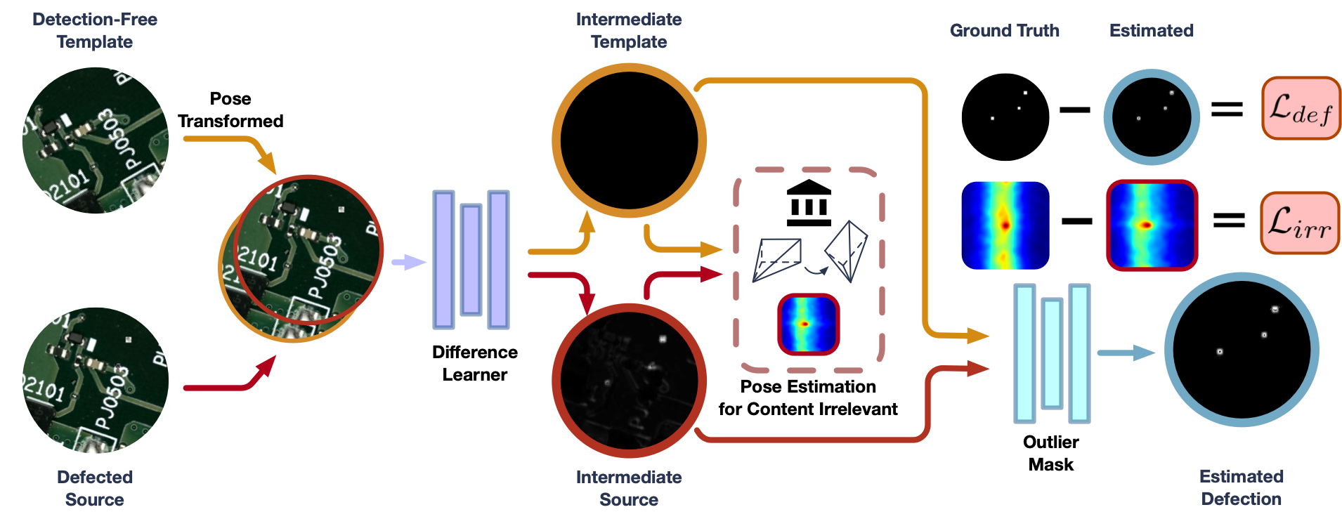
To tackle this challenge, we propose a context insensitive small defection segmentation network which is trained on the simulated environment once for all, named SSDS for “Sim2Real Small Defection Segmentation Network”. SSDS is designed to recognize foreign objects considering two given images who are allowed to also have shifts in space, shown in Fig. 1. The defection-free template is then pose transformed with respect to the pose estimator so that it is pose-aligned to the defected image. To learn to recognize differences between the two images without being misled by the context, a phase correlation based feature extractor is further designed with the backbone of UNet. Utilizing the fact that when two images without share content are fed into deep phase correlation (DPC) [6] to calculate the relative pose, the angle output will give a constant false value at leading to a strong self-supervision constraint forcing the UNet to extract the defection only. Finally, a masking layer further reduces noise introduced by “static shifting” such as assembly error of electronic components in PCB inspection.
The key contribution of the paper is the introduction of guiding a network to distinguish differences between a pair of images to achieve defection segmentation rather than forcing it to remember the context information in the training data. Specific contributions can be summarized as:
-
•
SSDS is proposed to distinguish small defections between an image pair with minimal training data. We guide the network to specifically learn differences between images by making use of the pose sensitivity of phase correlation so that even when trained with cheap simulated data, it can still be generalized to multiple practical applications.
-
•
A new dataset HiDefection [21] containing both generated and actual defections on a PCB board is released for defection segmentation researches and this dataset supports the experiments of the proposed method, which demonstrates superior performance of the generalization ability.
II Related Works
Existing methods for defection detection can be summarized into two fashions: template free and template based. Template free methods usually require one input for detection while template based methods need two: defected image and defection-free template. Each of them has its own share of strength.
II-A Template Free Defection Segmentation
Template free methods can be roughly divided into models based on pretrained feature extractor, generative adversarial network (GAN), and convolutional autoencoder.
Methods based on pretrained feature extractors usually utilize widely adopted feature extractors as well as classifiers. Napoletano et al. [14] utilized ResNet-18 [10] trained on ImageNet [11] to obtain a clustered feature extractor to recognize defections. Andrews et al. [2] achieved the segmentation with the backbone of VGG [18] and utilized a One-Class-SVM [5] to recognize the defection. These methods are limited by the classifier and are gradually replaced by the following generative methods.
GAN based and autoencoder based methods are generative with the assumption that defections should not be generated since they are unseen in the training set. Schlegl et al. [17] proposed a GAN based manifold extractor that was trained on defection free images. It learned a representation of the manifold of the clear images and expecting it to recognize and localize the defections in a defected image. Ackay et al. [1] proposed “Ganomaly” and utilized an autoencoder as the generating part of the GAN following by a decoder to generate a positive image. By comparing the generated image to the input image pixel-wise, defections are expected to be revealed. Bergmann et al. [4] generated positive images with an autoencoder and constructed a specific SSIM loss so that the generative error is related to the pixel-wise similarity. Zhai et al. [20] introduced energy to the regularized autoencoder so the higher energy in the generated output represented the defections. Rudolph et al. [16] detected anomalies via the usage of likelihoods provided by a normalizing flow on multi-scale image features. Comparing to these generative methods, the proposed SSDS adopts the generative fashion but differs in the content of the generated output: SSDS generates the defection directly from the defected and defection-free inputs so that even unseen defections can be recognized.
II-B Template Based Defection Segmentation
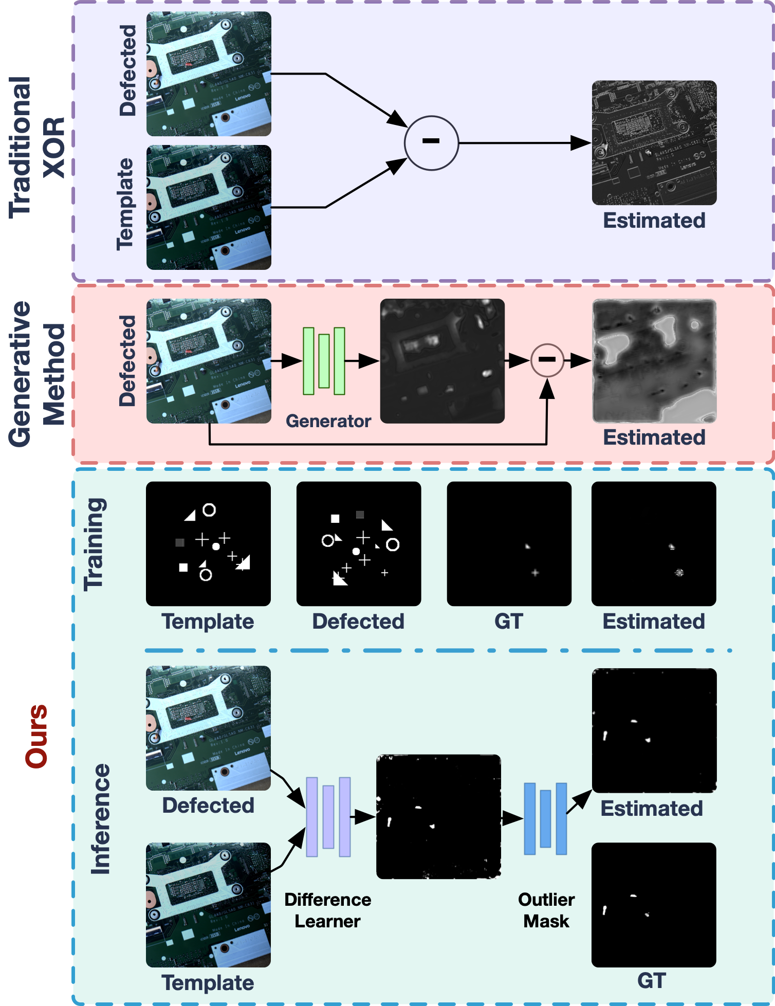
Different from template free approaches, template based methods usually coupe with tiny, vital but untrained defections which can only be recognized by comparing the defected image and the defection-free template. The origin of this is image subtraction [12] by XOR logical operator, it is easy to apply but with extremely high requirements for pixel-wise alignment of the images. Considering this, Ding et al. [8] with feature matching as an improvement has been proposed since it is more robust with pixel errors. Besides feature matching of two images, Gaidhane et al. [9] utilized similarity measurement with symmetric matrix to localize the defection. Although these methods succeeded in detecting tiny untrained defections, they are heavily influenced by the context which means the generalization capability is unsatisfying.
SSDS in this paper aims at detecting those untrained, multi-scaled defections with template based inputs but in a generative way. The proposed method is able to generate defection maps between defected and defection-free images regardless of the context so that it can even be trained in simple simulated data to generalize to multiple practical applications where defection-free template is available.
III Sim2Real Small Defection Segmentation
One typical example of the encountered problem is shown in Fig. 1 where the defected image and the defection free template are the inputs. Since there are multiple mature methods (mechanically as well as algorithmically [6, 7, 13]) that are able to align the images in the industry, we will pass over the pose alignment and assume that the two input images are approximately pose aligned. Following the pipeline in Fig. 2 we design a difference learner for small defection segmentation which aims at only recognizing the differences even if they are small. It is contextual insensitive so that it can be generalized to practical applications with simple training in simulation. Then, a masking module is proposed to eliminate the outlier. Since differentiable pose estimation in plays an important role in the difference learner, we will introduce it as a prerequisite in Section III-A.
III-A Differentiable Phase Correlation
Given two images and with pose transformations, a variation of the deep phase correlator [6] is utilized to estimate the the overall relative pose between and . The rotation and scale is calculated by
| (1) | |||
| (2) |
where is the rotation and scale part of between , is the discrete Fourier Transform, is the log-polar transform, and is the phase correlation solver. Fourier Transformation transforms images into the Fourier frequency domain of which the magnitude has the property of translational insensitivity, therefore the rotation and scale are decoupled with displacements and are represented in the magnitude. Log-polar transformation transforms Cartesian coordinates into log-polar coordinates so that such rotation and scale in the magnitude of Fourier domain are remapped into displacement in the new coordinates, making it solvable with the afterward phase correlation solver. Phase correlation solver outputs a heatmap indicating the displacements of the two log-polar images, which eventually stands for the rotation and scale of the two input images and . To make the solver differentiable, we use expectation as the estimation of .
Then is rotated and scaled referring to with the result of :
| (3) |
With the same manner, translations between and is calculated
| (4) | |||
| (5) |
One unique property of deep phase correlation is to identify whether the two input images are related in content. When and only when the two inputs of the phase correlation in the rotation estimation stage are completely irrelevant, the phase correlation map will be a one-peak distribution centering at exactly [15]. With this property in mind, we will move on to the difference learning module, the difference learning.
III-B Difference Learning
In this module, we aim at designing a learnable layer that can recognize differences between two input images and without being disrupted by the context, and this in the practical applications could be defections in PCB, fingerprints in screen manufacturing, etc.
| (6) |
where is the concatenation, and are the desire outputs of with respect to and . The content of and is further supervised by the proposed “Irrelevance Loss” and by the outlier masking layer introduced in Section III-C.
The “Irrelevance Loss” forces the content of and to be completely different by utilizing the similarity identifying ability of deep phase correlation introduced in Section III-A:
| (7) |
where is the phase correlation result on rotation and scale with respect to and . By expecting and to have completetly irrelevant content, is then supervised by the Kullback–Leibler Divergence loss between the Gaussian Blurred one-peak distribution centering at :
| (8) |
By now the content of and is expected to be completely different from each other. Resulting from this, there are two possibilities for and : i) they are totally in a mess; ii) one of them contains useful information of differences between and . This leads to the next module “Outlier Masking” which also constrains the content of and to be useful.
III-C Outlier Masking
Inspired by the problem in Section III-B, in this module, we define the content of and . We start with focusing on the final defection segmentation result who is derived from the and with a learnable masking layer :
| (9) |
The result should be exactly the same as the ground truth of defection In the coordinate system of , shown as “Defection Estimated” and “Defection GT” in Fig. 1 respectively. Therefore, a hard supervision based on Mean Square Error on and the ground truth is applied:
| (10) |
where is the loss of . The final loss should be:
| (11) |
Since a masking layer cannot generate defections out of nowhere, at least one of and should contain the defection features, However, with introduced (in Section III-B), and must not contain same objects so that the defection features should only be presented in one of them, then we have:
| (12) |
which stands for: there exists exactly one variable in the set that is similar to the output .
To this end, it is clear that one of and is a noisy defection map, but we are not concerned about who exactly it is since they are both intermediate results to be processed by . This explains that the difference learner learns differences between the two input images and that the context is neglected. With the masking layer proposed, the content of and is defined and the segmentation is completed.
III-D Training in Simulation
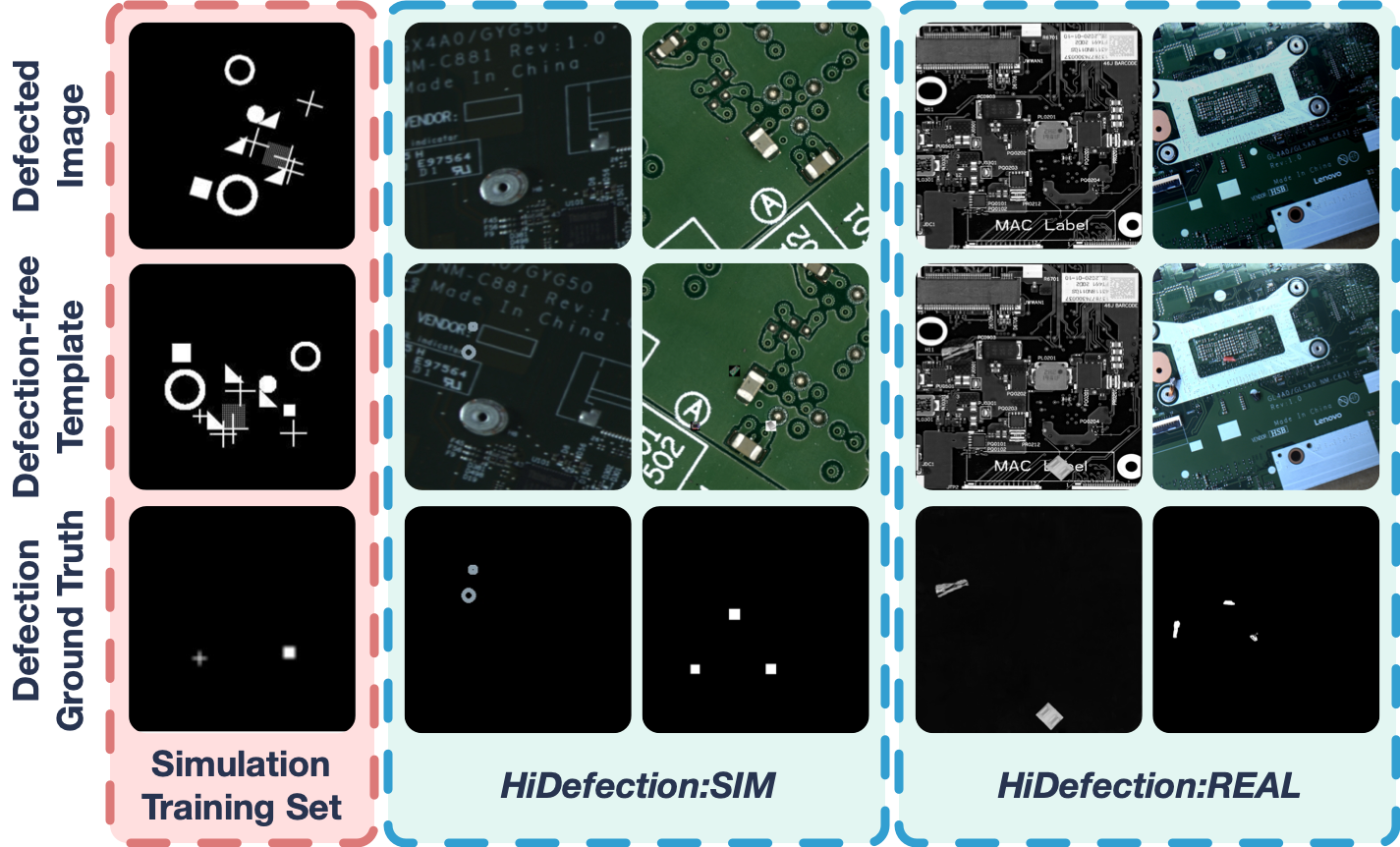
The training skills also play important roles in the methodology since we are designing a once-for-all network needless of further training. One simulated dataset is specifically designed for the SSDS’s training with randomization, shown in Fig. 3 (Simulation Training Set). One defection-free template is firstly generated with a random number of random shapes at random locations. For the defected image, comparing to the defection-free one, the same number of same shapes are generated around the same location with slight random translational disturbance for imitating practical usage, e.g. assembly error of electronic components. Then the generated defected image is rotated and scaled randomly to simulate the overall pose misalignment in practical applications. The simulated data is completely randomized so that the network will not overfit and will focus on the difference learning. Note that the shapes are partially borrowed from [3].
IV Experiments: Dataset And Setup
Our method is trained in simulation (Fig. 3: Simulation Training Set) and evaluated on the sim&real dataset HiDefection [21] for PCB defection segmentation. As one of the contributions of this paper, HiDefection contains two packages HiDefection:SIM and HiDefection:REAL. HiDefection:SIM is constructed with randomly generated shapes as defections on two different types of PCBs as background and HiDefection:REAL with realistic photos of actual objects on PCBs.
IV-A Dataset
HiDefection: The HiDefection is a real-world dataset collected both in a PCB workshop with simulated defections in different types of PCB and actual defected boards together with their corresponding defection-free templates.
-
•
HiDefection:SIM: It is recorded in the overhead perspective of a large amount of PCBs and is leveraged in the paper. The random defections in this part of dataset contain random shapes and randomly dropped electronic components. Defections are small with the largest being of the whole image. The total size of this part of dataset is 15000 pairs for training and 3000 pairs for validation. One sample pair is shown in Fig. 3 as “HiDefection:SIM”.
-
•
HiDefection:REAL: This sub-dataset is recorded in the same camera condition with HiDefection:SIM above but with real defections and PCBs shot together so that it can represent what defection segmentation actually encounters in real-world applications. When collecting, we also introduce light changes in some pairs of images to make it more realistic so that the result on this can be representative of what one method will achieve in practice. Moreover, the assembly error of electronic components are introduced to every pair of data which makes the small defection segmentation more challenging. Note that the size of the largest defection in this part of data will not exceed of the whole image. This part of dataset is designed for validating the generalizing ability of defection segmentation methods and contains 100 pairs of images. One sample pair is shown in Fig. 3 as “HiDefection:REAL”.
| Scene | Baselines |
|
|
||||||
|---|---|---|---|---|---|---|---|---|---|
| AP() | MaxF1() | AP() | MaxF1() | ||||||
| I | GANomaly | 98.2 | 97.5 | 45.4 | 43.1 | ||||
| SSIM | 97.2 | 98.7 | 38.7 | 39.4 | |||||
| DSEBM | 98.1 | 94.3 | 28.9 | 42.5 | |||||
| TDD-net | 98.4 | 98.6 | 50.3 | 67.1 | |||||
| SSDS | 97.4 | 95.5 | |||||||
| II | GANomaly | 96.3 | 95.2 | 22.4 | 27.3 | ||||
| SSIM | 97.0 | 93.4 | 40.3 | 29.9 | |||||
| DSEBM | 98.4 | 97.0 | 30.5 | 45.2 | |||||
| TDD-net | 95.6 | 97.7 | 42.9 | 33.5 | |||||
| SSDS | 97.8 | 98.2 | |||||||
For all dataset above, defected images are pose transformed from the defection-free template with the constraint on translations of both and , rotation changes and scale changes of the two images in the range of pixels, and respectively with images shapes of .
IV-B Metrics
We evaluate the performance of the defection segmentation with Intersection-over-Union(IoU) AP, Recall Rate R and the Harmony Mean(MaxF1) of AP and R. In Section V, AP and MaxF1 are adopted for quantitative demonstration.
IV-C Comparative Methods
Baselines in the experiment include template free methods GANomaly[1], SSIM [4], DSEBM[20] and template based method TDD-net [8]. All the comparative methods share the same training condition and are trained in the simulated dataset and on HiDefection. They are evaluated on HiDefection as comparisons to prove the generalization capability of SSDS.
| Scene | Baselines |
|
|
||||||
|---|---|---|---|---|---|---|---|---|---|
| AP() | MaxF1() | AP() | MaxF1() | ||||||
| III | GANomaly | 19.9 | 23.1 | 21.0 | 18.7 | ||||
| SSIM | 11.1 | 29.3 | 12.9 | 21.1 | |||||
| DSEBM | 11.9 | 26.2 | 20.5 | 17.5 | |||||
| TDD-net | 19.2 | 23.8 | 21.4 | 21.9 | |||||
| SSDS | 98.1 | 96.3 | |||||||
| IV | GANomaly | 10.6 | 17.1 | 11.0 | 16.9 | ||||
| SSIM | 13.5 | 12.9 | 16.2 | 20.1 | |||||
| DSEBM | 26.7 | 21.5 | 39.2 | 43.1 | |||||
| TDD-net | 33.6 | 19.2 | 29.0 | 31.5 | |||||
| SSDS | 97.1 | 94.7 | |||||||
V Experiments: Results
V-A PCB with Simulated Defection
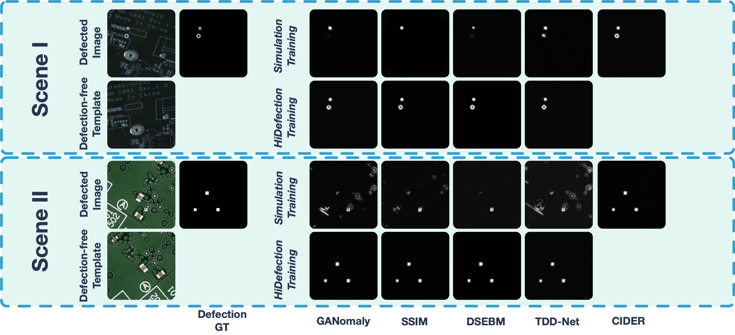
In this experiment, we evaluate SSDS on HiDetection:SIM where “Scene I” has simulated shapes on PCBs and “Scene II” has randomly placed electronic components on PCBs. We train SSDS and the rest of the baselines in simulation and test it on HiDetection:SIM. However, to prove the generalization capability, we additionally train all baselines in HiDetection:SIM except for SSDS. The qualitative result shown in Fig. 4 and the quantitative result in TABLE. I demonstrate the superior performance SSDS achieved in generalizing simulation training to practical inference and it outperforms other baselines in generalizing. Even when trained in simulation with a completely different context, SSDS could still be on par with baselines that are trained on HiDetection:SIM when comparing the performance on inferring defections of PCBs. When inferred in a different context from training, template free and generative baselines (GANomaly, SSIM, DSEBM) are easily confused by the new context and inevitably miss important defections, and template based baseline TDD-net is misled by the assembly error of the components so that its output is blurry.
In the HiDetection:SIM where defections are simulated and are similar to what they are in the simulated training, baselines’ generalizing ability is still worthy of segmentation. However, when defections are from the real world, their performances start to drop, and this leads to Section V-B.
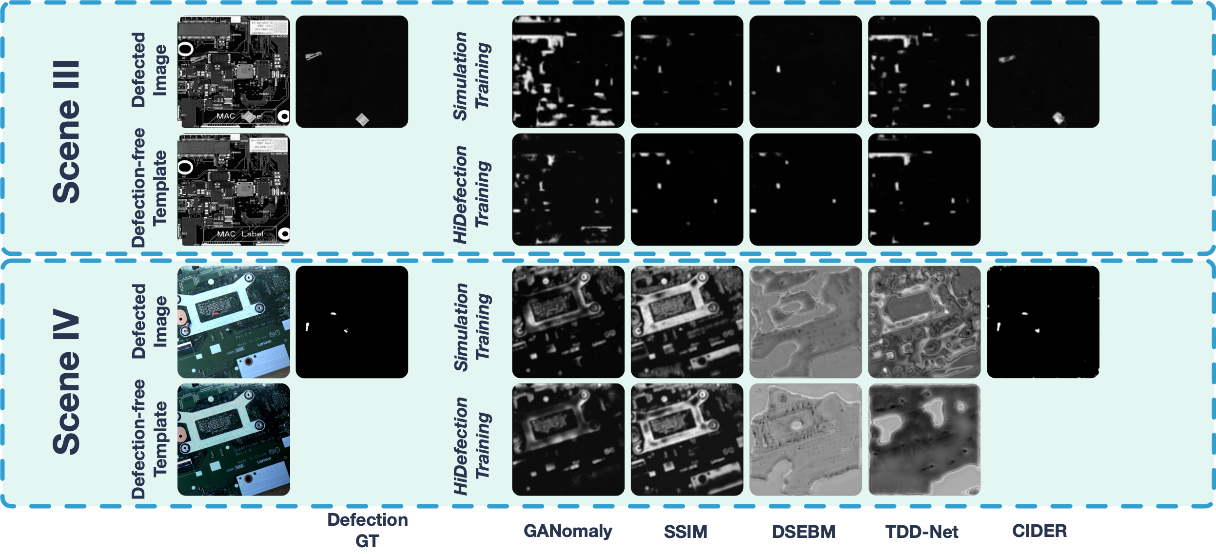
V-B PCB with Real Defection
In this experiment, we evaluate SSDS on HiDefection:REAL where “Scene III” and “Scene IV” are both real-world particles and PCBs with lighting changes. Different from what has been conducted in Section V-A, all methods including SSDS have not been trained on HiDefection:REAL so that the generalization is further studied. The qualitative result is shown in Fig. 5 and the quantitative result is shown in TABLE. II. The result indicates that with defections from the real world involved which have not been seen in any of the training data, both the comparing methods trained in simulation and trained in HiDefection:SIM fail to present successful predictions of the defection. In contrast, SSDS trained in simulation is still a competent approach to recognize defection, even when light changes are involved in one pair of images. This proves the generalizing ability of SSDS and that the method can be directly adopted in practical applications without any further training.
V-C Ablation Study
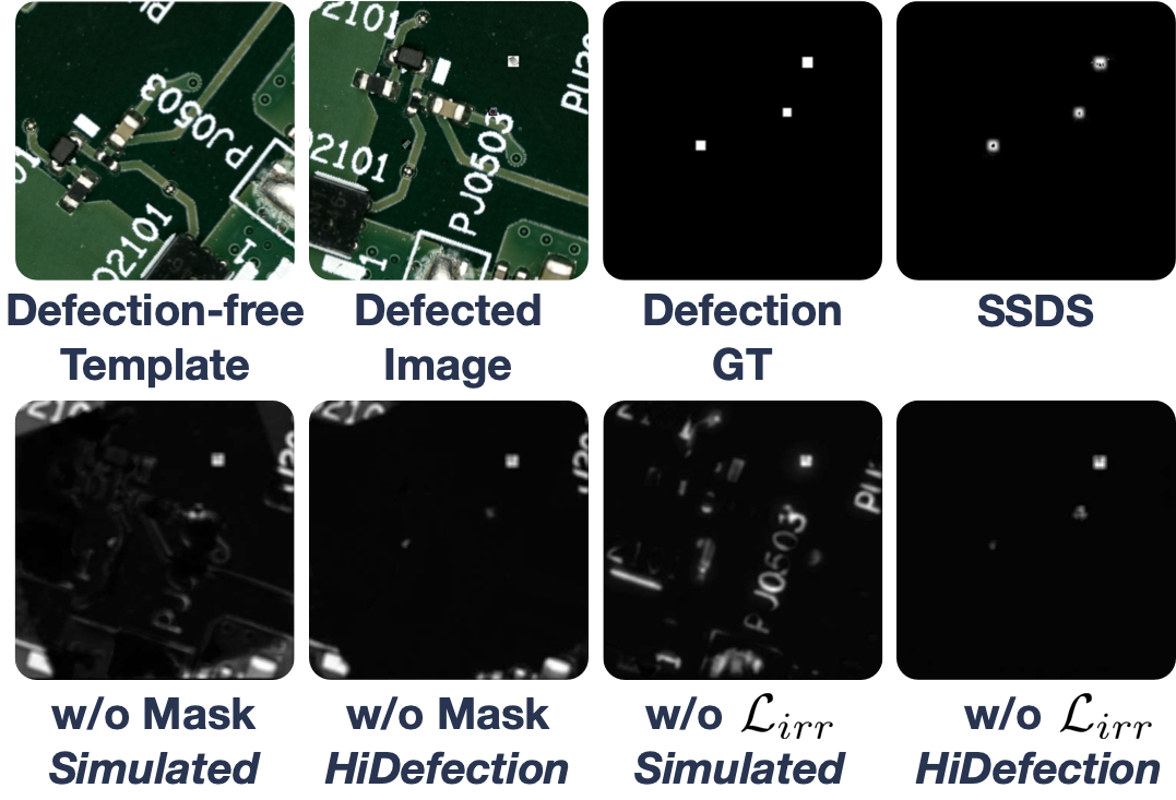
Several experiments are designed for ablation studies to reassure that each module involved plays its own important role. Firstly, we validate the role of the difference learning layer by deprecating this layer and the corresponding loss in the training stage(denotes as “w/o ”). In such study, “w/o ” is trained both in simulation and on HiDefection and evaluated in HiDefection. The qualitative result (Fig. 6) and the quantitative result (TABLE. III) shows that while “w/o ” trained on HiDefection still gives a satisfying result, it fails in defection segmentation when it is trained in the simulation. This proves that, without the difference learning layer, the method will still work when the training and inferring share the same context, but will fail when they are different. It also proves that the difference learning layer is a vital component for the context insensitive behavior.
We further study the importance of the masking layer by deprecating such layer and calculate the defection MSE loss directly between and (denotes as “w/o Mask”). The qualitative result (Fig. 6) and the quantitative result (TABLE. III) shows that “w/o Mask” trained on both HiDefection and simulation is able to provide acceptable results in but with more noise generated from the assembly error on components. This proves that the masking layer efficiently eliminates the unfavorable noise due to pixel error.
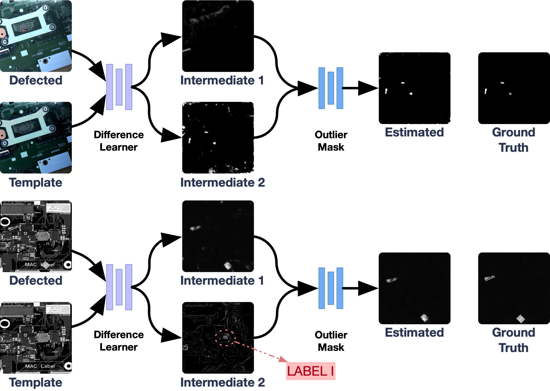
V-D Case Study
We visualize the intermediate results in the whole method to prove our interpretation of the network, shown in Fig. 7. The first case (upper case in Fig. 7) is conducted on a set of PCBs images shot in different lighting conditions, and the second case (lower case in Fig. 7) is where the shapes of silicon grease varies from each other but should not be counted as defection. We trained the network twice in simulation resulting in two independent models. The first model have the “Intermediate 2” generated with defections while the second model have it in “Intermediate 1”. It proves that one of the two outputs of the “Difference Learner” contains specific defections with noise introduced by pixel-wise error of the two images and the “Outlier Mask” is able to filter the noise out.
While it is satisfying to prove that SSDS is able to deal with lighting changes, its potential of handling images with false defections is rewarding. Note that in the second case, when defections are presented in “Intermediate 1”, the differences in silicon grease is presented in “Intermediate 2” and is filtered out after the “Outlier Mask”.
| Ablation |
|
|
|||||||
|---|---|---|---|---|---|---|---|---|---|
| w/o | w/o Mask | w/o | w/o Mask | SSDS | |||||
| AP() | 59.1 | 77.8 | 17.9 | 72.5 | 97.8 | ||||
| MaxF1() | 63.4 | 74.2 | 19.3 | 78.1 | 98.2 | ||||
VI Conclusion
We present an approach for small defection segmentation with simple training in simulated environment, namely SSDS. To achieve this, we design one difference learner based on the deep phase correlation so that it can recognize defections regardless of the context, and one masking layer for outlier elimination. In various experiments, the proposed SSDS presents satisfying performances in generalization, i.e. background changes and lighting changes, showing its potential for practical defection segmentation application.
References
- [1] Samet Akcay, Amir Atapour-Abarghouei and Toby P Breckon “Ganomaly: Semi-supervised anomaly detection via adversarial training” In Asian conference on computer vision, 2018, pp. 622–637 Springer
- [2] Jerone Andrews, Thomas Tanay, Edward J Morton and Lewis D Griffin “Transfer representation-learning for anomaly detection”, 2016 JMLR
- [3] Anonymous URL: https://github.com/usuyama/pytorch-unet
- [4] Paul Bergmann et al. “Improving unsupervised defect segmentation by applying structural similarity to autoencoders” In arXiv preprint arXiv:1807.02011, 2018
- [5] Yunqiang Chen, Xiang Sean Zhou and Thomas S Huang “One-class SVM for learning in image retrieval” In Proceedings 2001 International Conference on Image Processing (Cat. No. 01CH37205) 1, 2001, pp. 34–37 IEEE
- [6] Zexi Chen, Xuecheng Xu, Yue Wang and Rong Xiong “Deep Phase Correlation for End-to-End Heterogeneous Sensor Measurements Matching” In arXiv preprint arXiv:2008.09474, 2020
- [7] Jiaxin Cheng, Yue Wu, Wael AbdAlmageed and Premkumar Natarajan “QATM: Quality-aware template matching for deep learning” In Proceedings of the IEEE/CVF Conference on Computer Vision and Pattern Recognition, 2019, pp. 11553–11562
- [8] Runwei Ding, Linhui Dai, Guangpeng Li and Hong Liu “TDD-net: a tiny defect detection network for printed circuit boards” In CAAI Transactions on Intelligence Technology 4.2 IET, 2019, pp. 110–116
- [9] Vilas H Gaidhane, Yogesh V Hote and Vijander Singh “An efficient similarity measure approach for PCB surface defect detection” In Pattern Analysis and Applications 21.1 Springer, 2018, pp. 277–289
- [10] Kaiming He, Xiangyu Zhang, Shaoqing Ren and Jian Sun “Deep residual learning for image recognition” In Proceedings of the IEEE conference on computer vision and pattern recognition, 2016, pp. 770–778
- [11] Alex Krizhevsky, Ilya Sutskever and Geoffrey E Hinton “Imagenet classification with deep convolutional neural networks” In Advances in neural information processing systems 25, 2012, pp. 1097–1105
- [12] Madhav Moganti and Fikret Ercal “Automatic PCB inspection systems” In IEEE Potentials 14.3 IEEE, 1995, pp. 6–10
- [13] Muhammad Hamza Mughal, Muhammad Jawad Khokhar and Muhammad Shahzad “Assisting UAV Localization via Deep Contextual Image Matching” In IEEE Journal of Selected Topics in Applied Earth Observations and Remote Sensing IEEE, 2021
- [14] Paolo Napoletano, Flavio Piccoli and Raimondo Schettini “Anomaly detection in nanofibrous materials by CNN-based self-similarity” In Sensors 18.1 Multidisciplinary Digital Publishing Institute, 2018, pp. 209
- [15] Alan V Oppenheim and Jae S Lim “The importance of phase in signals” In Proceedings of the IEEE 69.5 IEEE, 1981, pp. 529–541
- [16] Marco Rudolph, Bastian Wandt and Bodo Rosenhahn “Same same but differnet: Semi-supervised defect detection with normalizing flows” In Proceedings of the IEEE/CVF Winter Conference on Applications of Computer Vision, 2021, pp. 1907–1916
- [17] Thomas Schlegl et al. “Unsupervised anomaly detection with generative adversarial networks to guide marker discovery” In International conference on information processing in medical imaging, 2017, pp. 146–157 Springer
- [18] Karen Simonyan and Andrew Zisserman “Very deep convolutional networks for large-scale image recognition” In arXiv preprint arXiv:1409.1556, 2014
- [19] Yue Wang, Shoudong Huang, Rong Xiong and Jun Wu “A framework for multi-session RGBD SLAM in low dynamic workspace environment” In CAAI Transactions on Intelligence Technology 1.1 Elsevier, 2016, pp. 90–103
- [20] Shuangfei Zhai, Yu Cheng, Weining Lu and Zhongfei Zhang “Deep structured energy based models for anomaly detection” In International Conference on Machine Learning, 2016, pp. 1100–1109 PMLR
- [21] ZJU-Robotics-Lab “HiDefection Dataset”, 2020 URL: https://github.com/ZJU-Robotics-Lab/OpenDataSet