Learn to Rapidly and Robustly Optimize Hybrid Precoding
Abstract
Hybrid precoding plays a key role in realizing massive multiple-input multiple-output (MIMO) transmitters with controllable cost. MIMO precoders are required to frequently adapt based on the variations in the channel conditions. In hybrid MIMO, where precoding is comprised of digital and analog beamforming, such an adaptation involves lengthy optimization and depends on accurate channel state information (CSI). This affects the spectral efficiency when the channel varies rapidly and when operating with noisy CSI. In this work we employ deep learning techniques to learn how to rapidly and robustly optimize hybrid precoders, while being fully interpretable. We leverage data to learn iteration-dependent hyperparameter settings of projected gradient sum-rate optimization with a predefined number of iterations. The algorithm maps channel realizations into hybrid precoding settings while preserving the interpretable flow of the optimizer and improving its convergence speed. To cope with noisy CSI, we learn to optimize the minimal achievable sum-rate among all tolerable errors, proposing a robust hybrid precoding based on the projected conceptual mirror prox minimax optimizer. Numerical results demonstrate that our approach allows using over ten times less iterations compared to that required by conventional optimization with shared hyperparameters, while achieving similar and even improved sum-rate performance.
I Introduction
Wireless communication networks are subject to constantly growing requirements in terms of connectivity, throughput, and reliability. One of the emerging technologies which is expected to play a key role in meeting these demands is based on equipping wireless base stations with large-scale antenna arrays, resulting in massive MIMO networks [2]. While the theoretical gains of massive MIMO are well-established [3, 4, 5], implementing such large scale arrays in a power and cost efficient manner is associated with several core challenges. Among these challenges is the conventional need to feed each antenna element with a dedicated RF chain, which tend to be costly and consume notable power [6].
A leading approach to tackle the cost and power challenges of massive MIMO is to utilize hybrid analog/digital MIMO transceivers [7, 8]. Hybrid MIMO transceivers carry out part of the processing of the transmitted and received signals in the analog domain, enabling operation with less RF chains than antennas [9, 10, 11]. As a result, hybrid MIMO transmitters implement precoding partially in digital and partially in analog. Analog processing is dictated by the circuitry, often implemented using vector modulators [12] or phase shifters [9]. Consequently, analog precoding is typically more constrained compared with digital processing, where, e.g., one can typically apply different precoders in each frequency [13].
The constrained form of hybrid MIMO makes the setting of the precoding pattern for a given channel realization notably more challenging compared with costly fully-digital architectures. Various methods have been proposed for designing hybrid precoding systems, optimizing their analog and digital processing to meet the communication demands [14]. The common approach formulates the objective of the precoders, e.g., sum-rate maximization or minimizing the distance from the fully-digital precoder [15, 16], as an optimization problem. The resulting optimization is then tackled using iterative solvers which vary based on the objective and the specific constraints induced by the analog circuitry and the antenna architecture. Iterative algorithms were proposed for tunning hybrid MIMO systems with controllable gains [11], phase-shifting structure [10, 13], partial-connectivity [9, 15], discretized vector modulators [12], and Lorentzian-constrained metasurface antennas [17, 18]. While iterative optimizers are interpretable, being derived as the solution to the formulated problem, they are often slow in terms of convergence. This can be a major limitation as this setting is based on the instantaneous CSI, and thus must be done in real-time to cope with the frequent variations of wireless channels, and its performance depends on the accuracy of the CSI.
An alternative emerging approach to tuning hybrid precoders is based on deep learning. This approach builds upon the ability of deep neural networks to learn complex mapping while inferring at controllable speed dictated by the number of layers, which is often much faster compared with conventional iterative optimizers [19]. The usage of deep learning to tackle optimization problems is referred to as learn-to-optimize [20]. DNN-aided optimization of hybrid precoders was considered in [21, 22, 23, 24, 25, 26, 27], which employed multi-layered perceptrons [21, 22] and convolutional neural networks [23, 24, 25, 26, 27] as the optimizer, while [28, 29] employed deep reinforcement learning techniques. While such deep models are able to map channel estimates into precoder structure, they lack of transparency or interpretability in how input data are transformed into the precoder setting. Furthermore, the resulting precoding scheme is geared towards the number of users and the distribution of the channels used for its training. When the channel distribution or the number of users changes, the DNN needs to be trained anew, which is a lengthy procedure. Moreover, highly-parameterized DNNs may be too computationally complex to deploy on hardware-limited wireless communication devices.
Interpretable deep models with a small number of parameters can be obtained from iterative optimization algorithms via the deep unfolding methodology [30]. Deep unfolding leverages data-driven deep learning techniques to improve an iterative optimizer, rather than replace its operation with DNNs [31, 32]. Deep unfolded optimizers were utilized for configuring one-bit hybrid precoders in [33]; for fully-digital (non-hybrid) narrowband precoders in [34]; for narrowband phase shifter based hybrid precoders in [35, 36]; and for narrowband hybrid predcoders with limited feedback in [37]. The latter unrolled an optimization algorithm using generative networks for handling the limited feedback and overparametrized ResNets for optimizing the precoders, resulting in a highly-parameterized DNN, which may not be suitable for application on hardware limited MIMO devices. The work [38] used dedicated DNNs integrated into unfolded optimization of analog precoders in hybrid MIMO transmitters with full CSI, at the cost of additional complexity during inference. This motivates designing interpretable light-weight learn-to-optimize algorithms for rapidly translating CSI into multi-band hybrid precoders, while being robust to inaccurate CSI.
In this work, we propose a learn-to-optimize algorithm for tuning multi-band downlink hybrid MIMO precoders in a manner that is rapid, robust, and interpretable. We consider different analog architectures, including analog precoders with controllable gains, as well as architectures based on fully-connected phase shifters. Our approach leverages data in the form of past channel realization to accelerate the convergence of conventional iterative optimization of the achievable sum-rate. In order to design an unfolded algorithm for dealing with the challenging and practical setting where the CSI may be noisy, we commence by treating the setting where full CSI is available, for which we formulate an unfolded optimizer which naturally extends to cope with noisy CSI. Our proposed data-aided algorithms fully preserve the interpretable and flexible operation of conventional optimizers from which they originate, while being light-weight and operating with fixed run-time and complexity.
In particular, we adopt the projected gradient ascent (PGA) algorithm as the hybrid precoding designing optimizer for maximizing the achievable sum-rate with full CSI. Our motivation here stems from the ability of this approach to directly optimize the sum-rate, rather than adopting some simpler surrogate objective as done in, e.g., [15, 10], which can thus be extended to robust optimization of this measure. We unfold the PGA algorithm, by fixing a small number of iterations and train only its iteration-dependent hyperparameters which can be tuned from data without deviating from its overall flow and operation.
Our selection of PGA optimization with the sum-rate objective as our basis for hybrid precoding design with full CSI facilitates extending our approach to noisy CSI settings: we identify the projected conceptual mirror prox (PCMP) algorithm for maximin optimization [39] as a suitable optimizer for hybrid precoding with noisy CSI, whose algorithmic steps involve computations of gradients of projection of the sum-rate objective, as we used by PGA with full CSI. Consequently, we propose to cope with noisy CSI by formulating our design objective as maximizing the minimal achievable sum-rate within a given tolerable CSI error margin. We then unfold PCMP, resulting in a trainable architecture involving similar steps as those used when unfolding PGA, where again data is leveraged to tune the hyperparameters of the optimizer for each iteration. Our experimental results evaluate our proposed unfolded algorithms compared with the conventional optimizers from which they originate for hybrid precoding in multi-band synthetic Rayleigh channels as well as channels generated via the Quasi Deterministic Radio channel Generator (QuaDRiGa) channel simulator [40] in various signal-to-noise ratios. There, we systematically show that the proposed unfolded algorithms achieve similar and even improved sum-rates compared with their iterative counterparts, while operating with over ten times less iterations and computational complexity.
The rest of this work is organized as follows: Section II describes the system model; the proposed learn-to-optimize algorithm for tuning hybrid precoders with full CSI is derived in Section III, while Section IV derives the learned optimizer for noisy CSI. Our proposed algorithms are numerically evaluated in Section V, and Section VI provides concluding remarks.
Throughout the paper, we use lowercase boldface letters for vectors, e.g., ; denotes the th element of . Uppercase boldface letters are used for matrices, e.g., , with being its th entry and denoting the identity matrix. Calligraphic letters, such as , are used for sets, and is the set of complex numbers. The transpose, Hermitian transpose, Frobenius norm, and stochastic expectation are denoted by , , , and , respectively.
II System Model
In this section we present the system model. We start by reviewing the model for wideband downlink MIMO communications with hybrid beamforming in Subsection II-A, after which we discuss the considered analog precoder architectures in Subsection II-B. Then, we formulate the considered problem of rapid and robust hybrid precoder setting in Subsection II-C.
II-A Downlink MIMO Communications with Hybrid Beamforming
II-A1 Channel Model
We consider a single-cell downlink hybrid MIMO system with single-antenna users. The BS is equipped with transmitting antennas, and utilizes frequency bands for communications, where the spectrum is shared among all users in a non-orthogonal fashion. The overall system is illustrated in Fig. 1.
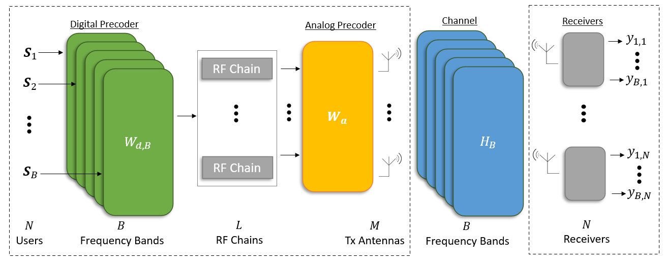
The BS employs multi-carrier signaling, and we use to denote the multiuser transmitted signal vector that is being transmitted in the th frequency bin, . The transmitted symbols are i.i.d. and of equal power, such that for each . At each frequency bin , for a channel input , the channel output is given by
| (1) |
where is the th frequency band sub-channel, and is additive white Gaussian noise (AWGN) with i.i.d. entries of variance .
II-A2 Hybrid Beamforming
The BS has RF chains, and thus employs hybrid precoding. Here, the multiuser transmitted signal vectors are precoded in two stages. First, a digital precoder is applied to in each frequency bin , i.e., is the digital precoding matrix of the th bin. Next, the digital symbols pass through RF chains, and are combined into the channel input using an analog precoder. Unlike digital processing, analog precoding is carried out using dedicated hardware assumed to be static in frequency. Hence, analog precoding is modeled using the matrix , where represents the set of feasible analog precoder settings, discussed in the sequel.
II-B Analog Precoders
The feasible mappings that can be realized by the analog precoder , encapsulated in the set , depend on the hardware architecture. We consider two different architectures for the analog precoder: unconstrained precodersZ and fully-connected phase shifter networks.
II-B1 Unconstrained Precoder
Here, the analog precoding matrix, , has no hardware constraints, and can realize any complex matrix (while satisfying the overall power constraint (3)). For unconstrained precoders, we use . Such analog processing with configurable attenuation and phase shifting can be implemented using, e.g., vector modulators, as in [11, 12]. While this formulation does not assume any constraints, other than the power constraint, it is emphasized that unconstrained solutions can be useful for constrained analog hardware designs, which often involve a preliminary step of obtaining an unconstrained combiner followed by its projection to the constrained set, as done in, e.g., [10].
II-B2 Phase Shifter Networks
A common implementation of analog precoders utilizes phase shifters [10, 9]. In fully-connected phase shifter networks, every antenna element is connected to each RF chain via a dedicated controllable phase shifter. Such precoders are modelled as matrices whose entries have a unit magnitude, namely,
| (5) |
II-C Problem Formulation
We aim at designing the hybrid precoding operation given a channel realization to maximize the achievable sum-rate of multiuser downlink MIMO communications. Defining the sum-rate as the precoding objective is a common approach [18, 41, 13], being a communication measure of the overall combined effect of the channel and the hybrid precoder. We particularly focus on two scenarios – sum-rate maximization (given accurate CSI) and robust sum-rate maximization (given noisy CSI).
II-C1 Sum-Rate Maximization
Since , it holds that the following sum-rate is achievable [42]
| (6) |
Consequently, for a given channel realization , we aim to find and , that are the solution to the following optimization problem
| (7) | ||||
In (7), is the set of matrices corresponding to the analog precoding models described above, i.e., we seek to find a suitable precoders under the different constraints detailed in Subsection II-B.
Since the optimization problem (7) must be tackled each time the channel realization changes, our proposed solution should not only tackle (7), but also to do it rapidly, i.e., with a predefined amount of computations. To achieve this aim, we assume access to a set of previously encountered or simulated channel realizations , which can be exploited to facilitate optimization within a fixed number of operations (dictated by, e.g., the coherence duration of the channel).
II-C2 Robust Sum-Rate Maximization
The optimization problem in (7) relies on knowledge of the channel in each frequency bin, i.e., on full CSI. Using (6) as our objective is expected to affect the performance of the hybrid precoders when the channel matrices provided as inputs are (possibly inaccurate) estimates of the true channel. Consequently, we seek to optimize the hybrid precoders in a manner that is robust to a predefined level of inaccuracies in the CSI.
To formulate this, we consider a noisy sub-channel estimation denoted , where is the true channel realization, and is the estimation error. We wish to design the hybrid precoders to be robust to estimation errors within a predefined level , i.e., when for each . Consequently, we convert (7) into a maximin problem
| (8) | ||||
In (8), we seek to maximize the minimal rate resulting from a tolerable estimation error of the channel, i.e., an estimation error within the predefined level . Again, we wish to carry out robust optimization rapidly, and can leverage the set of past channel realizations to that aim.
III Rapid Hybrid Precoder Learned Optimization with Full CSI
We first consider the rapid tuning of the hybrid precoder with full CSI. For each realization of the wireless channel , the configuration of the hybrid precoder can be formulated as a constrained optimization problem (7). Consequently, one can design a hybrid precoder using suitable iterative optimization methods. A candidate method for tackling the optimization problem in (7) is PGA. PGA can directly tackle the multi-carrier sum-rate objective in (7), as opposed to alternative iterative optimizers for hybrid beamforming which use a relaxed objective aiming to approach the fully-digital beamformer as in [15, 10]. An additional motivation for aiming at directly optimizing the sum-rate rather than an alternative surrogate objective (which may be desired to optimize) stems from the fact that the resulting derivation can be extended to robust optimization, i.e., to cope with noisy CSI, as detailed in Section IV. Setting the hybrid precoder setup is a channel-dependent task. Consequently, one would have to carry out the optimization procedure each time the channel changes, i.e., on each coherence duration, while principled iterative optimizers such as PGA tend to be slow and lengthy. To cope with this challenge, in this section we present the method of learn-to-optimize hybrid precoding with full CSI, which is specifically designed to rapidly configure hybrid precoders. Our scheme is based on the application of PGA to (7), as detailed in Subsection III-A, whose convergence speed we optimize without compromising on interpretability and suitability using deep unfolding [31], as we derive in Subsection III-B and discuss in Subsection III-C.
III-A Projected Gradient Ascent
Problem (7) represents constrained maximization with optimization matrix variables . Such problems can be tackled using the PGA algorithm combined with alternating optimization. In this iterative method, each iteration first optimizes while keeping fixed, then repeats this process for every . The optimized matrices are projected to guarantee the constraints are not violated.
To formulate this operation mathematically, we define . Each iteration of index is comprised of two alternating stages: analog PGA and digital PGA.
Analog PGA: The update of is carried out according to
| (9) |
where is the step size of the gradient step, and is the projection operator onto the set . The gradient of R with respect to is given by (see Appendix A)
| (10) |
where .
The projection operator in (9) depends on the feasible analog mappings. For unconstrained architectures, clearly . For fully connected phase shifters based hardware, the projection is given by
| (11) |
Digital PGA: The digital precoder is updated after the analog precoder, where the update is carried out for all frequencies in parallel. Namely, the gradient step for each is computed as
| (12) |
where is the step size. The gradient of R with respect to for each is computed as (see Appendix A)
| (13) |
After the gradient step is taken for all frequency bins, the solution is projected to meet the power constraint via
| (14) |
The overall procedure is summarized as Algorithm 1. While the initial settings of are taken to be random, the initial analog combiner is set to be the first right-singular vectors of (the frequency bands sub-channels average). This setting corresponds to analog beamforming towards the eigenmodes of the (frequency-average) channel, being the part of the capacity achieving precoding method for frequency flat MIMO channels [43, Ch. 10]. This principled initialization is numerically shown to notably improve the performance of hybrid precoders tuned to directly optimize the rate in (7).
first right-singular vectors of
Set step sizes
The convergence speed of gradient-based optimizers largely depends on the step sizes, i.e., in Algorithm 1. However, conventional step size optimization methods based on, e.g., line search and backtracking [44, Ch. 9], typically involve additional per-iteration processing which increases the overall complexity and run-time. Hence, a common practice is to use pre-defined hand-tuned constant step sizes, which may result in lengthy convergence.
III-B Learn-to-Optimize Hybrid Precoding
Algorithm 1 optimizes hybrid precoders for a given channel realization. However, its convergence speed largely depends on its hyperparameters, i.e., the step sizes, which tend to be difficult to set. Here, we propose to leverage automated data-based optimizers used in deep learning to tune iteration-dependent step sizes, i.e., to learn-to-optimize hybrid precoders in a small and predefined number of iterations.
Our design follows the deep unfolding methodology [30, 31], which designs DNNs as iterative optimizers with a fixed number of iterations. In particular, we use as our optimizer the PGA method in Algorithm 1 with exactly iterations. By doing so, we guarantee an exact pre-known, and typically small, run-time and complexity in real-time. While the accuracy of first-order optimizers such as PGA is typically invariant of the setting of the hyperparameters when allowed to run until convergence (under mild conditions, e.g., that the step sizes are sufficiently small), their performance is largely affected by these values when the number of iterations is fixed. Consequently, our design treats the hyperparameters of an iterative optimizer with iterations as the parameters of a DNN with layers, and tunes them via end-to-end training, based on the available data set , thus converting PGA into a trainable discriminative model [45].
To formulate this, the step sizes vector of the th iteration is defined as , and the step sizes matrix defined as for iterations of Algorithm 1. The entries of this matrix are trainable parameters, that are learned from data. Note that end-to-end training is feasible despite the fact that does not hold the ground truth precoders. This follows since the performance of hybrid precoders can be evaluated using the differentiable measure in (6), that is used to define a loss function with which the hyperparameters are trained in an unsupervised manner.
The loss function, for a given normalized channel and step sizes , is computed as a weighted average of the negative resulting achievable sum-rates of this channel (6) in each iteration. This implies that the th iteration sum-rate is computed when the precoders are , i.e., the precoders obtained via Algorithm 1 after iterations and step sizes . Since each iteration is required to provide a setting of the hybrid beamformer which gradually improves along the iterative procedure, we adopt the following loss, inspired by [46]
| (15) |
The data set includes channel realizations. Since with known and , we henceforth write the entries of the data set as .
The learn-to-optimize method seeks to tune the hyperparameters vector to best fit the data set in the sense of the loss measure (15). Namely, we aim at setting
| (16) |
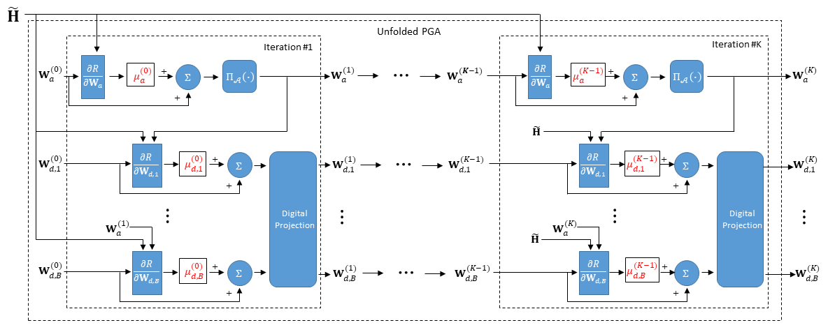
We tackle (16) using deep learning optimization techniques based on, e.g., mini-batch stochastic gradient descent, to tune based on the data set . The resulting procedure is summarized as Algorithm 2. We initialize before the training process, with fixed step sizes with which PGA converges. After training, which is based on past channel realization and can thus be done offline, the learned is used as hyperparameters for rapidly converting a channel realization into a hybrid precoding setting via of Algorithm 1. The resulting unfolded PGA algorithm is illustrated in Fig. 2.
Fix learning rate
III-C Discussion
The proposed learn-to-optimize method leverages data to improve the performance and convergence speed of iterative PGA-based optimization. The resulting precoder design preserves the interpretability and simplicity of classic PGA optimization, while inferring at a fixed and low delay as done by DNNs applied for such tasks. We thus benefit from the best of both worlds of model-based optimization and data-driven deep learning.
The fact that the number of iterations is fixed and limited is reflected upon the computational complexity associated with setting a hybrid precoder for a given channel realization. To quantify the complexity, we examine one iteration of Algorithm 1; its complexity is dominated by the gradient computation (whose complexity order is ) in Step 1 (which is of the same complexity order as the gradient computations in Step 12), and by the projection required in Step 1 (whose complexity order is ). For iterations of Algorithm 1 and when signaling over frequency bands, it follows that the overall complexity of the PGA algorithm with pre-defined iterations, as is done by the proposed learned optimizer, is of the order of
| (17) |
The fact that we set our objective to be the rate results in its gradient computation yielding a higher complexity per iteration compared with that used when taking the gradients of a surrogate objective, e.g., [15] (where the quadratic dependence is on the number of RF chains rather than the number of antennas), while being of a similar order of that used in [16]. However, recall that our derivation of Algorithm 2 serves as the first step towards rapid and robust optimization of the rate, for which these gradient computations are useful, as shown in the sequel. Furthermore, the proposed learn-to-optimize framework facilitates implementing the optimizer with a fixed and small number of iterations, allowing to limit the overall complexity.
Our approach follows the deep unfolding methodology [30, 32, 31]. As opposed to other forms of deep unfolded networks, which designed DNNs to imitate the operation of a model-based optimizer while modifying its operation, as in, e.g., [46], our design is geared to preserve the operation of model-based iterative optimization. We use automated training capabilities of deep learning tools to tune the hyperparameters of the optimizer. By doing so, we improve upon the conventional usage of fixed hyperparameters, as demonstrated in Section V, and avoid the excessive delay of implementing hyperparameter search in each iteration.
The design objective used in our derivation is the achievable sum-rate (6), which is approached using dedicated coding over asymptotically large blocks. While one is likely to deviate from (6) in practice, it serves as a fundamental characteristic of the overall channel which encompasses hybrid precoding, transmission, and reception, making it a relevant figure-of-merit for optimizing hybrid MIMO systems. Furthermore, as the objective in (6) is explicit and differentiable, it enables our method to learn-to-optimize in an unsupervised manner, i.e., one does not need access to ground-truth precoders as in [19], and can train using solely channel realizations as data. Yet, using (6) as our objective is expected to affect the performance of the hybrid precoders when the channel matrices provided as inputs are inaccurate estimates of the true channel, in the same manner that such CSI errors affect the performance of model-based optimizers. We discuss this extension of our method to handling CSI errors in the following section.
IV Rapid and Robust Hybrid Precoder Learned Optimization with Noisy CSI
In Section III, we designed the hybrid precoder assuming full CSI. The resulting Algorithm 2 is compatible for a specific channel, therefore, when the estimation of the channel is noisy, a performance degradation is expected. When dealing with mismatched CSI, the optimization problem can be formulated as (8), where the minimal rate over all bounded errors is maximized. In this section we present a method which builds upon our derivation of Algorithm 2 for tackling (8) via rapid optimization with a fixed run-time. Our approach is based on the PCMP algorithm [39], which is an iterative optimizer suitable for maximin objectives as in (8). As detailed in Subsection IV-A, PCMP relies on projected gradient steps, and thus its derivation can utilize steps obtained for non-robust optimization via PGA. Thus, following the approach used in Section III, we employ deep unfolding, leveraging data to optimize its performance within a fixed number of iterations, as described in Subsection IV-B. Then, we provide a discussion in Subsection IV-C.
IV-A Projected Conceptual Mirror Prox Robust Optimization
The formulation in (8) represents a constrained maximin optimization problem with optimization (and auxiliary) matrix variables . Such problems can be tackled by combining the conceptual mirror prox (CMP) algorithm [39] with alternating optimization and projections, resulting in the PCMP method.
PCMP is an iterative method. Each iteration is comprised of two stages: CMP and projection. We next formulate these stages in the context of (8).
CMP: The objective in (8) is maximized according to the analog and digital precoding matrices, and minimized according to the error matrices. CMP aims at iteratively refining the optimization variables via gradient steps, which at iteration index take the form
| (18) |
The computation in (18) cannot be directly implemented in general since the gradients are taken with respect to the updated optimization variables (i.e., the iteration index appears on both sides of the update equation). However, it can be approached via additional iterative updates with index of the form [39, Eq. (6)]
| (19a) | ||||
| (19b) | ||||
| (19c) | ||||
In (19), are the step sizes. The optimization variables in (19) are initialized to
| (20) |
The computation of the gradients in (19) with respect to the analog and digital precoders can use the gradient formulations derived for PGA in (10) and (13), respectively. The gradient of R with respect to for each is computed as (see Appendix B)
| (21) |
While the above CMP procedure introduces an additional iterative procedure which has to be carried out at each iteration of index , it is typically sufficient to only carry out two iterations of (19) [47], i.e., repeat (19) for with .
Projection: After the CMP is conducted for two iterations, the resulting matrices, denoted , are projected to meet the constraints. Thus, the update rule at iteration is
| (22a) | ||||
| (22b) | ||||
| (22c) | ||||
where is the error bound on the entries of the sub-channel matrix, .
The overall procedure is summarized as Algorithm 3. The matrices are initialized in the same manner as in Algorithm 1, while is generated randomly while normalizing to guarantee that for each . Notice that Algorithm 3 describes a gradient-based optimizer, similar to Algorithm 1. Therefore, its convergence speed depends as well on the step sizes , which are hard to select manually. In Subsection IV-B we will describe the learn-to-rapidly-optimize method, extending the rationale used with full CSI in Algorithm 2, for accelerating Algorithm 3 convergence via data-aided hyperparameters tuning.
first right-singular vectors of
Set step sizes
IV-B Robust Learn-to-Optimize Hybrid Precoding
Algorithm 3 optimizes hybrid precoders for a given noisy channel realization. Nevertheless, it needs to be executed in real-time, whenever there is a change in the channel, and thus the need to obtain reliable hybrid precoders rapidly, i.e., within a fixed and small number of iterations, still applies. To accomplish this, we use the deep unfolding methodology following the approach as in Subsection III-B, leveraging its ability to tune hyperparameters in optimization involving projected gradients of the rate function, where the main differences are in the number of learned parameters and in the algorithm structure.
We use the PCMP method as the optimizer with exactly iterations and internal iterations. Let us define the step sizes vector for the analog update of the th iteration as ; step sizes vectors for the digital updates of the th iteration as ; and the step sizes vector for the error updates as . Accordingly, we define the th iteration step sizes matrix as , obtaining the step sizes tensor for iterations of Algorithm 3.
The unfolded architecture converts the PCMP method with iteration into a discriminative algorithm whose trainable parameters are the entries of . Similarly to the approach used in Subsection III-B, we train the unfolded PCMP in an unsupervised manner, i.e., the data set only includes channel realizations, while the level of tolerable error is given. The loss function for a given normalized channel and step sizes is computed as the maximal negative resulting achievable sum-rate of this channel, (6) when the maximum is taken over all , and the precoders are , i.e., the precoders obtained via Algorithm 3 with iterations and step sizes . The resulting loss is
| (23) |
The maximization term in (23) notably complicates its usage as a training objective for learning the PCMP hyperparameters. To overcome this, we generate a finite set of error patterns (satisfying ) via random generation, to which we add the zero error, i.e., , and seek the setting which minimizes the maximal loss among these error patterns. Namely, to maintain feasible training, the objective used for training the unfolded algorithm evaluates the loss based on its output after iterations and is given by
| (24) |
The robust learn-to-optimize method, summarized as Algorithm 4, uses data to tune . We initialize before the training process, with fixed step sizes with which PCMP converges (though not necessarily rapidly). After training, the learned matrix is used as hyperparameters for rapidly converting a noisy channel realization into a hybrid precoding setting via iterations of Algorithm 3.
IV-C Discussion
The proposed robust learn-to-optimize method in Algorithm 4 extends the method in Algorithm 2 to cope with noisy CSI. In particular, for the special case of and , it holds that the PCMP algorithm (Algorithm 3) reduces to the PGA method (Algorithm 1). Accordingly, the data-aided optimized Algorithm 4 specializes Algorithm 2. Consequently, our gradual design, which started with designing learned PGA optimization applied to the rate function in Section III, allowed us to extend its derivation to realize robust learned PCMP algorithm for maximin rate optimization. In addition, this implementation shows that the general learn-to-optimize method can be adapted for speeding the convergence of a broad range iterative model-based hyperparameters-depending algorithms, and particularly those utilizing gradient and projection steps.
In terms of complexity, the unfolded PCMP with iterations and shares the same complexity order as that the PGA method with full CSI. In particular, Step 3 of Algorithm 3 repeats the gradient computations of Algorithm 1 times per iteration and includes additional gradients with respect to (which is of the same complexity as taking the gradients with respect to ). Thus, the complexity order of the unfolded PCMP algorithm is
| (25) |
which, for , yields a similar complexity as that of the unfolded PGA in (17).
The ability to rapidly optimize in a robust manner via the unfolded PCMP results in hybrid precoders that are less sensitive to channel estimation errors. The PCMP algorithm is coping with mismatched channels by considering a wide range of channel errors when setting the hybrid precoders. While the PGA algorithm is carried out each time the channel changes, the PCMP algorithm can be carried out less frequently since it is more robust and stable. Accordingly, the PCMP can be also used to reduce the rate in which the optimization procedure is carried out, and not only for coping with mismatched channels.
The error bound value, , plays a key role in the robust algorithm. It affects the robustness, reliability, and stability of the solution, and therefore, it needs to be chosen based on some prior knowledge, or on application needs. Another approach is to use channel estimation methods prior to the precoders design we presented in this work, and by this overcome the mismatched channel problem. An additional important parameter is the setting of the expected error patterns evaluated during training, i.e., . While in our evaluation we generated this set in a random fashion and included in it the zero-error pattern to guarantee suitability for error-free case, one can consider alternative methods for preparing this set such that the resulting optimized hyperparameters would be most suitable for the desired robust optimization metric. Since this setting is carried out offline and thus complexity is not a key issue here, one can possibly explore the usage of sequential sampling and Bayesian optimization techniques [48] for setting . We leave the study of extensions of our method to future work.
V Numerical Evaluations
We next numerically evaluate the proposed unfolded optimization framework111The complete source is available at https://github.com/ortalagiv/Learn-to-Rapidly-Optimize-Hybrid-Precoding.. Our main purpose is to numerically demonstrate the ability of the proposed learn-to-optimize framework to notably reduce the number of iterations compared with conventional optimization with fixed hyperparameters.
Our numerical evaluations commence with settings with full CSI in Subsection V-A. As the full CSI setting (with analog combiners constrained to represent phase shifter network) is the common setup considered for hybrid precoding, this numerical evaluation allows us to compare the first step of our design, i.e., the unfolded PGA method, to existing optimization methods. Then, we consider robust optimization based on the unfolded PCMP in Subsection V-B. For both CSI settings, we simulate two different models for the downlink hybrid MIMO system as described in Subsection II-A: Rayleigh fading, where the channel matrix in each frequency bin is randomized from an i.i.d. Gaussian distribution; and the QuaDRiGa model [40], an open source geometry-based stochastic channel model, relevant for simulating realistic MIMO systems.
V-A Hybrid Precoding with Full CSI
For full CSI, the optimizer for designing the hybrid precoder is PGA, and its data-aided learn-to-optimize version is detailed Subsection III-B. The implementation of this method can be carried out for both unconstrained analog combiners (for which the only constraint is the power constraint), as well as hardware-limited designs, where a common constraint is that of phase shifter networks. We thus divide our evaluation into learned PGA with unconstrained analog combiners and PGA with phase shifters.
V-A1 PGA using unconstrained analog combiners
In this case we use the analog projection operator as , i.e., we do not impose any constraints on the analog architecture. Such unconstrained combiners can be approximated using architectures proposed in, e.g. [11, 12].
We consider three different settings for the number frequency bands , the number of users , the number of RF chains , the number of transmit antennas , and for the data source:
A Rayleigh channel with frequency bins, configured with
;
A QuaDRiGa channel with frequency bins, where we use ;
A wideband QuaDRiGa channel with .
For each configuration, we applied Algorithm 2 to learn to set hybrid precoders with merely iterations based on channel realization, where we used epochs with batch size and used Adam for the update in Step 2 of Algorithm 2.
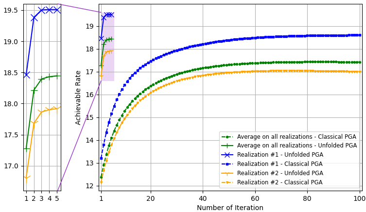
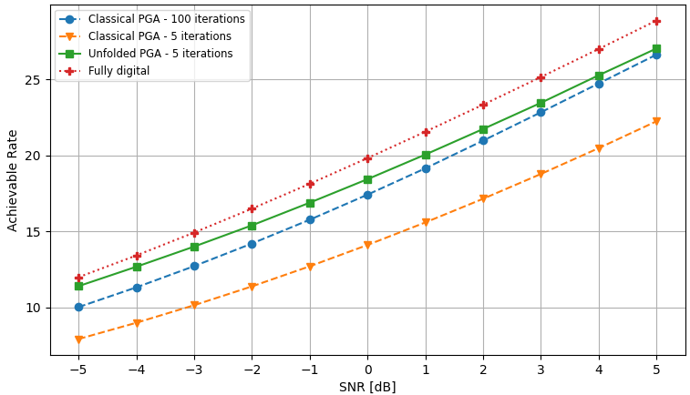
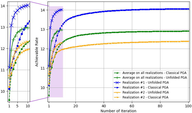
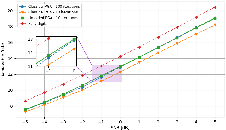
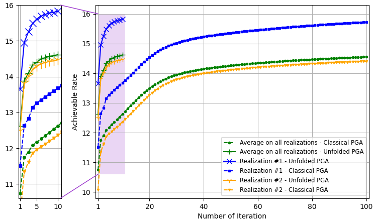
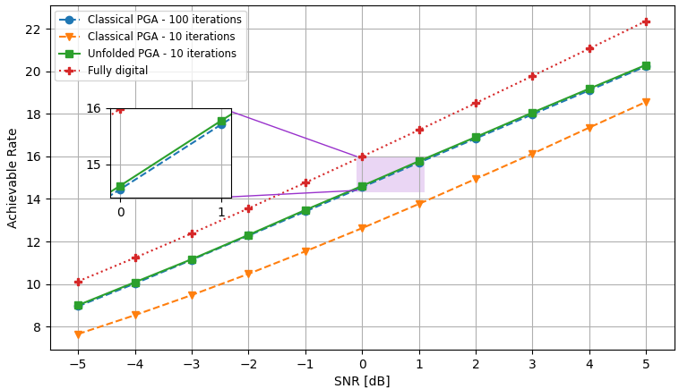
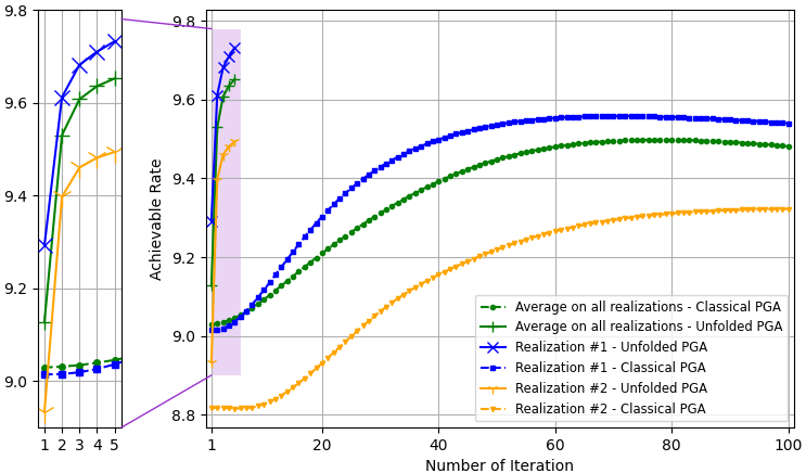
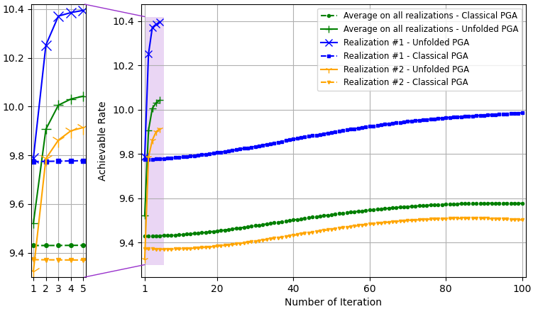
The PGA hybrid precoding design with optimized iterations is compared with applying PGA with fixed hyperparameters, where we used a constant step size chosen based on empirical trials. Both hybrid precoders are evaluated over unseen test channels. The simulation results for the settings of , , and are depicted in Fig. 3, Fig. 4, and Fig. 5, respectively, where each figure compares both the convergence of the algorithms averaged over all channel realizations and for the randomly chose realizations, as well as the resulting sum-rates versus SNR.
The resulting sum-rates (for SNRdB) versus the number of PGA iterations, of both the unfolded PGA and the classical PGA (with manually chosen constant step sizes), when averaged over all unseen channels, and for two random channel realizations, are depicted in Fig. 3(a), Fig. 4(a), and Fig. 5(a). We observe in these figures that the proposed learn-to-optimize consistently facilitates simple PGA optimization of the hybrid precoders, achieving similar and even surpassing the sum-rates achieved by conventional PGA with fixed step sizes, while requiring much fewer iterations. The reduction in the number of iterations due to learn-to-optimize is by factors of ( iterations vs. iterations) and ( iterations vs. iterations) in speed, compared to conventional fixed-size optimization. These gains are consistent over the different channel models and configurations considered. Fig. 3(b), Fig. 4(b), and Fig. 5(b) illustrate the sum-rate for different values of SNR, of the proposed unfolded PGA compared with that of the classical PGA and the sum-rate resulting from fully digital baseband precoding, serving as an upper bound on the achievable sum-rate. The figures show the gain of converting the classical PGA algorithm in a discriminative trainable model. In particular, the unfolded algorithm implements PGA with merely few iterations while systematically improving upon conventional PGA with fixed step size and iterations. These results demonstrate the benefits of the proposed approach in leveraging data to improve both performance and convergence speed while preserving the interpretability and suitability of conventional iterative optimizers.
V-A2 PGA using phase shifters networks
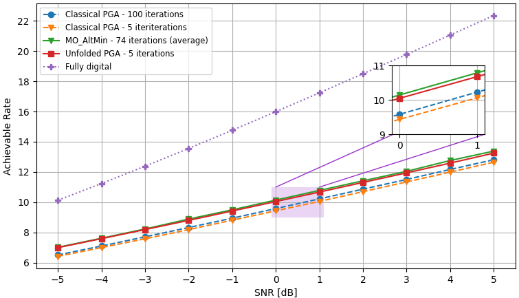
The numerical evaluation above showed that the considered deep unfolding methodology indeed facilitates rapid optimization of hybrid precoders. To demonstrate that these gains are not unique to unconstrained analog combiners, as well as to compare with alternative iterative optimizers, we next consider phase shifters networks for the implementation of the analog architecture, as often considered in the literature. This means that the projection in (11) is used in Step 1 of Algorithm 1. We used as a benchmark the MO-AltMin algorithm of [15], which is designed to iteratively optimize such constrained hybrid precoders.
We consider the QuaDRiGa channel model for two different settings of the number frequency bands , users , RF chains , and transmit antennas: ; and . Similarly to the unconstrained case, for each setting, we apply Algorithm 2 to learn the hyperparameters for which the PGA converges with iterations. In the training procedure we use channels for each setting, where we used epochs with batch size and used Adam for the update in Step 2. The PGA with learned iterations is compared with the PGA with fixed hyperparameters, chosen empirically. The hybrid precoders optimizers are evaluated over unseen test channels. The performance evaluation results are shown in Fig. 6, and Fig. 7, for the settings of , and , respectively, where each figure examines both the convergence curves as well as the sum-rate achieved at the end of the optimization procedure versus SNR.
The resulting sum-rate (for SNRdB) versus the number of PGA iterations, when averaged over all unseen channels, and of two random channel realizations, is shown in Fig. 6(a), and Fig. 7(a). We observe in these figures that the learn-to-optimize method is able to accelerate and outperform the PGA optimization, when compared to the standard PGA, with constant, manually chosen, step sizes. Observe that the number of iterations is reduced by ( iterations vs. ), compared to standard optimization. The gain in performance systematically observed here follows from the ability of data-driven optimization to facilitate coping with the non-convex nature of the resulting optimization problem. Fig. 6(b), and Fig. 7(b) demonstrate the comparison between the proposed unfolded PGA, the classical PGA, the MO-Altmin algorithm of [15], and fully digital baseband precoding. It is shown that the gap from the fully digital baseband precoding is significant, due to the use of a relatively small number of RF chains in the hybrid architecture. When comparing the iterative algorithms we see a small difference in terms of sum-rate, but it is important to consider the fact that the proposed unfolded PGA operates with the least number of iterations, therefor it achieves improvement in terms of speed when comparing to the benchmark and to the standard PGA. These results show the ability of the proposed learn-to-optimize technique to tackle and incorporate different constraints into the PGA algorithm while enabling rapid performance and fully preserving interpretability.

V-B Hybrid Precoding with Noisy CSI
The numerical studies reported in Subsection V-A empirically validate the ability of the proposed methodology to facilitate rapid optimization under different settings. We next demonstrate its ability to simultaneously enable rapid and robust hybrid precoding. Hence, in the following, we consider the unfolding of the PCMP algorithm for precoding under noisy channel estimation. Having demonstrated the ability of our approach to deal with constrained precoders, we focus here on unconstrained analog combiners. According, we implement of the learn-to-optimize methodology, i.e. Algorithm 4, for Algorithm 3, when the projection operator applied on the analog precoder in Step 3 is set to be . The set of considered error patterns is comprised of patterns randomly generated with Frobenius norm values in the range , and we evaluate the maximin rate over .
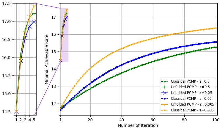
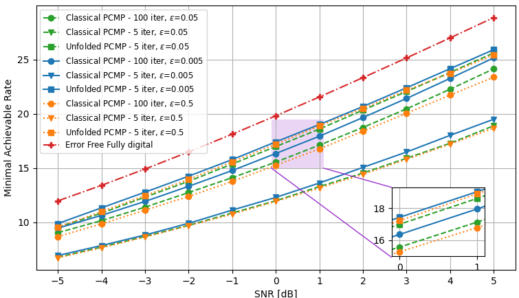
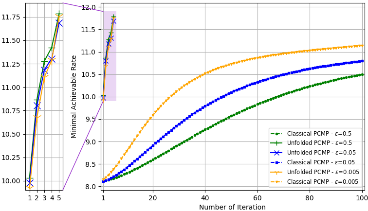
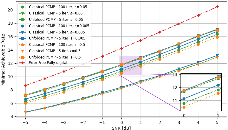
We examine two different settings of the number frequency bands , users , RF chains , transmit antennas , and the data source: , with Rayleigh channels; and with QuaDRiGa channel model, the simulations results for each setting are demonstrated in Fig. 8, and Fig. 9, respectively. Again, we evaluate both the convergence rate and the minimal rate (within the tolerable error regime) at the end of the optimization procedure versus SNR, and compare our results with the conventional PCMP optimizer. In the simulations, three error bound values are considered, . For each setting, we applied Algorithm 4 to learn to set hybrid precoders with iterations based on channels, where we used epochs with batch size , and used Adam for the update in Step 4. We compared the standard PCMP, with constant hyperparameters, to the optimized PCMP with exactly iterations.
Fig. 8(a) and Fig. 9(a) depict the minimal sum-rates, averaged on unseen test channels results, for the three error bound values, vs. the number of PCMP iterations. In these figures, we observe notable gains in convergence speed of a factor of ( iterations vs. iterations), and it is shown that the performances of the learned PCMP algorithm consistently surpasses the performances of the conventional PCMP with constant step sizes. In Fig. 8(b), and Fig. 9(b), the sum-rate for different values of SNR is shown. These figures include the fully digital baseband precoding error-free sum-rates, which are calculated with full CSI, and reflect on the best performance one can achieve given full CSI and without RF chain reduction. We observe that the proposed robust optimization method, the unfolded PCMP, achieves relatively close performances to the full-CSI fully digital baseband precoding, systematically outperforming the model-based PCMP operating with much more iterations. These results demonstrates the gains and advantages of our proposed learn-to-optimize method in enabling optimization of hybrid precoders which is both rapid and robust.
VI Conclusions
In this work we proposed a method to leverage data to enable rapid, robust, and interpretable tuning of hybrid precoders. Our approach unfolds a suitable optimizer for maximizing the minimal sum-rate within a given tolerable CSI error into a fixed and small number of iterations. Then, we use data to tune the hyperparameters of each iteration. Our method is shown to notably improve convergence speed while setting hybrid precoders which achieve similar and even improved sum-rates compared to those tuned via lengthy non-learned optimization.
VII Acknowledgements
The authors would like to thank Tomer Yeblonka from CEVA for his valuable inputs and meaningful discussions.
Appendix A Complex Gradients of with Respect to
Appendix B Complex Gradient of with Respect to
The complex differential of with respect to is given by
References
- [1] O. Agiv and N. Shlezinger, “Learn to rapidly optimize hybrid precoding,” in Proc. IEEE SPAWC, 2022.
- [2] “6G - the next hyper connected experience for all,” Samsung, 2020.
- [3] T. L. Marzetta, “Noncooperative cellular wireless with unlimited numbers of base station antennas,” IEEE Trans. Wireless Commun., vol. 9, no. 11, p. 3590, 2010.
- [4] E. Björnson, J. Hoydis, and L. Sanguinetti, “Massive MIMO networks: Spectral, energy, and hardware efficiency,” Foundations and Trends® in Signal Processing, vol. 11, no. 3-4, pp. 154–655, 2017.
- [5] N. Shlezinger and Y. C. Eldar, “On the spectral efficiency of noncooperative uplink massive MIMO systems,” IEEE Trans. Commun., vol. 67, no. 3, pp. 1956–1971, 2019.
- [6] X. Gao, L. Dai, and A. M. Sayeed, “Low RF-complexity technologies to enable millimeter-wave MIMO with large antenna array for 5G wireless communications,” IEEE Commun. Mag., vol. 56, no. 4, pp. 211–217, 2018.
- [7] A. F. Molisch, V. V. Ratnam, S. Han, Z. Li, S. L. H. Nguyen, L. Li, and K. Haneda, “Hybrid beamforming for massive MIMO: A survey,” IEEE Commun. Mag., vol. 55, no. 9, pp. 134–141, 2017.
- [8] I. Ahmed, H. Khammari, A. Shahid, A. Musa, K. S. Kim, E. De Poorter, and I. Moerman, “A survey on hybrid beamforming techniques in 5G: Architecture and system model perspectives,” IEEE Commun. Surveys Tuts., vol. 20, no. 4, pp. 3060–3097, 2018.
- [9] R. Méndez-Rial, C. Rusu, N. González-Prelcic, A. Alkhateeb, and R. W. Heath, “Hybrid MIMO architectures for millimeter wave communications: Phase shifters or switches?” IEEE Access, vol. 4, pp. 247–267, 2016.
- [10] S. S. Ioushua and Y. C. Eldar, “A family of hybrid analog–digital beamforming methods for massive MIMO systems,” IEEE Trans. Signal Process., vol. 67, no. 12, pp. 3243–3257, 2019.
- [11] T. Gong, N. Shlezinger, S. S. Ioushua, M. Namer, Z. Yang, and Y. C. Eldar, “RF chain reduction for MIMO systems: A hardware prototype,” IEEE Syst. J., vol. 14, no. 4, pp. 5296–5307, 2020.
- [12] T. Zirtiloglu, N. Shlezinger, Y. C. Eldar, and R. T. Yazicigil, “Power-efficient hybrid MIMO reciever with task-specific beamforming using low-resolution ADCs,” in Proc. IEEE ICASSP, 2022, pp. 5338–5342.
- [13] S. Park, A. Alkhateeb, and R. W. Heath, “Dynamic subarrays for hybrid precoding in wideband mmWave MIMO systems,” IEEE Trans. Wireless Commun., vol. 16, no. 5, pp. 2907–2920, 2017.
- [14] M. A. Albreem, A. H. Al Habbash, A. M. Abu-Hudrouss, and S. S. Ikki, “Overview of precoding techniques for massive MIMO,” IEEE Access, vol. 9, pp. 60 764–60 801, 2021.
- [15] X. Yu, J.-C. Shen, J. Zhang, and K. B. Letaief, “Alternating minimization algorithms for hybrid precoding in millimeter wave MIMO systems,” IEEE J. Sel. Topics Signal Process., vol. 10, no. 3, pp. 485–500, 2016.
- [16] F. Sohrabi and W. Yu, “Hybrid digital and analog beamforming design for large-scale antenna arrays,” IEEE J. Sel. Topics Signal Process., vol. 10, no. 3, 2016.
- [17] N. Shlezinger, G. C. Alexandropoulos, M. F. Imani, Y. C. Eldar, and D. R. Smith, “Dynamic metasurface antennas for 6G extreme massive MIMO communications,” IEEE Commun. Mag., vol. 28, no. 2, pp. 106–113, 2021.
- [18] H. Zhang, N. Shlezinger, F. Guidi, D. Dardari, M. F. Imani, and Y. C. Eldar, “Beam focusing for near-field multi-user MIMO communications,” IEEE Trans. Wireless Commun., vol. 21, no. 9, pp. 7476–7490, 2022.
- [19] A. Zappone, M. Di Renzo, and M. Debbah, “Wireless networks design in the era of deep learning: Model-based, AI-based, or both?” IEEE Trans. Commun., vol. 67, no. 10, pp. 7331–7376, 2019.
- [20] T. Chen, X. Chen, W. Chen, H. Heaton, J. Liu, Z. Wang, and W. Yin, “Learning to optimize: A primer and a benchmark,” arXiv preprint arXiv:2103.12828, 2021.
- [21] Q. Hu, Y. Cai, K. Kang, G. Yu, J. Hoydis, and Y. C. Eldar, “Two-timescale end-to-end learning for channel acquisition and hybrid precoding,” IEEE J. Sel. Topics Signal Process., vol. 40, no. 1, pp. 163–181, 2021.
- [22] H. Huang, Y. Song, J. Yang, G. Gui, and F. Adachi, “Deep-learning-based millimeter-wave massive MIMO for hybrid precoding,” IEEE Trans. Veh. Technol., vol. 68, no. 3, pp. 3027–3032, 2019.
- [23] H. Huang, Y. Peng, J. Yang, W. Xia, and G. Gui, “Fast beamforming design via deep learning,” IEEE Trans. Veh. Technol., vol. 69, no. 1, pp. 1065–1069, 2019.
- [24] A. M. Elbir and A. K. Papazafeiropoulos, “Hybrid precoding for multiuser millimeter wave massive MIMO systems: A deep learning approach,” IEEE Trans. Veh. Technol., vol. 69, no. 1, pp. 552–563, 2019.
- [25] A. M. Elbir, K. V. Mishra, and S. Chatzinotas, “Terahertz-band joint ultra-massive MIMO radar-communications: Model-based and model-free hybrid beamforming,” IEEE J. Sel. Topics Signal Process., vol. 15, no. 6, pp. 1468–1483, 2021.
- [26] T. Peken, S. Adiga, R. Tandon, and T. Bose, “Deep learning for SVD and hybrid beamforming,” IEEE Trans. Wireless Commun., vol. 19, no. 10, pp. 6621–6642, 2020.
- [27] H. Hojatian, J. Nadal, J.-F. Frigon, and F. Leduc-Primeau, “Unsupervised deep learning for massive MIMO hybrid beamforming,” IEEE Trans. Wireless Commun., vol. 20, no. 11, pp. 7086–7099, 2021.
- [28] Q. Hu, Y. Liu, Y. Cai, G. Yu, and Z. Ding, “Joint deep reinforcement learning and unfolding: Beam selection and precoding for mmWave multiuser MIMO with lens arrays,” IEEE J. Sel. Areas Commun., vol. 39, no. 8, pp. 2289–2304, 2021.
- [29] Q. Wang, K. Feng, X. Li, and S. Jin, “PrecoderNet: Hybrid beamforming for millimeter wave systems with deep reinforcement learning,” IEEE Commun. Lett., vol. 9, no. 10, pp. 1677–1681, 2020.
- [30] N. Shlezinger, J. Whang, Y. C. Eldar, and A. G. Dimakis, “Model-based deep learning,” arXiv preprint arXiv:2012.08405, 2020.
- [31] N. Shlezinger, Y. C. Eldar, and S. P. Boyd, “Model-based deep learning: On the intersection of deep learning and optimization,” IEEE Access, vol. 10, pp. 115 384–115 398, 2022.
- [32] A. Balatsoukas-Stimming and C. Studer, “Deep unfolding for communications systems: A survey and some new directions,” in Proc. IEEE SiPS, 2019, pp. 266–271.
- [33] A. Balatsoukas-Stimming, O. Castañeda, S. Jacobsson, G. Durisi, and C. Studer, “Neural-network optimized 1-bit precoding for massive MU-MIMO,” in Proc. IEEE SPAWC, 2019.
- [34] L. Pellaco, M. Bengtsson, and J. Jaldén, “Matrix-inverse-free deep unfolding of the weighted MMSE beamforming algorithm,” IEEE Open Journal of the Communications Society, vol. 3, pp. 65–81, 2021.
- [35] J. Luo, J. Fan, and J. Zhang, “MDL-AltMin: A hybrid precoding scheme for mmWave systems with deep learning and alternate optimization,” IEEE Commun. Lett., vol. 11, no. 9, pp. 1925–1929, 2022.
- [36] S. Shi, Y. Cai, Q. Hu, B. Champagne, and L. Hanzo, “Deep-unfolding neural-network aided hybrid beamforming based on symbol-error probability minimization,” IEEE Trans. Veh. Technol., 2022, early access.
- [37] E. Balevi and J. G. Andrews, “Unfolded hybrid beamforming with GAN compressed ultra-low feedback overhead,” IEEE Trans. Wireless Commun., vol. 20, no. 12, pp. 8381–8392, 2021.
- [38] K.-Y. Chen, H.-Y. Chang, R. Y. Chang, and W.-H. Chung, “Hybrid beamforming in mmwave MIMO-OFDM systems via deep unfolding,” in Vehicular Technology Conference:(VTC2022-Spring). IEEE, 2022.
- [39] K. K. Thekumparampil, P. Jain, P. Netrapalli, and S. Oh, “Efficient algorithms for smooth minimax optimization,” Advances in Neural Information Processing Systems, vol. 32, 2019.
- [40] S. Jaeckel, L. Raschkowski, K. Börner, and L. Thiele, “Quadriga: A 3-D multi-cell channel model with time evolution for enabling virtual field trials,” IEEE Trans. Antennas Propag., vol. 62, no. 6, pp. 3242–3256, 2014.
- [41] X. Gao, L. Dai, S. Han, I. Chih-Lin, and R. W. Heath, “Energy-efficient hybrid analog and digital precoding for mmWave MIMO systems with large antenna arrays,” IEEE J. Sel. Areas Commun., vol. 34, no. 4, pp. 998–1009, 2016.
- [42] Z. Shen, R. Chen, J. G. Andrews, R. W. Heath, and B. L. Evans, “Sum capacity of multiuser MIMO broadcast channels with block diagonalization,” IEEE Trans. Wireless Commun., vol. 6, no. 6, pp. 2040–2045, 2007.
- [43] A. Goldsmith, Wireless communications. Cambridge, 2005.
- [44] S. Boyd and L. Vandenberghe, Convex optimization. Cambridge, 2004.
- [45] N. Shlezinger and T. Routtenberg, “Discriminative and generative learning for linear estimation of random signals [lecture notes],” arXiv preprint arXiv:2206.04432, 2022.
- [46] N. Samuel, T. Diskin, and A. Wiesel, “Learning to detect,” IEEE Trans. Signal Process., vol. 67, no. 10, pp. 2554–2564, 2019.
- [47] A. Mokhtari, A. Ozdaglar, and S. Pattathil, “A unified analysis of extra-gradient and optimistic gradient methods for saddle point problems: Proximal point approach,” in International Conference on Artificial Intelligence and Statistics. PMLR, 2020, pp. 1497–1507.
- [48] P. I. Frazier, “A tutorial on Bayesian optimization,” arXiv preprint arXiv:1807.02811, 2018.
- [49] A. Hjörungnes, Complex-valued matrix derivatives with applications in signal processing and communications. Cambridge, 2011.