Learning Debiased Classifier with Biased Committee

Nayeong Kim Sehyun Hwang Sungsoo Ahn Jaesik Park Suha Kwak
Pohang University of Science and Technology (POSTECH), South Korea
{nayeong.kim, sehyun03, sungsoo.ahn, jaesik.park, suha.kwak}@postech.ac.kr

Abstract

Neural networks are prone to be biased towards spurious correlations between classes and latent attributes exhibited in a major portion of training data, which ruins their generalization capability. We propose a new method for training debiased classifiers with no spurious attribute label. The key idea is to employ a committee of classifiers as an auxiliary module that identifies bias-conflicting data, i.e., data without spurious correlation, and assigns large weights to them when training the main classifier. The committee is learned as a bootstrapped ensemble so that a majority of its classifiers are biased as well as being diverse, and intentionally fail to predict classes of bias-conflicting data accordingly. The consensus within the committee on prediction difficulty thus provides a reliable cue for identifying and weighting bias-conflicting data. Moreover, the committee is also trained with knowledge transferred from the main classifier so that it gradually becomes debiased along with the main classifier and emphasizes more difficult data as training progresses. On five real-world datasets, our method outperforms prior arts using no spurious attribute label like ours and even surpasses those relying on bias labels occasionally. Our code is available at https://github.com/nayeong-v-kim/LWBC.

1 Introduction

Most supervised learning algorithms for classification rely on the empirical risk minimization (ERM) principle [41]. However, ERM has been known to cause a learned classifier to be biased toward spurious correlations between predefined classes and latent attributes that appear in a majority of training data [12]. In the case of hair color classification, for example, when most people with blond-hair (i.e., target class) are female (i.e., latent attribute) in a dataset, a classifier learned by ERM exploits female as a shortcut for the classification due to its spurious correlation with blond-hair, and often mis-classifies non-blonde-haired women as blond-hair in consequence. We call data with such spurious correlations and holding a majority of training data bias-guiding samples, and the other bias-conflicting samples, respectively. The issue of model bias has often been addressed by exploiting explicit spurious attribute labels [22, 29, 37, 2, 40, 39, 46] or knowledge about bias types given a priori [3]. However, these methods are impractical because such supervision and prior knowledge are costly, and the methods demand extensive post hoc analysis.

Hence, a body of research has been conducted for learning debiased classifiers with no additional label for spurious attributes [43, 28, 30, 33, 23, 27]. A common approach in this line of work is to employ an intentionally biased classifier as an auxiliary module [30, 33, 23, 27]. In this approach, samples that the biased classifier has trouble handling are regarded as bias-conflicting ones and assigned large weights when used for training the main classifier to reduce the effect of bias-guiding counterparts. Although it has driven remarkable success, this approach has drawbacks due to the use of a single biased classifier. First, the quality of the biased classifier could vary by hyper-parameters [30] and its initial parameter values [11]. Further, data that the biased classifier fails to handle could include not only bias-conflicting samples but also bias-guiding ones, which differs by the quality of the classifier. These drawbacks limit the reliability and performance of debiasing methods depending on a single biased classifier, as demonstrated in Figure 1.

To overcome these limitations, we propose a new method using a committee of biased classifiers as the auxiliary module, coined learning with biased committee (LWBC). LWBC identifies bias-conflicting samples and determines their weights through consensus on their prediction difficulty within the committee. To this end, the committee is built as a bootstrapped ensemble, i.e., each of its classifiers is trained from a randomly sampled subset of the entire training dataset. This strategy not only guarantees the diversity among the classifiers, but also lets a majority of the classifiers be biased since random subsets of training data are highly likely to be dominated by bias-guiding samples. Accordingly, a majority of the committee tends to classify bias-guiding samples correctly and fail to deal with bias-conflicting ones. The consensus on prediction difficulty within the committee thus gives a strong cue for identifying and weighting bias-conflicting samples. Also, using the consensus of multiple classifiers enables LWBC to be robust to the varying quality of individual classifiers and consequently to focus more precisely on bias-conflicting samples, as shown in Figure 1.

Moreover, unlike the biased classifier trained independently of the main classifier in the previous work, the committee in LWBC is trained with knowledge of the main classifier as well as the random subsets of training data to serve the main classifier better. Specifically, the knowledge is distilled in the form of classification logits of the main classifier [18], and each classifier of the committee utilizes the knowledge as pseudo labels of training data other than its own training set. We expect that this strategy allows the committee to become debiased gradually so that it does not give large weights to easy bias-conflicting samples, i.e., those already well handled by the main classifier, and focuses more on difficult ones. Note that, even with this strategy, the classifiers of the committee are still biased differently due to their different training sets with ground-truth labels.

Finally, we further improve the proposed method by adopting a self-supervised representation as the frozen backbone of the committee and the main classifier. Since self-supervised learning is not dependent on class labels, it is less affected by the spurious correlations between classes and latent attributes, leading to a robust and less-biased representation. Also, by installing the committee and the main classifier on top of the representation, the classifiers can be implemented efficiently in both space and time while enjoying the rich and bias-free features given by the backbone.

LWBC is validated extensively on five real-world datasets. It substantially outperforms existing methods using no bias label and even occasionally surpasses previous arts demanding bias labels. We also demonstrate that all of the main components, i.e., the use of the committee, its training with knowledge transfer, and the self-supervised learning, contribute to the outstanding performance. The main contribution of this paper is four-fold:

•

We present LWBC, a new approach to learning a debiased classifier with no spurious attribute label. The use of consensus within the committee allows LWBC to address limitations of previous work relying on a single biased classifier.
•

We propose to learn the committee using knowledge of the main classifier, unlike the previous work whose auxiliary modules do not consider the main classifier.
•

We investigate the potential of self-supervised learning for debiasing, and find that it is a solid yet unexplored baseline for the task.
•

LWBC demonstrates superior performance on five real-world datasets. It outperforms existing methods using no additional supervision like ours and even surpasses those relying on spurious attribute labels occasionally.

2 Related work

2.1 Debiasing with prior knowledge on bias

A majority of previous work on learning debiased classifiers mitigates the bias by leveraging explicit labels on bias types [22, 29, 37, 2, 40, 39, 46]. For instance, Kim et al. [22] build a debiased model to classify digits by leveraging RGB color labels explicitly in the Colored MNIST dataset. Other methods are designed to handle predefined domain-specific bias types (e.g., texture bias in ImageNet) [42, 5, 3].

Recent methods try to reduce annotation costs for bias supervision by only utilizing a small set of bias-labeled data. For instance, Nam et al. [34] and Jung et al. [21] train auxiliary bias predictor with a small set of bias-labeled data and assign pseudo bias labels to the entire training set using its prediction. These methods have two inherent limitations. First, they cannot handle biases whose types are not predefined in training. Second, manually annotating all bias types is often expensive and laborious. Even obtaining a small set of bias labels could be expensive since bias labels existing in a real-world dataset is often long-tailed [31] or multi-labeled [16].

2.2 Debiasing without spurious attribute labels

Recent debiasing methods without any bias supervision [19, 8, 33, 27, 23, 30, 7, 1, 38, 26, 35] are based on the assumption that attributes of malignant bias are easier to learn than those of target classes. Through this assumption, previous methods identify the amount of biases within the samples and train a robust models by emphasizing bias-conflicting samples. To identify biases of samples, previous work leverage a high gradient of the latent vector [19, 8] or employ an intentionally biased classifier as an auxiliary module [33, 23, 27] by using generalized cross-entropy (GCE) loss [45]. Liu et al. [30] consider misclassified samples as bias-conflicting samples, and Creager et al. [7] derive bias-guiding and bias-conflicting partition that maximally violates the invariance principle. On the other hand, Bahng et al. [3] propose a method tailored to the texture bias, building a debiased model to learn independent features from a biased model in which receptive field size is limited to capture the texture bias in image classification.

While LWBC is also based on the aforementioned assumption, we firstly propose to identify bias-conflicting samples and up-weight them through the consensus of a committee of the biased classifiers. By exploiting the consensus of multiple classifiers, LWBC is robust against the varying quality of individual classifiers and allows to learn debiased classifiers more reliably and effectively.

3 Proposed method

We propose a new method that learns a debiased classifier with a committee of biased classifiers, dubbed LWBC. It first learns a feature representation with self supervision, which is used as the frozen backbone providing rich and bias-free features to downstream modules (Section 3.1). Next, it trains a committee of $m$ auxiliary classifiers $f_{1},f_{2},\ldots,f_{m}$ and the main classifier $g$ on top of the self-supervised representation (Section 3.2); thanks to the self-supervised representation, the classifiers are designed concisely, using only two fully-connected layers for each.

In a nutshell, the committee identifies bias-conflicting samples and assigns them large weights to reduce the effect of bias-guiding samples during the training of the main classifier. To this end, the committee is trained as a bootstrapped ensemble of classifiers so that a majority of its classifiers are biased as well as diverse, and intentionally fail to predict classes of bias-conflicting samples accordingly. Hence, the consensus within the committee on prediction difficulty of a sample (e.g., the number of classifiers that fail to predict its class label) indicates how much likely the sample is bias-conflicting, and is used to compute weights for training samples. Moreover, the committee is trained also with knowledge of the main classifier so that it gradually becomes debiased along with the main classifier and emphasizes more difficult samples as training progresses. Note that the committee is an auxiliary module used only in training and thus does not impose additional computation or memory footprint in testing.

The overall process of LWBC is illustrated conceptually in Figure 2 and given formally in Algorithm 1. The following sections elaborate on each step of LWBC.

3.1 Self-supervised representation learning

As the feature extractor, we train a backbone network by self-supervised learning with BYOL [14] on the target dataset. During the self-supervised learning, a random patch of input image is cropped, resized to 224 $\times$ 224 pixels, flipped horizontally at random, and distorted by a random sequence of brightness, contrast, saturation, hue adjustments, and grayscale conversion.

A self-supervised model can capture diverse patterns shared by data without being biased towards a particular class even the training set is biased. We empirically demonstrate that adopting a self-supervised representation leads to a model less biased compared with a supervised representation.

Although the representation offers rich and less-biased features, the main classifier can be still biased when it is trained by ERM. In other words, the self-supervised representation alone is not enough to learn a debiased model, and the need to explore a debiasing method for a classifier arises. Hence, we propose LWBC, a new debiasing method illustrated in the next section.

3.2 Learning a debiased classifier with a biased committee

Algorithm 1 Learning a debiased classifier with a biased committee

0: training set

\mathcal{D}

, batch size

b

, size of the committee

m

, learning rate

\eta

, scale hyper-parameter

\alpha

, balancing hyper-parameter

\lambda

, total number of iterations

t

, number of warm-up iterations

t_{w}

1: Draw

m

random subsets

\mathcal{S}_{1},...,\mathcal{S}_{m}

\mathcal{D}

2: Initialize auxiliary classifiers of the committee

\{f_{l}(x;\theta_{l})\}_{l=1}^{m}

3: Initialize the main classifier

g(x;\phi)

4: for

j=1,...,t_{w}

5: Draw a mini-batch

\mathcal{B}=\{(x_{i},y_{i})\}_{i=1}^{b}

from

\mathcal{D}

\theta_{l}\leftarrow\theta_{l}-\eta\nabla_{\theta_{l}}\mathcal{L}_{\textrm{CE}}\;\;\forall l={1,...,m}

Eq. (1)

7: end for

8: for

j=t_{w}+1,...,t

9: Draw a mini-batch

\mathcal{B}=\{(x_{i},y_{i}))\}_{i=1}^{b}

from

\mathcal{D}

10:

w(x_{i})={1/(\sum_{l=1}^{m}\mathbbm{1}(f_{l}(x_{i})=y_{i})/m+\alpha)}\;\;\forall x_{i}\in\mathcal{B}

Eq. (2)

11:

\phi\leftarrow\phi-\eta\nabla_{\phi}\mathcal{L}_{\textrm{WCE}}

Eq. (3)

12:

\theta_{l}\leftarrow\theta_{l}-(1-\lambda)\eta\nabla_{\theta_{l}}\mathcal{L}_{\textrm{CE}}-\lambda\eta\nabla_{\theta_{l}}\mathcal{L}_{\textrm{KD}}\;\;\forall l={1,...,m}

Eq. (1), Eq. (4)

13: end for

First, we randomly sample $m$ subsets of the same size, denoted by $\mathcal{S}_{1},...,\mathcal{S}_{m}$ , from the entire training dataset $\mathcal{D}$ with replacement. Then $m$ auxiliary classifiers $f_{1},...,f_{m}$ of the committee are initialized randomly, and each of the subsets $\mathcal{S}_{l}$ is assigned to each auxiliary classifier $f_{l}$ as its training data.

The first step of LWBC is warm-up training of the committee; this is required to ensure that the committee is capable of identifying and weighting bias-conflicting samples at the beginning of the main training process. Given a mini-batch $\mathcal{B}$ at each warm-up iteration, the committee is trained by minimizing the cross-entropy loss below:

\mathcal{L}_{\textrm{CE}}=\sum_{l=1}^{m}\sum_{(x,y)\in{\mathcal{S}_{l}\cap\mathcal{B}}}\textrm{CE}(f_{l}(x),y).

(1)

Since each subset is sampled from the training set dominated by bias-guiding samples, a majority of auxiliary classifiers are also biased. At the same time, the classifiers are diverse due to their difference in initialization and training data.

After the warm-up stage, the main classifier and the committee are trained while interacting with each other. First, the main classifier is trained by the weighted cross entropy loss with the entire training set, where the sample weights are computed by considering consensus within the committee on prediction difficulty of the samples. Since a majority of auxiliary classifiers have trouble to handle bias-conflicting samples, we identify and weight bias-conflicting samples based on the number of auxiliary classifiers whose predictions are correct for the samples. The weight function $w$ is given by

w(x)=\frac{1}{\sum_{l=1}^{m}\mathbbm{1}(f_{l}(x)=y)/m+\alpha},

(2)

where $m$ is the size of the committee, $f_{l}$ means the $l$ -th classifier of the committee, and $\alpha$ is a scale hyper-parameter. The weight reflects how much the sample $x$ is likely to be bias-conflicting and decreases rapidly when the number of correctly predicting classifiers increases. Then we train the main classifier $g$ with emphasis on the bias-conflicting samples through the weight function $w$ . The weighted cross entropy loss $\mathcal{L}_{\textrm{WCE}}$ is given by

\mathcal{L}_{\textrm{WCE}}=\sum_{(x,y)\in\mathcal{B}}w(x)\cdot\textrm{CE}(g(x),y),

(3)

where $\mathcal{B}$ is the mini-batch.

During training, as the main classifier is gradually debiased, samples useful for debiasing the main classifier change accordingly. To focus more on bias-conflicting samples difficult for the main classifier, we inform the quality of the main classifier to the committee by distilling the knowledge of the main classifier in the form of its classification logits [18] and transferring the knowledge by minimizing the following KD loss:

\mathcal{L}_{\textrm{KD}}=\sum_{l=1}^{m}\sum_{(x,y)\in\mathcal{B}\setminus\mathcal{S}_{l}}\textrm{KL}\left(\textrm{softmax}\left(\frac{g(x)}{\tau}\right),\textrm{softmax}\left(\frac{f_{l}(x)}{\tau}\right)\right),

(4)

where $\tau$ is a temperature parameter. Note that we apply $\mathcal{L}_{\textrm{KD}}$ to the complement set of $\mathcal{S}_{l}$ to avoid auxiliary classifiers in the committee being identical to each other. By interacting with the main classifier, the committee gradually becomes debiased along with the main classifier. Hence, samples correctly predicted by the main classifier are less weighted and those with incorrect predictions are more weighted by the committee.

After the warm-up training, the main classifier and the auxiliary classifiers are alternately updated with a given mini-batch at each iteration. First, we forward every sample in a mini-batch to each auxiliary classifier and then compute weights of the samples using predictions of the auxiliary classifiers (Eq. (2)). With the weights, the main classifier is updated by Eq. (3) and the knowledge of the updated main classifier is transferred to the auxiliary classifiers by Eq. (4). Thus, the auxiliary classifiers are updated by minimizing both losses of Eq. (1) and Eq. (4):

\displaystyle\mathcal{L}_{\textrm{committee}}=(1-\lambda)\mathcal{L}_{\textrm{CE}}+\lambda\mathcal{L}_{\textrm{KD}},

(5)

where $\lambda$ is a balancing hyper-parameter.

Table 1: Guiding, Unbiased, and Conflicting metrics (%) for the CelebA dataset. For methods without spurious attribute labels, we mark the best and the second-best performance in bold and underline, respectively.

Method	Spurious attribute label	CelebA HairColor			CelebA HeavyMakeup
Method	Spurious attribute label	Guiding	Unbiased	Conflicting	Guiding	Unbiased	Conflicting
Group DRO [37]	✓	87.46 ${}_{\pm\text{0.00}}$	85.43 ${}_{\pm\text{0.53}}$	83.40 ${}_{\pm\text{0.67}}$	79.52 ${}_{\pm\text{0.00}}$	64.88 ${}_{\pm\text{0.42}}$	50.24 ${}_{\pm\text{0.68}}$
EnD [39]	✓	94.97 ${}_{\pm\text{0.00}}$	91.21 ${}_{\pm\text{0.22}}$	87.45 ${}_{\pm\text{1.06}}$	98.16 ${}_{\pm\text{0.00}}$	75.93 ${}_{\pm\text{1.31}}$	53.70 ${}_{\pm\text{5.24}}$
CSAD [46]	✓	91.19 ${}_{\pm\text{0.00}}$	89.36 ${}_{\pm\text{0.00}}$	87.53 ${}_{\pm\text{0.00}}$	82.32 ${}_{\pm\text{0.00}}$	67.88 ${}_{\pm\text{0.00}}$	53.44 ${}_{\pm\text{0.00}}$
ERM	✗	87.98 ${}_{\pm\text{0.00}}$	70.25 ${}_{\pm\text{0.35}}$	52.52 ${}_{\pm\text{0.19}}$	90.25 ${}_{\pm\text{0.00}}$	62.00 ${}_{\pm\text{0.02}}$	33.75 ${}_{\pm\text{0.28}}$
LfF [33]	✗	87.24 ${}_{\pm\text{0.00}}$	84.24 ${}_{\pm\text{0.37}}$	81.24 ${}_{\pm\text{1.38}}$	86.92 ${}_{\pm\text{0.00}}$	66.20 ${}_{\pm\text{1.21}}$	45.48 ${}_{\pm\text{4.43}}$
SSL+ERM	✗	94.15 ${}_{\pm\text{0.57}}$	80.48 ${}_{\pm\text{0.91}}$	66.79 ${}_{\pm\text{2.20}}$	93.00 ${}_{\pm\text{0.49}}$	66.30 ${}_{\pm\text{1.15}}$	39.50 ${}_{\pm\text{2.47}}$
LWBC	✗	90.57 ${}_{\pm\text{2.15}}$	88.90 ${}_{\pm\text{1.55}}$	87.22 ${}_{\pm\text{1.14}}$	86.42 ${}_{\pm\text{0.82}}$	70.29 ${}_{\pm\text{1.14}}$	51.28 ${}_{\pm\text{5.74}}$

Table 2: indistribution and Worst-group metrics (%) for the CelebA dataset. We also report the difference between indistribution and Worst-group as Gap. For methods without spurious attribute labels, we mark the best and the second-best performance in bold and underline, respectively.

Method	Backbone network	Spurious attribute label	CelebA HairColor
Method	Backbone network	Spurious attribute label	indistribution	Worst-group	Gap
Group DRO [37]	Resnet50	✓	93.1 ${}_{\pm\text{0.21}}$	88.5 ${}_{\pm\text{1.16}}$	04.6
SSA [34]	Resnet50	✓	92.8 ${}_{\pm\text{0.11}}$	89.8 ${}_{\pm\text{1.28}}$	03.0
ERM	Resnet50	✗	95.6 ${}_{\pm\text{0.00}}$	47.2 ${}_{\pm\text{0.00}}$	48.4
CVaR DRO [28]	Resnet50	✗	82.4 ${}_{\pm\text{0.00}}$	64.4 ${}_{\pm\text{0.00}}$	18.0
LfF [33]	Resnet50	✗	86.0 ${}_{\pm\text{0.00}}$	70.6 ${}_{\pm\text{0.00}}$	15.4
EIIL [7]	Resnet50	✗	91.9 ${}_{\pm\text{0.00}}$	83.3 ${}_{\pm\text{0.00}}$	08.6
JTT [30]	Resnet50	✗	88.0 ${}_{\pm\text{0.00}}$	81.1 ${}_{\pm\text{0.00}}$	06.9
SSL+ERM	Resnet18	✗	95.5 ${}_{\pm\text{0.0\phantom{0}}}$	38.5 ${}_{\pm\text{4.1\phantom{0}}}$	42.0
LWBC	Resnet18	✗	88.9 ${}_{\pm\text{1.7\phantom{0}}}$	85.5 ${}_{\pm\text{1.4\phantom{0}}}$	03.4

4 Experiments

4.1 Setup

Implementation details. We adopt ResNet-18 [15] as the self-supervised model and train it following the strategy of BYOL [14] on the target dataset. Since the color information is key feature for HairColor classification on the CelebA dataset, we vary only brightness and contrast for data augmentation of color distortion when training the model on CelebA. Since NICO and BAR are very small datasets, we initialize the self-supervised model with ImageNet [9] pretrained parameters; except for the experiments using BAR and NICO, the self-supervised model is trained from scratch. We use the self-supervised ResNet-18 as a backbone network except for the last fully connected layer. We set the batch size to {64, 64, 128, 256}, learning rate to {1e-3, 1e-3, 1e-4, 6e-3}, the size of the committee $m$ to {30, 30, 30, 40}, the size of subset $\mathcal{S}_{l}$ to {10, 10, 80, 300}, $\lambda$ to {0.9, 0.6, 0.6, 0.6}, and $\tau$ to {1, 1, 1, 2.5}, respectively for {BAR, NICO, Imagenet-9, CelebA}, and $\alpha$ to 0.02. Note that we run LWBC on 3 random seeds and report the average and the standard deviation.

Evaluation metrics. Six metrics are adopted for evaluation. Validation / Test: average accuracy on validation / test splits. Guiding: average accuracy on bias guiding samples per class. Conflicting: average accuracy on bias conflicting samples per class. Unbiased: average of Guiding and Conflicting per class. Worst-group: minimum average accuracy of group; we can group the validation and test samples by the target and the bias. Indistribution: weighted group average accuracy with weights corresponding to the relative propotion of each group in the training dataset.

Table 3: Validation, Unbiased, and Test metrics (%) evaluated on the ImageNet-9 and ImageNet-A datasets. For methods without spurious attribute labels, we mark the best and the second-best performance in bold and underline, respectively.

Method	Spurious attribute label	ImageNet-9		ImageNet-A
Method	Spurious attribute label	Validation	Unbiased	Test
StylisedIN [13]	✓	088.4 ${}_{\pm\text{0.5\phantom{0}}}$	086.6 ${}_{\pm\text{0.6\phantom{0}}}$	024.6 ${}_{\pm\text{1.4\phantom{0}}}$
LearnedMixin [6]	✓	064.1 ${}_{\pm\text{4.0\phantom{0}}}$	062.7 ${}_{\pm\text{3.1\phantom{0}}}$	015.0 ${}_{\pm\text{1.6\phantom{0}}}$
RUBi [5]	✓	090.5 ${}_{\pm\text{0.3\phantom{0}}}$	088.6 ${}_{\pm\text{0.4\phantom{0}}}$	027.7 ${}_{\pm\text{2.1\phantom{0}}}$
ERM	✗	090.8 ${}_{\pm\text{0.6\phantom{0}}}$	088.8 ${}_{\pm\text{0.6\phantom{0}}}$	024.9 ${}_{\pm\text{1.1\phantom{0}}}$
Biased (BagNet18) [4]	✗	067.7 ${}_{\pm\text{0.3\phantom{0}}}$	065.9 ${}_{\pm\text{0.3\phantom{0}}}$	018.8 ${}_{\pm\text{1.15}}$
ReBias [3]	✗	091.9 ${}_{\pm\text{1.7\phantom{0}}}$	090.5 ${}_{\pm\text{1.7\phantom{0}}}$	029.6 ${}_{\pm\text{1.6\phantom{0}}}$
LfF [33]	✗	086.0 ${}_{\pm\text{0.00}}$	085.0 ${}_{\pm\text{0.00}}$	024.6 ${}_{\pm\text{0.00}}$
CaaM [43]	✗	095.7 ${}_{\pm\text{0.00}}$	095.2 ${}_{\pm\text{0.00}}$	032.8 ${}_{\pm\text{0.00}}$
SSL+ERM	✗	94.18 ${}_{\pm\text{0.07}}$	93.18 ${}_{\pm\text{0.04}}$	34.21 ${}_{\pm\text{0.49}}$
LWBC	✗	94.03 ${}_{\pm\text{0.23}}$	93.04 ${}_{\pm\text{0.32}}$	35.97 ${}_{\pm\text{0.49}}$

4.2 Datasets

CelebA. CelebA [32] is a dataset for face recognition where each sample is labeled with 40 attributes. Following the experiment configuration suggested by Nam et al. [33], we focus on HairColor and HeavyMakeup attributes that are spuriously correlated with Gender attributes, i.e., most of the CelebA images with blond-hair are women. As a result, the biased model suffers from performance degradation when predicting HairColor attribute on males. Therefore, we use HairColor as the target attribute and Gender as a spurious attribute, the same as HeavyMakeup.

ImageNet-9. ImageNet-9 [20] is a subset of ImageNet [36] containing nine super-classes. Following the setting adopted by Bahng et al. [3], we conduct experiments with 54,600 training images and 2,100 validation images. ImageNet-9 has been known to have a correlations between object class and image texture. We follow the evaluation scheme adopted by Bahng et al. [3], and we report the unbiased accuracy of the validation set, which is computed as average accuracy on every object-texture combination.

ImageNet-A. ImageNet-A [17] contains real-world images misclassified by an ImageNet-trained ResNet 50 [15]. Since such failures are caused when the model too heavily relies on colors, textures, and backgrounds, ImageNet-A could be regarded as a bias-conflicting set w.r.t. various ImageNet biases. This dataset is used only for evaluating a model trained on ImageNet-9.

BAR. The Biased Action Recognition (BAR) dataset [33] is a real-world image dataset intentionally designed to exhibit spurious correlations between human action and place on its images. Originally the training set of BAR consists of only bias-guiding samples, and its test set consists of only bias-conflicting samples. In our setting, we use 10% of the original BAR training set as validation and set the bias-conflicting ratio of the training set to 1%.

NICO. NICO [16] is a real-world dataset for simulating out-of-distribution image classification scenarios. Following the setting used by Wang et al. [43], we use an animal subset of NICO, which is labeled with 10 object and 10 context classes for evaluating the debiasing methods. The training set consists of 7 context classes per object class and they are long-tailed distributed (e.g., dog images are more frequently coupled with the ‘on grass’ context than any of the other 6 contexts). The validation and test sets consist of 7 seen context classes and 3 unseen context classes per object class. We verify the ability of debiasing a model from object-context correlations through evaluation on NICO.

Table 4: Conflicting, Validation, and Test metrics (%) evaluated on the BAR dataset (a) and the NICO dataset (b). For methods without spurious attribute labels, we mark the best and the second-best performance in bold and underline, respectively.

Method	Spurious attribute label	BAR
Method	Spurious attribute label	Conflicting
ERM	✗	35.32 ${}_{\pm\text{0.46}}$
ReBias [3]	✗	37.02 ${}_{\pm\text{0.26}}$
LfF [33]	✗	48.15 ${}_{\pm\text{0.93}}$
LDD [27]	✗	52.31 ${}_{\pm\text{1.00}}$
SSL+ERM	✗	60.88 ${}_{\pm\text{0.80}}$
LWBC	✗	62.03 ${}_{\pm\text{0.74}}$

(a) BAR dataset

Method	Spurious attribute label	NICO
Method	Spurious attribute label	Validation	Test
Cutout [10]	✓	43.69 ${}_{\pm\text{0.00}}$	43.77 ${}_{\pm\text{0.00}}$
RUBi [5]	✓	43.86 ${}_{\pm\text{0.00}}$	44.37 ${}_{\pm\text{0.00}}$
IRM [2]	✓	40.62 ${}_{\pm\text{0.00}}$	41.46 ${}_{\pm\text{0.00}}$
Unshuffle [40]	✓	43.15 ${}_{\pm\text{0.00}}$	43.00 ${}_{\pm\text{0.00}}$
REx [25]	✓	41.00 ${}_{\pm\text{0.00}}$	41.15 ${}_{\pm\text{0.00}}$
ERM	✗	43.77 ${}_{\pm\text{0.00}}$	42.61 ${}_{\pm\text{0.00}}$
CBAM [44]	✗	42.15 ${}_{\pm\text{0.00}}$	42.46 ${}_{\pm\text{0.00}}$
ReBias [3]	✗	44.92 ${}_{\pm\text{0.00}}$	45.23 ${}_{\pm\text{0.00}}$
LfF [33]	✗	41.83 ${}_{\pm\text{0.00}}$	40.18 ${}_{\pm\text{0.00}}$
CaaM [43]	✗	46.38 ${}_{\pm\text{0.00}}$	46.62 ${}_{\pm\text{0.00}}$
SSL+ERM	✗	55.63 ${}_{\pm\text{0.54}}$	52.24 ${}_{\pm\text{0.27}}$
LWBC	✗	56.05 ${}_{\pm\text{0.45}}$	52.84 ${}_{\pm\text{0.31}}$

(b) NICO dataset

Table 5: Ablation studies using Worst-group metric (%) on the CelebA HairColor dataset. We study the impact of learning from a single biased classifier (row 2), learning by committee (row 3), and transferring the knowledge of the main classifier (row 4). We mark the best performance in bold.

Method					CelebA HairColor
SSL	ERM	Single	Committee	KD	Worst-group
✓	✓	✗	✗	✗	38.5 ${}_{\pm\text{4.1}}$
✓	✗	✓	✗	✗	64.1 ${}_{\pm\text{2.4}}$
✓	✗	✗	✓	✗	81.3 ${}_{\pm\text{2.3}}$
✓	✗	✗	✓	✓	85.5 ${}_{\pm\text{1.4}}$

4.3 Quantitative results

LWBC shows superior classification accuracy among the methods that do not use the spurious attribute label on the five real-world datasets. In Tables 1 & 2, we observe LWBC outperforms existing debiasing methods using no spurious attribute label and shows comparable Conflicting performance with methods that exploit spurious attribute labels on CelebA, which reflects gender bias in the real world. Especially, the gap between the indistribution accuracy of groups and worst-group accuracy of LWBC is much smaller than the other methods, suggesting that our model fairly predicts a sample that belongs to each group. Table 3 shows the results on ImageNet-9, which is dominated by texture bias, and ImageNet-A, which is regarded as a bias-conflicting set of ImageNet. LWBC is 9.7% better than CaaM [44] on the ImageNet-A dataset, i.e., LWBC is robust to texture bias and various ImageNet biases. Table 4(a) shows results on the BAR dataset. LWBC is 18.6% better than LDD, the previous state of the art. Compared with LfF [33] and LDD [27], which are debiasing methods with a single biased classifier, learning a debiased classifier with the biased committee is more effective. Table 4(b) shows the results on the NICO dataset. LWBC is 13.3% better than CaaM, which suggests that LWBC is better generalized to unseen spurious attributes. Note that the validation and test set of NICO have unseen context classes and are unbiased.

4.4 Ablation study

Self-supervised representation as a solid baseline. We empirically investigate the potential of self-supervised representation as a solid baseline for the debiasing task. We train a classifier on the top of the self-supervised representation by ERM. The results are denoted by ‘SSL+ERM’ and compared with ‘ERM’, which is a fully supervised classification model in Table 1, 2, 3, 4(a), 4(b). ‘SSL+ERM’ outperforms not only ERM but also the previous state-of-the-art on all the datasets except for CelebA. ‘SSL+ERM’ is less biased than the model trained by fully supervised learning.

Importance of each module in LWBC. Table 5 demonstrates through ablation studies [30, 33, 23, 27]: (1) learning from a single biased classifier, (2) learning with committee, and (3) transferring the knowledge of the main classifier. First, we train a classifier by ERM (row 1) then assign a weight value 50 to the wrongly predicted samples and 1 to other samples. Then re-training the classifier with the weights (row 2). Comparing these two results demonstrates that up-weighting scheme with a biased classifier is effective to debiasing a classifier. Then we increase the number of biased classifiers and compute the sample weights using our weight function Eq. (2) (row 3). Learning with the committee shows a remarkable improvement in the worst-group accuracy. Moreover, knowledge distillation that enables the committee to interact with the main classifier further improves performance (row 4).

Effectiveness of transferring knowledge of the main classifier. Figure 3a shows the range of unbiased validation accuracy of classifiers in the committee and unbiased validation accuracy of the main classifier during training. The mean accuracy of classifiers in the committee gradually increases following the accuracy of the main classifier. Also, the accuracy of the main classifier gradually increases as training progresses. On the other hand, the accuracy of classifiers in the committee trained without KD loss does not increase or even decrease.

Number of classifiers. We compare the results of the main classifier trained with the different number of auxiliary classifiers. Figure 3b shows the worst-group accuracy versus the number of auxiliary classifiers $m$ on CelebA. With a single auxiliary classifier, the main classifier shows the lowest worst-group accuracy, but the accuracy increases as $m$ increases. When larger than 40, the number of classifiers has little effect on learning the main classifier.

4.5 Qualitative results

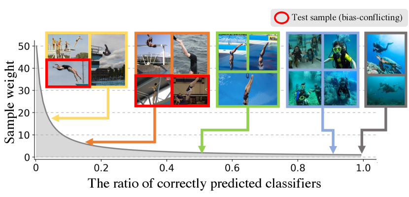
Figure 4 shows the graph of the weight function in Eq. (2) along with example images corresponding to specific weights. LWBC not only up-weights the bias-conflicting samples and down-weights the bias-guiding samples but also imposes fine-grained weights according to the difficulty of samples. For example, a majority of training samples of diving class on BAR are images of scuba diving or those of falling into the water with a blue background. In contrast, test samples of diving class are sport images of falling into water from a platform or springboard. As illustrated in Figure 4b, LWBC imposes fine-grained weights based on the proportion of the background in the image as well as down-weighting scuba diving images and up-weighting falling from platform images. The results demonstrate that LWBC more precisely distinguishes samples according to bias attributes.

5 Limitations

Self-supervised learning increases overall training complexity as it usually takes a longer time for convergence than supervised learning. Also, since the committee is designed as a bootstrapped ensemble, it involves randomness in training and thus causes noticeable performance fluctuation on CelebA, although it demonstrates stable performance on the other datasets.

6 Conclusion

We have proposed a new method for learning a debiased classifier with a committee of auxiliary classifiers. The committee is learned in a way that consensus on predictions of its classifiers offers a strong and reliable cue to identify and weight bias-conflicting data. The main debiased classifier is then trained with an emphasis on the bias-conflicting data to reduce the effect of bias-guiding counterparts. The committee is also trained to be debiased gradually along with the main classifier so that it highlights more challenging data as training progresses. Moreover, we demonstrated that self-supervised learning is a solid yet unexplored baseline for debiasing. Coupled with a self-supervised feature extractor, our method achieved state-of-the-art by large margins on most existing real-world datasets.

Acknowledgments and Disclosure of Funding

This work was supported by the NRF grants and the IITP grants funded by the Ministry of Education and the Ministry of Science and ICT, Korea (NRF-2021R1A2C3012728, 40%; NRF-2022R1A6A1A03052954, 20%; IITP-2022-0-00290, 30%; IITP-2019-0-01906, 10%).

References

[1] Faruk Ahmed, Yoshua Bengio, Harm van Seijen, and Aaron Courville. Systematic generalisation with group invariant predictions. In Proc. International Conference on Learning Representations (ICLR), 2021.
[2] Martin Arjovsky, Léon Bottou, Ishaan Gulrajani, and David Lopez-Paz. Invariant risk minimization. arXiv preprint arXiv:1907.02893, 2019.
[3] Hyojin Bahng, Sanghyuk Chun, Sangdoo Yun, Jaegul Choo, and Seong Joon Oh. Learning de-biased representations with biased representations. In Proc. International Conference on Machine Learning (ICML), pages 528–539. PMLR, 2020.
[4] Wieland Brendel and Matthias Bethge. Approximating cnns with bag-of-local-features models works surprisingly well on imagenet. arXiv preprint arXiv:1904.00760, 2019.
[5] Remi Cadene, Corentin Dancette, Matthieu Cord, Devi Parikh, et al. Rubi: Reducing unimodal biases for visual question answering. In Proc. Neural Information Processing Systems (NeurIPS), volume 32, pages 841–852, 2019.
[6] Christopher Clark, Mark Yatskar, and Luke Zettlemoyer. Don’t take the easy way out: Ensemble based methods for avoiding known dataset biases. In Proceedings of the 2019 Conference on Empirical Methods in Natural Language Processing and the 9th International Joint Conference on Natural Language Processing (EMNLP-IJCNLP), pages 4069–4082, 2019.
[7] Elliot Creager, Jörn-Henrik Jacobsen, and Richard Zemel. Environment inference for invariant learning. In International Conference on Machine Learning, pages 2189–2200. PMLR, 2021.
[8] Luke Darlow, Stanisław Jastrzębski, and Amos Storkey. Latent adversarial debiasing: Mitigating collider bias in deep neural networks. arXiv preprint arXiv:2011.11486, 2020.
[9] Jia Deng, Wei Dong, Richard Socher, Li-Jia Li, Kai Li, and Li Fei-Fei. ImageNet: a large-scale hierarchical image database. In Proc. IEEE Conference on Computer Vision and Pattern Recognition (CVPR), 2009.
[10] Terrance DeVries and Graham W Taylor. Improved regularization of convolutional neural networks with cutout. arXiv preprint arXiv:1708.04552, 2017.
[11] Stanislav Fort, Huiyi Hu, and Balaji Lakshminarayanan. Deep ensembles: A loss landscape perspective. arXiv preprint arXiv:1912.02757, 2019.
[12] Robert Geirhos, Jörn-Henrik Jacobsen, Claudio Michaelis, Richard Zemel, Wieland Brendel, Matthias Bethge, and Felix A Wichmann. Shortcut learning in deep neural networks. Nature Machine Intelligence, 2(11):665–673, 2020.
[13] Robert Geirhos, Patricia Rubisch, Claudio Michaelis, Matthias Bethge, Felix A. Wichmann, and Wieland Brendel. Imagenet-trained CNNs are biased towards texture; increasing shape bias improves accuracy and robustness. In Proc. International Conference on Learning Representations (ICLR), 2019.
[14] Jean-Bastien Grill, Florian Strub, Florent Altché, Corentin Tallec, Pierre H Richemond, Elena Buchatskaya, Carl Doersch, Bernardo Avila Pires, Zhaohan Daniel Guo, Mohammad Gheshlaghi Azar, et al. Bootstrap your own latent: A new approach to self-supervised learning. In Proc. Neural Information Processing Systems (NeurIPS), 2020.
[15] Kaiming He, Xiangyu Zhang, Shaoqing Ren, and Jian Sun. Deep residual learning for image recognition. In Proc. IEEE Conference on Computer Vision and Pattern Recognition (CVPR), June 2016.
[16] Yue He, Zheyan Shen, and Peng Cui. Towards non-iid image classification: A dataset and baselines. In Pattern Recognition, volume 110, page 107383. Elsevier, 2021.
[17] Dan Hendrycks, Kevin Zhao, Steven Basart, Jacob Steinhardt, and Dawn Song. Natural adversarial examples. In Proc. IEEE Conference on Computer Vision and Pattern Recognition (CVPR), pages 15262–15271, 2021.
[18] Geoffrey Hinton, Oriol Vinyals, and Jeff Dean. Distilling the knowledge in a neural network. arXiv preprint arXiv:1503.02531, 2015.
[19] Zeyi Huang, Haohan Wang, Eric P Xing, and Dong Huang. Self-challenging improves cross-domain generalization. In Proc. European Conference on Computer Vision (ECCV), pages 124–140. Springer, 2020.
[20] Andrew Ilyas, Shibani Santurkar, Dimitris Tsipras, Logan Engstrom, Brandon Tran, and Aleksander Madry. Adversarial examples are not bugs, they are features. In Proc. Neural Information Processing Systems (NeurIPS), volume 32, pages 125–136, 2019.
[21] Sangwon Jung, Sanghyuk Chun, and Taesup Moon. Learning fair classifiers with partially annotated group labels. arXiv preprint arXiv:2111.14581, 2021.
[22] Byungju Kim, Hyunwoo Kim, Kyungsu Kim, Sungjin Kim, and Junmo Kim. Learning not to learn: Training deep neural networks with biased data. In Proc. IEEE Conference on Computer Vision and Pattern Recognition (CVPR), pages 9012–9020, 2019.
[23] Eungyeup Kim, Jihyeon Lee, and Jaegul Choo. Biaswap: Removing dataset bias with bias-tailored swapping augmentation. In Proc. IEEE International Conference on Computer Vision (ICCV), pages 14992–15001, 2021.
[24] Diederik P. Kingma and Jimmy Ba. Adam: A method for stochastic optimization. In Proc. International Conference on Learning Representations (ICLR), 2015.
[25] David Krueger, Ethan Caballero, Joern-Henrik Jacobsen, Amy Zhang, Jonathan Binas, Dinghuai Zhang, Remi Le Priol, and Aaron Courville. Out-of-distribution generalization via risk extrapolation (rex). In Proc. International Conference on Machine Learning (ICML), pages 5815–5826. PMLR, 2021.
[26] Preethi Lahoti, Alex Beutel, Jilin Chen, Kang Lee, Flavien Prost, Nithum Thain, Xuezhi Wang, and Ed Chi. Fairness without demographics through adversarially reweighted learning. In Proc. Neural Information Processing Systems (NeurIPS), volume 33, pages 728–740, 2020.
[27] Jungsoo Lee, Eungyeup Kim, Juyoung Lee, Jihyeon Lee, and Jaegul Choo. Learning debiased representation via disentangled feature augmentation. In Proc. Neural Information Processing Systems (NeurIPS), volume 34, 2021.
[28] Daniel Levy, Yair Carmon, John C Duchi, and Aaron Sidford. Large-scale methods for distributionally robust optimization. In Proc. Neural Information Processing Systems (NeurIPS), volume 33, pages 8847–8860, 2020.
[29] Yi Li and Nuno Vasconcelos. Repair: Removing representation bias by dataset resampling. In Proc. IEEE Conference on Computer Vision and Pattern Recognition (CVPR), pages 9572–9581, 2019.
[30] Evan Z Liu, Behzad Haghgoo, Annie S Chen, Aditi Raghunathan, Pang Wei Koh, Shiori Sagawa, Percy Liang, and Chelsea Finn. Just train twice: Improving group robustness without training group information. In Proc. International Conference on Machine Learning (ICML), pages 6781–6792. PMLR, 2021.
[31] Z. Liu, X. Li, P. Luo, C. C. Loy, and X. Tang. Semantic image segmentation via deep parsing network. In Proc. IEEE International Conference on Computer Vision (ICCV), 2015.
[32] Ziwei Liu, Ping Luo, Xiaogang Wang, and Xiaoou Tang. Deep learning face attributes in the wild. In Proc. IEEE International Conference on Computer Vision (ICCV), pages 3730–3738, 2015.
[33] Junhyun Nam, Hyuntak Cha, Sungsoo Ahn, Jaeho Lee, and Jinwoo Shin. Learning from failure: Training debiased classifier from biased classifier. In Proc. Neural Information Processing Systems (NeurIPS), 2020.
[34] Junhyun Nam, Jaehyung Kim, Jaeho Lee, and Jinwoo Shin. Spread spurious attribute: Improving worst-group accuracy with spurious attribute estimation. In Proc. International Conference on Learning Representations (ICLR), 2022.
[35] Mohammad Pezeshki, Oumar Kaba, Yoshua Bengio, Aaron C Courville, Doina Precup, and Guillaume Lajoie. Gradient starvation: A learning proclivity in neural networks. In Proc. Neural Information Processing Systems (NeurIPS), volume 34, pages 1256–1272, 2021.
[36] Olga Russakovsky, Jia Deng, Hao Su, Jonathan Krause, Sanjeev Satheesh, Sean Ma, Zhiheng Huang, Andrej Karpathy, Aditya Khosla, Michael Bernstein, Alexander C. Berg, and Li Fei-Fei. ImageNet Large Scale Visual Recognition Challenge. International Journal of Computer Vision (IJCV), pages 1–42, April 2015.
[37] Shiori Sagawa, Pang Wei Koh, Tatsunori B Hashimoto, and Percy Liang. Distributionally robust neural networks. In Proc. International Conference on Learning Representations (ICLR), 2019.
[38] Nimit Sohoni, Jared Dunnmon, Geoffrey Angus, Albert Gu, and Christopher Ré. No subclass left behind: Fine-grained robustness in coarse-grained classification problems. In Proc. Neural Information Processing Systems (NeurIPS), volume 33, pages 19339–19352, 2020.
[39] Enzo Tartaglione, Carlo Alberto Barbano, and Marco Grangetto. End: Entangling and disentangling deep representations for bias correction. In Proc. IEEE Conference on Computer Vision and Pattern Recognition (CVPR), pages 13508–13517, 2021.
[40] Damien Teney, Ehsan Abbasnejad, and Anton van den Hengel. Unshuffling data for improved generalization in visual question answering. In Proc. IEEE International Conference on Computer Vision (ICCV), pages 1417–1427, 2021.
[41] Vladimir Vapnik. The nature of statistical learning theory. Springer science & business media, 1999.
[42] Haohan Wang, Zexue He, Zachary C Lipton, and Eric P Xing. Learning robust representations by projecting superficial statistics out. In Proc. International Conference on Learning Representations (ICLR), 2018.
[43] Tan Wang, Chang Zhou, Qianru Sun, and Hanwang Zhang. Causal attention for unbiased visual recognition. In Proc. IEEE International Conference on Computer Vision (ICCV), pages 3091–3100, 2021.
[44] Sanghyun Woo, Jongchan Park, Joon-Young Lee, and In So Kweon. Cbam: Convolutional block attention module. In Proc. European Conference on Computer Vision (ECCV), pages 3–19, 2018.
[45] Zhilu Zhang and Mert R Sabuncu. Generalized cross entropy loss for training deep neural networks with noisy labels. In Proc. Neural Information Processing Systems (NeurIPS), 2018.
[46] Wei Zhu, Haitian Zheng, Haofu Liao, Weijian Li, and Jiebo Luo. Learning bias-invariant representation by cross-sample mutual information minimization. In Proc. IEEE International Conference on Computer Vision (ICCV), pages 15002–15012, October 2021.

Appendix A Appendix

A.1 Implementation details

Throughout all the experiments in the paper, we adopt Adam optimizer [24] and employ no data augmentation scheme when training the main classifier and the committee. We tune all hyper-parameters as well as early stop based on highest conflicting for CelebA and BAR, validation for NICO and ImageNet-9 on validation set. For a fair comparison, we follow the existing validation set construction procedure, which varies for different datasets. To be specific, the validation sets are either uniformly sampled from the whole dataset (ImageNet-9 and BAR), include bias-guiding ones (NICO), or consist only of bias-conflicting ones (CelebA). The hyperparameters, their search spaces, and the performance metric used for the tuning are summarized in Table 6. The knowledge transfer from the main classifier to the committee is conducted after the warm-up training of the committee and an additional epoch for training the main classifier, which ensures that the main classifier is trained sufficiently, using the entire training set once, before transferring its knowledge. We warm-up the committee during 3 epochs on small datasets (NICO, BAR) and 5 epochs on large datasets (CelebA, ImageNet). We did not carefully tune the number of warm-up iterations and empirically found that 3-5 epochs were enough to achieve stable performance. The results of LfF [33] on NICO and ImageNet-9 are obtained by using the official code https://github.com/alinlab/LfF. We use a single GPU (RTX 3090 for {CelebA, BAR, NICO} and TITAN RTX for ImageNet-9) for training.

Table 6: The search spaces of hyperparameters. We mark the adopted value in bold.

	CelebA	ImageNet-9	BAR	NICO
metric	conflicting	validation	conflicting	validation
set	validation	validation	validation	validation
Batch size	256	128	64	64
Learning rate	{1e-2, 4e-3,	{1e-3, 1e-4}	{1e-3, 1e-4}	{1e-3, 1e-4}
Learning rate	5e-3, 6e-3}	{1e-3, 1e-4}	{1e-3, 1e-4}	{1e-3, 1e-4}
$m$	{10, 20, 30, 40, 50, 60, 70}	{20, 30, 40}	{20, 30, 40}	{20, 30, 40}
$\alpha$	{0.015, 0.02, 0.025}	{0.02, 0.2}	{0.02, 0.2}	{0.02, 0.2}
$\|\mathcal{S}_{l}\|$	{200, 300, 400, 600,	{80}	{10, 20, 30}	{10, 20, 30}
$\|\mathcal{S}_{l}\|$	800, 900, 1600}	{80}	{10, 20, 30}	{10, 20, 30}
$\lambda$	{0.3, 0.4, 0.5,	{0.5, 0.6, 0.7,	{0.5, 0.6, 0.7,	{0.5, 0.6, 0.7,
$\lambda$	0.6, 0.7, 0.8}	0.8, 0.9}	0.8, 0.9}	0.8, 0.9}
$\tau$	{1, 1.5, 2, 2.5, 3}	{1}	{1}	{1}

A.2 Details of Figure 1

The bias-conflicting set of CelebA consists of both blond-hair & male samples and non-blond-hair & female samples, and we consider only blond-hair & male samples as bias-conflicting samples in Figure 1. Since the correlation between non-blond-hair and male attributes is less dominant than the correlation between blond and female attributes, a model is less biased toward non-blond-hair and male attributes. ‘Single’ up-weights the bias-conflicting samples to a scale factor. ‘Committee’ up-weights the bias-conflicting samples using the weight function in Eq. (2) and $\alpha$ equals to $1/(\text{scale factor})$ . The Enrichment [30] measures how much the model more focuses on the bias-conflicting samples compared to ERM training. Specifically, it is calculated by

\displaystyle\text{Enrichment}=\frac{(\text{sum of weights of bias-conflicting samples}/\text{sum of weights})}{(\text{\# of bias-conflicting samples}/\text{\# of samples})}.

(6)

A.3 Ablation study

Table 7: Ablation studies using Worst-group metric (%) on the CelebA HairColor dataset. We study the impact of training randomly sampled subset, learning by committee, and transferring the knowledge of the main classifier. We mark the best performance in bold. The search space of hyperparameters of JTT [30] on SSL features in as follows: {1, 2, 10, 20, 30, 50} for the identification epoch and {20, 50, 100} for the upweight value. Optimal hyperparamters of epoch and upweight we found are 10 and 20, respectively.

Method					CelebA HairColor
SSL	Weight function	Training data for	Committee	KD	Worst-group
SSL	Weight function	each committee member	size (m)	KD	Worst-group
✓	ERM	-	0	✗	38.5 ${}_{\pm\text{4.1}}$
✓	JTT [30]	Entire training dataset	1	✗	57.7 ${}_{\pm\text{11.5}}$
✓	Ours	Entire training dataset	1	✗	64.1 ${}_{\pm\text{2.4}}$
✓	Ours	Random subset	1	✗	72.7 ${}_{\pm\text{11.7}}$
✓	Ours	Random subset	1	✓	77.9 ${}_{\pm\text{3.1}}$
✓	Ours	Entire training dataset	40	✗	78.0 ${}_{\pm\text{4.3}}$
✓	Ours	Random subset (bootstrapped)	40	✗	81.3 ${}_{\pm\text{2.3}}$
✓	Ours	Random subset (bootstrapped)	40	✓	85.5 ${}_{\pm\text{1.4}}$

Table 8: Ablation studies using unbiased, conflicting, and Worst-group metric (%) on the CelebA HairColor dataset. We study the impact of bootstrapping from deep ensemble (row 1), ensemble with SSL (row 2), LWBC without SSL (row 3), and LWBC with SSL (row 4).

We mark the best performance in bold.

Method	Committee	Training data for	Committee	SSL	unbiased	conflicting	Worst-
Method	member	each committee member	size (m)	feature	unbiased	conflicting	group
Deep ensemble	Whole model	Entire trainset	5	✗	83.0	79.2	77.2
Ensemble w/ SSL	Two FC layers	Entire trainset	40	✓	87.0 ${}_{\pm\text{1.5}}$	83.6 ${}_{\pm\text{1.1}}$	78.0 ${}_{\pm\text{4.3}}$
LWBC w/o SSL	Two FC layers	Random subset	40	✗	87.1 ${}_{\pm\text{0.6}}$	83.9 ${}_{\pm\text{1.6}}$	80.8 ${}_{\pm\text{1.6}}$
LWBC w/ SSL	Two FC layers	Random subset	40	✓	88.9 ${}_{\pm\text{1.6}}$	87.2 ${}_{\pm\text{1.1}}$	85.5 ${}_{\pm\text{1.4}}$

We extend Table 5 of the main paper. The extended table can be found in Table 7, Table 8, and Table 9.

Performance with a single biased model on SSL features. As demonstrated in Table 7, every variant of LWBC using SSL features outperforms JTT using SSL features on CelebA. The performance of the LWBC variant using a single biased model trained on the whole training set (Table 7 row 3) significantly outperforms that of JTT on SSL features (Table 7 row 2). The main difference between the two models, which leads to the performance gap, is two fold. First, they use different weight functions. Second, the single biased classifier of the LWBC variant produces sample weights at every iteration while the weights are computed once and fixed during training in the JTT variant.

Impact of knowledge distillation. We conduct two additional ablation studies with two variants of LWBC to figure out the effectiveness of KD. The first variant incorporates a single biased classifier learned on a subset of the training set (Table 7 row 4), and the second variant additionally adopts KD (Table 7 row 5). The results in Table 7 suggest that KD is useful for debiasing regardless of the use of the committee.

Impact of bootstrapping. In Table 8, we study the impact of bootstrapping in our method. We compare our method with deep ensemble, ensemble using SSL feature, and ours without SSL features. Note that each auxiliary classifier in the ‘Deep ensemble’ and ‘Ensemble w/ SSL’ setting learns from the same data, but they are differently initialized. Unlike LWBC, the KD loss in Eq. (2) is calculated using the entire training set for the ‘Ensemble w/ SSL’ experiment. Deep ensemble showed the worst performance. Using SSL features and increasing the size of the ensemble improves performance slightly, but still largely inferior to LWBC. As shown in Table 8, bootstrapping (i.e., LWBC) substantially outperforms the naive ensemble regardless of the use of SSL features. In addition, using SSL features further improves performance. We believe that this is because the auxiliary classifiers trained on a subset of the training set are more diverse and biased than those trained on the entire training set.

Table 9: Ablation studies using unbiased, conflicting, and Worst-group metric (%) on the CelebA HairColor dataset. We study the impact of frozen backbone trained by supervised learning on celebA (row 1-3), supervised learning on ImageNet (row 4-6), and self-supervised learning on celebA (row 7-9). Learning by ERM (row 1, 4, 7), learning by committee (row 2, 5, 8), and transferring the knowledge of the main classifier (row 3, 6, 9). We mark the best performance in bold.

Backbone			Method			CelebA HairColor
Supervised	ImageNet	Self-sup	ERM	Committee	KD	unbiased	conflicting	Worst-group
on celebA	pretrained	on celebA	ERM	Committee	KD	unbiased	conflicting	Worst-group
✓	✗	✗	✓	✗	✗	94.6 ${}_{\pm\text{0.01}}$	70.3 ${}_{\pm\text{0.2}}$	45.2 ${}_{\pm\text{0.6}}$
✓	✗	✗	✗	✓	✗	78.9 ${}_{\pm\text{10.0}}$	75.2 ${}_{\pm\text{6.3}}$	54.0 ${}_{\pm\text{27.0}}$
✓	✗	✗	✗	✓	✓	80.0 ${}_{\pm\text{9.4}}$	78.9 ${}_{\pm\text{3.1}}$	61.1 ${}_{\pm\text{24.4}}$
✗	✓	✗	✓	✗	✗	75.3 ${}_{\pm\text{2.3}}$	60.9 ${}_{\pm\text{1.8}}$	28.0 ${}_{\pm\text{5.9}}$
✗	✓	✗	✗	✓	✗	84.2 ${}_{\pm\text{1.0}}$	80.9 ${}_{\pm\text{0.8}}$	68.9 ${}_{\pm\text{2.9}}$
✗	✓	✗	✗	✓	✓	85.1 ${}_{\pm\text{0.6}}$	82.4 ${}_{\pm\text{1.4}}$	76.6 ${}_{\pm\text{4.6}}$
✗	✗	✓	✓	✗	✗	80.5 ${}_{\pm\text{0.9}}$	66.8 ${}_{\pm\text{2.2}}$	38.5 ${}_{\pm\text{4.1}}$
✗	✗	✓	✗	✓	✗	$88.6_{\pm\text{1.3}}$	$84.0_{\pm\text{1.7}}$	81.3 ${}_{\pm\text{1.4}}$
✗	✗	✓	✗	✓	✓	88.9 ${}_{\pm\text{1.6}}$	87.2 ${}_{\pm\text{1.1}}$	85.5 ${}_{\pm\text{1.4}}$

Impact of backbone. In Table 9, we study the impact of a frozen backbone trained by self-supervised learning (row 7-9) compared to supervised learning (row 1-3 for ERM backbone and row 4-6 for ImageNet pretrained backbone). Within the results using the same backbone, learning with the committee and transferring the knowledge of the main classifier to the committee improve performance in all metrics compared with the ERM classifier, regardless of the backbone. Regarding the performance of the ERM classifier on top of each backbone (row 1, 4, 7), the ERM backbone leads to the best performance among the three backbones since the ERM backbone is trained with class labels. However, the ERM backbone was not useful when coupled with our method (learning with the committee and KD) dedicated to debiasing. This shows the limitation of conventional representation based on supervised learning. Comparing ImageNet pretrained backbone and self-supervised trained backbone (both are target-label-free schemes), the backbone trained by self-supervised learning is always better than the ImageNet pretrained backbone in our experiments. We believe that this is because a frozen backbone trained by self-supervised learning on a target dataset gives rich and bias-free features. Surprisingly, the main classifier learned by the committee and KD on top of ImageNet pretrained frozen backbone using the same hyper-parameters outperforms LfF [33], which demonstrates that the advantage of our method is not limited to a specific backbone network.

A.4 Qualitative results

A.4.1 Class activation map

Figure 5 shows the class activation map (CAM) of the main classifier, those of auxiliary classifiers of the committee, and a consensus graph on a bias-guiding sample of CelebA, and Figure 6 shows them on a bias-conflicting sample of CelebA. We mark a classifier that correctly predicts the class of the sample in ‘correct’, otherwise ‘incorrect’.

In Figure 5, a majority of auxiliary classifiers correctly predict the class of the bias-guiding sample, but they focus on facial appearance. Since auxiliary classifiers have a consensus on ‘correct’, the main classifier less focus on the sample during training.

In Figure 6, a majority of auxiliary classifiers wrongly predict the class of the bias-conflicting sample because they focus on facial appearance. Since auxiliary classifiers have a consensus on ‘incorrect’, the main classifier focuses more on the sample during training. The main classifier does not focus on facial appearance to correctly predict both the bias-guiding and bias-conflicting samples.

As we expected, a majority of auxiliary classifiers focus on facial appearance, i.e., auxiliary classifiers exploit gender feature rather than HairColor feature to classify an image. However, the main classifier focuses more on HairColor feature than the auxiliary classifiers.

A.4.2 Qualitative examples on the NICO dataset

Figure 7 shows the graph of weight function in Eq. 2 along with example images corresponding to specific weights on the NICO dataset. As illustrated on Figure 7, LWBC not only up-weights the bias-conflicting samples and down-weights the bias-guiding samples but also imposes fine-grained weights according to difficulty of a sample.

A.5 Comparison between single classifier and the committee in terms of the ratio of identified bias-conflicting samples

Figure 8 shows the ratio graph of bias-conflicting samples among the examples identified by a committee according to the number of correct classifiers in the committee, and that of a single biased classifier as a blue point. The ratio by the committee is much higher than that of a single biased classifier. This result shows that the biased committee precisely identified bias-conflicting samples.