Learning DTW Global Constraint for
Time Series Classification
Abstract
1-Nearest Neighbor with the Dynamic Time Warping (DTW) distance is one of the most effective classifiers on time series domain. Since the global constraint has been introduced in speech community, many global constraint models have been proposed including Sakoe-Chiba (S-C) band, Itakura Parallelogram, and Ratanamahatana-Keogh (R-K) band. The R-K band is a general global constraint model that can represent any global constraints with arbitrary shape and size effectively. However, we need a good learning algorithm to discover the most suitable set of R-K bands, and the current R-K band learning algorithm still suffers from an ‘overfitting’ phenomenon. In this paper, we propose two new learning algorithms, i.e., band boundary extraction algorithm and iterative learning algorithm. The band boundary extraction is calculated from the bound of all possible warping paths in each class, and the iterative learning is adjusted from the original R-K band learning. We also use a Silhouette index, a well-known clustering validation technique, as a heuristic function, and the lower bound function, LB_Keogh, to enhance the prediction speed. Twenty datasets, from the Workshop and Challenge on Time Series Classification, held in conjunction of the SIGKDD 2007, are used to evaluate our approach.
category:
H.2.8 Database Management data miningkeywords:
Time Series, Classification, Dynamic Time Warping1 Introduction
Classification problem is one of the most important tasks in time series data mining. A well-known 1-Nearest Neighbor (1-NN) with Dynamic Time Warping (DTW) distance is one of the best classifier to classify time series data, among other approaches, such as Support Vector Machine (SVM) [9], Artificial Neural Network (ANN) [3], and Decision Tree [6].
For the 1-NN classification, selecting an appropriate distance measure is very crucial; however, the selection criteria still depends largely on the nature of data itself, especially in time series data. Though the Euclidean distance is commonly used to measure the dissimilarity between two time series, it has been shown that DTW distance is more appropriate and produces more accurate results. Sakoe-Chiba Band (S-C Band) [8] originally speeds up the DTW calculation and later has been introduced to be used as a DTW global constraint. In addition, the S-C Band was first implemented for the speech community, and the width of the global constraint was fixed to be 10% of time series length. However, recent work [5] reveals that the classification accuracy depends solely on this global constraint; the size of the constraint depends on the properties of the data at hands. To determine a suitable size, all possible widths of the global constraint are tested, and the band with the maximum training accuracy is selected.
Ratanamahatana-Keogh Band (R-K Band) [4] has been introduced to generalize the global constraint model represented by a one-dimensional array. The size of the array and the maximum constraint value is limited to the length of the time series. And the main feature of the R-K band is the multi bands, where each band is representing each class of data. Unlike the single S-C band, this multi R-K bands can be adjusted as needed according to its own class’ warping path.
Although the R-K band allows great flexibility to adjust the global constraint, a learning algorithm is needed to discover the ‘best’ multi R-K bands. In the original work of R-K Band, a hill climbing search algorithm with two heuristic functions (accuracy and distance metrics) is proposed. The search algorithm climbs though a space by trying to increase/decrease specific parts of the bands until terminal conditions are met. However, this learning algorithm still suffers from an ‘overfitting’ phenomenon since an accuracy metric is used as a heuristic function to guide the search.
To solve this problem, we propose two new learning algorithms, i.e., band boundary extraction and iterative learning. The band boundary extraction method first obtains a maximum, mean, and mode of the path’s positions on the DTW distance matrix, and the iterative learning, band’s structures are adjusted in each round of the iteration to a Silhouette Index [7]. We run both algorithms and the band that gives better results. In prediction step, the 1-NN using Dynamic Time Warping distance with this discovered band is used to classify unlabeled data. Note that a lower bound, LB_Keogh [2], is also used to speed up our 1-NN classification.
The rest of this paper is organized as follows. Section 2 gives some important background for our proposed work. In Section 3, we introduce our approach, the two novel learning algorithms. Section 4 contains an experimental evaluation including some examples of each dataset. Finally, we conclude this paper in Section 5.
2 Background
Our novel learning algorithms are based on four major fundamental concepts, i.e., Dynamic Time Warping (DTW) distance, Sakoe-Chiba band (S-C band), Ratanamahatana-Keogh band (R-K band), and Silhouette index, which are briefly described in the following sections.
2.1 Dynamic Time Warping Distance
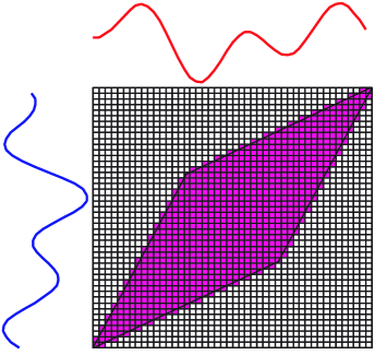
Dynamic Time Warping (DTW) [5] distance is a well-known similarity measure based on shape. It uses a dynamic programming technique to find all possible warping paths, and selects the one with the minimum distance between two time series. To calculate the distance, it first creates a distance matrix, where each element in the matrix is a cumulative distance of the minimum of three surrounding neighbors. Suppose we have two time series, a sequence of length () and a sequence of length (). First, we create an -by- matrix, where every () element of the matrix is the cumulative distance of the distance at () and the minimum of three neighboring elements, where and . We can define the () element, , of the matrix as:
| (1) |
where is the squared distance of and , and is the summation of and the the minimum cumulative distance of three elements surrounding the () element. Then, to find an optimal path, we choose the path that yields a minimum cumulative distance at (), which is defined as:
| (2) |
where is a set of all possible warping paths, is () at element of a warping path, and is the length of the warping path.
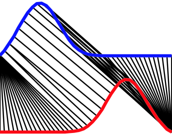
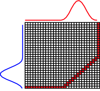
In reality, DTW may not give the best mapping according to our need because it will try its best to find the minimum distance. It may generate the unwanted path. For example, in Figure 1 [5], without global constraint, DTW will find its optimal mapping between the two time series. However, in many cases, this is probably not what we intend, when the two time series are expected to be of different classes. We can resolve this problem by limiting the permissible warping paths using a global constraint. Two well-known global constraints, Sakoe-Chiba band and Itakura Parallelogram [1], and a recent representation, Ratanamahatana-Keogh band (R-K band), have been proposed, Figure 2 [4] shows an example for each type of the constraints.
 |
 |
 |
 |
| (a) | (b) |
 |
|
| (c) | |
2.2 Sakoe-Chiba Band
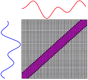
Sakoe-Chiba band (S-C band), shown in Figure 2 (b), is one of the simplest and most popular global constraints, originally introduced to be used for speech community. The width of this global constraint is generally set to be 10% of the time series length. However, recent work [5] has shown that the different sizes of the band can be used towards a more accurate classification. We therefore need to test all possible widths of the global constraint so that the best width could be discovered. An evaluation function is needed to justify the selection. We commonly use accuracy metric (a training accuracy) as a measurement. Table 1 shows an algorithm in finding the best warping window for S-C band by decreasing the band size by 1% in each step. This function receives a set of data as an input, and gives the best warping window (best_band) as an output. Note that if an evaluation value is equal to the best evaluation value, we prefer the smaller warping window size.
| Function [best_band] = BestWarping [] | |
|---|---|
| 1 | best_evaluate = NegativeInfinite; |
| 2 | for ( = 100 to 0) |
| 3 | = S-C band at % width; |
| 4 | = evaluate(); |
| 5 | if ( >= best_evaluate) |
| 6 | best_evaluate = evaluate; |
| 7 | best_band = |
| 8 | endif |
| 9 | endfor |
2.3 Ratanamahatana-Keogh Band
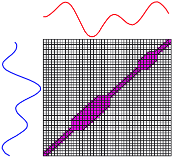
Ratanamahatana-Keogh band (R-K band) [4] is a general model of a global constraint specified by a one-dimensional array , i.e., where is the length of time series, and is the height above the diagonal in direction and the width to the right of the diagonal in direction. Each value is arbitrary, therefore R-K band is also an arbitrary-shape global constraint, as shown in Figure 2 (a). Note that when , where , this R-K band represents the Euclidean distance, and when , where , this R-K band represents the original DTW distance with no global constraint. The R-K band is also able to represent the S-C band by giving all , where is the width of a global constraint. Moreover, the R-K band is a multi band model which can be effectively used to represent one band for each class of data. This flexibility is a great advantage; however, the higher the number of classes, the higher the time complexity, as we have to search through such a large space.
Since determining the optimal R-K band for each training set is highly computationally intensive, a hill climbing and heuristic functions have been introduced to guide which part of space should be evaluated. A space is defined as a segment of a band to be increased or decreased. In the original work, two heuristic functions, accuracy metric and distance metric, are used to evaluate a state. The accuracy metric is evaluated from the training accuracy using leaving-one-out 1-NN, and the distance metric is a ratio of the mean DTW distances of correctly classified and incorrectly classified objects. However, these heuristic functions do not reflect the true quality of a band because empirically, we have found that the resulting bands tend to ‘overfit’ the training data.
Two searching directions are considered, i.e., forward search, and backward search. In forward search, we start from the Euclidean distance (all in equal to 0), and parts of the band are gradually increased in each searching step. In the case where two bands have the same heuristic value, the wider band is selected. On the other hand, in backward search, we start from a very large band (all in equal to , where is the length of time series), and parts of the band are gradually decreased in each searching step. If two bands have the same heuristic value, the tighter band is chosen.
| Function [] = Learning[,] | |
|---|---|
| 1 | = size of ; |
| 2 | = length of data in ; |
| 3 | initialize for = 1 to ; |
| 4 | foreachclass = 1 to |
| 5 | enqueue(1, , ); |
| 6 | endfor |
| 7 | best_evaluate = evaluate(, ); |
| 8 | while !empty() |
| 9 | foreachclass = 1 to |
| 10 | if !empty() |
| 11 | [, ] = dequeue() |
| 12 | ble = adjust(, , ); |
| 13 | if |
| 14 | = evaluate(, ); |
| 15 | if > best_evaluate |
| 16 | best_evaluate = ; |
| 17 | enqueue(, , ); |
| 18 | else |
| 19 | undo_adjustment(, , ); |
| 20 | if ( – ) / 2 |
| 21 | enqueue(, -1, ); |
| 22 | enqueue(, , ); |
| 23 | endif |
| 24 | endif |
| 25 | endif |
| 26 | endif |
| 27 | endfor |
| 28 | endwhile |
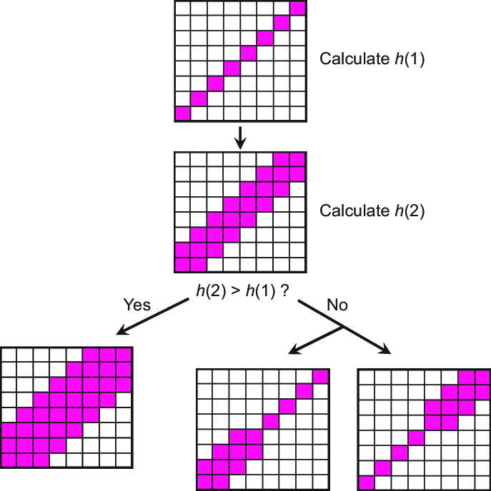
Our learning algorithm starts from first enqueuing the starting- and ending-parts of the R-K Band. In each iteration, these values are dequeued, and used as a boundary for a band increase/decrease. And then the adjusted band is evaluated. If the heuristic value is higher than the current best heuristic value, the same start and end values are enqueued. If not, this part is further divided into two equal subparts before being enqueued, as shown in Figure 3 [4]. The iterations are continued until a termination condition is met. Table 2 shows the pseudo code for this multiple R-K bands learning.
2.4 Silhouette Index
Silhouette index (SI) [7] or Silhouette width is a well-known clustering validity technique, originally used to determine a number of clusters in a dataset. This index measures the ‘quality’ of separation and compactness of a clustered dataset, so the number of cluster is determined by selecting the number that gives maximum index value.
The Silhouette index is based on a compactness-separation measurement which consists of an inter-cluster distance (a distance between two different-cluster data) and an intra-cluster distance (a distance between two same-cluster data). A good clustered dataset means that the dataset has high inter-cluster distance and low intra-cluster distance. In other words, a good clustered dataset is the dataset that different-cluster are well separated, and the same-cluster data are well grouped together. The Silhouette index for each data is defined by the following equation:
| (3) |
| (4) |
| (5) |
where is the Silhouette index of data, is the minimum average distance between the data and each of the different-cluster data, and is the average distance between the data and each of the same-cluster data. In Equations (4) and (5), is a set of all possible clusters, is a set of data in cluster , is the size of , and () is the distance measure function comparing between and data. Note that the ranges between -1 and 1. Having close to 1 means that data is well separated. Global Silhouette index (GS) for a dataset is calculated as follows.
| (6) |
| (7) |
where is the number of clusters, is the Silhouette index for cluster , and is the number of data in cluster . The pseudo code for the Silhouette index function is shown in Table 3.
| Function [] = Silhouette[] | |
|---|---|
| 1 | = size of ; |
| 2 | sum_All = 0; |
| 3 | foreachclass = 1 to |
| 4 | = size of ; |
| 5 | sum_Class = 0; |
| 6 | for = 1 to |
| 7 | = b(); |
| 8 | = a(); |
| 9 | = ( – ) / max(, ); |
| 10 | sum_Class += ; |
| 11 | endfor |
| 12 | sum_All += sum_Class / ; |
| 13 | endfor |
| 14 | = sum_All / ; |
3 Methodology
In this section, we describe our approach, developed from the techniques described in Section 2, i.e., the DTW distance, the best warping window for Sakoe-Chiba band, multiple R-K bands, and the Silhouette index. In brief, our approach consists of 5 major parts: 1) data preprocessing that reduces the length of time series data, 2) our proposed band boundary extraction algorithm, 3) finding the best warping window for Sakoe-Chiba band, 4) our proposed iterative R-K band learning, and 5) prediction for unlabeled data.
Our approach requires three input parameters, i.e., a set of training data , a set of unlabeled data (test data) , the maximum complexity that depends on time and computational resources, and the bound of a warping window size. In data preprocessing step, we could reduce the computational complexity in case of very long time series data using interpolation function, both in training and test data. After that, we try to find the best R-K band by running the band boundary extraction algorithm. The best warping window is calculated and is used as an initial band of our proposed iterative learning. After learning have finished, two R-K bands are compared and the better one is selected. Finally, we calculate a training accuracy and make predictions for the test data using 1-NN with the DTW distance and the best band, enhanced with LB_Keogh lower bound to speed up our classification approach. The prediction result A along with the training accuracy are returned as shown in Table 4.
| Function [, ] = OurApproach[, , , ] | |
|---|---|
| 1 | = length of data in ; |
| 2 | [, , ] = preprocess(, , , ); |
| 3 | [best_band, best_heuristic] = band_extraction(); |
| 4 | = best_warping(, ); |
| 5 | [, ] = iterative_learning(, , , ); |
| 6 | if ( > best_heuristic) |
| 7 | best_heuristic = ; |
| 8 | best_band = ; |
| 9 | endif |
| 10 | = leave_one_out(, best_band); |
| 11 | = predict(, , best_band); |
3.1 Data Preprocessing
Since the classification prediction time may because a major constraint, a data preprocessing step is needed. In this step, we approximate the calculation complexity and try to reduce the complexity exceeding the threshold. Our approximated complexity is mainly based on the number of items in the training data, its length, and the number of heuristic function evaluations. Suppose we have training data with data points in length, we can calculate the complexity by the following equation.
where a logarithm function is added to bring down the value to a more manageable range for users.
To decrease the complexity, we could reduce the length of each individual time series by using typical interpolation function. The new length of time series is set to be the current length divided by two. We keep reducing the time series length until the complexity is smaller than the user’s defined threshold. Table 5 shows the preprocessing steps on a set of training data , a set of unlabeled data , the original length , and the complexity threshold. In this work, we set this threshold value to 9, according to resources and the time constraint for this 24-hour Workshop and Challenge on Time Series Classification.
| Function [, , ] = PreProcess[, , , ] | |
|---|---|
| 1 | = complexity(, ); |
| 2 | set = , = , and = ; |
| 3 | while ( > ) |
| 4 | = / 2; |
| 5 | = interpolate(, ); |
| 6 | = interpolate(, ); |
| 7 | = complexity(, ); |
| 8 | endwhile |
| Function [best_band, best_heuristic] = BandExtraction[] | |
|---|---|
| 1 | = size of ; |
| 2 | = length of data in ; |
| 3 | initialize path_matrix = new array [][]; |
| 4 | initialize for , , and |
| 5 | foreachclass ( = 1 to ) |
| 6 | = size of ; |
| 7 | for ( = 1 to ) |
| 8 | for ( = 1 to ) |
| 9 | if ( != ) |
| 10 | = dtw_path(, ); |
| 11 | for (all point in ) |
| 12 | path_matrix[][]++; |
| 13 | endfor |
| 14 | endif |
| 15 | endfor |
| 16 | endfor |
| 17 | for (i = 0 to ) |
| 18 | [] = maximum warping path at |
| 19 | [] = mean warping path at |
| 20 | [] = mode warping path at |
| 21 | endfor |
| 22 | end |
| 23 | [best_band, best_heuristic] = bestband(, , ); |
 |
 |
 |
| (a) | ||
 |
 |
|
| (b) | (c) |
3.2 Boundary Band Extraction
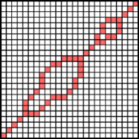
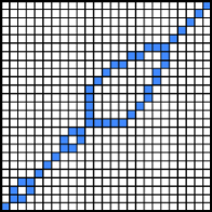
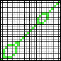
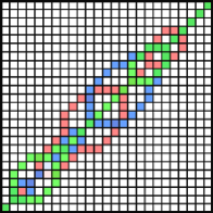
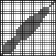
Since the multi R-K band model allows a learning algorithm to create a different band for each different class. This boundary band extraction algorithm is derived from a simple intuition for each of the same-class data, we first calculate all their DTW distances, save all the warping paths, and plot those paths on a matrix (called a path matrix). After that, we will determine an appropriate R-K band. For each of this R-K band, the value is set to be the maximum between height above the diagonal in direction and width to the right of the diagonal in direction in the path matrix. We repeat these steps to every possible class in the dataset; we call this R-K band a . Similarly, the band extraction is performed using mean average and mode instead of the maximum, resulting in a and a , respectively. Figure 4 illustrates the steps in creating a . From these calculations, three multiple R-K bands are generated. The evaluation function is used to select the best band to be returned as an output of this algorithm. Table 6 shows the band boundary extraction algorithm on a set of training data and return the best R-K band and the best heuristic value.
| Function [] = BestWarping[,] | |
|---|---|
| 1 | = size of ; |
| 2 | best_heuristic = NegativeInfinite; |
| 3 | for ( = to 0) |
| 4 | = S-C Band at % width; |
| 5 | = evaluate(); |
| 6 | if ( > best_heuristic) |
| 7 | best_heuristic = ; |
| 8 | = ; |
| 9 | endif |
| 10 | endfor |
3.3 Finding the Best Warping Window
In this step, we try to achieve the best warping window of Sakoe-Chiba band to be an input of our proposed iterative R-K band learning. This function is slightly different from the original one in that we bound the maximum width of the warping window and we use our evaluation function (heuristic function) instead of the typical training accuracy. A simple pseudo code is described in Table 7 below. A set of training data and a maximum warping window size are required in discovering the best warping window .
| Function [] = IterativeLearning[, , , ] | |
|---|---|
| 1 | initialize best_bandi for i = 0 to equals to R% of L |
| 2 | threshold = L / 2; |
| 3 | best_heuristic = evaluate(T, band); |
| 4 | while (threshold) < 1 |
| 5 | fw_band = forward_learning(T, , , ); |
| 6 | bw_band = backward_learning(, , , ); |
| 7 | fw_heuristic = evaluate(, fw_band); |
| 8 | bw_heuristic = evaluate(, bw_band); |
| 9 | = maximum heuristic value band; |
| 10 | = maximum heuristic value; |
| 11 | if = best_heuristic |
| 12 | = / 2; |
| 13 | endif |
| 14 | endwhile |
3.4 Iterative Band Learning
The iterative R-K band learning is extended from the original learning that it will repeat the learning again and again until a heuristic value no longer increases. In the first step, we initialize all the multi R-K bands with % Sakoe-Chiba band, where is the output from the best finding warping window algorithm. We also set a learning threshold to be half of the time series length, and the initial bands are evaluated
In each iteration, our proposed algorithm learns a new R-K band starting with the previous R-K band learning result both in forward and backward direction. We also run both forward and backward learning and select the best band which gives a higher heuristic value. If the heuristic value is the same as the best heuristic value, the threshold is divided by two; otherwise we update the best heuristic value. We repeat these steps until the threshold falls below 1. Table 8 shows our proposed algorithm, iterative R-K band learning, which requires a set of training data , a best warping window , the length of time series , and the bound of warping window.
| Function [] = ProposedLearning[, , , ] | |
|---|---|
| 1 | = length of data in T; |
| 2 | foreachclass i = 1 to c |
| 3 | enqueue(1, L, i, Queue); |
| 4 | endfor |
| 5 | best_heuristic = evaluate(T, band); |
| 6 | while !empty(Queue) |
| 7 | [start, end, label] = randomly_dequeue(Queue) |
| 8 | adjustable = adjust(bandlabel, start, end, bound); |
| 9 | if adjustable |
| 10 | heuristic = evaluate(T, band); |
| 11 | if heuristic > best_heuristic |
| 12 | best_heuristic = heuristic; |
| 13 | enqueue(start, end, label, Queue); |
| 14 | else |
| 15 | undo_adjustment(bandlabel, start, end); |
| 16 | if (start – end) / 2 threshold |
| 17 | enqueue(start, mid-1, label, Queue); |
| 18 | enqueue(mid, end, label, Queue); |
| 19 | endif |
| 20 | endif |
| 21 | endif |
| 22 | endwhile |
We have modified the original multi R-K bands learning by changing its data structure. We replace multi queues, which are originally assigned for each class by only one single queue with an addition parameter label to each start-end object. This new queue will draw an object randomly instead of last-in-first-out (LIFO) manner. In addition, we also change an adjustment function by adding a new parameter bound to limit forward learning not to increase the band’s size exceeding limited bound. Table 9 shows the proposed R-K band learning on a set of training data , a learning threshold, an initial band, and the bound of warping window.
3.5 Evaluation Function
From Section 2.4, we have briefly described the utility and the algorithm of the Silhouette index. This index is commonly used to measure the quality of a clustered dataset; however, we can utilize this Silhouette index as a heuristic function to measure the quality of a distance measure as well. The DTW distance with multi R-K bands is a distance measure that requires one additional parameter, , specifying the R-K band to be used (since the multi R-K bands contain one band for each class). Table 10 shows the evaluation function derived from the original Silhouette index.
| (8) |
| (9) |
| (10) |
| Function [] = Evaluate[,] | |
|---|---|
| 1 | = size of ; |
| 2 | sum_All = 0; |
| 3 | foreachclass ( = 1 to ) |
| 4 | = size of ; |
| 5 | sum_Class = 0; |
| 6 | for ( = 1 to ) |
| 7 | = b(, ); |
| 8 | = a(, ); |
| 9 | = ( – ) / max(, ); |
| 10 | sum_Class += ; |
| 11 | endfor |
| 12 | sum_All += sum_Class / ; |
| 13 | endfor |
| 14 | = sum_All / ; |
3.6 Data Prediction
After the best multi R-K bands are discovered, we use 1-Nearest Neighbor as a classifier and the Dynamic Time Warping distance measure with these best R-K bands for prediction in the test data to predict a set of unlabeled data. The LB_Keogh lower bound is also used to speed up the DTW computation.
4 Experimental Evaluation
To evaluate the performance, we use our approach, described in Section 3, to classify all 20 contest datasets, and then send our predicted results and the expected accuracies to the contest organizer. The results are calculated by the contest organizer and subsequently sent back to us.
4.1 Datasets
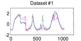
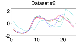
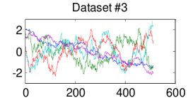
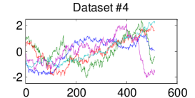
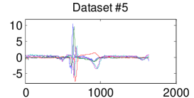
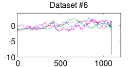
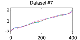
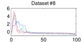
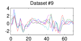
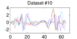
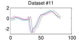
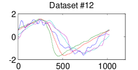
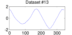
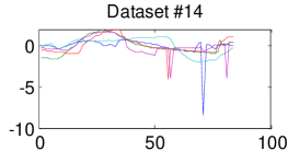
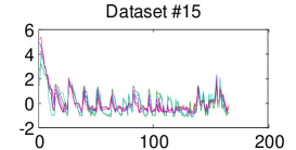
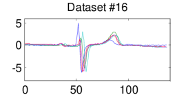
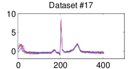
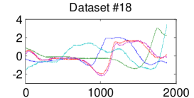
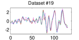
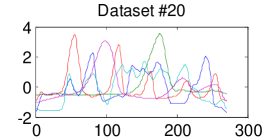
We use the datasets from the Workshop and Challenge on Time Series Classification, held in conjunction with the thirteenth SIGKDD 2007 conference. The datasets are from very diverse domains (e.g., stock data, medical data, etc.); some are from real-world problems, and some are synthetically generated. The amount of training data and its length in each dataset also vary from the size of 20 to 1000 training instances and the length of 30 to 2000 data points. In addition, all data are individually normalized using Z-normalization. Examples of each dataset are shown in Figure 5, and the datasets’ properties are shown in Table 11.
 |
 |
 |
 |
 |
 |
 |
 |
 |
 |
 |
 |
 |
 |
 |
 |
 |
 |
 |
 |
| Dataset | #Classes | Training | Test | Length of each |
|---|---|---|---|---|
| data size | data size | time series | ||
| 1 | 8 | 55 | 2345 | 1024 |
| 2 | 2 | 67 | 1029 | 24 |
| 3 | 2 | 367 | 1620 | 512 |
| 4 | 2 | 178 | 1085 | 512 |
| 5 | 4 | 40 | 1380 | 1639 |
| 6 | 5 | 155 | 308 | 1092 |
| 7 | 6 | 25 | 995 | 398 |
| 8 | 10 | 381 | 760 | 99 |
| 9 | 2 | 20 | 601 | 70 |
| 10 | 2 | 27 | 953 | 65 |
| 11 | 2 | 23 | 1139 | 82 |
| 12 | 3 | 1000 | 8236 | 1024 |
| 13 | 4 | 16 | 306 | 345 |
| 14 | 2 | 20 | 1252 | 84 |
| 15 | 3 | 467 | 3840 | 166 |
| 16 | 2 | 23 | 861 | 136 |
| 17 | 2 | 73 | 936 | 405 |
| 18 | 7 | 100 | 550 | 1882 |
| 19 | 12 | 200 | 2050 | 131 |
| 20 | 15 | 267 | 638 | 270 |
4.2 Results
The predicted result is generated after running our algorithm to find the best R-K band within the competition’s 24-hour time constraint. More specifically, the predicted accuracy is calculated by computing leaving-one-out cross validation on the training dataset. Table 12 shows our predicted accuracies and testing accuracies for all 20 datasets which are calculated and are returned to the contest organizer. Because of the small number of training data, the predicted accuracy and the test accuracy are different in some cases.
| Dataset | Predicted accuracy | Test accuracy |
|---|---|---|
| 1 | 0.9636 | 0.6505 |
| 2 | 0.9403 | 0.9161 |
| 3 | 0.4714 | 0.3491 |
| 4 | 0.9494 | 0.9231 |
| 5 | 0.9500 | 0.8537 |
| 6 | 0.1871 | 0.6099 |
| 7 | 1.0000 | 0.8714 |
| 8 | 0.7428 | 0.9346 |
| 9 | 0.9500 | 0.8488 |
| 10 | 0.8519 | 0.8507 |
| 11 | 0.9565 | 0.8489 |
| 12 | 0.8570 | 0.8353 |
| 13 | 0.9375 | 0.7250 |
| 14 | 0.9000 | 0.9276 |
| 15 | 0.6017 | 0.4435 |
| 16 | 0.7391 | 0.8645 |
| 17 | 0.8904 | 0.9346 |
| 18 | 0.2900 | 0.5049 |
| 19 | 0.9500 | 0.9660 |
| 20 | 0.6966 | 0.9275 |
5 Conclusion
In this work, we propose a new efficient time series classification algorithm based on 1-Nearest Neighbor classification using the Dynamic Time Warping distance with multi R-K bands as a global constraint. To select the best R-K band, we use our two proposed learning algorithms, i.e., band boundary extraction algorithm and iterative learning. Silhouette index is used as a heuristic function for selecting the band that yields the best prediction accuracy. The LB_Keogh lower bound is also used in data prediction step to speed up the computation.
6 Acknowledgments
We would like to thank the Scientific PArallel Computer Engineering (SPACE) Laboratory, Chulalongkorn University for providing a cluster we have used in this contest.
References
- [1] Fumitada Itakura. Minimum prediction residual principle applied to speech recognition. IEEE Transactions on Acoustics, Speech, and Signal Processing, 23(1):67–72, 1975.
- [2] Eamonn J. Keogh and Chotirat Ann Ratanamahatana. Exact indexing of dynamic time warping. Knowledge and Information Systems, 7(3):358–386, 2005.
- [3] Alex Nanopoulos, Rob Alcock, and Yannis Manolopoulos. Feature-based classification of time-series data. Information Processing and Technology, pages 49–61, 2001.
- [4] Chotirat Ann Ratanamahatana and Eamonn J. Keogh. Making time-series classification more accurate using learned constraints. In Proceedings of the Fourth SIAM International Conference on Data Mining (SDM 2004), pages 11–22, Lake Buena Vista, FL, USA, April 22-24 2004.
- [5] Chotirat Ann Ratanamahatana and Eamonn J. Keogh. Three myths about dynamic time warping data mining. In Proceedings of 2005 SIAM International Data Mining Conference (SDM 2005), pages 506–510, Newport Beach, CL, USA, April 21-23 2005.
- [6] Juan José Rodríguez and Carlos J. Alonso. Interval and dynamic time warping-based decision trees. In Proceedings of the 2004 ACM Symposium on Applied Computing (SAC 2004), pages 548–552, Nicosia, Cyprus, March 14-17 2004.
- [7] Peter Rousseeuw. Silhouettes: a graphical aid to the interpretation and validation of cluster analysis. Journal of Computational and Applied Mathematics, 20(1):53–65, 1987.
- [8] Hiroaki Sakoe and Seibi Chiba. Dynamic programming algorithm optimization for spoken word recognition. IEEE Transactions on Acoustics, Speech, and Signal Processing, 26(1):43–49, 1978.
- [9] Yi Wu and Edward Y. Chang. Distance-function design and fusion for sequence data. In Proceedings of the 2004 ACM CIKM International Conference on Information and Knowledge Management (CIKM 2004), pages 324–333, Washington, DC, USA, November 8-13 2004.