Learning Efficient Multi-Agent Cooperative Visual Exploration
Abstract
We tackle the problem of cooperative visual exploration where multiple agents need to jointly explore unseen regions as fast as possible based on visual signals. Classical planning-based methods often suffer from expensive computation overhead at each step and a limited expressiveness of complex cooperation strategy. By contrast, reinforcement learning (RL) has recently become a popular paradigm for tackling this challenge due to its modeling capability of arbitrarily complex strategies and minimal inference overhead. In this paper, we extend the state-of-the-art single-agent visual navigation method, Active Neural SLAM (ANS), to the multi-agent setting by introducing a novel RL-based planning module, Multi-agent Spatial Planner (MSP). MSP leverages a transformer-based architecture, Spatial-TeamFormer, which effectively captures spatial relations and intra-agent interactions via hierarchical spatial self-attentions. In addition, we also implement a few multi-agent enhancements to process local information from each agent for an aligned spatial representation and more precise planning. Finally, we perform policy distillation to extract a meta policy to significantly improve the generalization capability of final policy. We call this overall solution, Multi-Agent Active Neural SLAM (MAANS). MAANS substantially outperforms classical planning-based baselines for the first time in a photo-realistic 3D simulator, Habitat. Code and videos can be found at https://sites.google.com/view/maans.
1 Introduction
Visual exploration (Ramakrishnan et al., 2021) is an important task for building intelligent embodied agents and has been served as a fundamental building block for a wide range of applications, such as scene reconstruction (Anguelov et al., 2010; Isler et al., 2016), autonomous driving (Bresson et al., 2017), disaster rescue (Kleiner et al., 2006) and planetary exploration (Tagliabue et al., 2020). In this paper, we consider a multi-agent exploration problem, where multiple homogeneous robots simultaneously explore an unknown spatial region via visual and sensory signals in a cooperative fashion. The existence of multiple agents enables complex cooperation strategies to effectively distribute the workload among different agents, which could lead to remarkably higher exploration efficiency than the single-agent counterpart.
Planning-based solutions have been widely adopted for robotic navigation problems for both single-agent and multi-agent scenarios (Burgard et al., 2005; Savinov et al., 2019; Umari & Mukhopadhyay, 2017). Planning-based methods require little training and can be directly applied to different scenarios. However, these methods often suffer from limited expressiveness capability on coordination strategies, require non-trivial hyper-parameter tuning for each test scenario, and are particularly time-consuming due to repeated re-planning at each decision step. By contrast, reinforcement learning (RL) has been promising solution for a wide range of decision-making problems (Lillicrap et al., 2015; Mnih et al., 2013), including various visual navigation tasks (Chaplot et al., 2020a; Chen et al., 2019; Savinov et al., 2019). An RL-based agent is often parameterized as a deep neural network and directly produces actions based on raw sensory signals. Once a policy is well trained by an RL algorithm, the robot can capture arbitrarily complex strategies and produce real-time decisions with efficient inference computation (i.e., a single forward-pass of neural network).
However, training effective RL policies can be particularly challenging. This includes two folds: (1) learning a cooperative strategy over multiple agents in an end-to-end manner becomes substantially harder thanks to an exponentially large action space and observation space when tackling the exploration task based on visual signals; (2) RL policies often suffer from poor generalization ability to different scenarios or team sizes compared with classical planning-based approaches. Hence, most RL-based visual exploration methods focus on the single-agent case (Chaplot et al., 2020a; Chen et al., 2019; Savinov et al., 2019) or only consider a relatively simplified multi-agent setting (like maze or grid world (Wakilpoor et al., 2020)) of a fixed number of agents (Liu et al., 2021b).
In this work, we develop Multi-Agent Active Neural SLAM (MAANS), the first RL-based solution for cooperative multi-agent exploration that substantially outperforms classical planning-based methods in a photo-realistic physical simulator, Habitat (Savva et al., 2019). MAANS extends the single-agent Active Neural SLAM method (Savinov et al., 2019) to the multi-agent setting. In MAANS, an agent consists of 4 components, a neural SLAM module, a planning-based local planner, a local policy for control, and the most critical one, a novel Multi-agent Spatial Planner (MSP). which is an RL-trained planning module that can capture complex intra-agent interactions via a self-attention-based architecture, Spatial-TeamFormer, and produce effective navigation targets for a varying number of agents. We also implement a map refiner to align the spatial representation of each agent’s local map, and a map merger, which enables the local planner to perform more precise sub-goal generation over a manually combined approximate 2D map. Finally, instead of directly running multi-task RL over all the training scenes, we first train a single policy on each individual scene and then use policy distillation to extract a meta policy, leading to a much improved generalization capability,
We conduct thorough experiments in a photo-realistic physical simulator, Habitat, and compare MAANS with a collection of classical planning-based methods and RL-based variants. Empirical results show that MAANS has a 20.56% and 7.99% higher exploration efficiency on training and testing scenes than the best planning-based competitor. The learned policy can further generalize to novel team sizes in a zero-shot manner as well.
2 Related Work
2.1 Visual Exploration
In classical visual exploration solutions, an agent first locates its position and re-constructs the 2D map based on its sensory signals, which is formulated as Simultaneous Localization and Mapping (SLAM) (Fuentes-Pacheco et al., 2015). Then a search-based planning algorithm will be adopted to generate valid exploration trajectories. Representative variants include frontier-based methods (Umari & Mukhopadhyay, 2017; Yamauchi, 1997a; Yu et al., 2021b), which always choose navigation targets from the explored region, and sampling-based methods (Li, 2020), which generate goals via a stochastic process. In addition to the expensive search computation for planning, these methods do not involve learning and thus have limited representation capabilities for particularly challenging scenarios. Hence, RL-based methods have been increasingly popular for their training flexibility and strong expressiveness power. Early methods simply train navigation policies in a purely end-to-end fashion (Chen et al., 2019; Jain et al., 2019) while recent works start to incorporate the inductive bias of a spatial map structure into policy representation by introducing a differentiable spatial memory (Henriques & Vedaldi, 2018; Mousavian et al., 2019; Parisotto & Salakhutdinov, 2018), semantic prior knowledge (Liu et al., 2021b) or learning a topological scene graph (Bhatti et al., 2016; Chaplot et al., 2020c; Yang et al., 2018).
The Active Neural SLAM (ANS) method (Chaplot et al., 2020a) is the state-of-the-art framework for single-agent visual exploration, which takes advantage of both planning-based and RL-based techniques via a modular design (details in Sec. 3.2). There are also follow-up enhancements based on the ANS framework, such as improving map reconstruction with occupancy anticipation (Ramakrishnan et al., 2020) and incorporating semantic signals into the reconstructed map for semantic exploration (Chaplot et al., 2020b). Our MAANS can be viewed as a multi-agent extension of ANS with a few multi-agent-specific components.
2.2 Multi-agent Cooperative Exploration
There have been works extending planning-based visual exploration solutions to the multi-agent setting by introducing handcraft planning heuristics over a shared reconstructed 2D map (Čáp et al., 2013; Cohen, 1996; Desaraju & How, 2011; Hu et al., 2020; Nazif et al., 2010; Patel et al., ; Wurm et al., 2008). However, due to the lack of learning, these methods may have the limited potential of capturing non-trivial multi-agent interactions in challenging domains. By contrast, multi-agent reinforcement learning (MARL) has shown its strong performances in a wide range of domains (Nguyen et al., 2020), so many works have been adopting MARL to solve challenging cooperative problems. Representative works include value decomposition for approximating credit assignment (Rashid et al., 2018; Sunehag et al., 2018), learning intrinsic rewards to tackle sparse rewards (Iqbal & Sha, 2019b; Liu et al., 2021a; Wang* et al., 2020) and curriculum learning (Long et al., 2020; Wang et al., 2020).
However, jointly optimizing multiple policies makes multi-agent RL training remarkably more challenging than its single-agent counterpart. Hence, these end-to-end RL methods either focus on much simplified domains, like grid world or particle world (Wakilpoor et al., 2020), or still produce poor exploration efficiency compared with classical planning-based solutions. Our MAANS framework adopts a modular design and is the first RL-based solution that significantly outperforms classical planning-based baselines in a photo-realistic physical environment.
Finally, we remark that MAANS utilizes a centralized global planner MSP, which assumes perfect communication between agents. There are also works on multi-agent cooperation with limited or constrained communication (Jiang & Lu, 2018; Peng et al., 2017; Sukhbaatar et al., 2016; Foerster et al., 2016; Jain et al., 2019; Wang et al., 2021; Zhu et al., 2021), which are parallel to our focus.
2.3 Size-Invariant Representation Learning
There has been rich literature in deep learning studying representation learning over an arbitrary number of input entities in deep learning (Zhang et al., 2019a; b). In MARL, the self-attention mechanism (Vaswani et al., 2017) has been the most popular policy architecture to tackle varying input sizes (Duan et al., 2017; Jiang et al., 2018; Ryu et al., 2020; Wang et al., 2018) or capture high-order relations (Iqbal & Sha, 2019a; Malysheva et al., 2018; Yang et al., 2018; Zambaldi et al., 2018). A concurrent work (Wang et al., 2021) also considers the zero-shot team-size adaptation in the photo-realistic environment by learning a simple attention-based communication channel between agents. By contrast, our works develop a much expressive network architecture, Spatial-TeamFormer, which adopts a hierarchical self-attention-based architecture to capture both intra-agent and spatial relationships and results in substantially better empirical performance (see Section 5.4.2). Besides, parameter sharing is another commonly used technique in MARL for team-size generalization, which has been also shown to help reduce nonstationarity and accelerate training (Chu & Ye, 2017; Terry et al., 2020). Our work follows this paradigm as well.
3 Preliminary
3.1 Task Setup
We consider a multi-agent coordination indoor active SLAM problem, in which a team of agents needs to cooperatively explore an unknown indoor scene as fast as possible. At each timestep, each agent performs an action among Turn Left, Turn Right and Forward, and then receives an RGB image through a camera and noised pose change through a sensor, which is provided from the Habitat environment. We consider a decision-making setting by assuming perfect communication between agents. The objective of the task is to maximize the accumulative explored area within a limited time horizon.
3.2 Active Neural SLAM
The ANS framework (Chaplot et al., 2020a) consists of 4 parts: a neural SLAM module, a RL-based global planner, a planning-based local planner and a local policy. The neural SLAM module, which is trained by supervised learning, takes an RGB image, the pose sensory signals, and its past outputs as inputs, and outputs an updated 2D reconstructed map and a current pose estimation. Note that in ANS, the output 2D map only covers a neighboring region of the agent location and always keeps the agent at the egocentric position. For clarification, we call this raw output map from the SLAM module a agent-centric local map.
The global planner in ANS takes in an augmented agent-centric local map, which includes channels indicating explored regions, unexplored regions and obstacles and the history trajectory, as its input, and outputs two real numbers from two Gaussian distributions denoting the coordinate of the long-term goal. This global planner is parameterized as a CNN policy and trained by the PPO algorithm (Schulman et al., 2017). The local planner performs classical planning, i.e., Fast Marching Method (FMM) (Sethian, 1996), over the agent-centric local map towards a given long-term goal, and outputs a trajectory of short-term sub-goals. Finally, the local policy produces actions given an RGB image and a sub-goal and is trained by imitation learning.
With the advantage of the modeling capability of arbitrarily complex strategy in RL, an RL-based global planner which determines the global goals encourages exploration faster. To apply RL training, we model the problem as a decentralized partially observable Markov decision process (Dec-POMDP). Dec-POMDP is parameterized by . is the number of agents. is the state space, is the joint action space. is agent ’s observations at state . defines the transition probability from state to state via joint action . is the shared reward function. is the discount factor. The objective function is . In this task, the policy generates a global goal for each agent every decision-making step. The shared reward function is defined as the accumulative environment reward every global goal planning step.
4 Methodology
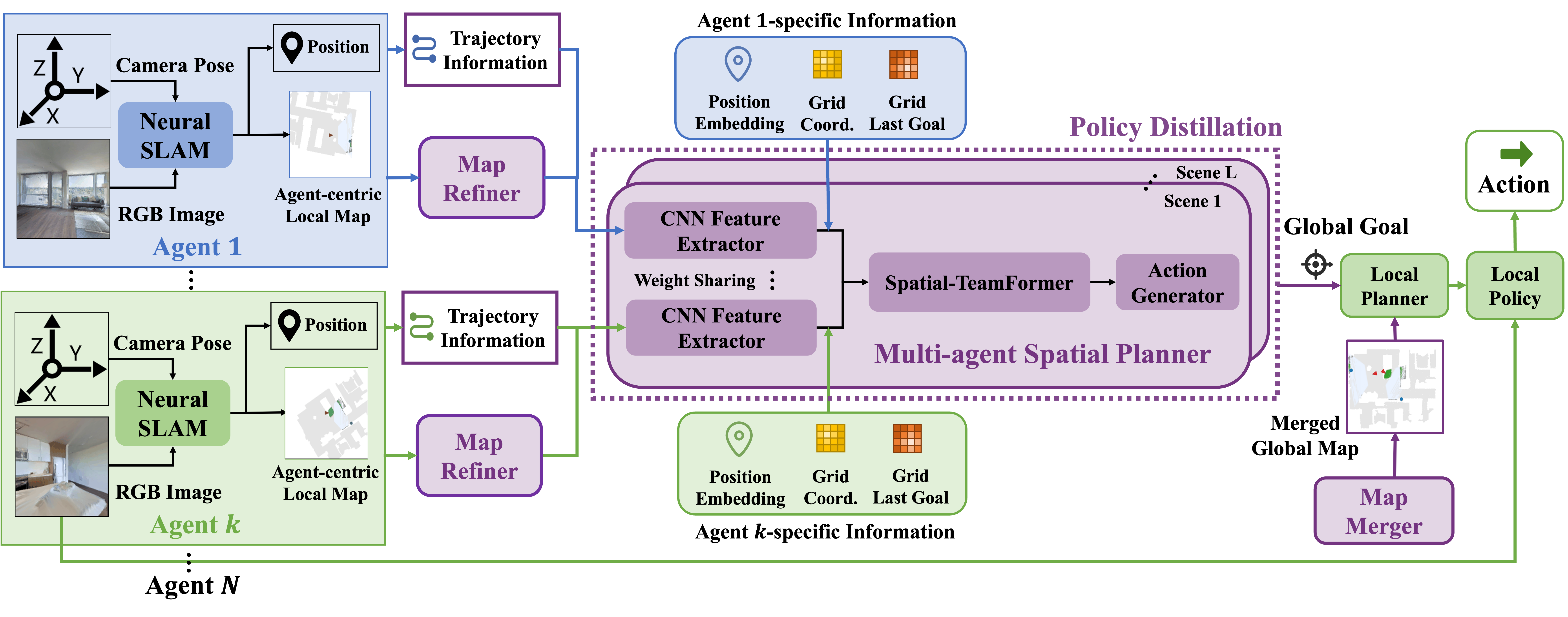
The overview of MAANS is demonstrated in Fig. 1, where each agent is presented in a modular structure. When each agent receives the visual and pose sensory signals from the environment, the Neural SLAM module corrects the sensor error and performs SLAM in order to build a top-down 2D occupancy map that includes explored area and discovered obstacles. Then we use a Map Refiner to rotate each agent’s egocentric local map to a global coordinate system. We augment these refined maps with each agent’s trajectory information and feed these spatial inputs along with other agent-specific information to our core planning module, Multi-agent Spatial Planner (MSP) to generate a global goal as the long-term navigation target for each individual agent. We remark that only estimated geometric information is utilized in this map fusion process. To effectively reach a global goal, the agent first plans a path to this long-term goal in a manually merged global map using FMM and generates a sequence of short-term sub-goals. Finally, given a short-term sub-goal, a Local Policy outputs the final navigation action based on the visual input and the relative spatial distance as well as the relative angle to the sub-goal.
Note that the Neural SLAM module and the Local Policy do not involve multi-agent interactions, so we directly reuse these two modules from ANS (Savinov et al., 2019). We fix these modules throughout training and only train the planning module MSP using the MAPPO algorithm (Yu et al., 2021a), a multi-agent variant of PPO (Schulman et al., 2017). Hence, the actual action space for training MSP is the spatial location of the global goal.
4.1 Multi-agent Spatial Planner
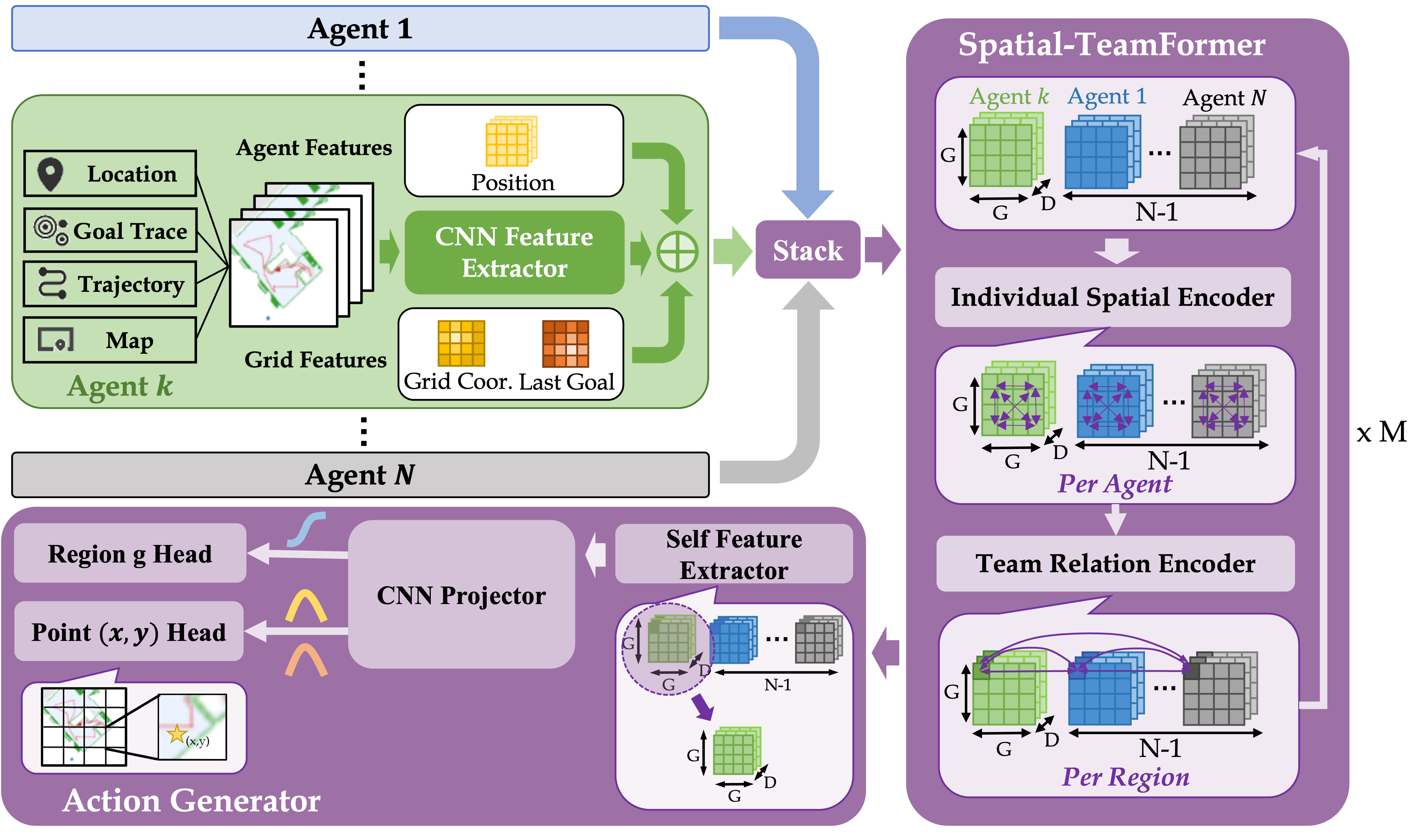
Multi-agent Spatial Planner (MSP) is the core component in MAANS, which could perform planning for an arbitrary number of agents. The full workflow of MSP is shown in Fig. 2. MSP first applies a weight-shared CNN feature extractor to extract spatial feature maps from each agent’s local navigation trajectory and then fuses team-wise information with hierarchical transformer-based network architecture, Spatial-TeamFormer. Finally, an action generator will generate a spatial global goal based on the features from Spatial-TeamFormer. Suppose there are a total of agents and the current decision-making agent has ID . We will describe how agent generates its long-term goal via the 3 parts in MSP in the following content. Note that due to space constraints, we only present the main ideas while more computation details can be found in Appendix A.4.
4.1.1 CNN Feature Extractor
For every single agent, we use its current location, movement trajectory, previous goal, goal history, self-occupancy map and obstacle map as inputs and convert them to a 2D map with 6 channels over a global coordinate system. We adopt a weight-shared CNN network with 5 layers to process each agent’s input map, which produces a feature map with channels. corresponds to the discretization level of the scene. We choose in our work, leading to grids corresponding to different spatial regions in the underlying indoor scene.
Besides CNN spatial maps, we also introduce additional features, including agent-specific embeddings of its current position and grid features, i.e., the embeddings of the relative coordinate of each grid to the agent position as well as the embedding of the previous global goal.
4.1.2 Spatial-TeamFormer
With a total of extracted feature maps, we aim to learn a team-size-invariant spatial representation over all the agents. Transformer has been a particularly popular candidate for learning invariant representations, but it may not be trivially applied in this case. Standard Transformer model in NLP (Vaswani et al., 2017) tackles 1-dimensional text inputs, which ignores the spatial structure of input features. Visual transformers (Dosovitskiy et al., 2020) capture spatial relations well by performing spatial self-attention. However, we have a total of spatial inputs from the entire team.
Hence, we present a specialized architecture to jointly leverage intra-agent and spatial relationships in a hierarchical manner, which we call Spatial-TeamFormer. A Spatial-Teamformer block consists of two layers, i.e., an Individual Spatial Encoder for capturing spatial features for each agent, and a Team Relation Encoder for reasoning cross agents. Similar to visual transformer (Dosovitskiy et al., 2020), Individual Spatial Encoder focuses only on spatial information by performing a spatial self-attention over each agent’s own spatial map without any cross-agent computation. By contrast, Team Relation Encoder completely focuses on capturing team-wise interactions without leveraging any spatial information. In particular, for each of the grid, Team Relation Encoder extracts the features w.r.t. that grid from the agents and performs a standard transformer over these features. We can further stack multiple Spatial-TeamFormer blocks for even richer interaction representations.
We remark that another possible alternative to Spatial-TeamFormer is to simply use a big transformer over the aggregated features. Such a naive solution is substantially more expensive to compute ( time complexity) than Spatial-TeamFormer ( time complexity), which may also incur significant learning difficulty in practice (see Section 5.4.3).
4.1.3 Action Generator
The Action Generator is the final part of MSP, which outputs a long-term global goal over the reconstructed map. Since spatial-TeamFormer produces a total of rich spatial representation, which can be denoted as , we take the first grid, which is the feature map of the current agent, to derive a single team-size-invariant representation.
In order to produce accurate global goals, we adopt a spatial action space with two separate action heads, i.e., a discrete region head for choosing a region from the discretized grids, and a continuous point head for outputing a coordinate , indicating the relative position of the global goal within the selected region . To compute the action probability for , we compute a spatial softmax operator over all the grids while to ensure the scale of is bounded between 0 and 1, we apply a sigmoid function before outputting the value of . We remark that such a spatial design of action space is beneficial since it alleviates the problem of multi-modal issue of modeling potential "good" goals, which could not be simply represented by a simple normal distribution as used in (Chen et al., 2019) (see Section 5.4.2).
4.2 Map Refiner for Aligned 2D Maps
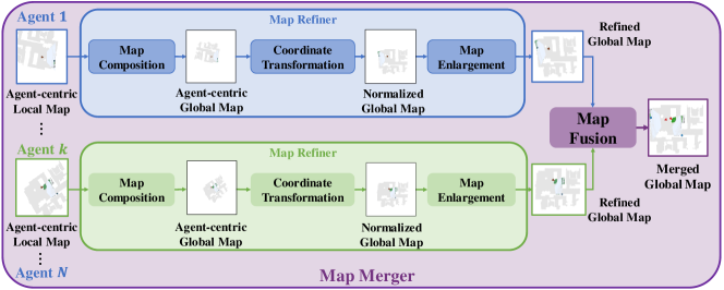
We develop a map refiner to ensure all the maps from the neural SLAM module are within the same coordinate system. The workflow is shown as the blue and green part in Fig. 3. The map refiner first composes all the past agent-centric local maps to recover the agent-centric global map. Then, we transform the coordinate system based on the pose estimates to normalize the global maps from all the agents w.r.t. the same coordinate system. Note that when an agent explores the border of the house, the agent-centric local map often covers a large portion of invisible region. As a result, the normalized global map will accordingly contain a large unexplorable boundary surrounding the actual explorable house region. To ensure the feature extractor in MSP concentrates only on the viable part and also induce a more focused spatial action space, we crop the unexplorable boundary of the normalized map and enlarge the house region as our final refined map.
4.3 Map Merger for Improved Local Planning
The local planner from ANS plans sub-goals on the agent-centric local map, while in our setting, we can also leverage the information from other agents to plan over a more accurate map. The diagram of map merger is shown in Fig. 3. After obtaining enlarged global maps via the map refiner, the map merger simply integrates all these maps by applying a max-pooling operator for each pixel location. That is, for each pixel in the merged global map, the probability of it being an obstacle is the maximum value at that pixel over all individual enlarged global maps. We remark that the artificial merged global map is only utilized in the local planner, but not in the global planner MSP. We empirically observe that having a coarse merged map produces better short-term local goal while such an artificial map is not sufficient for accurate global planning. (see Section 5.4.2)
4.4 Policy Distillation for Improved Generalization
The common training paradigm for visual exploration is multi-task learning, i.e., at each training episode, a random training scene or team size is sampled and all collected samples are aggregated for policy optimization (Chaplot et al., 2020a; Chen et al., 2019). However, we empirically observe that different Habitat scenes and team sizes may lead to drastically different exploration difficulties. During training, gradients from different configurations may negatively impact each other. Similar observations have been also reported in the existing literature (Hessel et al., 2019; Teh et al., 2017). We use policy distillation to tackle this problem. Therefore, we adopt a two-phase distillation-based solution: in the first phase, we train separate policies for representative training scenes with a fixed team size, i.e., we choose in our experiments in the second phase, we learn another policy with agents to distill the collection of pretrained policies over different training scenes and directly measure the generalization ability of this distillation policy to novel scenes and different team sizes. More specifically, for the -th training scene, we first learn a specialized teacher policy given state with parameter , where denotes the region output and is the point head output. Then we train another distillation policy by simply running a dagger-style imitation learning, i.e., randomly rollout trajectories w.r.t. the distillation policy and imitate the output from the specific teacher policy. Since the region action is discrete, we adopt a KL-divergence-based loss function while for the continuous point action , a squared difference loss between the teacher policy and distillation policy is optimized.
5 Experiment Results
5.1 Experiment Setting
We adopt scene data from the Gibson Challenge dataset (Xia et al., 2018b) while the visual signals and dynamics are simulated by the Habitat simulator (Savva et al., 2019). Although Gibson Challenge dataset provides training and validation scenes, we discard scenes that are not appropriate for our task, such as scenes that have large disconnected regions or multiple floors so that the agents are not possible to achieve 90% coverage of the entire house. Then we categorize the remaining scenes into training scenes and testing scenes. We consider agents in our experiments. Every RL training is performed with training episodes over 3 random seeds. Each evaluation score is expressed in the format of “mean (standard deviation)”, which is averaged over a total of 300 testing episodes, i.e., 100 episodes per random seed. More details are deferred to Appendix E.
5.2 Evaluation Metrics
We take 3 metrics to examine the exploration efficiency:
-
1.
Coverage: Coverage represents the ratio of areas explored by the agents to the entire explorable space in the indoor scene at the end of the episode. Higher Coverage implies more effective exploration.
-
2.
Steps: Steps is the number of timesteps used by agents to achieve a coverage ratio of within an episode. Fewer Steps implies faster exploration.
-
3.
Mutual Overlap: For effective collaboration, each agent should visit regions different from those explored by its teammates. We report the average overlapping explored area over each pair of agents when the coverage ratio reaches 90%. Mutual Overlap denotes the normalized value of this metric. Lower Mutual Overlap suggests better multi-agent coordination.
5.3 Baselines
We first adapt single-agent planning-based methods, namely Nearest (Yamauchi, 1997a), Utility (Juliá et al., 2012), and RRT (Umari & Mukhopadhyay, 2017), to our problems by planning on the merged global map. The 3 planning-based baselines are frontier-based, i.e., they choose long-term navigation goals from the boundary between currently explored and unexplored area using different heuristics: Nearests chooses the nearest candidate point; Utility measures a hand-crafted utility function; RRT develops a Rapid-exploring Random Tree and selects the best candidate from the tree through an iterative process. Note that though these are originally single-agent methods and are adapted to multi-agent settings by planning on the merged global map. When choosing global goals, each agent performs computation based on the merged global map, its current position and its past trajectory.
For multi-agent baselines, we compare MAANS with planning-based methods, namely Voronoi (Hu et al., 2020), APF (Yu et al., 2021b) and WMA-RRT (Nazif et al., 2010). APF (Yu et al., 2021b) computes artificial potential field over clustered frontiers and plans a potential-descending path with maximum information gain. APF introduces resistance force among multiple agents to avoid repetitive exploration. WMA-RRT (Nazif et al., 2010) is a multi-agent variant of RRT, in which agents cooperatively maintain a single tree and follow a formal locking-and-search scheme. Voronoi-based method partitions the map into different parts using a voronoi partition and each agent only searches unexplored area in its own partition.
Finally, we also evaluate the performance of random policies for references. We remark that all the baselines only replace the global planner module with corresponding planning-based methods while utilizing the same neural SLAM, local planner and local policy modules as MAANS for a fair comparison. More implementation details can be found in Appendix B.
5.4 Ablation Study
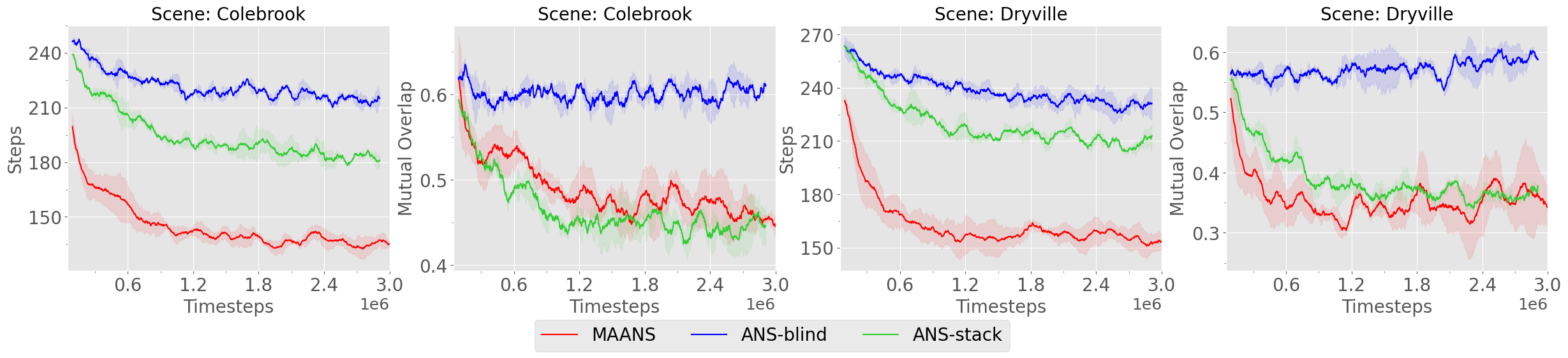
We report the training performances of multiple RL variants on 2 selected scenes, Colebrook and Dryville, and measure the Steps and the Mutual Overlap over these 2 scenes.
5.4.1 Comparison with ANS variants
We first consider 2 ANS variants, ANS-blind and ANS-stack, other than MAANS.
-
•
ANS-blind We train ANS agents to explore blindly, i.e., without any communication, in the environment.
-
•
ANS-stack We directly stack all the agent-centric local maps from the neural SLAM module as the input representation to the global planner, and retrain the ANS global planner under our multi-agent task setting.
We demonstrate the training curves in Fig. 4. Regarding the Steps, both ANS variants perform consistently worse than MAANS on each map. Regarding the Mutual Overlap, the blind variant fails to cooperate completely while the stack variant produces comparable Mutual Overlap to MAANS despite its low exploration efficiency. We remark that ANS-stack performs global and local planning completely on the agent-centric local map while the local map is a narrow sub-region over the entire house, which naturally leads to a much conservative exploration strategy and accordingly helps produces a lower Mutual Overlap.
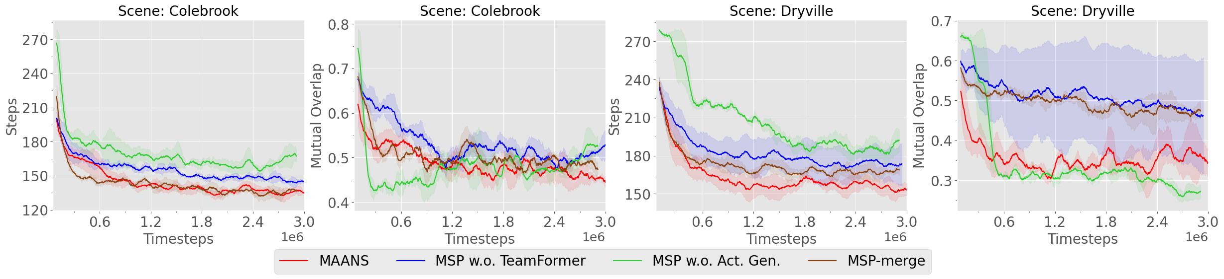
5.4.2 Ablation Study on MSP
We consider 3 additional MSP variants:
-
•
MSP w.o. TeamFormer: We completely substitute Spatial-TeamFormer with a simple average pooling layer over the extracted spatial features from CNN extractors.
-
•
MSP w.o. Act. Gen. We remove the region head from the spatial action generator, so that the global goal is directly generated over the entire refined global map via two Gaussian action distributions. We remark that such an action space design follows the original ANS paper (Savinov et al., 2019).
-
•
MSP-merge We consider another MSP variant that applies a single CNN feature extractor over the manually merged global map from the map merger, instead of forcing the network to learn to fuse each agent’s information.
As shown in Fig. 5, the full MAANS module produces the lowest Steps and Mutual Overlap. Among all the MSP variants, MSP w.o. Act. Gen. produces the highest Steps. This suggests that a simple Gaussian representation of actions may not be able to fully capture the distribution of good long-term goals, which can be highly multi-modal in the early exploration stage. In scene Dryville, MSP w.o. TeamFormer performs much worse and shows larger training unstability than the full model, showing the importance of jointly leveraging intra-agent and spatial relationships in a hierarchical manner. In addition, MSP-merge produces a very high Mutual Overlap in scene Dryville. We hypothesis that this is due to the fact that many agent-specific information are lost in the manually merged maps while MSP can learn to utilize these features implicitly.
5.4.3 Ablation Study on Spatial-TeamFormer
We consider the following variants of MAANS by altering the components of Spatial-TeamFormer as follows:
-
•
No Ind. Spatial Enc.: Individual Spatial Encoder is removed from Spatial-TeamFormer
-
•
No Team Rel. Enc.: Similarly, this variant removes Team Relation Encoder while only keeps Individual Spatial Encoder.
-
•
Unified: This variant applies a single unified transformer over the spatial features from all the agents instead of the hierarchical design in Spatial-TeamFormer. In particular, we directly feed all the features into a big transformer model to generate an invariant representation.
-
•
Flattened: In this variant, we do not keep the spatial structure of feature maps. Instead, we first convert the CNN extracted feature into a flatten vector for each agent and then simply feed these flattened vectors to a standard transformer model for feature learning. We remark that this variant is exactly the same as (Wang et al., 2021).
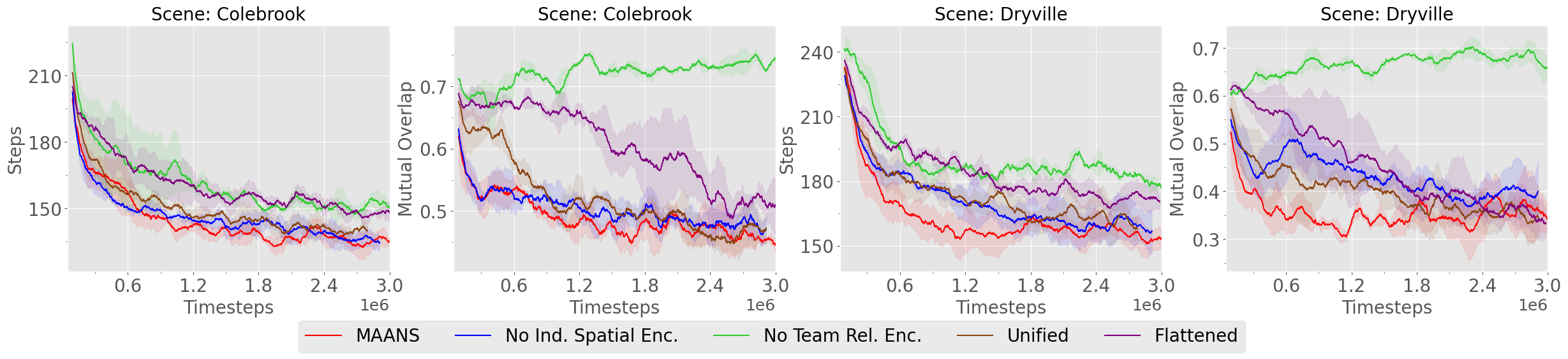
We report training curves in Fig. 6. Compared with Spatial-TeamFormer, No Team Rel. Enc. has the highest Mutual Overlap and worst Steps on both scenes, which suggests that lacking partners’ relationship attention significantly lowers the cooperation efficiency. We remark that No Team Rel. Enc. is indeed a single-agent variant of Spatial-TeamFormer: each agent plans global goal using its individual information while doing path planning still with the merged global map. The variant using Flattened features is also performing much worse than the full model with a clear margin, showing that the network architecture without utilizing spatial inductive bias could hurt final performance. When individual spatial encoder is removed (No Ind. Spatial Enc.), the sample efficiency drops greatly in scene Dryville and the method achieves a higher Mutual Overlap than MAANS. Unified also has worse sample efficiency that the full model. Note that Unified shows greater performance than Flattened, again confirming the importance of utilizing spatial inductive bias.
5.5 Main Results
Due to space constraints, we only present a selected portion of the most competitive results in the main paper and defer the full results to Appendix F.
5.5.1 Comparison with Planning-based Baselines and RL baseline
(1) Training with a Fixed Team Size: We first report the performance of MAANS and selected the baseline methods with a fixed team size of agents on both representative training scenes and testing scenes in Table 1. We remark that only 9 policies of representative training scenes are used to do policy distillation(PD) since it takes a lot of work to train a separated policy for each scene. Except for the Mutual Overlap on the testing scenes where the performance is slightly worse than Voronoi, MAANS still outperforms all planning-based baselines in Steps and Coverage metrics on training and testing scenes. More concretely, MAANS reduces 20.56% exploration steps on training scenes and 7.99% exploration steps on testing scenes than the best planning-based competitor. We also compare with an RL baseline MAANS w.o. PD, which is trained by randomly sampling all training scenes instead of policy distillation. MAANS w.o. PD performs much worse than MAANS on both training and testing scenes, and slightly worse than the best single-agent planning-based method RRT and multi-agent planning-based method Voronoi on testing scenes, indicating the necessity of introducing policy distillation.
We also observe that APF and WMA-RRT, as multi-agent planning baselines, even perform worse than single-agent methods. We empirically found this is due to the formally-designed cooperation paradigm they adopt, which imposes great restriction to agents’ behaviors. In contrast, MAANS, by using MSP, could perform more complicated cooperative strategy to fully explore the scene. Further illustration and analysis could be found in Appendix F.3.
| Sce. | Metrics | Utility | RRT | APF | WMA-RRT | Voronoi | MAANS w.o PD | MAANS |
|---|---|---|---|---|---|---|---|---|
| Train | Mut. Over. | 0.68(0.01) | 0.53(0.02) | 0.61(0.01) | 0.61(0.01) | 0.44(0.01) | 0.46(0.01) | 0.42(0.01) |
| Steps | 236.15(3.61) | 199.59(3.27) | 251.41(3.15) | 268.20(2.24) | 237.04(2.95) | 180.25(2.35) | 158.55(2.25) | |
| Coverage | 0.92(0.01) | 0.96(0.00) | 0.90(0.01) | 0.87(0.01) | 0.93(0.00) | 0.96(0.00) | 0.97(0.00) | |
| Test | Mut. Over. | 0.69(0.01) | 0.57(0.01) | 0.57(0.01) | 0.64(0.01) | 0.51(0.01) | 0.57(0.01) | 0.54(0.02) |
| Steps | 161.28(2.32) | 157.29(2.59) | 181.18(4.17) | 198.92(3.83) | 156.68(3.21) | 159.53(2.73) | 144.16(2.52) | |
| Coverage | 0.95(0.00) | 0.95(0.01) | 0.93(0.01) | 0.91(0.01) | 0.96(0.01) | 0.96(0.00) | 0.96(0.00) |
(2) Zero-Shot Transfer to Different Team Sizes: In this part, we directly apply the policies trained with agents to the scenes of agents respectively. The zero-shot generalization performance of MAANS compared with the best single-agent baseline RRT and the best multi-agent baseline Voronoi on both training and testing scenes is shown in Table 2. Note that experiments on testing scenes are extremely challenging since MAANS is never trained with team sizes on testing scenes. Although MAANS is only trained on the team size of on training scenes, MAANS achieves much better performance than the best planning-based methods with every novel team size on training scenes (17.56% fewer Steps with and 18.36% fewer Steps with ) and comparable performance on testing scenes ( more Steps with ).
| # Agent | Metrics | Training Scenes | Testing Scenes | ||||
| RRT | Voronoi | MAANS | RRT | Voronoi | MAANS | ||
| 3 | Mut. Over. | 0.44(0.01) | 0.37(0.01) | 0.42(0.01) | 0.45(0.01) | 0.43(0.01) | 0.53(0.01) |
| Steps | 155.13(3.26) | 180.27(2.51) | 127.88(1.91) | 128.33(1.66) | 119.98(2.31) | 122.48(2.22) | |
| Coverage | 0.95(0.01) | 0.95(0.00) | 0.97(0.00) | 0.95(0.01) | 0.96(0.00) | 0.96(0.00) | |
| 4 | Mut. Over. | 0.36(0.01) | 0.34(0.01) | 0.42(0.01) | 0.41(0.01) | 0.39(0.01) | 0.50(0.01) |
| Steps | 140.57(1.78) | 147.01(2.38) | 114.75(1.69) | 111.30(1.58) | 101.90(2.36) | 109.07(2.02) | |
| Coverage | 0.92(0.01) | 0.93(0.00) | 0.96(0.00) | 0.93(0.01) | 0.95(0.00) | 0.94(0.00) | |
| 2 3 | Mut. Over. | 0.36(0.01) | 0.35(0.01) | 0.30(0.01) | 0.43(0.01) | 0.32(0.02) | 0.46(0.01) |
| Steps | 185.94(1.83) | 200.91(2.32) |
|
136.42(2.41) | 148.12(6.69) | 134.11(2.88) | |
| Coverage | 0.94(0.00) | 0.92(0.00) | 0.96(0.00) | 0.96(0.01) | 0.92(0.05) | 0.96(0.00) | |
| 3 2 | Mut. Over. | 0.35(0.01) | 0.33(0.01) | 0.41(0.01) | 0.39(0.01) | 0.42(0.01) | 0.43(0.01) |
| Steps | 187.93(1.98) | 206.94(2.50) | 145.14(2.83) | 139.52(3.74) | 133.77(2.83) | 145.43(3.44) | |
| Coverage | 0.91(0.00) | 0.89(0.01) | 0.95(0.00) | 0.94(0.01) | 0.95(0.01) | 0.94(0.01) | |
(3) Varying Team Size within an Episode We further consider the setting where the team size varies within an episode. We summarize the zero-shot generalization performance of MAANS compared with two selected planning-based methods RRT and Voronoi in Table 2. We use "" to denote that each episode starts with agents and the team size immediately switches to after timesteps. Note that MAANS is trained on the training scenes with fixed team size, the varying team size setting is a zero-shot generalization challenge for MAANS. In cases where the team size increases, MAANS produces substantially better performances w.r.t. every metric. In particular, MAANS achieves 33 fewer Steps in training scenes and lower Steps than other methods in testing scenes, which suggests that MAANS has the capability to adaptively adjust its strategy. Regarding the cases where the team size decreases, MAANS consumes over fewer in than RRT in training scenes.
We remark that decreasing the team size is particularly challenging since the absence of some agents might immediately leave a large part of the house unexplored and consequently, the team should immediately update their original plan with drastically different goal assignments.
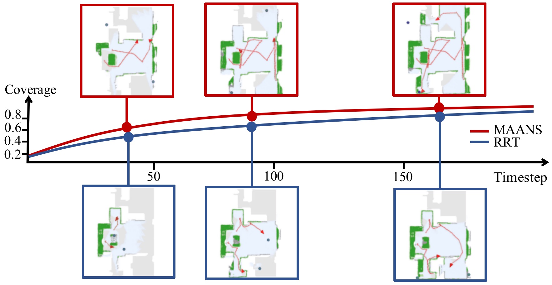
5.6 Learned Strategy
Fig. 7 demonstrates two 2-agent trials of MAANS and RRT, the most competitive planning-based method, with the same birth place. The merged global map are shown in keep timesteps. As shown in Fig 7, MAANS’s coverage ratio goes up faster than RRT, indicating higher exploration efficiency. At timestep around , MAANS produces global goals successfully allocate the agents towards two distant unexplored area while RRT guides the agents towards the same part of the map. And at timestep around when MAANS reaches coverage ratio, RRT still stuck in previous explored area though there is obviously another large open space. Notice that at this key timestep RRT selects two frontiers that are marked unexplored but with no actual benefit, which an agent utilizing prior knowledge about room structures would certainly avoid.
6 Conclusion
We propose the first multi-agent cooperative exploration framework, Multi-Agent Active Neural SLAM (MAANS) that outperforms planning-based competitors in a photo-realist physical environment. The key component of MAANS is the RL-based planning module, Multi-agent Spatial Planner (MSP), which leverages a transformer-based architecture, Spatial-TeamFormer, to capture team-size-invariant representation with strong spatial structures. We also implement a collection of multi-agent-specific enhancements and policy distillation for better generalization. Experiments on Habitat show that MAANS achieves better training and testing performances than all the baselines. We hope MAANS can inspire more powerful multi-agent methods in the future.
We would suggest to visit https://sites.google.com/view/maans for more information.
Appendix A MAANS Details
Multi-Agent Active Neural SLAM (MAANS) consists of 4 modules (1) Neural SLAM; (2) Map Refiner and Map Merger; (3) Local Policy and Local Planner; (4) Multi-agent Spatial Planner (MSP). Here we describe each module in detail.
A.1 Neural SLAM
The Neural SLAM Module for map reconstruction and pose estimation and the Local Policy for action output in our work are directly derived from ANS (Chaplot et al., 2020a). Neural SLAM Module trained by supervised learning provides each agent an updated reconstructed map individually at every timestep. In order to recover a metric map with high accuracy, Neural SLAM Module takes as input current RGB observation , current and last pose from sensors, last pose estimation and last map prediction , and outputs a map prediction and a pose estimation , where represents the current timestep. Note that noises are introduced in simulation to mimic realistic situations.
A.2 Map Refiner and Map Merger
For a better choice of cooperative global goals, we designed a Map Refiner for arranging all maps into the same coordinate system and a Map Merger for shared map reconstruction. More concretely, Map Refiner obtains the egocentric global map from a series of past egocentric local maps and unifies the global maps from all agents in the same coordinate system based on the pose estimates. Besides, there is a dilemma that the egocentric local map contains part of redundant space if an agent reaches the edge of the house, resulting in a large portion of invisible region around the explorable area. To promise an effective CNN feature extraction and more accurate global goal generation, we clip the unexplorable boundary and enlarge the explorable region.
Map Merger leverages all enlarged global maps from the Map Refiner to compose a shared map through max-pooling operator for each pixel location, which indicates the probability of being explored or the obstacle. As a result, the local planner produces the sub-goals on the merged global map, which is much more informative. Note that the merged map is merely employed in local planner to plan path, but not introduced in MSP, which only utilizes agents’ egocentric global maps to infer global goals.
A.3 Local Planner and Local Policy
To effectively reach a global goal, the agent first plans a path to this long-term goal in a manually merged global map using Local Planner, which is mainly based on Fast Marching Method (FMM) (Sethian, 1996), and generates a sequence of short-term sub-goals. The Local Policy learns to produce next action via imitation learning. The input of the Local Policy includes the relative angle and distance from the current position to the short-term goal as well as current RGB observations.
A.4 Multi-agent Spatial Planner
A.4.1 Input Representation
The shared CNN Feature Extractor in Multi-agent Spatial Planner firstly takes in a map with 6 channels as input, containing
-
•
Obstacle channel: indicating the likelihood of being an obstacle of each pixel
-
•
Explored region channel: denoting the probability of being explored of each pixel
-
•
One-hot position channel: describing the position of the agent with an one-hot metric map.
-
•
Trajectory channel: expressing the history trace of each agent with exponentially decaying weight to emphasize the direction of the trace:
where denotes the trajectory channel at timestep .
-
•
One-hot global goal channel: demonstrating the position of the last global goal in an one-hot manner.
-
•
One-hot Goal history channel: recording all the previous global goals of the agent.
Besides CNN spatial maps, we also introduce additional features, including agent-specific embeddings of its identity and current position and grid features, i.e., the embeddings of the relative coordinate of each grid to the agent position as well as the embedding of the previous global goal.
-
•
Position Embedding: described as trainable parameters as part of the neural network. Two types of position embeddings are used to distinguish from the decision-making agent and it’s partners. Note that and is respectively 8 and 128.
-
•
Relative Coordinate Embedding: describing the relative position of the agent with the coarse-grained maps.
-
•
Previous Global Goal Embedding: expressing the relative position of last global goal with the coarse-grained maps.
These embeddings are all concatenated with features outputted by CNN feature extractors and then fed into MSP.
A.4.2 Hierarchical Action Space
MAANS adopts a hierarchical action space to represent global goals, where a global goal is consequently composed of a high-level discrete region and a low-level fine-grained continuous point . To be more specific, the whole world-frame occupancy map is discretized into uniform regions and a global goal is decomposed into two levels,
In MSP, the region head outputs a 64-dim vector denoting the categorical distribution of , while the point head outputs a bivariate Gaussian distribution . Point is obtained by applying Sigmoid to the Gaussian random variables, i.e.,
A.4.3 Reward Function
We design the reward in a team-based fashion, comprising of the coverage reward, the success reward, the overlap penalty and the time penalty. For a unified representation, indicates the total coverage ratio at timestep , is the the total coverage area at timestep , and represents the explored area of agent . The details of 4 kinds of reward gained by agent at timestep are listed as below.
-
•
Coverage Reward: The coverage reward is a combination of the team coverage reward and the individual coverage reward. Team coverage reward illustrates the increment of explored area at timestep , and is proportional to . For the consideration of individual contribution to the whole team exploration, the individual coverage reward is proportional to . We remark that , which suppresses cooperation but leads to the individual exploration. The coefficient is .
-
•
Success Reward: To encourage agent achieves the target coverage ratio as much as possible, we give the bonus to the agent if the total coverage rate is reached in , and when coverage rate is realized.
-
•
Overlap Penalty: The overlap penalty is applied to reduce repetitive exploration among agents so as to enhance cooperation capability. It is described as:
denotes the increment of the average overlapped explored area between each two agents at timestep . In practical, the between agent and agent transforms into the sum of a one-hot map, where the grid on the map will be valued when its total value of two agents’ explored probability is greater than .
-
•
Time Penalty: For the sake of an efficient exploration, we propose the time penalty:
The linear combination of four parts is the final team-based reward. Note that all the explored and obstacle maps are in the scale of for each grid and the measurement unit of all the area is .
A.4.4 Architecture
CNN feature extractor is composed of 5 convolution layers as well as max pooling layers. Hyperparameters of these layers are listed in Table 3. Except the last layer, each layer is followed by a max pooling layer with kernel size .
The core part of MSP, Spatial-Teamformer, contains several blocks, each of which consists of two layers, i.e. an Individual Spatial Encoder and a Team Relation Encoder. Both Individual Spatial Encoder and Team Relation Encoder are self-attention layers with residual connection. We remark that the self-attention mechanism in MSP is exactly the same as transformer encoder in (Dosovitskiy et al., 2020). Hyperparameters of Spatial-Teamformer are listed in Table 4.
| Layer | Out Channels | Kernel Size | Stride | Padding |
| 1 | 32 | 3 | 1 | 1 |
| 2 | 64 | 3 | 1 | 1 |
| 3 | 128 | 3 | 1 | 1 |
| 4 | 64 | 3 | 1 | 1 |
| 5 | 32 | 3 | 2 | 1 |
| hyperparameters | value |
|---|---|
| # of attention heads | 4 |
| attention head dimension | 32 |
| attention hidden Size | 128 |
| # of Spatial-Teamformer blocks | 2 |
Appendix B Baselines
We implemented 6 classical planning-based methods, including 3 single-agent methods and 3 multi-agent baselines.
B.1 Single-agent Baselines
- •
- •
-
•
RRT (Umari & Mukhopadhyay, 2017) generates a collision-free random tree rooted at the agent’s current location. After collecting enough tree nodes that lie on unexplored region, i.e. frontiers, RRT chooses the one with the highest utility , where and are respectively the normalized information gain and navigation cost of . Pseudocode of RRT is shown in Algorithm 1. In each iteration, a random point is draw and a new node is generated by expanding from to with distance , where is the closest tree node to . If segment has no collision with obstacles in , is inserted into the target list or the tree according to whether is in unexplored area or not. Finally, the goal is chosen from the target list with the largest utility where is the information gain and is the navigation cost. is computed by the number of unexplored grids within to , as mentioned above. is computed as the euclidean distance between the agent location and point . To keep these two values at the same scale, we normalize and to w.r.t all cluster centers.
B.2 Multi-agent Baselines
-
•
APF (Yu et al., 2021b) first computes a potential field based on explored occupancy map and current agent locations, and then follows the fastest descending direction of to find a frontier as the global goal. Resistance force among agents is introduced in APF to avoid repetitive exploration. Pseudocode of APF is provided in Algorithm 2. Line 6-12 computes the resistance force between every pair of agents where is the influence radius. In line 13-18, distance maps starting from cluster centers are computed and the corresponding reciprocals are added into the potential field so as one agent approaches the frontier, the potential drops. Here is the weight of cluster , which is the number of targets in this cluster. Consequently an agent would prefer to seek for frontiers that are closer and with more neighboring frontiers. Line 20-25 shows the process to find the fastest potential descending path, at each iteration the agent moves to the cell with the smallest potential among all neighboring ones. is the maximum number of iterations and is repeat penalty to avoid agents wandering around cells with same potentials.
-
•
WMA-RRT (Nazif et al., 2010) WMA-RRT is a multi-agent variant of RRT. Pseudocode of WMA-RRT is provided in Algorithm 3. By maintaining a rooted tree together, agents share information to finish exploration. To impose cooperation using the shared tree, WMA-RRT uses a locking mechanism to avoid agents exploring same part of the tree and restricts agents to walking along the edge of the tree to ensure a strict system. Agents choose a node in the tree as a global goal and mark whether a subtree has been completedly searched. Although this is a multi-agent variant of RRT, we empirically found it perform much worse than RRT. We found this is because the locking mechanism actually restricts agent behaviors greatly and the algorithm itself is incompatible with active SLAM. For the former, agents are often forced not to explore large open areas which require multi-agent effort because locked by another agent. For the latter, WMA-RRT was originally designed for the case a ground-truth mapping is given and adding new nodes into the tree during exploration would cause mis-labeled completed subtree. Also, WMA-RRT do not perform value estimation over the nodes, making agents committed to branches that do not increase coverage much. Therefore, though WMA-RRT is guaranteed to reach fully coverage, it’s inherently not suitable for the setting to maximize coverage ratio. As a comparison between RRT and WMA-RRT, WMA-RRT only utilizes RRT to expand tree while perform multi-agent planning using a strict tree-search procedure while RRT uses the random tree equipped with utility estimation to do planning. For detailed description of the algorithm, we encourage readers to check out (Nazif et al., 2010).
-
•
Voronoi (Hu et al., 2020) The voronoi-based method first partitions the map via voronoi partition and assigns components to agents so that each agent owns parts that are closest to it. Then each agent finds its own global goal by finding a frontier point with largest potential as in Utility within its own partition. In this way, duplicated exploration is be avoided. Pseudocode of Voronoi is provided in Algorithm 4.
Finally, we also evaluate the performance of random policies for references. To eliminate negative impact of visual blind area, the area within a distance of to the agent is virtually marked as explored when choosing frontiers so that these baselines would output far enough global goals. The number of unexplored grids within a distance of to a frontier is defined as the information gain. All these baselines regenerate new global goals every time steps, which is consistent with MSP. Case studies and failure modes of these methods are provided in Section F.3.
Appendix C Evaluation Metrics
We select 3 behavior statistics metric to show different characteristics of particular exploration methods.
-
•
Coverage: Coverage represents the ratio of areas explored by the agents to the entire explorable space in the indoor scene at the end of the episode. Higher Coverage implies more effective exploration. A cell of is considered explored/covered when the 2D projection on the floor of some depth image in the exploration history covers this cell.
-
•
Steps: Steps is the number of timesteps used by agents to achieve a coverage ratio of within an episode. Fewer Steps implies faster exploration.
-
•
Mutual Overlap: For effective collaboration, each agent should visit regions different from those explored by its teammates. We measure the average overlapping explored area over each pair of agents when the coverage ratio reaches 90%, which we call Mutual Overlap. Mutual Overlap denotes the normalized value of mutual overlap. Lower Mutual Overlap suggests better multi-agent coordination.
Appendix D Training Details
We adopt Multi-Agent Proximal Policy Optimization (MAPPO) (Yu et al., 2021a), a multi-agent extension of PPO, to train MSP. The pseudocode of MAPPO is provided in Algorithm 5. Detailed hyper-parameters are listed in Table 5.
| common hyperparameters | value |
|---|---|
| gradient clip norm | 10.0 |
| GAE lambda | 0.95 |
| gamma | 0.99 |
| value loss | huber loss |
| huber delta | 10.0 |
| mini batch size | batch size / mini-batch |
| optimizer | Adam |
| optimizer epsilon | 1e-5 |
| weight decay | 0 |
| network initialization | Orthogonal |
| use reward normalization | True |
| use feature normalization | True |
| learning rate | 2.5e-5 |
| parallel environment threads | 10 |
| number of local steps | 15 |
As for policy distillation, an expert network is trained, where is the region head, is the point head, is the state, for each training scenes and team size of . After that, a student network is trained via performing behavior cloning from these expert networks. The student network is trained in dagger style: for each episode, we first collect data using , and then run several updates to optimize the output of student using past experience. The objective function to minimize is sum of , which is the KL divergence between the student region distribution and teacher region distribution , and , which is the square error loss between point head of student and that of teacher. Policy distillation uses Adam optimizer with learning rate.
Appendix E Experimental Setting
E.1 Datasets
We follow the dataset used in Active Neural SLAM (ANS) (Chaplot et al., 2020a). The original Gibson Challenge dataset (Xia et al., 2018a), which could be used with Habitat Simulator, provides training and validation scenes. Note that Gibson testing set is not public but rather held on an online evaluation server for the PointGoal task, so the validation set is used as the testing instead of hyper-parameter tuning. We have made substantial efforts to check every single scene from the Gibson Challenge dataset and have to exclude a large portion of scenes not suitable for multi-agent exploration, including (i) scenes that have large disconnected regions; and (ii) scenes that have multiple floors (agents can not go upstairs) so that the agents are not possible to reach 90% coverage of the entire house. Note that disconnected region is not an issue for semantic or point navigation tasks.
We categorize the remaining scenes into training scenes, including 9 small scenes, 9 middle scenes and 5 large scenes based on explorable area, as well as testing scenes, which including 5 small scenes, 4 middle scenes and 1 large scene. Note that the validation set of the original Gibson Challenge dataset, i.e. the testing set, has 14 scenes, of which 8 scenes are eligible for our task, including 5 small scenes, 1 middle scene and 1 large scene. Since most scenes in the testing set are too small for multi-agent exploration task, we additionally add 3 middle scenes to the testing set. The common training paradigm for visual exploration is to randomly sample training scenes or team sizes at each training episode (Chen et al., 2019). However, we empirically observe that different Habitat scenes and team sizes may lead to drastically different exploration difficulties. During training, gradients from different configurations may negatively impact each other. Hence, our solution is to train a separate policy on each map and use policy distillation to extract a meta policy to tackle this problem.
E.2 Assumption of Birth Position
We assume the agents has access to the birth location of each other while the locations during an episode are estimated using Neural SLAM module. The merged global map is fused using the estimated locations and the birth place.
E.3 Episode Length
First, we empirically found that as the number of agents grows, even random exploration can be particularly competitive (as shown in Table 8), which, we believe, is due to the limited explorable space of Gibson scenes. Hence, we only test up to 4 agents and argue that the -agent case is the most challenging. Regarding the episode length, it is estimated according to the number of timesteps when the strongest single-agent planning-based method, RRT, achieves 95% coverage. Note that if the horizon is too long (e.g., 1000, which is used in ANS), almost all the methods will have the same the final coverage rate. In addition, the Mutual Overlap and Steps metrics are all estimated before the agents reach a 90% coverage, which do not depend on the episode length. The choice of a higher re-planning frequency (e.g., re-plan per 15 timestep) is also due to a shorter episode horizon111All the agents will re-generate their personal long-term global goals using MSP in a synchronous manner every timesteps while ANS (Chaplot et al., 2020a) re-plans every 25 timesteps.. All the baselines use the same planning frequency.
Appendix F Additional Experiment Results
F.1 Fixed Team Size
F.1.1 Trained with Team size = 2
We first report the performance of MAANS and all baseline methods with a fixed team size of agents on both 9 representative training scenes and unseen testing scenes in Table 6 and Table 7. MAANS outperforms all the planning-based baselines with a clear margin in every evaluation metric, particularly the Steps, on both training and testing scenes. We can observe that Steps of testing scenes is overall fewer than training scenes since we use 9 middle scenes for training while the testing set has more small scenes. And as the scene size grows, the performance of planning-based methods degrades a lot. We directly apply the policies trained with agents to the scenes of agents respectively. The zero-shot generalization performance of MAANS compared with all the baselines on 9 representative training scenes and testing scenes is shown in Table 8 and Table 9. We can observe that MAANS still outperforms planning-based methods on training scenes. And MAANS could even achieve comparable performance on testing scenes despite MAANS having neither seen the testing scenes nor the novel team sizes.
| Sce. | Metrics | Random | Nearest | Utility | RRT | MAANS |
|---|---|---|---|---|---|---|
| Training Sce. | Mut. Over. | 0.66(0.01) | 0.53(0.02) | 0.68(0.01) | 0.53(0.02) | 0.42(0.01) |
| Steps | 273.56(1.38) | 246.79(3.90) | 236.15(3.61) | 199.59(3.27) | 158.55(2.25) | |
| Coverage | 0.86(0.00) | 0.91(0.01) | 0.92(0.01) | 0.96(0.00) | 0.97(0.00) | |
| Testing Sce. | Mut. Over. | 0.66(0.02) | 0.58(0.01) | 0.69(0.01) | 0.57(0.02) | 0.54(0.02) |
| Steps | 193.83(2.80) | 166.23(3.96) | 161.28(2.32) | 157.29(2.59) | 144.16(2.52) | |
| Coverage | 0.93(0.00) | 0.95(0.00) | 0.95(0.00) | 0.95(0.01) | 0.96(0.00) |
| Sce. | Metrics | Random | APF | WMA-RRT | Voronoi. | MAANS |
|---|---|---|---|---|---|---|
| Training Sce. | Mut. Over. | 0.66(0.01) | 0.61(0.01) | 0.61(0.01) | 0.44(0.01) | 0.42(0.01) |
| Steps | 273.56(1.38) | 251.41(3.15) | 268.20(2.24) | 237.04(2.95) | 158.55(2.25) | |
| Coverage | 0.86(0.00) | 0.90(0.01) | 0.87(0.01) | 0.93(0.00) | 0.97(0.00) | |
| Testing Sce. | Mut. Over. | 0.66(0.02) | 0.57(0.01) | 0.64(0.01) | 0.51(0.01) | 0.54(0.02) |
| Steps | 193.83(2.80) | 181.18(4.17) | 198.92(3.83) | 156.68(3.21) | 144.16(2.52) | |
| Coverage | 0.93(0.00) | 0.93(0.01) | 0.91(0.01) | 0.96(0.01) | 0.96(0.00) |
| # Agent | Metrics | Random | Nearest | Utility | RRT | MAANS |
|---|---|---|---|---|---|---|
| Training Scenes | ||||||
| 3 | Mut. Over. | 0.54(0.01) | 0.46(0.01) | 0.58(0.00) | 0.44(0.01) | 0.42(0.01) |
| Steps | 221.29(1.80) | 188.58(2.02) | 180.82(2.25) | 155.13(3.26) | 127.88(1.91) | |
| Coverage | 0.82(0.01) | 0.91(0.00) | 0.94(0.00) | 0.95(0.01) | 0.97(0.00) | |
| 4 | Mut. Over. | 0.49(0.01) | 0.43(0.01) | 0.52(0.01) | 0.36(0.01) | 0.42(0.01) |
| Steps | 163.11(0.77) | 154.75(2.16) | 151.30(3.03) | 140.57(1.78) | 114.75(1.69) | |
| Coverage | 0.87(0.00) | 0.88(0.01) | 0.91(0.01) | 0.92(0.01) | 0.96(0.00) | |
| Testing Scenes | ||||||
| 3 | Mut. Over. | 0.55(0.01) | 0.51(0.01) | 0.59(0.01) | 0.45(0.01) | 0.53(0.01) |
| Steps | 145.90(2.80) | 131.04(3.53) | 128.46(3.04) | 128.33(1.66) | 122.48(2.22) | |
| Coverage | 0.94(0.00) | 0.95(0.00) | 0.96(0.00) | 0.95(0.01) | 0.96(0.00) | |
| 4 | Mut. Over. | 0.48(0.01) | 0.46(0.01) | 0.54(0.01) | 0.41(0.01) | 0.50(0.01) |
| Steps | 116.94(1.61) | 108.23(1.24) | 110.14(1.93) | 111.30(1.58) | 109.07(2.02) | |
| Coverage | 0.93(0.01) | 0.94(0.00) | 0.94(0.01) | 0.93(0.01) | 0.94(0.00) | |
| # Agent | Metrics | Random | APF | WMA-RRT | Voronoi | MAANS |
|---|---|---|---|---|---|---|
| Training Scenes | ||||||
| 3 | Mut. Over. | 0.54(0.01) | 0.45(0.01) | 0.54(0.01) | 0.37(0.01) | 0.42(0.01) |
| Steps | 221.29(1.80) | 207.20(2.41) | 210.01(2.68) | 180.27(2.51) | 127.88(1.91) | |
| Coverage | 0.82(0.01) | 0.87(0.01) | 0.87(0.01) | 0.95(0.00) | 0.97(0.00) | |
| 4 | Mut. Over. | 0.49(0.01) | 0.35(0.01) | 0.49(0.01) | 0.34(0.01) | 0.42(0.01) |
| Steps | 163.11(0.77) | 170.59(1.06) | 168.07(1.41) | 147.01(2.38) | 114.75(1.69) | |
| Coverage | 0.87(0.00) | 0.79(0.01) | 0.82(0.01) | 0.93(0.00) | 0.96(0.00) | |
| Testing Scenes | ||||||
| 3 | Mut. Over. | 0.55(0.01) | 0.40(0.01) | 0.56(0.01) | 0.43(0.01) | 0.53(0.01) |
| Steps | 145.90(2.80) | 152.62(3.71) | 161.59(3.60) | 119.98(2.31) | 122.48(2.22) | |
| Coverage | 0.94(0.00) | 0.92(0.01) | 0.89(0.02) | 0.96(0.00) | 0.96(0.00) | |
| 4 | Mut. Over. | 0.48(0.01) | 0.30(0.01) | 0.52(0.01) | 0.39(0.01) | 0.50(0.01) |
| Steps | 116.94(1.61) | 133.68(1.35) | 136.88(3.08) | 101.90(2.36) | 109.07(2.02) | |
| Coverage | 0.93(0.01) | 0.88(0.01) | 0.84(0.02) | 0.95(0.00) | 0.94(0.00) | |
F.1.2 Trained with Team size = 3
Here we additionally report the performance of all the baseline methods and MAANS trained with a fixed team size of agents on 9 representative training scenes and testing scenes in Table 10 and Table 11. Except for comparable performance to Voronoi on testing scenes, MAANS consistently outperforms other planning-based baselines in all metrics on both training scenes and testing scenes. When training with team size , MAANS also exhibits surprising zero-shot transfer ability to various team sizes on training and testing scenes as shown in Table 12 and Table 13. More concretely, MAANS trained with a fixed team size shows much better performance than all planning-based methods on training scenes and comparable performance on testing scenes. Besides, we can observe that MAANS trained with a fixed team size and MAANS trained with a fixed team size are better than each other with corresponding training team size. MAANS trained with a fixed team size performs better in 4-agent case, showing less and fewer on training scenes and less and fewer on testing scenes.
| Sce. | Metrics | Random | Nearest | Utility | RRT | MAANS |
|---|---|---|---|---|---|---|
| Training Sce. | Mut. Over. | 0.54(0.01) | 0.46(0.01) | 0.58(0.00) | 0.44(0.01) | 0.33(0.01) |
| Steps | 221.29(1.80) | 188.58(2.02) | 180.82(2.25) | 155.13(3.26) | 121.99(1.91) | |
| Coverage | 0.82(0.01) | 0.91(0.00) | 0.94(0.00) | 0.95(0.01) | 0.97(0.00) | |
| Testing Sce. | Mut. Over. | 0.55(0.01) | 0.51(0.01) | 0.59(0.01) | 0.45(0.01) | 0.48(0.01) |
| Steps | 145.90(2.80) | 131.04(3.53) | 128.46(3.04) | 128.33(1.66) | 121.62(1.96) | |
| Coverage | 0.94(0.00) | 0.95(0.00) | 0.96(0.00) | 0.95(0.01) | 0.96(0.00) |
| Sce. | Metrics | Random | APF | WMA-RRT | Voronoi | MAANS |
|---|---|---|---|---|---|---|
| Training Sce. | Mut. Over. | 0.54(0.01) | 0.45(0.01) | 0.54(0.01) | 0.37(0.01) | 0.33(0.01) |
| Steps | 221.29(1.80) | 207.20(2.41) | 210.01(2.68)) | 180.27(2.51) | 121.99(1.91) | |
| Coverage | 0.82(0.01) | 0.87(0.01) | 0.87(0.01) | 0.95(0.00) | 0.97(0.00) | |
| Testing Sce. | Mut. Over. | 0.55(0.01) | 0.40(0.01) | 0.56(0.01) | 0.43(0.01) | 0.48(0.01) |
| Steps | 145.90(2.80) | 152.62(3.71) | 161.59(3.60) | 119.98(2.31) | 121.62(1.96) | |
| Coverage | 0.94(0.00) | 0.92(0.01) | 0.89(0.02) | 0.96(0.00) | 0.96(0.00) |
| # Agent | Metrics | Random | Nearest | Utility | RRT | MAANS |
|---|---|---|---|---|---|---|
| Training Scenes | ||||||
| 2 | Mut. Over. | 0.66(0.01) | 0.53(0.02) | 0.68(0.01) | 0.53(0.02) | 0.33(0.01) |
| Steps | 273.56(1.38) | 246.79(3.90) | 236.15(3.61) | 199.59(3.27) | 167.24(2.12) | |
| Coverage | 0.86(0.00) | 0.91(0.01) | 0.92(0.01) | 0.96(0.00) | 0.96(0.00) | |
| 4 | Mut. Over. | 0.49(0.01) | 0.43(0.01) | 0.52(0.01) | 0.36(0.01) | 0.34(0.01) |
| Steps | 163.11(0.77) | 154.75(2.16) | 151.30(3.03) | 140.57(1.78) | 106.12(2.19) | |
| Coverage | 0.87(0.00) | 0.88(0.01) | 0.91(0.01) | 0.92(0.01) | 0.96(0.00) | |
| Testing Scenes | ||||||
| 2 | Mut. Over. | 0.66(0.02) | 0.58(0.01) | 0.69(0.01) | 0.57(0.02) | 0.52(0.01) |
| Steps | 193.83(2.80) | 166.23(3.96) | 161.28(2.32) | 157.29(2.59) | 154.95(2.95) | |
| Coverage | 0.93(0.00) | 0.95(0.00) | 0.95(0.00) | 0.95(0.01) | 0.96(0.00) | |
| 4 | Mut. Over. | 0.48(0.01) | 0.46(0.01) | 0.54(0.01) | 0.41(0.01) | 0.46(0.01) |
| Steps | 116.94(1.61) | 108.23(1.24) | 110.14(1.93) | 111.30(1.58) | 103.52(1.98) | |
| Coverage | 0.93(0.01) | 0.94(0.00) | 0.94(0.01) | 0.93(0.01) | 0.95(0.00) | |
| # Agent | Metrics | Random | APF | WMA-RRT | Voronoi | MAANS |
|---|---|---|---|---|---|---|
| Training Scenes | ||||||
| 2 | Mut. Over. | 0.66(0.01) | 0.61(0.01) | 0.61(0.01) | 0.44(0.01) | 0.33(0.01) |
| Steps | 273.56(1.38) | 251.41(3.15) | 268.20(2.24) | 237.04(2.95) | 167.24(2.12) | |
| Coverage | 0.86(0.00) | 0.90(0.01) | 0.87(0.01) | 0.93(0.00) | 0.96(0.00) | |
| 4 | Mut. Over. | 0.49(0.01) | 0.35(0.01) | 0.49(0.01) | 0.34(0.01) | 0.34(0.01) |
| Steps | 163.11(0.77) | 170.59(1.06) | 168.07(1.41) | 147.01(2.38) | 106.12(2.19) | |
| Coverage | 0.87(0.00) | 0.79(0.01) | 0.82(0.01) | 0.93(0.00) | 0.96(0.00) | |
| Testing Scenes | ||||||
| 2 | Mut. Over. | 0.66(0.02) | 0.57(0.01) | 0.64(0.01) | 0.51(0.02) | 0.52(0.01) |
| Steps | 193.83(2.80) | 181.18(4.17) | 198.92(3.83) | 156.68(3.21) | 154.95(2.95) | |
| Coverage | 0.93(0.00) | 0.93(0.01) | 0.91(0.01) | 0.96(0.01) | 0.96(0.00) | |
| 4 | Mut. Over. | 0.48(0.01) | 0.30(0.01) | 0.52(0.01) | 0.39(0.01) | 0.46(0.01) |
| Steps | 116.94(1.61) | 133.68(1.35) | 136.88(3.08) | 101.90(2.36) | 103.52(1.98) | |
| Coverage | 0.93(0.01) | 0.88(0.01) | 0.84(0.02) | 0.95(0.00) | 0.95(0.00) | |
F.2 Varying Team Size
We further consider the setting where the team size varies within an episode. We summarize the zero-shot generalization performance of MAANS compared with the planning-based baselines on training scenes in Table 14 and Table 15. We use "" to denote that each episode starts with agents and the team size immediately switches to after timesteps. More concretely, in an episode, max(, ) agents are set in the beginning, and - agents are unable to move until timesteps 90 reaches in the increased team size scenarios. The setting is reversed in the decreased ones. We remark that MAANS trained by fixed team size or is separately presented in experiments, which is called MAANS(N=2) or MAANS(N=3).
In scenarios where the team size increases, though RRT still performs the best among the planning-based baselines, MAANS outperforms RRT with a clear margin for fewer in setting and fewer in others. While as the team size decreases, the performance between MAANS and classical methods varies more widely, which shows that MAANS has a fewer in the comparison of the best baseline, RRT. Besides, MAANS has the best result in the metrics of mutual overlap ratio and coverage. We consider the case is more challenging where the team size decreases and the share information gain becomes less shapely, therefore the baselines could not adjust the strategy immediately.
| # Agent | Metrics | Random | Nearest | Utility | RRT |
|
|
||||
|---|---|---|---|---|---|---|---|---|---|---|---|
| Increase Number of Agents | |||||||||||
| Mut. Over. | 0.54(0.01) | 0.43(0.01) | 0.56(0.01) | 0.36(0.01) | 0.30(0.01) | 0.25(0.01) | |||||
| Steps | 223.63(2.16) | 211.73(1.96) | 210.88(1.30) | 185.94(1.83) | 148.82(2.01) | 146.34(1.76) | |||||
| Coverage | 0.86(0.01) | 0.89(0.01) | 0.90(0.00) | 0.94(0.00) | 0.96(0.00) | 0.96(0.00) | |||||
| Mut. Over. | 0.42(0.01) | 0.37(0.01) | 0.47(0.00) | 0.31(0.01) | 0.26(0.01) | 0.22(0.01) | |||||
| Steps | 175.89(0.64) | 174.06(0.72) | 174.55(0.69) | 165.43(0.97) | 142.96(1.24) | 138.22(1.36) | |||||
| Coverage | 0.82(0.01) | 0.81(0.01) | 0.81(0.00) | 0.88(0.01) | 0.94(0.00) | 0.94(0.00) | |||||
| Mut. Over. | 0.45(0.01) | 0.38(0.01) | 0.49(0.01) | 0.26(0.01) | 0.29(0.01) | 0.24(0.01) | |||||
| Steps | 170.90(1.19) | 165.85(0.80) | 165.82(0.72) | 155.15(2.18) | 125.26(1.46) | 119.03(1.36) | |||||
| Coverage | 0.85(0.01) | 0.85(0.00) | 0.87(0.01) | 0.90(0.01) | 0.95(0.00) | 0.96(0.00) | |||||
| Decrease Number of Agents | |||||||||||
| Mut. Over. | 0.48(0.01) | 0.39(0.01) | 0.48(0.01) | 0.35(0.01) | 0.41(0.01) | 0.33(0.01) | |||||
| Steps | 225.51(2.57) | 213.16(1.65) | 209.87(1.75) | 187.93(1.98) | 145.14(2.83) | 142.09(1.98) | |||||
| Coverage | 0.84(0.01) | 0.86(0.01) | 0.88(0.00) | 0.91(0.00) | 0.95(0.00) | 0.95(0.00) | |||||
| Mut. Over. | 0.41(0.01) | 0.36(0.01) | 0.42(0.01) | 0.32(0.01) | 0.40(0.01) | 0.33(0.01) | |||||
| Steps | 173.36(1.08) | 168.89(1.12) | 167.54(1.30) | 157.40(2.56) | 127.35(2.08) | 118.93(2.30) | |||||
| Coverage | 0.81(0.00) | 0.82(0.01) | 0.83(0.01) | 0.86(0.01) | 0.93(0.00) | 0.93(0.00) | |||||
| Mut. Over. | 0.44(0.01) | 0.39(0.01) | 0.47(0.00) | 0.33(0.01) | 0.41(0.01) | 0.33(0.01) | |||||
| Steps | 168.32(1.24) | 161.87(1.08) | 159.96(1.48) | 147.61(1.78) | 119.59(2.31) | 111.24(1.54) | |||||
| Coverage | 0.85(0.00) | 0.85(0.00) | 0.88(0.01) | 0.90(0.01) | 0.95(0.00) | 0.95(0.00) | |||||
| # Agent | Metrics | Random | APF | WMA-RRT | Voronoi |
|
|
||||
|---|---|---|---|---|---|---|---|---|---|---|---|
| Increase Number of Agents | |||||||||||
| Mut. Over. | 0.54(0.01) | 0.42(0.00) | 0.49(0.00) | 0.35(0.01) | 0.30(0.01) | 0.25(0.01) | |||||
| Steps | 223.63(2.16) | 225.35(0.97) | 221.85(0.00) | 200.91(2.32) | 148.82(2.01) | 146.34(1.76) | |||||
| Coverage | 0.86(0.01) | 0.82(0.01) | 0.85(0.00) | 0.92(0.00) | 0.96(0.00) | 0.96(0.00) | |||||
| Mut. Over. | 0.42(0.01) | 0.31(0.01) | 0.44(0.01) | 0.30(0.01) | 0.26(0.01) | 0.22(0.01) | |||||
| Steps | 175.89(0.64) | 178.77(0.13) | 178.91(0.33) | 170.50(0.88) | 142.96(1.24) | 138.22(1.36) | |||||
| Coverage | 0.82(0.01) | 0.68(0.01) | 0.67(0.01) | 0.85(0.01) | 0.94(0.00) | 0.94(0.00) | |||||
| Mut. Over. | 0.45(0.01) | 0.32(0.01) | 0.45(0.00) | 0.31(0.01) | 0.29(0.01) | 0.24(0.01) | |||||
| Steps | 170.90(1.19) | 175.35(0.56) | 173.64(0.41) | 159.23(1.50) | 125.26(1.46) | 119.03(1.36) | |||||
| Coverage | 0.85(0.01) | 0.74(0.01) | 0.79(0.00) | 0.90(0.00) | 0.95(0.00) | 0.96(0.00) | |||||
| Decrease Number of Agents | |||||||||||
| Mut. Over. | 0.48(0.01) | 0.38(0.01) | 0.44(0.00) | 0.33(0.01) | 0.41(0.01) | 0.33(0.01) | |||||
| Steps | 225.51(2.57) | 225.51(1.32) | 226.14(0.00) | 206.94(2.50) | 145.14(2.83) | 142.09(1.98) | |||||
| Coverage | 0.84(0.01) | 0.78(0.01) | 0.81(0.00) | 0.89(0.01) | 0.95(0.00) | 0.95(0.00) | |||||
| Mut. Over. | 0.41(0.01) | 0.32(0.01) | 0.40(0.00) | 0.30(0.01) | 0.40(0.01) | 0.33(0.01) | |||||
| Steps | 173.36(1.08) | 176.79(0.65) | 176.38(0.00) | 165.23(2.80) | 127.35(2.08) | 118.93(2.30) | |||||
| Coverage | 0.81(0.00) | 0.68(0.01) | 0.73(0.00) | 0.83(0.01) | 0.93(0.00) | 0.93(0.00) | |||||
| Mut. Over. | 0.44(0.01) | 0.33(0.01) | 0.44(0.00) | 0.32(0.01) | 0.41(0.01) | 0.33(0.01) | |||||
| Steps | 168.32(1.24) | 173.94(0.81) | 171.85(0.00) | 155.65(2.79) | 119.59(2.31) | 111.24(1.54) | |||||
| Coverage | 0.85(0.00) | 0.73(0.01) | 0.78(0.00) | 0.89(0.01) | 0.95(0.00) | 0.95(0.00) | |||||
When we compare MAANS(N=2) with MAANS(N=3), MAANS(N=3) has a comparable performance with a lower ratio to the other. It indicates that training with a fixed team size helps MAANS grasp the capability of cooperation better so that the strategy is more stable and inflexible in a varying team size situation.
| # Agent | Metrics | Random | Nearest | Utility | RRT |
|
|
||||
|---|---|---|---|---|---|---|---|---|---|---|---|
| Increase Number of Agents | |||||||||||
| Mut. Over. | 0.52(0.01) | 0.47(0.01) | 0.55(0.02) | 0.43(0.01) | 0.46(0.01) | 0.41(0.01) | |||||
| Steps | 159.85(3.60) | 144.60(3.45) | 143.14(1.93) | 136.42(2.41) | 134.11(2.88) | 131.96(1.80) | |||||
| Coverage | 0.93(0.01) | 0.95(0.01) | 0.95(0.00) | 0.96(0.01) | 0.96(0.00) | 0.96(0.00) | |||||
| Mut. Over. | 0.43(0.01) | 0.40(0.01) | 0.47(0.01) | 0.38(0.01) | 0.43(0.01) | 0.37(0.01) | |||||
| Steps | 134.57(0.63) | 129.13(1.86) | 126.92(1.67) | 122.42(1.85) | 122.09(1.99) | 116.66(4.51) | |||||
| Coverage | 0.90(0.00) | 0.91(0.01) | 0.92(0.01) | 0.92(0.00) | 0.93(0.01) | 0.93(0.01) | |||||
| Mut. Over. | 0.46(0.01) | 0.42(0.01) | 0.49(0.01) | 0.37(0.01) | 0.45(0.01) | 0.39(0.00) | |||||
| Steps | 125.08(1.35) | 116.96(1.42) | 115.44(3.38) | 119.02(1.32) | 114.84(1.56) | 110.04(0.54) | |||||
| Coverage | 0.92(0.01) | 0.93(0.00) | 0.93(0.01) | 0.92(0.01) | 0.94(0.00) | 0.94(0.00) | |||||
| Decrease Number of Agents | |||||||||||
| Mut. Over. | 0.45(0.01) | 0.41(0.01) | 0.46(0.01) | 0.39(0.01) | 0.43(0.01) | 0.40(0.00) | |||||
| Steps | 167.98(2.06) | 149.41(2.59) | 146.73(3.44) | 139.52(3.74) | 145.43(3.44) | 146.93(2.93) | |||||
| Coverage | 0.91(0.00) | 0.94(0.00) | 0.93(0.01) | 0.94(0.01) | 0.94(0.01) | 0.94(0.00) | |||||
| Mut. Over. | 0.36(0.01) | 0.33(0.01) | 0.37(0.01) | 0.31(0.00) | 0.37(0.01) | 0.34(0.00) | |||||
| Steps | 140.37(1.80) | 128.11(1.72) | 127.40(0.49) | 125.84(0.83) | 129.73(2.73) | 127.30(1.55) | |||||
| Coverage | 0.88(0.01) | 0.90(0.01) | 0.90(0.01) | 0.90(0.00) | 0.90(0.01) | 0.90(0.00) | |||||
| Mut. Over. | 0.43(0.01) | 0.39(0.00) | 0.44(0.01) | 0.35(0.01) | 0.43(0.01) | 0.39(0.01) | |||||
| Steps | 127.46(1.64) | 117.44(0.89) | 114.56(2.28) | 119.70(1.88) | 116.74(1.38) | 112.72(2.13) | |||||
| Coverage | 0.91(0.01) | 0.93(0.00) | 0.93(0.01) | 0.91(0.00) | 0.93(0.01) | 0.93(0.00) | |||||
| # Agent | Metrics | Random | APF | WMA-RRT | Voronoi |
|
|
||||
|---|---|---|---|---|---|---|---|---|---|---|---|
| Increase Number of Agents | |||||||||||
| Mut. Over. | 0.52(0.01) | 0.38(0.02) | 0.44(0.01) | 0.32(0.02) | 0.46(0.01) | 0.41(0.01) | |||||
| Steps | 159.85(3.60) | 167.87(2.85) | 176.89(5.70) | 148.12(6.69) | 134.11(2.88) | 131.96(1.80) | |||||
| Coverage | 0.93(0.01) | 0.89(0.01) | 0.88(0.01) | 0.92(0.05) | 0.96(0.00) | 0.96(0.00) | |||||
| Mut. Over. | 0.43(0.01) | 0.26(0.01) | 0.33(0.01) | 0.24(0.01) | 0.43(0.01) | 0.37(0.01) | |||||
| Steps | 134.57(0.63) | 148.48(1.01) | 157.48(1.50) | 130.49(1.81) | 122.09(1.99) | 116.66(4.51) | |||||
| Coverage | 0.90(0.00) | 0.78(0.01) | 0.69(0.02) | 0.90(0.01) | 0.93(0.01) | 0.93(0.01) | |||||
| Mut. Over. | 0.46(0.01) | 0.28(0.01) | 0.40(0.00) | 0.30(0.00) | 0.45(0.01) | 0.39(0.00) | |||||
| Steps | 125.08(1.35) | 139.82(1.77) | 141.80(1.53) | 114.99(1.04) | 114.84(1.56) | 110.04(0.54) | |||||
| Coverage | 0.92(0.01) | 0.85(0.01) | 0.83(0.01) | 0.94(0.00) | 0.94(0.00) | 0.94(0.00) | |||||
| Decrease Number of Agents | |||||||||||
| Mut. Over. | 0.45(0.01) | 0.33(0.01) | 0.51(0.01) | 0.42(0.01) | 0.43(0.01) | 0.40(0.00) | |||||
| Steps | 167.98(2.06) | 178.43(2.25) | 171.87(2.53) | 133.77(2.83) | 145.43(3.44) | 146.93(2.93) | |||||
| Coverage | 0.91(0.00) | 0.86(0.01) | 0.87(0.01) | 0.95(0.01) | 0.94(0.01) | 0.94(0.00) | |||||
| Mut. Over. | 0.36(0.01) | 0.23(0.00) | 0.47(0.01) | 0.38(0.00) | 0.37(0.01) | 0.34(0.00) | |||||
| Steps | 140.37(1.80) | 151.69(1.60) | 144.66(1.46) | 115.97(1.93) | 129.73(2.73) | 127.30(1.55) | |||||
| Coverage | 0.88(0.01) | 0.78(0.01) | 0.81(0.01) | 0.93(0.00) | 0.90(0.01) | 0.90(0.00) | |||||
| Mut. Over. | 0.43(0.01) | 0.27(0.01) | 0.48(0.00) | 0.39(0.01) | 0.43(0.01) | 0.39(0.01) | |||||
| Steps | 127.46(1.64) | 142.86(2.31) | 140.68(0.17) | 106.92(2.78) | 116.74(1.38) | 112.72(2.13) | |||||
| Coverage | 0.91(0.01) | 0.84(0.01) | 0.82(0.00) | 0.94(0.01) | 0.93(0.01) | 0.93(0.00) | |||||
We summarize the zero-shot generalization performance of MAANS compared with the planning-based baselines on testing scenes in Table 16 and Table 17. In cases where the team size increases, MAANS still produces substantially better performances, especially , which suggests that MAANS has the capability to adaptively adjust its strategy. Regarding the cases where the team size decreases, MAANS shows slightly worse performance than the best single-agent baseline, RRT, and the best multi-agent baseline, Voronoi. We remark that decreasing the team size is particularly challenging since the absence of some agents might immediately leave a large part of the house unexplored and consequently, the team should immediately update their original plan with drastically different goal assignments.
F.3 Case Studies
We implemented several planning-based methods as baselines, including Nearest, Utility, APF, RRT and additionally a voronoi-based method plus a multi-agent variant of RRT, WMA-RRT. While these methods are respectively tested under environments with ideal assumptions, we empirically found some of them do not work well under our setting with realistic perception and noises.
-
•
Sensitive to realistic noise. Nearest, Utility, APF and the voronoi-based method all apply cell-level goal searching. We empirically found that they share a same failure mode, that is, trying to approach a cell that is wrongly estimated as explorable, even when the mapping only has minor cell-level error. The planning-based baseline RRT do not perform cell-level planning but in a geometric way, thus it’s robust to mapping noise.
-
•
Naive estimation of future value. Both Utility and RRT select candidate frontier with highest utility, which is computed as the number of unexplored cells within a small distance. Such estimation of future values is very short-sighted. In contrast, TANS, by using neural network, could perform more complicated inference about utility of exploring one part of the map.
-
•
Strict restriction over robot behaviors. Among the planning-based baselines, both APF and WMA-RRT adopt a formally-designed cooperation system. However their cooperation schemes both imposes great restriction to agents’ behaviors. APF includes resistance force among agents to avoid duplicated exploration. In WMA-RRT, agents share a same tree and follow a locking-and-searching method to do cooperation. However, in cases where it’s better for agents to go through the same place simultaneously, which is pretty common, the resistance force in APF and the locking mechanism in WMA-RRT prevent agents from the optimal strategy. Meanwhile, WMA-RRT restricts agents to follow paths in the shared tree, losing the benefit of accidental coverage brought by random search.
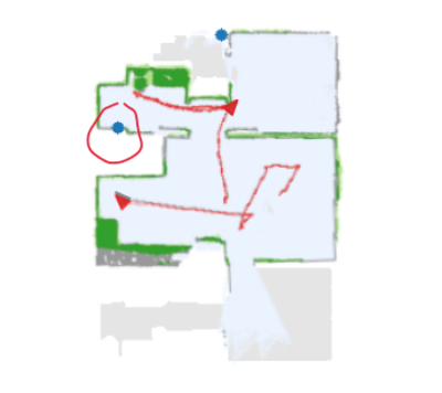
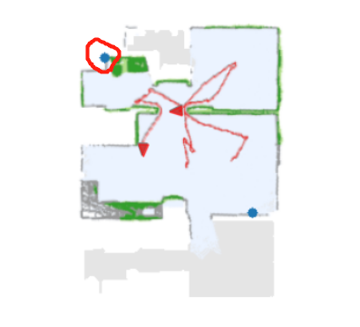
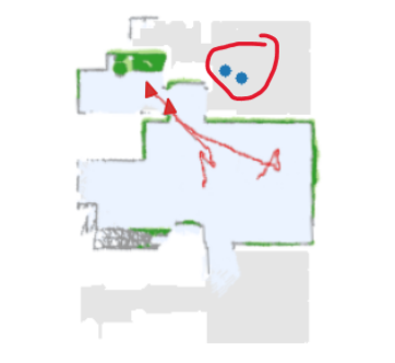
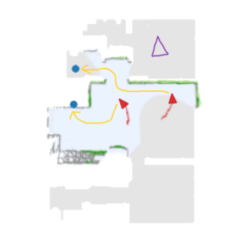
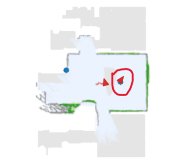
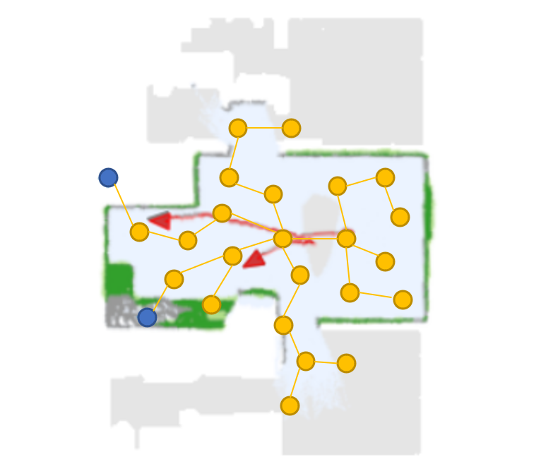
References
- Anguelov et al. (2010) Dragomir Anguelov, Carole Dulong, Daniel Filip, Christian Frueh, Stéphane Lafon, Richard Lyon, Abhijit Ogale, Luc Vincent, and Josh Weaver. Google street view: Capturing the world at street level. Computer, 43(6):32–38, 2010.
- Bhatti et al. (2016) Shehroze Bhatti, Alban Desmaison, Ondrej Miksik, Nantas Nardelli, N Siddharth, and Philip HS Torr. Playing doom with slam-augmented deep reinforcement learning. arXiv preprint arXiv:1612.00380, 2016.
- Bresson et al. (2017) Guillaume Bresson, Zayed Alsayed, Li Yu, and Sébastien Glaser. Simultaneous localization and mapping: A survey of current trends in autonomous driving. IEEE Transactions on Intelligent Vehicles, 2(3):194–220, 2017.
- Burgard et al. (2005) Wolfram Burgard, Mark Moors, Cyrill Stachniss, and Frank E Schneider. Coordinated multi-robot exploration. IEEE Transactions on robotics, 21(3):376–386, 2005.
- Čáp et al. (2013) Michal Čáp, Peter Novák, Jiří Vokřínek, and Michal Pěchouček. Multi-agent rrt*: Sampling-based cooperative pathfinding. arXiv preprint arXiv:1302.2828, 2013.
- Chaplot et al. (2020a) Devendra Singh Chaplot, Dhiraj Gandhi, Saurabh Gupta, Abhinav Gupta, and Ruslan Salakhutdinov. Learning to explore using active neural slam. In International Conference on Learning Representations. ICLR, 2020a.
- Chaplot et al. (2020b) Devendra Singh Chaplot, Dhiraj Prakashchand Gandhi, Abhinav Gupta, and Russ R Salakhutdinov. Object goal navigation using goal-oriented semantic exploration. Advances in Neural Information Processing Systems, 33, 2020b.
- Chaplot et al. (2020c) Devendra Singh Chaplot, Ruslan Salakhutdinov, Abhinav Gupta, and Saurabh Gupta. Neural topological slam for visual navigation. In CVPR, 2020c.
- Chen et al. (2019) Tao Chen, Saurabh Gupta, and Abhinav Gupta. Learning exploration policies for navigation. In International Conference on Learning Representations. ICLR, 2019.
- Chu & Ye (2017) Xiangxiang Chu and Hangjun Ye. Parameter sharing deep deterministic policy gradient for cooperative multi-agent reinforcement learning. CoRR, abs/1710.00336, 2017.
- Cohen (1996) William W Cohen. Adaptive mapping and navigation by teams of simple robots. Robotics and autonomous systems, 18(4):411–434, 1996.
- Desaraju & How (2011) Vishnu R Desaraju and Jonathan P How. Decentralized path planning for multi-agent teams in complex environments using rapidly-exploring random trees. In 2011 IEEE International Conference on Robotics and Automation, pp. 4956–4961. IEEE, 2011.
- Dosovitskiy et al. (2020) Alexey Dosovitskiy, Lucas Beyer, Alexander Kolesnikov, Dirk Weissenborn, Xiaohua Zhai, Thomas Unterthiner, Mostafa Dehghani, Matthias Minderer, Georg Heigold, Sylvain Gelly, et al. An image is worth 16x16 words: Transformers for image recognition at scale. arXiv preprint arXiv:2010.11929, 2020.
- Duan et al. (2017) Yan Duan, Marcin Andrychowicz, Bradly C Stadie, Jonathan Ho, Jonas Schneider, Ilya Sutskever, Pieter Abbeel, and Wojciech Zaremba. One-shot imitation learning. In NIPS, 2017.
- Foerster et al. (2016) Jakob N Foerster, Yannis M Assael, Nando De Freitas, and Shimon Whiteson. Learning to communicate with deep multi-agent reinforcement learning. arXiv preprint arXiv:1605.06676, 2016.
- Fuentes-Pacheco et al. (2015) Jorge Fuentes-Pacheco, José Ruiz-Ascencio, and Juan Manuel Rendón-Mancha. Visual simultaneous localization and mapping: a survey. Artificial intelligence review, 43(1):55–81, 2015.
- Henriques & Vedaldi (2018) Joao F Henriques and Andrea Vedaldi. Mapnet: An allocentric spatial memory for mapping environments. In proceedings of the IEEE Conference on Computer Vision and Pattern Recognition, pp. 8476–8484, 2018.
- Hessel et al. (2019) Matteo Hessel, Hubert Soyer, Lasse Espeholt, Wojciech Czarnecki, Simon Schmitt, and Hado van Hasselt. Multi-task deep reinforcement learning with popart. In Proceedings of the AAAI Conference on Artificial Intelligence, volume 33, pp. 3796–3803, 2019.
- Hu et al. (2020) Junyan Hu, Hanlin Niu, Joaquin Carrasco, Barry Lennox, and Farshad Arvin. Voronoi-based multi-robot autonomous exploration in unknown environments via deep reinforcement learning. IEEE Transactions on Vehicular Technology, 69(12):14413–14423, 2020.
- Iqbal & Sha (2019a) Shariq Iqbal and Fei Sha. Actor-attention-critic for multi-agent reinforcement learning. In International Conference on Machine Learning, pp. 2961–2970. PMLR, 2019a.
- Iqbal & Sha (2019b) Shariq Iqbal and Fei Sha. Coordinated exploration via intrinsic rewards for multi-agent reinforcement learning. arXiv preprint arXiv:1905.12127, 2019b.
- Isler et al. (2016) Stefan Isler, Reza Sabzevari, Jeffrey Delmerico, and Davide Scaramuzza. An information gain formulation for active volumetric 3d reconstruction. In 2016 IEEE International Conference on Robotics and Automation (ICRA), pp. 3477–3484. IEEE, 2016.
- Jain et al. (2019) Unnat Jain, Luca Weihs, Eric Kolve, Mohammad Rastegari, Svetlana Lazebnik, Ali Farhadi, Alexander G Schwing, and Aniruddha Kembhavi. Two body problem: Collaborative visual task completion. In Proceedings of the IEEE/CVF Conference on Computer Vision and Pattern Recognition, pp. 6689–6699, 2019.
- Jiang & Lu (2018) Jiechuan Jiang and Zongqing Lu. Learning attentional communication for multi-agent cooperation. Advances in Neural Information Processing Systems, 31:7254–7264, 2018.
- Jiang et al. (2018) Jiechuan Jiang, Chen Dun, Tiejun Huang, and Zongqing Lu. Graph convolutional reinforcement learning. arXiv preprint arXiv:1810.09202, 2018.
- Juliá et al. (2012) Miguel Juliá, Arturo Gil, and Oscar Reinoso. A comparison of path planning strategies for autonomous exploration and mapping of unknown environments. Autonomous Robots, 33(4):427–444, 2012.
- Kleiner et al. (2006) Alexander Kleiner, Johann Prediger, and Bernhard Nebel. Rfid technology-based exploration and slam for search and rescue. In 2006 IEEE/RSJ International Conference on Intelligent Robots and Systems, pp. 4054–4059. IEEE, 2006.
- Li (2020) Alberto Quattrini Li. Exploration and mapping with groups of robots: Recent trends. Current Robotics Reports, pp. 1–11, 2020.
- Lillicrap et al. (2015) Timothy P Lillicrap, Jonathan J Hunt, Alexander Pritzel, Nicolas Heess, Tom Erez, Yuval Tassa, David Silver, and Daan Wierstra. Continuous control with deep reinforcement learning. arXiv preprint arXiv:1509.02971, 2015.
- Liu et al. (2021a) Iou-Jen Liu, Unnat Jain, Raymond A Yeh, and Alexander Schwing. Cooperative exploration for multi-agent deep reinforcement learning. In International Conference on Machine Learning, pp. 6826–6836. PMLR, 2021a.
- Liu et al. (2021b) Xinzhu Liu, Di Guo, Huaping Liu, and Fuchun Sun. Multi-agent embodied visual semantic navigation with scene prior knowledge. arXiv preprint arXiv:2109.09531, 2021b.
- Long et al. (2020) Qian Long, Zihan Zhou, Abhinav Gupta, Fei Fang, Yi Wu, and Xiaolong Wang. Evolutionary population curriculum for scaling multi-agent reinforcement learning. In International Conference on Learning Representations, 2020.
- Malysheva et al. (2018) Aleksandra Malysheva, Tegg Taekyong Sung, Chae-Bong Sohn, Daniel Kudenko, and Aleksei Shpilman. Deep multi-agent reinforcement learning with relevance graphs. arXiv preprint arXiv:1811.12557, 2018.
- Mnih et al. (2013) Volodymyr Mnih, Koray Kavukcuoglu, David Silver, Alex Graves, Ioannis Antonoglou, Daan Wierstra, and Martin Riedmiller. Playing atari with deep reinforcement learning. arXiv preprint arXiv:1312.5602, 2013.
- Mousavian et al. (2019) Arsalan Mousavian, Alexander Toshev, Marek Fišer, Jana Košecká, Ayzaan Wahid, and James Davidson. Visual representations for semantic target driven navigation. In 2019 International Conference on Robotics and Automation (ICRA), pp. 8846–8852. IEEE, 2019.
- Nazif et al. (2010) Ali Nasri Nazif, Alireza Davoodi, and Philippe Pasquier. Multi-agent area coverage using a single query roadmap: A swarm intelligence approach. In Advances in practical multi-agent systems, pp. 95–112. Springer, 2010.
- Nguyen et al. (2020) Thanh Thi Nguyen, Ngoc Duy Nguyen, and Saeid Nahavandi. Deep reinforcement learning for multiagent systems: A review of challenges, solutions, and applications. IEEE transactions on cybernetics, 50(9):3826–3839, 2020.
- Parisotto & Salakhutdinov (2018) Emilio Parisotto and Ruslan Salakhutdinov. Neural map: Structured memory for deep reinforcement learning. In International Conference on Learning Representations. ICLR, 2018.
- (39) Shivang Patel, Senthil Hariharan, Pranav Dhulipala, Ming C Lin, Dinesh Manocha, Huan Xu, and Michael Otte. Multi-agent ergodic coverage in urban environments.
- Peng et al. (2017) Peng Peng, Quan Yuan, Ying Wen, Yaodong Yang, Zhenkun Tang, Haitao Long, and Jun Wang. Multiagent bidirectionally-coordinated nets for learning to play starcraft combat games. CoRR, abs/1703.10069, 2017. URL http://arxiv.org/abs/1703.10069.
- Ramakrishnan et al. (2020) Santhosh K Ramakrishnan, Ziad Al-Halah, and Kristen Grauman. Occupancy anticipation for efficient exploration and navigation. In European Conference on Computer Vision, pp. 400–418. Springer, 2020.
- Ramakrishnan et al. (2021) Santhosh K Ramakrishnan, Dinesh Jayaraman, and Kristen Grauman. An exploration of embodied visual exploration. International Journal of Computer Vision, 129(5):1616–1649, 2021.
- Rashid et al. (2018) Tabish Rashid, Mikayel Samvelyan, Christian Schroeder, Gregory Farquhar, Jakob Foerster, and Shimon Whiteson. Qmix: Monotonic value function factorisation for deep multi-agent reinforcement learning. In International Conference on Machine Learning, pp. 4295–4304. PMLR, 2018.
- Ryu et al. (2020) Heechang Ryu, Hayong Shin, and Jinkyoo Park. Multi-agent actor-critic with hierarchical graph attention network. In Proceedings of the AAAI Conference on Artificial Intelligence, volume 34, pp. 7236–7243, 2020.
- Savinov et al. (2019) Nikolay Savinov, Anton Raichuk, Raphaël Marinier, Damien Vincent, Marc Pollefeys, Timothy Lillicrap, and Sylvain Gelly. Episodic curiosity through reachability. In International Conference on Learning Representations. ICLR, 2019.
- Savva et al. (2019) Manolis Savva, Abhishek Kadian, Oleksandr Maksymets, Yili Zhao, Erik Wijmans, Bhavana Jain, Julian Straub, Jia Liu, Vladlen Koltun, Jitendra Malik, et al. Habitat: A platform for embodied ai research. In Proceedings of the IEEE/CVF International Conference on Computer Vision, pp. 9339–9347, 2019.
- Schulman et al. (2017) John Schulman, Filip Wolski, Prafulla Dhariwal, Alec Radford, and Oleg Klimov. Proximal policy optimization algorithms. arXiv preprint arXiv:1707.06347, 2017.
- Sethian (1996) James A Sethian. A fast marching level set method for monotonically advancing fronts. Proceedings of the National Academy of Sciences, 93(4):1591–1595, 1996.
- Sukhbaatar et al. (2016) Sainbayar Sukhbaatar, Rob Fergus, et al. Learning multiagent communication with backpropagation. Advances in neural information processing systems, 29:2244–2252, 2016.
- Sunehag et al. (2018) Peter Sunehag, Guy Lever, Audrunas Gruslys, Wojciech Marian Czarnecki, Vinicius Zambaldi, Max Jaderberg, Marc Lanctot, Nicolas Sonnerat, Joel Z Leibo, Karl Tuyls, et al. Value-decomposition networks for cooperative multi-agent learning based on team reward. In Proceedings of the 17th International Conference on Autonomous Agents and MultiAgent Systems, pp. 2085–2087, 2018.
- Tagliabue et al. (2020) Andrea Tagliabue, Stephanie Schneider, Marco Pavone, and Ali-akbar Agha-mohammadi. Shapeshifter: A multi-agent, multi-modal robotic platform for exploration of titan. CoRR, abs/2002.00515, 2020.
- Teh et al. (2017) Yee Whye Teh, Victor Bapst, Wojciech M Czarnecki, John Quan, James Kirkpatrick, Raia Hadsell, Nicolas Heess, and Razvan Pascanu. Distral: Robust multitask reinforcement learning. In NIPS, 2017.
- Terry et al. (2020) Justin K. Terry, Nathaniel Grammel, Ananth Hari, Luis Santos, Benjamin Black, and Dinesh Manocha. Parameter sharing is surprisingly useful for multi-agent deep reinforcement learning. CoRR, abs/2005.13625, 2020.
- Umari & Mukhopadhyay (2017) Hassan Umari and Shayok Mukhopadhyay. Autonomous robotic exploration based on multiple rapidly-exploring randomized trees. In 2017 IEEE/RSJ International Conference on Intelligent Robots and Systems (IROS), pp. 1396–1402, 2017. doi: 10.1109/IROS.2017.8202319.
- Vaswani et al. (2017) Ashish Vaswani, Noam Shazeer, Niki Parmar, Jakob Uszkoreit, Llion Jones, Aidan N Gomez, Ł ukasz Kaiser, and Illia Polosukhin. Attention is all you need. In I. Guyon, U. V. Luxburg, S. Bengio, H. Wallach, R. Fergus, S. Vishwanathan, and R. Garnett (eds.), Advances in Neural Information Processing Systems, volume 30. Curran Associates, Inc., 2017.
- Wakilpoor et al. (2020) Ceyer Wakilpoor, Patrick J Martin, Carrie Rebhuhn, and Amanda Vu. Heterogeneous multi-agent reinforcement learning for unknown environment mapping. arXiv preprint arXiv:2010.02663, 2020.
- Wang et al. (2021) Haiyang Wang, Wenguan Wang, Xizhou Zhu, Jifeng Dai, and Liwei Wang. Collaborative visual navigation. arXiv preprint arXiv:2107.01151, 2021.
- Wang* et al. (2020) Tonghan Wang*, Jianhao Wang*, Yi Wu, and Chongjie Zhang. Influence-based multi-agent exploration. In International Conference on Learning Representations, 2020.
- Wang et al. (2020) Weixun Wang, Tianpei Yang, Yong Liu, Jianye Hao, Xiaotian Hao, Yujing Hu, Yingfeng Chen, Changjie Fan, and Yang Gao. From few to more: Large-scale dynamic multiagent curriculum learning. In Proceedings of the AAAI Conference on Artificial Intelligence, volume 34, pp. 7293–7300, 2020.
- Wang et al. (2018) Xiaolong Wang, Ross Girshick, Abhinav Gupta, and Kaiming He. Non-local neural networks. In Proceedings of the IEEE conference on computer vision and pattern recognition, pp. 7794–7803, 2018.
- Wurm et al. (2008) Kai M Wurm, Cyrill Stachniss, and Wolfram Burgard. Coordinated multi-robot exploration using a segmentation of the environment. In 2008 IEEE/RSJ International Conference on Intelligent Robots and Systems, pp. 1160–1165. IEEE, 2008.
- Xia et al. (2018a) Fei Xia, Amir R. Zamir, Zhiyang He, Alexander Sax, Jitendra Malik, and Silvio Savarese. Gibson Env: real-world perception for embodied agents. In Computer Vision and Pattern Recognition (CVPR), 2018 IEEE Conference on. IEEE, 2018a.
- Xia et al. (2018b) Fei Xia, Amir R Zamir, Zhiyang He, Alexander Sax, Jitendra Malik, and Silvio Savarese. Gibson env: Real-world perception for embodied agents. In Proceedings of the IEEE Conference on Computer Vision and Pattern Recognition, pp. 9068–9079, 2018b.
- Yamauchi (1997a) Brian Yamauchi. A frontier-based approach for autonomous exploration. In Proceedings 1997 IEEE International Symposium on Computational Intelligence in Robotics and Automation CIRA’97.’Towards New Computational Principles for Robotics and Automation’, pp. 146–151. IEEE, 1997a.
- Yamauchi (1997b) Brian Yamauchi. A frontier-based approach for autonomous exploration. In Proceedings 1997 IEEE International Symposium on Computational Intelligence in Robotics and Automation CIRA’97.’Towards New Computational Principles for Robotics and Automation’, pp. 146–151. IEEE, 1997b.
- Yang et al. (2018) Wei Yang, Xiaolong Wang, Ali Farhadi, Abhinav Gupta, and Roozbeh Mottaghi. Visual semantic navigation using scene priors. arXiv preprint arXiv:1810.06543, 2018.
- Yu et al. (2021a) Chao Yu, Akash Velu, Eugene Vinitsky, Yu Wang, Alexandre Bayen, and Yi Wu. The surprising effectiveness of mappo in cooperative, multi-agent games. arXiv preprint arXiv:2103.01955, 2021a.
- Yu et al. (2021b) Jincheng Yu, Jianming Tong, Yuanfan Xu, Zhilin Xu, Haolin Dong, Tianxiang Yang, and Yu Wang. Smmr-explore: Submap-based multi-robot exploration system with multi-robot multi-target potential field exploration method. In 2021 IEEE International Conference on Robotics and Automation (ICRA), 2021b.
- Zambaldi et al. (2018) Vinicius Zambaldi, David Raposo, Adam Santoro, Victor Bapst, Yujia Li, Igor Babuschkin, Karl Tuyls, David Reichert, Timothy Lillicrap, Edward Lockhart, et al. Relational deep reinforcement learning. arXiv preprint arXiv:1806.01830, 2018.
- Zhang et al. (2019a) Chuxu Zhang, Dongjin Song, Chao Huang, Ananthram Swami, and Nitesh V Chawla. Heterogeneous graph neural network. In Proceedings of the 25th ACM SIGKDD International Conference on Knowledge Discovery & Data Mining, pp. 793–803, 2019a.
- Zhang et al. (2019b) Yan Zhang, Jonathon Hare, and Adam Prugel-Bennett. Deep set prediction networks. Advances in Neural Information Processing Systems, 32:3212–3222, 2019b.
- Zhu et al. (2021) Fengda Zhu, Siyi Hu, Yi Zhang, Haodong Hong, Yi Zhu, Xiaojun Chang, and Xiaodan Liang. Main: A multi-agent indoor navigation benchmark for cooperative learning. 2021.