Learning from Failure:
Training Debiased Classifier from Biased Classifier

Junhyun Nam¹ Hyuntak Cha² Sungsoo Ahn¹ Jaeho Lee¹ Jinwoo Shin^1,2
¹School of Electrical Engineering, KAIST
²Graduate School of AI, KAIST
{junhyun.nam, hyuntak.cha, sungsoo.ahn, jaeho-lee, jinwoos}@kaist.ac.kr

Abstract

Neural networks often learn to make predictions that overly rely on spurious correlation existing in the dataset, which causes the model to be biased. While previous work tackles this issue by using explicit labeling on the spuriously correlated attributes or presuming a particular bias type, we instead utilize a cheaper, yet generic form of human knowledge, which can be widely applicable to various types of bias. We first observe that neural networks learn to rely on the spurious correlation only when it is “easier” to learn than the desired knowledge, and such reliance is most prominent during the early phase of training. Based on the observations, we propose a failure-based debiasing scheme by training a pair of neural networks simultaneously. Our main idea is twofold; (a) we intentionally train the first network to be biased by repeatedly amplifying its “prejudice”, and (b) we debias the training of the second network by focusing on samples that go against the prejudice of the biased network in (a). Extensive experiments demonstrate that our method significantly improves the training of network against various types of biases in both synthetic and real-world datasets. Surprisingly, our framework even occasionally outperforms the debiasing methods requiring explicit supervision of the spuriously correlated attributes.

1 Introduction

When trained on carefully curated datasets, deep neural networks achieve state-of-the-art performances on many tasks in artificial intelligence, including image classification [11], object detection [8], and speech recognition [9]. On the other hand, neural networks often dramatically fail when trained on a highly biased dataset, by learning the unintended decision rule that works well only on the dataset being trained on. For instance, it is widely known that object classification datasets suffer from such misleading correlations [23, 29]. As an example, suppose that the “boat” is the only object category appearing in the images with the “water” background. When trained on a dataset with such bias, neural networks often learn to make predictions using the unintended decision rule based on the background of images, whereas a learner intended to learn the decision rule based on the object in the images.

To train a debiased model that captures the “intended correlation” from such biased datasets, recent approaches focus on how to utilize various types of human supervision effectively. One of the most popular forms of such supervision is an explicit label that indicates the misleadingly correlated attribute [14, 18, 24]. For instance, Kim et al. [14], Li and Vasconcelos [18] consider training a model to classify digits (instead of misleadingly correlated color) from the Colored MNIST dataset, under the setup where RGB values for coloring digits are given as side information. Another line of research focuses on developing algorithms tailored to a domain-specific type of bias in the target dataset, whose existence and characteristics are diagnosed by human experts [7, 25, 4, 2]. For instance, Geirhos et al. [7] diagnose that ImageNet-trained classifiers are biased toward texture instead of a presumably more human-aligned notion of shapes, and use this takeaway to construct an augmented dataset to train shape-oriented classifiers.

Acquiring human supervision on the bias, however, is often a dauntingly laborious and expensive task. Gathering explicit labels of such misleadingly correlated attributes requires manual labeling by the workers that have a clear understanding of the underlying bias. Collecting expert knowledge of a human-perceived bias (e.g., texture bias) takes even more effort, as it requires a careful ablation study on the classifiers trained on biased datasets, e.g., Geirhos et al. [7] synthesize data via style transfer [6] to discover the existence of texture bias. Hence, an approach to train a debiased classifier without relying on such expensive supervision is warranted.

Contribution. In this paper, we propose a failure-based debiasing scheme, coined Learning from Failure (LfF). Our scheme does not require expensive supervision on the bias, such as explicit labels of misleadingly correlated attributes, or bias-tailored training technique. Instead, our method utilizes a cheaper form of human knowledge, leveraging the following intriguing observations on neural networks that are being trained on biased datasets.

We first observe that a biased dataset does not necessarily lead the model to learn the unintended decision rule; the bias negatively affects the model only when the bias attribute is “easier” to learn than the target attribute (Section 2.2). For the bias that negatively affects the model, we also observe that samples aligned with the bias show distinct loss trajectories in the training phase compared to samples conflicting with the bias. To be more specific, the classifier learns to fit samples aligned with the bias during the early stage of training and learns samples conflicting with the bias later (Section 2.3). The latter observation lines up with recent findings on training dynamics of deep neural networks [1, 21, 17]; networks tend to defer learning hard concepts, e.g., samples with random labels, to the later phase of training.

Based on the findings, we propose the following debiasing scheme, LfF. We simultaneously train two neural networks, one to be biased and the other to be debiased. Specifically, we train a “biased” neural network by amplifying its early-stage predictions. Here, we employ generalized cross entropy loss [28] for the biased model to focus on easy samples, which are expected to be samples aligned with bias. In parallel, we train a “debiased” neural network by focusing on samples that the biased model struggles to learn, which are expected to be samples conflicting with the bias. To this end, we re-weight training samples using the relative difficulty score based on the loss of the biased model and the debiased model (Section 3).

We show the effectiveness of LfF on various biased datasets, including Colored MNIST [14, 18] with color bias, Corrupted CIFAR-10 [12] with texture bias, and CelebA [19] with gender bias. In addition, we newly construct a real-world dataset, coined biased action recognition (BAR), to resolve the lack of realistic evaluation benchmark for debiasing schemes. In all of the experiments, our method succeeds in training a debiased classifier. In particular, our method improves the accuracy of the unbiased evaluation set by $35.34\%\to 63.39\%$ , $17.93\%\to 31.66\%$ , for the Colored MNIST and Corrupted CIFAR-10¹ datasets, respectively, even when $99.5\%$ of the training samples are bias-aligned (Section 4).

2 A closer look at training deep neural networks on biased datasets

In this section, we describe two empirical observations on training the neural networks with a biased dataset. These observations serve as a key intuition for designing and understanding our debiasing algorithm. We first provide a formal description of biased datasets in Section 2.1. Then we provide our empirical observations in Section 2.2 and Section 2.3.

2.1 Setup

Consider a dataset $\mathcal{D}$ where each input $x$ can be represented by a set of (possibly latent) attributes $\{a_{1},\ldots,a_{k}\}$ for $a_{i}\in\mathcal{A}_{i}$ that describes the input. The goal is to train a predictor $f$ that belongs to a set of intended decision rules $\mathcal{F}_{t}$ , consisting of decision rules that correctly predict the target attribute $y=a_{t}\in\mathcal{A}_{t}$ . We say that a dataset $\mathcal{D}$ is biased, if (a) there exists another attribute $a_{b}\neq y$ that is highly correlated to the target attribute $y$ (i.e., $H(y|a_{b})\approx 0$ ), and (b) one can settle an unintended decision rule $g_{b}\notin\mathcal{F}_{t}$ that correctly classifies $a_{b}$ . We denote such an attribute $a_{b}$ by a bias attribute. In biased datasets with a bias attribute $a_{b}$ , we say that a sample is bias-aligned whenever it can be correctly classified by the unintended decision rule $g_{b}$ , and bias-conflicting whenever it cannot be correctly classified by $g_{b}$ .

Throughout the paper, we consider two types of evaluation datasets: the unbiased and bias-conflicting evaluation sets. We construct the unbiased evaluation set in a way that the target and bias attributes are uncorrelated. To this end, the unbiased evaluation set is constructed to have the same number of samples for every possible value of $(a_{t},a_{b})$ . We simply construct the bias-conflicting evaluation set by excluding bias-aligned samples from the unbiased evaluation set.

Here, we illustrate the examples of biased datasets using the datasets considered for the experiment in Section 2.2 and 2.3, i.e., Colored MNIST and Corrupted CIFAR-10.

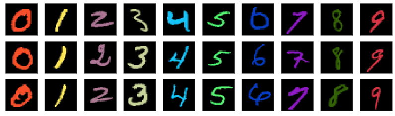
Colored MNIST. We inject color with random perturbation into the MNIST dataset [16] designed for digit classification, resulting in a dataset with two attributes: Digit and Color. In the case of $(a_{t},a_{b})=(\texttt{Digit},\texttt{Color})$ , a set of intended decision rules $\mathcal{F}_{t}$ consists of decision rules that correctly classify images based on the Digit of the images. Here, a decision rule based on other attributes, e.g. Color, is considered as an unintended decision rule. Figure 1(a) illustrates examples of bias-aligned samples, which can be correctly classified by an unintended decision rule based on Color.

2.2 Not all biases are malignant

Table 1: Accuracy of the unbiased evaluation set with varying choice of (target, bias) attribute pair for the Colored MNIST and Corrupted CIFAR-10^1,2 datasets. Accuracy and Accuracy^∗ denotes the performance of the model trained on the biased and unbiased training set, respectively.

Dataset	Target	Bias	Accuracy	Accuracy^∗	Relative drop
Colored MNIST	Color	Digit	99.97 $\pm$ 0.04	100.0 $\pm$ 0.00	0-0.03%
Colored MNIST	Digit	Color	50.34 $\pm$ 0.16	96.41 $\pm$ 0.07	-47.79%
Corrupted CIFAR-10¹	Corruption	Object	98.34 $\pm$ 0.26	99.62 $\pm$ 0.03	0-1.28%
Corrupted CIFAR-10¹	Object	Corruption	22.72 $\pm$ 0.87	80.00 $\pm$ 0.01	-71.60%
Corrupted CIFAR-10²	Corruption	Object	98.64 $\pm$ 0.20	99.80 $\pm$ 0.01	0-1.16%
Corrupted CIFAR-10²	Object	Corruption	21.07 $\pm$ 0.29	79.65 $\pm$ 0.11	-73.56%

Our first observation is that training a classifier with a biased dataset does not necessarily lead to learning an unintended decision rule. Instead, the bias in the dataset negatively affects the prediction only if the bias is easier to be captured by the learned classifier. In Table 1, we report the accuracy of the classifiers for the unbiased evaluation set. We first note the existence of benign bias, i.e., there are cases where the classifier has not been affected by the bias. Particularly, when there is a degradation of accuracy with a certain choice of the target and bias attribute, the degradation does not occur with the choice made in reversed order.

From such an observation, we now define two types of bias: malignant and benign. For a biased dataset $\mathcal{D}$ with a target attribute $y$ and a bias attribute $a_{b}$ , we say this bias is malignant if a model trained on $\mathcal{D}$ suffers performance degradation on unbiased evaluation set compared to one trained on another dataset which is not biased. In contrast, we say bias is benign if a model trained on $\mathcal{D}$ does not suffer such performance degradation. We interpret this observation as follows: the bias attribute inducing malignant bias is “easier” to learn than the target attribute, e.g., Color is easier to learn than Digit. To be specific, the classifier establishes its decision rule by relying on either (a) the intended correlation from the target or (b) the spurious correlation from the bias attribute. If (a) is harder to leverage than (b), the bias becomes malignant since the classifier learns unintended correlation. Otherwise, the classifier learns the correct correlation, hence the bias becomes benign.

2.3 Malignant bias is learned first

Next, we observe that the loss dynamics of bias-aligned samples and bias-conflicting samples during the training phase are in stark contrast, given that the bias is malignant. The loss of bias-aligned samples quickly declines to zero, but the loss of bias-conflicting samples first increases and starts decreasing after the loss of bias-aligned samples reaches near zero.

In Figure 2, we observe a significant difference between training dynamics on the malignant and the benign bias, consistently over the considered datasets. In the case of training under malignant bias, the training loss of the bias-conflicting samples is higher than the loss of the bias-aligned samples, and the gap is more significant during the early stages. In contrast, they are almost indistinguishable when trained under a benign bias.

We make an interesting connection between our observation and the observation made by Arpit et al. [1] on training neural networks on datasets with noisy labels. Arpit et al. [1] analyzed the training dynamics of the neural network on noisy datasets. They empirically demonstrate the preference of neural networks for easy concepts, e.g., common patterns in samples with correct labels, over the hard concepts, e.g., random patterns in samples with incorrect labels. One can interpret our results similarly; since the malignant bias attributes are easier to learn than the original task, the neural network tends to memorize it first.

3 Debiasing by learning from failure (LfF)

Based on our findings in Section 2, we propose a debiasing algorithm, coined Learning from Failure (LfF), for training neural networks on a biased dataset. At a high level, our algorithm simultaneously trains a pair of neural networks $(f_{B},f_{D})$ as follows: (a) intentionally training a model $f_{B}$ to be biased and (b) training a debiased model $f_{D}$ by focusing on the training samples that the biased model struggles to learn. In the rest of this section, we provide details on each component of our debiasing algorithm. We offer a full description of our debiasing scheme in Algorithm 1.

Algorithm 1 Learning from Failure

1: Input:

\theta_{B},\theta_{D}

, training set

\mathcal{D}

, learning rate

\eta

, number of iterations

T

2: Initialize two networks

f_{B}(x;\theta_{B})

and

f_{D}(x;\theta_{D})

3: for

t=1,\cdots,T

4: Draw a mini-batch

\mathcal{B}=\{(x^{(b)},y^{(b)})\}_{b=1}^{B}

from

\mathcal{D}

5: Update

f_{B}(x;\theta_{B})

\theta_{B}\leftarrow\theta_{B}-\eta\nabla_{\theta_{B}}\sum_{(x,y)\in\mathcal{B}}\textrm{GCE}(f_{B}(x),y)

6: Update

f_{D}(x;\theta_{D})

\theta_{D}\leftarrow\theta_{D}-\eta\nabla_{\theta_{D}}\sum_{(x,y)\in\mathcal{B}}\mathcal{W}(x)\cdot\textrm{CE}(f_{D}(x),y)

7: end for

Training a biased model. We first describe how we train the biased model. i.e., the model following the unintended decision rule. From our observation in Section 2, we intentionally strengthen the prediction of the model from the early stage of training to make it follow the unintended decision rule. To this end, we use the following generalized cross entropy (GCE) [28] loss to amplify the bias of the neural network:

\displaystyle\textrm{GCE}(p(x;\theta),y)=\frac{1-p_{y}(x;\theta)^{q}}{q}

where $p(x;\theta)$ and $p_{y}(x;\theta)$ are softmax output of the neural network and its probability assigned to the target attribute of $y$ , respectively. Here, $q\in(0,1]$ is a hyperparameter that controls the degree of amplification. For example, when $\lim_{q\to 0}\frac{1-p^{q}}{q}=-\log p$ , GCE becomes equivalent to standard cross entropy (CE) loss. Compared to the CE loss, the gradient of the GCE loss up-weights the gradient of the CE loss for the samples with a high probability $p_{y}$ of predicting the correct target attribute as follows:

\displaystyle\frac{\partial\textrm{GCE}(p,y)}{\partial\theta}=p_{y}^{q}\frac{\partial\textrm{CE}(p,y)}{\partial\theta},

Therefore, GCE loss trains a model to be biased by emphasizing the “easier” samples with the strong agreement between softmax output of the neural network and the target, which amplifies the “prejudice” of the neural network compare to the network trained with CE.

Training a debiased model. While we train a biased model as described earlier, we also train a debiased model simultaneously with the samples using the CE loss re-weighted by the following relative difficulty score:

\displaystyle\mathcal{W}(x)=\frac{\textrm{CE}(f_{B}(x),y)}{\textrm{CE}(f_{B}(x),y)+\textrm{CE}(f_{D}(x),y)},

where $f_{B}(x),f_{D}(x)$ are softmax outputs of the biased and debiased model, respectively. We use this score to indicate how much each sample is likely to be bias-conflicting to reflect our observation made in Section 2: for bias-aligned samples, biased model $f_{B}$ tends to have smaller loss compare to debiased model $f_{D}$ at the early stage of training, therefore having small weight for training debiased model. In other words, for bias-conflicting samples, biased model $f_{B}$ tends to have larger loss compare to debiased model $f_{D}$ , result in large weight (close to 1) for training debiased model.

4 Experiments

In this section, we demonstrate the effectiveness of our LfF algorithm proposed in Section 3, and introduce our newly constructed biased action recognition dataset, coined BAR. All experimental results in this section support that LfF successfully trains a debiased classifier, with the knowledge that the bias attribute is learned earlier than the target attribute (instead of explicit supervision for the bias present in the dataset). The classifiers trained by LfF consistently outperforms the vanilla classifiers (trained without any debiasing procedure) on both the unbiased and bias-conflicting evaluation set.

For the experiments in this section, we use MLP with three hidden layers, ResNet-20, and ResNet-18 [11] for the Colored MNIST, Corrupted CIFAR-10, and {CelebA, BAR} datasets, respectively. All results reported in this section are averaged over three independent trials. We provide a detailed description of datasets we considered in Appendix A, B and experimental details in Appendix C.

4.1 Controlled experiments

Table 2: Accuracy evaluated on unbiased samples for the Colored MNIST and Corrupted CIFAR-10^1,2 datasets with varying ratio of bias-aligned samples. We denote bias supervision type by (no supervision), (bias-tailored supervision), and (explicit bias supervision). Best performing results are marked in bold.

Dataset	Ratio (%)	Vanilla	Ours	HEX	REPAIR	Group DRO
Dataset	Ratio (%)
Colored MNIST	95.0	77.63 $\pm$ 0.44	85.39 $\pm$ 0.94	70.44 $\pm$ 1.41	82.51 $\pm$ 0.59	84.50 $\pm$ 0.46
	98.0	62.29 $\pm$ 1.47	80.48 $\pm$ 0.45	62.03 $\pm$ 0.24	72.86 $\pm$ 1.47	76.30 $\pm$ 1.53
	99.0	50.34 $\pm$ 0.16	74.01 $\pm$ 2.21	51.99 $\pm$ 1.09	67.28 $\pm$ 1.69	71.33 $\pm$ 1.76
	99.5	35.34 $\pm$ 0.13	63.39 $\pm$ 1.97	41.38 $\pm$ 1.31	56.40 $\pm$ 3.74	59.67 $\pm$ 2.73
Corrupted CIFAR-10¹	95.0	45.24 $\pm$ 0.22	59.95 $\pm$ 0.16	21.74 $\pm$ 0.27	48.74 $\pm$ 0.71	53.15 $\pm$ 0.53
	98.0	30.21 $\pm$ 0.82	49.43 $\pm$ 0.78	17.81 $\pm$ 0.29	37.89 $\pm$ 0.22	40.19 $\pm$ 0.23
	99.0	22.72 $\pm$ 0.87	41.37 $\pm$ 2.34	16.62 $\pm$ 0.80	32.42 $\pm$ 0.35	32.11 $\pm$ 0.83
	99.5	17.93 $\pm$ 0.66	31.66 $\pm$ 1.18	15.39 $\pm$ 0.13	26.26 $\pm$ 1.06	29.26 $\pm$ 0.11
Corrupted CIFAR-10²	95.0	41.27 $\pm$ 0.98	58.57 $\pm$ 1.18	19.25 $\pm$ 0.81	54.05 $\pm$ 1.01	57.92 $\pm$ 0.31
	98.0	28.29 $\pm$ 0.62	48.75 $\pm$ 1.68	15.55 $\pm$ 0.84	44.22 $\pm$ 0.84	46.12 $\pm$ 1.11
	99.0	20.71 $\pm$ 0.29	41.29 $\pm$ 2.08	14.42 $\pm$ 0.51	38.40 $\pm$ 0.26	39.57 $\pm$ 1.04
	99.5	17.37 $\pm$ 0.31	34.11 $\pm$ 2.39	13.63 $\pm$ 0.42	31.03 $\pm$ 0.42	34.25 $\pm$ 0.74

Table 3: Accuracy evaluated on bias-conflicting samples for the Colored MNIST and Corrupted CIFAR-10^1,2 datasets with varying ratio of bias-aligned samples. We denote bias supervision type by (no supervision), (bias-tailored supervision), and (explicit bias supervision). Best performing results are marked in bold.

Dataset	Ratio (%)	Vanilla	Ours	HEX	REPAIR	Group DRO
Dataset	Ratio (%)
Colored MNIST	95.0	75.17 $\pm$ 0.51	85.77 $\pm$ 0.66	67.75 $\pm$ 1.49	83.26 $\pm$ 0.42	83.11 $\pm$ 0.41
	98.0	58.13 $\pm$ 1.63	80.67 $\pm$ 0.56	58.80 $\pm$ 0.28	73.42 $\pm$ 1.42	74.28 $\pm$ 1.93
	99.0	44.83 $\pm$ 0.18	74.19 $\pm$ 1.94	46.96 $\pm$ 1.20	68.26 $\pm$ 1.52	69.58 $\pm$ 1.66
	99.5	28.15 $\pm$ 1.44	63.49 $\pm$ 1.94	35.05 $\pm$ 1.46	57.27 $\pm$ 3.92	57.07 $\pm$ 3.60
Corrupted CIFAR-10¹	95.0	39.42 $\pm$ 0.20	59.62 $\pm$ 0.03	14.09 $\pm$ 0.31	49.99 $\pm$ 0.92	49.00 $\pm$ 0.45
	98.0	22.65 $\pm$ 0.95	48.69 $\pm$ 0.70	9.34 $\pm$ 0.41	38.94 $\pm$ 0.20	35.10 $\pm$ 0.49
	99.0	14.24 $\pm$ 1.03	39.55 $\pm$ 2.56	8.37 $\pm$ 0.56	33.05 $\pm$ 0.36	28.04 $\pm$ 1.18
	99.5	10.50 $\pm$ 0.71	28.61 $\pm$ 1.25	6.38 $\pm$ 0.08	26.52 $\pm$ 0.94	24.40 $\pm$ 0.28
Corrupted CIFAR-10²	95.0	34.97 $\pm$ 1.06	58.64 $\pm$ 1.04	10.79 $\pm$ 0.90	54.46 $\pm$ 1.02	54.60 $\pm$ 0.11
	98.0	20.52 $\pm$ 0.73	48.99 $\pm$ 1.61	6.60 $\pm$ 7.23	44.63 $\pm$ 0.75	42.71 $\pm$ 1.24
	99.0	12.11 $\pm$ 0.29	40.84 $\pm$ 2.06	5.11 $\pm$ 0.59	38.81 $\pm$ 0.20	37.07 $\pm$ 1.02
	99.5	10.01 $\pm$ 0.01	32.03 $\pm$ 2.51	4.22 $\pm$ 0.43	31.45 $\pm$ 0.28	30.92 $\pm$ 0.86

Baselines. For controlled experiments, we compare the performance of our algorithm with other debiasing algorithms, either presuming a particular bias type or requiring access to additional labels containing information about bias attributes. We consider HEX proposed by Wang et al. [25], which attempts to remove texture bias using the bias-specific knowledge. We also consider REPAIR and Group DRO proposed by Li and Vasconcelos [18] and Sagawa et al. [24], requiring explicit labeling of the bias attributes. We provide a detailed description of the employed baselines in Appendix D.

Ratio of the bias-aligned samples. In the first set of experiments, we vary the ratio of bias-aligned samples in the training dataset by selecting from $\{95.0\%,98.0\%,99.0\%,99.5\%\}$ . We experiment on Colored MNIST, and Corrupted CIFAR-10^1,2 datasets with $(a_{t},a_{b})=(\texttt{Digit},\texttt{Color})$ , and $(a_{t},a_{b})=(\texttt{Object},\texttt{Corruption})$ , respectively.

In Table 2, 3, we report the accuracy evaluated on unbiased samples and bias-conflicting samples. We observe that the proposed method significantly outperforms the baseline on all levels of ratio for bias-aligned samples. Most notably, LfF achieves 41.37% accuracy on the unbiased evaluation set for the Corrupted CIFAR-10¹ dataset with 99% bias-aligned samples, while the vanilla model only achieves 22.72%. In addition, we report the accuracy of unbiased evaluation set and bias-conflicting samples with varying levels of difficulty for the bias attributes in Appendix E.

Detailed analysis of failure-based debiasing. We further analyze the specific details of our algorithm. To be precise, we first investigate the accuracies of the vanilla model and the biased, debiased models $f_{B},f_{D}$ trained by our algorithm for the bias-aligned and bias-conflicting samples. In Figure 4, we plot the training curves of each model. We observe both the vanilla model and the biased model easily achieve 100% accuracy for the bias-aligned samples. On the other hand, the vanilla model shows 50% accuracy for the bias-conflicting samples, and the biased model performs close to random guessing. From this result, we can say that our intentionally biased model only exploits the bias attribute without learning the target attribute.

To compare our debiased model to the vanilla model, we start by observing the accuracy gap between the bias-aligned and bias-conflicting samples. As described before, while the vanilla model easily achieves 100% accuracy for the bias-aligned samples, it cannot achieve similar performance for the bias-conflicting samples. In contrast, our debiased model shows consistent performance (about 80%) for both the bias-aligned and bias-conflicting samples. As a result, it indicates that our debiased model successfully learns the intended target attribute, while the predictions of the vanilla model heavily rely on the unintended bias attribute.

Table 4: Accuracy evaluated on the unbiased samples and bias-conflicting samples of the Colored MNIST and Corrupted CIFAR-10^1,2 dataset for ablation of the proposed algorithm. We denote our algorithm using vanilla model as biased model by Ours^†. Best performing results are marked in bold.

Dataset	Unbiased			Bias-conflicting
Dataset	Vanilla	Ours^†	Ours	Vanilla	Ours^†	Ours
Colored MNIST	50.34 $\pm$ 0.16	49.90 $\pm$ 1.67	74.01 $\pm$ 2.21	44.83 $\pm$ 0.18	44.44 $\pm$ 1.83	74.19 $\pm$ 1.94
Corrupted CIFAR-10¹	22.72 $\pm$ 0.87	25.15 $\pm$ 0.63	41.37 $\pm$ 2.34	14.24 $\pm$ 1.03	17.21 $\pm$ 0.69	39.55 $\pm$ 2.56
Corrupted CIFAR-10²	20.71 $\pm$ 0.29	22.90 $\pm$ 0.47	41.29 $\pm$ 2.08	12.11 $\pm$ 0.29	14.89 $\pm$ 0.66	40.84 $\pm$ 2.06

Contribution of GCE loss. We also test a variant of our algorithm, where we train the biased model with standard cross entropy instead of GCE. As observed in Figure 4, the model trained with standard cross entropy, denoted by Vanilla, not only exploits the bias attribute but also partially learns the target attribute. Therefore, one can expect that using such a CE-trained model as the biased model can hurt debiasing ability of our algorithm. In Table 4, we report the test performance of our debiased model trained with the CE-trained biased model instead of the GCE-trained model, denoted as Ours^†. As expected, using the CE-trained model to compute relative difficulty does not help debiasing model.

4.2 Real-world experiments

Table 5: Accuracy evaluated on the unbiased samples and bias-conflicting samples for the CelebA dataset with Gender as the bias attribute.

Target attribute	Unbiased			Bias-conflicting
Target attribute	Vanilla	Ours	Group DRO	Vanilla	Ours	Group DRO
HairColor	70.25 $\pm$ 0.35	84.24 $\pm$ 0.37	85.43 $\pm$ 0.53	52.52 $\pm$ 0.19	81.24 $\pm$ 1.38	83.40 $\pm$ 0.67
HeavyMakeup	62.00 $\pm$ 0.02	66.20 $\pm$ 1.21	64.88 $\pm$ 0.42	33.75 $\pm$ 0.28	45.48 $\pm$ 4.33	50.24 $\pm$ 0.68

CelebA. The CelebA dataset [19] is a multi-attribute dataset for face recognition, equipped with 40 types of attributes for each image. Among 40 attributes, we find that Gender and HairColor attributes have a high correlation. Moreover, we observe the attribute Gender is used as a cue for predicting the attribute HairColor. Therefore, we use HairColor as the target and Gender as the bias attribute. Similarly, we do the same thing for HeavyMakeup as the target and Gender as the bias attribute.

In Table 5, we observe our algorithm consistently outperforms the vanilla model while the vanilla model suffers from gender bias existing in the real-world dataset. The accuracy gap between the vanilla model and our model is larger for the bias-conflicting samples, which indicates the vanilla model fails to learn the intended target attribute, instead exploits the biased statistic of the dataset. Notably, our model is comparable to Group DRO, which requires explicit labeling for the bias attribute (unlike ours), and even outperforms on the unbiased evaluation set when the target attribute is HeavyMakeup. This is because Group DRO aims to maximize the worst-case group accuracy, not overall unbiased accuracy.

Table 6: Class-wise action recognition accuracy on BAR evaluation set. Best performing results are marked in bold.

Action	Climbing	Diving	Fishing	Racing	Throwing	Vaulting	Average
Vanilla	59.05 $\pm$ 17.48	16.56 $\pm$ 1.58	62.69 $\pm$ 3.64	77.27 $\pm$ 2.62	28.62 $\pm$ 2.95	66.92 $\pm$ 7.25	51.85 $\pm$ 5.92
ReBias	77.78 $\pm$ 8.32	51.57 $\pm$ 4.54	54.76 $\pm$ 2.38	80.56 $\pm$ 2.19	28.63 $\pm$ 2.71	65.14 $\pm$ 7.21	59.74 $\pm$ 1.49
Ours	79.36 $\pm$ 4.79	34.59 $\pm$ 2.26	75.39 $\pm$ 3.63	83.08 $\pm$ 1.90	33.72 $\pm$ 0.68	71.75 $\pm$ 3.32	62.98 $\pm$ 2.76

Biased action recognition dataset. To verify effectiveness of our proposed scheme in a realistic setting, we construct a place-biased action recognition (BAR) dataset with training and evaluation set. We settle six typical action-place pairs by inspecting imSitu dataset [27], which provides action and place labels. We assign images describing these six typical action-place pairs to the training set and, otherwise, the evaluation set of BAR. BAR is publicly available¹¹1https://github.com/alinlab/BAR, and a detailed description of BAR is in Appendix B.

BAR aims to resolve the lack of realistic evaluation benchmark for debiasing schemes. Since previous debiasing schemes have tackled certain types of bias, they have assumed the correlation between the target and bias attribute to be tangible, which indeed is not available in the case of real-world settings. Such an assumption also makes it hard to verify whether one’s scheme can be applied to a wide range of realistic settings. BAR instead offers evaluation set which is constructed based on the intuition that “a majority of samples that do not match typical action-place pairs are bias-conflicting.” To demonstrate, the evaluation set consists of samples not matching the settled six typical pairs. In the end, we can use this evaluation set, which would be similar to a set of bias-conflicting samples to verify our algorithm’s effectiveness.

Table 6 illustrates the test accuracy on the BAR evaluation set. LfF outperforms the vanilla classifier for all action classes. This indicates that LfF encourages the model to train on relatively hard training samples, thereby leading to debiasing the model. In addition, LfF outperforms ReBias [2], which is also free from explicit labeling on the bias attribute, for most action classes except Diving.

5 Related work

Debiasing without explicit supervision. In a real-world scenario, bias presented in the dataset often hard to be easily characterized in the form of labels. Even if one can characterize the bias, acquiring explicit supervision for the bias is still an expensive task that requires manual labeling by human labelers, having a clear understanding of the bias. To address this issue, there have been several works to resolve dataset bias, without explicit supervision on the bias. Geirhos et al. [7] observe the presence of texture bias in the ImageNet-trained classifiers, and train shape-oriented classifier with augmented data using style transfer [6]. Wang et al. [25] also aim to remove texture bias, using a hand-crafted module to extract bias and remove captured bias by domain adversarial loss and subspace projection. More recently, Bahng et al. [2] utilize the small-capacity model to capture bias and force debiased model to learn independent feature from the biased model.

Debiasing from the biased model. To train a debiased model, recent works utilize an intentionally biased model to debias another model. These works mainly focused on removing well-known dataset bias that can easily be characterized. Cadene et al. [3] use a question-only model to reduce question bias in a visual question answering (VQA) model. Clark et al. [5] construct bias-only models for the task having prior knowledge of existing biases, including VQA, reading comprehension, and natural language inference (NLI). Concurrently, He et al. [10] also train a biased model that only uses features known to relate to dataset bias in NLI. While these works are limited to biases existing in the NLP domain, Bahng et al. [2] capture local texture bias in image classification and static bias in video action recognition task using small-capacity models.

Previous works mentioned above have leveraged expert knowledge, used as a substitute for explicit supervision, for a particular type of human-perceived bias. We, in a more straightforward approach, consider general properties of bias from observations on training dynamics of bias-aligned and bias-conflicting samples. Although our method also uses a certain form of human knowledge that whether existing bias in the dataset follows our observation, this is a yes/no type of knowledge, which has advantages in its affordability and applicability. We also assume the existence of bias-conflicting samples on which the debiased model should focus, which indeed is the case in real-life application scenarios. In the end, we propose a simple yet widely applicable debiasing scheme free from the choice for form and amount of supervision on the bias.

6 Conclusion

In this work, we propose a debiasing scheme, coined Learning from Failure (LfF), for training neural networks in the biased dataset. Our framework is based on an important observation on relationship between the training of neural networks and the “easiness” of biased attribute. Through extensive experiments, LfF shows successful results on the debiased training of neural networks. We expect our achievements may shed light on the nature of debiasing neural networks with minimal human supervision.

Broader Impact

Mitigating the potential risk caused by biased datasets is a timely subject, especially with the widespread use of AI systems in our daily lives. Since the world is biased by nature, biased models are often deployed without perceiving their discriminative behavior, thereby leading to invoking the potential risk. For instance, a facial recognition software in digital cameras turned out to “over-predict” Asians as blinking when it was trained on Caucasian faces [20]. Disregarding such potential risks would further result in critical social issues [13], such as racism, gender discrimination, filter bubbles [22], and social polarization.

We propose the debiasing scheme to mitigate the aforementioned potential risks. A common approach to reducing the risks is to develop schemes that specifically tackle a bias of interest, e.g., gender, race, etc. However, underexplored biases might exist in the dataset, but bias-specific schemes would not be able to address these other biases. We thus recommend leveraging the general behaviors of neural networks trained on biased datasets, which can be applied for debiasing in diverse applications.

Now we discuss potential benefits and limitations of the proposed scheme. The underexplored types of bias can be discovered by using a set of samples that are hard for the model to learn. Using this approach can increase awareness of underexplored biases. This awareness can be specifically important for groups that would be potentially affected. We acknowledge that assessing the reduction of potential risks by the proposed scheme can be a challenge without specifically identifying the biases. Still, we anticipate that our approach opens a potential to analyze and interpret underexplored types of bias.

Acknowledgements

This work was supported by Institute of Information & communications Technology Planning & Evaluation (IITP) grant funded by the Korea government(MSIT) (No.2019-0-00075, Artificial Intelligence Graduate School Program (KAIST) and No.2019-0-01396, Development of framework for analyzing, detecting, mitigating of bias in AI model and training data)

References

Arpit et al. [2017] D. Arpit, S. Jastrzȩbski, N. Ballas, D. Krueger, E. Bengio, M. S. Kanwal, T. Maharaj, A. Fischer, A. Courville, Y. Bengio, et al. A closer look at memorization in deep networks. In International Conference on Machine Learning, 2017.
Bahng et al. [2020] H. Bahng, S. Chun, S. Yun, J. Choo, and S. J. Oh. Learning de-biased representations with biased representations. In International Conference on Machine Learning, 2020.
Cadene et al. [2019] R. Cadene, C. Dancette, M. Cord, D. Parikh, et al. Rubi: Reducing unimodal biases for visual question answering. In Advances in Neural Information Processing Systems, 2019.
Choi et al. [2019] J. Choi, C. Gao, J. C. Messou, and J.-B. Huang. Why can’t i dance in the mall? learning to mitigate scene bias in action recognition. In Advances in Neural Information Processing Systems, 2019.
Clark et al. [2019] C. Clark, M. Yatskar, and L. Zettlemoyer. Don’t take the easy way out: Ensemble based methods for avoiding known dataset biases. In Conference on Empirical Methods in Natural Language Processing and the International Joint Conference on Natural Language Processing, 2019.
Gatys et al. [2016] L. A. Gatys, A. S. Ecker, and M. Bethge. Image style transfer using convolutional neural networks. In IEEE Conference on Computer Vision and Pattern Recognition, 2016.
Geirhos et al. [2019] R. Geirhos, P. Rubisch, C. Michaelis, M. Bethge, F. A. Wichmann, and W. Brendel. Imagenet-trained CNNs are biased towards texture; increasing shape bias improves accuracy and robustness. In International Conference on Learning Representations, 2019.
Girshick [2015] R. Girshick. Fast r-cnn. In IEEE International Conference on Computer Vision, 2015.
Hannun et al. [2014] A. Hannun, C. Case, J. Casper, B. Catanzaro, G. Diamos, E. Elsen, R. Prenger, S. Satheesh, S. Sengupta, A. Coates, et al. Deep speech: Scaling up end-to-end speech recognition. arXiv preprint arXiv:1412.5567, 2014.
He et al. [2019] H. He, S. Zha, and H. Wang. Unlearn dataset bias in natural language inference by fitting the residual. In Conference on Empirical Methods in Natural Language Processing and the International Joint Conference on Natural Language Processing, 2019.
He et al. [2016] K. He, X. Zhang, S. Ren, and J. Sun. Deep residual learning for image recognition. In IEEE Conference on Computer Vision and Pattern Recognition, 2016.
Hendrycks and Dietterich [2019] D. Hendrycks and T. Dietterich. Benchmarking neural network robustness to common corruptions and perturbations. In International Conference on Learning Representations, 2019.
Holstein et al. [2018] K. Holstein, J. W. Vaughan, H. D. III, M. Dudík, and H. M. Wallach. Improving fairness in machine learning systems: What do industry practitioners need? arXiv preprint arXiv:1812.05239, 2018.
Kim et al. [2019] B. Kim, H. Kim, K. Kim, S. Kim, and J. Kim. Learning not to learn: Training deep neural networks with biased data. In IEEE Conference on Computer Vision and Pattern Recognition, 2019.
Krizhevsky et al. [2009] A. Krizhevsky, G. Hinton, et al. Learning multiple layers of features from tiny images. 2009.
LeCun et al. [1998] Y. LeCun, L. Bottou, Y. Bengio, and P. Haffner. Gradient-based learning applied to document recognition. IEEE, 86(11):2278–2324, 1998.
Lee et al. [2019] K. Lee, S. Yun, K. Lee, H. Lee, B. Li, and J. Shin. Robust inference via generative classifiers for handling noisy labels. In International Conference on Machine Learning, 2019.
Li and Vasconcelos [2019] Y. Li and N. Vasconcelos. Repair: Removing representation bias by dataset resampling. In IEEE Conference on Computer Vision and Pattern Recognition, 2019.
Liu et al. [2015] Z. Liu, P. Luo, X. Wang, and X. Tang. Deep learning face attributes in the wild. In IEEE International Conference on Computer Vision, 2015.
Mehrabi et al. [2019] N. Mehrabi, F. Morstatter, N. Saxena, K. Lerman, and A. Galstyan. A survey on bias and fairness in machine learning. arXiv preprint arXiv:1908.09635, 2019.
Morcos et al. [2018] A. Morcos, M. Raghu, and S. Bengio. Insights on representational similarity in neural networks with canonical correlation. In Advances in Neural Information Processing Systems, 2018.
Pariser [2011] E. Pariser. The Filter Bubble: What the Internet Is Hiding from You. Penguin Group , The, 2011. ISBN 1594203008.
Ribeiro et al. [2016] M. T. Ribeiro, S. Singh, and C. Guestrin. "why should i trust you?" explaining the predictions of any classifier. In ACM SIGKDD International Conference on Knowledge Discovery and Data Mining, 2016.
Sagawa et al. [2020] S. Sagawa, P. W. Koh, T. B. Hashimoto, and P. Liang. Distributionally robust neural networks for group shifts: On the importance of regularization for worst-case generalization. In International Conference on Learning Representations, 2020.
Wang et al. [2019] H. Wang, Z. He, and E. P. Xing. Learning robust representations by projecting superficial statistics out. In International Conference on Learning Representations, 2019.
Yao et al. [2011] B. Yao, X. Jiang, A. Khosla, A. L. Lin, L. J. Guibas, and F.-F. Li. Human action recognition by learning bases of action attributes and parts. In IEEE International Conference on Computer Vision, 2011.
Yatskar et al. [2016] M. Yatskar, L. Zettlemoyer, and A. Farhadi. Situation recognition: Visual semantic role labeling for image understanding. In IEEE Conference on Computer Vision and Pattern Recognition, 2016.
Zhang and Sabuncu [2018] Z. Zhang and M. Sabuncu. Generalized cross entropy loss for training deep neural networks with noisy labels. In Advances in Neural Information Processing Systems, 2018.
Zhu et al. [2017] Z. Zhu, L. Xie, and A. Yuille. Object recognition with and without objects. In International Joint Conference on Artificial Intelligence, 2017.

Appendix A Datasets

A.1 Controlled experiments

We conduct the experiments on biased datasets with the same number of categories for the target and bias attributes, i.e., $|\mathcal{A}_{t}|=|\mathcal{A}_{b}|$ . Furthermore, the empirical distribution $p_{\mathtt{train}}$ of the training dataset is biased to satisfy the following equation:

	$\displaystyle p_{\mathtt{train}}(a_{b}\|a_{t})=\begin{dcases}p_{\mathtt{align}}&\text{if} $g(a_{t})=a_{b}$,\\ \frac{p_{\mathtt{conflict}}}{\|\mathcal{A}_{b}\|-1}&\text{otherwise},\end{dcases}$
	$\displaystyle p_{\mathtt{align}}>p_{\mathtt{conflict}},\quad\sum_{a_{b}\in\mathcal{A}_{b}}p_{\mathtt{train}}(a_{b}\|a_{t})=1.$

Here, $a_{t}$ and $a_{b}$ are the target and bias attribute, respectively. The function $g:\mathcal{A}_{t}\rightarrow\mathcal{A}_{b}$ is a bijection between the target and bias attribute that assigns the bias attribute to each value of the target attribute. $p_{\mathtt{align}}$ , $p_{\mathtt{conflict}}$ are the ratio of bias-aligned and bias-conflicting samples, respectively. In what follows, we describe instance-specific details on the datasets considered in the experiments.

Colored MNIST. The MNIST dataset [16] consists of grayscale digit images. We modify the original MNIST dataset to have two attributes: Digit and Color. Note that similar modification has been proposed by Kim et al. [14], Li and Vasconcelos [18], Bahng et al. [2]. To define the Color attribute, we first choose ten distinct RGB values by drawing them uniformly at random. We use these ten RGB values throughout all the experiments for the Colored MNIST dataset. Then we generate ten Color distributions by assigning chosen RGB values to each Color distribution as its mean. Each Color distribution is a 3-dimensional Gaussian distribution having the assigned RGB value as its mean with predefined covariance $\sigma^{2}I$ . We pair Digit $a_{t}$ and Color distribution $a_{b}$ to make a correlation between two attributes, Digit and Color. Each bias-aligned sample has a Digit colored by RGB value sampled from paired Color distribution, and each bias-conflicting sample has a Digit colored by RGB value sampled from the other (nine) Color distributions. We control the ratio of bias-aligned samples among $\{99.5\%,99.0\%,98.0\%,95.0\%\}$ . The level of difficulty for the bias attribute is defined by the variance ( $\sigma^{2}$ ) of the Color distribution. We vary the standard deviation ( $\sigma$ ) of the Color distributions among $\{0.05,0.02,0.01,0.005\}$ . We use 60,000 training samples and 10,000 test samples.

Corrupted CIFAR-10. This dataset is generated by corrupting the CIFAR-10 dataset [15] designed for object classification, following the protocols proposed by Hendrycks and Dietterich [12]. The resulting dataset consists of two attributes, i.e., category of the Object and type of Corruption used. We use two sets of protocols for Corruption to build two datasets, namely the Corrupted CIFAR-10¹ and the Corrupted CIFAR-10² datasets. In particular, the Corrupted CIFAR-10^1,2 datasets use the following types of Corruption, respectively: {Snow, Frost, Fog, Brightness, Contrast, Spatter, Elastic, JPEG, Pixelate, Saturate} and {GaussianNoise, ShotNoise, ImpulseNoise, SpeckleNoise, GaussianBlur, DefocusBlur, GlassBlur, MotionBlur, ZoomBlur, Original}, respectively. In order to introduce the varying levels of difficulty, we control the “severity” of Corruption, which was predefined by Hendrycks and Dietterich [12]. As the Corruption gets more severe, the images are likely to lose their characteristics and become less distinguishable. We use 50,000 training samples and 10,000 test samples for this dataset.

A.2 Real-world experiments

CelebA. The CelebA dataset [19] is a multi-attribute dataset for face recognition, equipped with 40 types of attributes for each image. Among 40 attributes, we use the BlondHair attribute (denoted by HairColor in the main text) following Sagawa et al. [24], and additionally consider HeavyMakeup attribute as the target attributes. For both of the cases, we use Male attribute (denoted by Gender in the main text) as the bias attribute. The dataset consists of 202,599 face images, and we use the official train-val split for training and test (162,770 for training, 19,867 for test). To evaluate the unbiased accuracy with an imbalanced evaluation set, we evaluate accuracy for each value of $(a_{t},a_{b})$ , and compute average accuracy over all $(a_{t},a_{b})$ pairs.

Appendix B Biased action recognition dataset

6-class action recognition dataset. Biased Action Recognition (BAR) dataset is a real-world image dataset categorized as six action classes which are biased to distinct places. We carefully settle these six action classes by inspecting imSitu [27], which provides still action images from Google Image Search with action and place labels. In detail, we choose action classes where images for each of these candidate actions share common place characteristics. At the same time, the place characteristics of action class candidates should be distinct in order to classify the action only from place attributes. In the end, we settle the six typical action-place pairs as (Climbing, RockWall), (Diving, Underwater), (Fishing, WaterSurface), (Racing, APavedTrack), (Throwing, PlayingField), and (Vaulting, Sky).

The source of dataset. We construct BAR with images from various sources: imSitu [27], Stanford 40 Actions [26], and Google Image Search. In the case of imSitu [27], we merge several action classes where the images have a similar gesture for constructing a single action class of BAR dataset, e.g., {hurling, pitching, flinging} for constructing throwing, and {carting, skidding} for constructing racing.

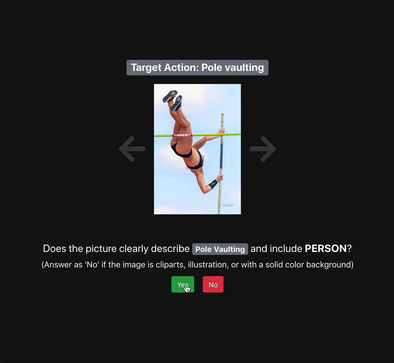
Construction process. BAR consists of training and evaluation sets; images describing the typical six action-place pairs belong to the training set and otherwise, the evaluation set. Before splitting images into these two sets, we exclude inappropriate images: illustrations, clip-arts, images with solid color background, and different gestures with the target gesture of the settled six action-place pairs. Since our sanitized images do not have explicit place labels, we split images into two sets by workers on Amazon Mechanical Turk. We designed the reasoning process to help workers answer the given questions. To be more specific, workers were asked to answer three binary questions. We split images into ‘invalid’, ‘training’, and ‘evaluation’ set based on workers’ responses through binary questions. Workers were also asked to draw a bounding box where they considered it a clue to determine the place in order to help workers filter out images without an explicit clue. Here is the list of binary questions for each action class:

Figure 6: Illustration of BAR reasoning process.

•

Climbing: Does the picture clearly describe Climbing and include person?, Then, is the person rock climbing?, Draw a box around the natural rock wall (including a person) on the image. If it is not natural rock wall, click ‘Cannot find clue‘.
•

Diving: Does the picture clearly describe Scuba Diving / Diving jump / Diving and include person?, Then, does the picture include a body of water or the surface of a body of water?, Draw a box around a body of water or the surface of a body of water (including a person) on the image.
•

Fishing: Does the picture clearly describe Fishing and include person?, Then, does the picture contain the surface of a body of a water?, Draw a box around the surface of a body of a water (including a person) on the image. If the water region does not more than 90% of the image’s background, click ‘Cannot find clue‘.
•

Racing: Does the picture clearly describe Auto racing / Motorcycle racing / Cart racing ?, Then, is the racing held on a paved track?, Draw a box around a paved track (including a vehicle) on the image.
•

Throwing: Does the picture clearly capture the Throwing / Pelting moment and include person?, Then, can you see a type of playing field (baseball mound, football pitch, etc.) where the person is throwing something on?, Draw a box around the playing field (baseball mound, football pitch, etc.) on the image.
•

Vaulting: Does the picture clearly capture the Pole Vaulting and include person?, Then, does the picture contain the sky as background? Draw a box around the sky region (including a person) on the image. If the sky region does not more than 90% of the image’s background, click ‘Cannot find clue‘.

Finally, we use 2,595 images to construct BAR dataset. All image sizes are over 400px width and 300px height. The BAR training and evaluation sets are publicly available on https://anonymous.4open.science/r/c9025a07-2784-47fb-8ba1-77b06c3509fe/.

Table 7: Per-class count of BAR dataset.

Action	Climbing	Diving	Fishing	Racing	Throwing	Vaulting	Total
Training	326	520	163	336	317	279	1941
Evaluation	105	159	42	132	85	131	654

Appendix C Experimental details

Architecture details. For the Colored MNIST dataset, we use the multi-layered perceptron consisting of three hidden layers where each hidden layer consists of 100 hidden units. For the Corrupted CIFAR-10 dataset, we use the ResNet-20 proposed by He et al. [11]. For CelebA and BAR, we employ the Pytorch torchvision implementation of the ResNet-18 model, starting from pretrained weights.

Training details. We use Adam optimizer throughout all the experiments in the paper. We use a learning rate of $0.001$ and a batch size of $256$ for the Colored MNIST and Corrupted CIFAR-10 datasets. We use a learning rate of $0.0001$ and a batch size of $256$ for the CelebA and BAR dataset. Samples were augmented with random crop and horizontal flip transformations for the Corrupted CIFAR-10 and BAR dataset, and horizontal flip transformation for CelebA. For the Corrupted CIFAR-10 dataset, we take $32\times 32$ random crops from image padded by 4 pixels on each side. For the BAR dataset, we take $224\times 224$ random crops using torchvision.transforms.RandomResizedCrop in Pytorch. We do not use data augmentation schemes for training the neural network on the Colored MNIST dataset. We train the networks for 100, 200, 50, and 90 epochs for Colored MNIST, Corrupted CIFAR-10, CelebA and BAR, respectively. The GCE hyperparamter $q=0.7$ is simply taken from the original paper [28]. For stable training of LfF, we use an exponential moving average of loss for computing relative difficulty score instead of loss at each training epoch, with a fixed exponential decay hyperparameter $0.7$ .

Appendix D Baselines

(1) HEX [25] attempts to mitigate texture bias when the texture related domain identifier is not available. By utilizing gray-level co-occurrence matrix (GLCM), neural gray-level co-occurrence Matrix (NGLCM) can capture superficial statistics on the images, and HEX projects the model’s representation orthogonal to the captured texture bias. Since our interest in debiasing is similar to that of HEX in terms of a method without explicit supervision on the bias, we use HEX as a baseline to compare debiasing performance in the case of controlled experiments.

(2) REPAIR [18] “re-weights” training samples to have minimal mutual information between the bias-relevant labels and the intermediate representations of the target classifier. We test all four variants of REPAIR: REPAIR-T, REPAIR-R, REPAIR-C, and REPAIR-S, corresponding to the re-weighting schemes based on thresholding, ranking, per-class ranking, and sampling, respectively. We report the best result among four variants of REPAIR. We use RGB values for coloring digits and classes of corruption as representations inducing bias for the Colored MNIST and Corrupted CIFAR-10 datasets, respectively.

(3) Group DRO [24] aims to minimize “worst-case” training loss over a set of pre-defined groups. Note that one requires additional labels of the bias attribute to define groups to apply group DRO for our problem of interest. With the label of bias attribute, we define $|\mathcal{A}_{t}|\times|\mathcal{A}_{b}|$ groups, one for each value of $(a_{t},a_{b})$ . Sagawa et al. [24] expect that models that learn the spurious correlation between $a_{t}$ and $a_{b}$ in the training data would do poorly on groups for which the correlation does not hold, and hence do worse on the worst-group.

Appendix E Additional experiments

Table 8: Accuracy evaluated on the unbiased samples for the Colored MNIST and Corrupted CIFAR-10^1,2 datasets with varying difficulty of the bias attributes. We denote bias supervision type by (no supervision), (bias-tailored supervision), and (explicit bias supervision). Best performing results are marked in bold.

Dataset	Difficulty	Vanilla	Ours	HEX	REPAIR	Group DRO
Dataset	Difficulty
Colored MNIST	1	50.97 $\pm$ 0.59	75.91 $\pm$ 1.25	51.38 $\pm$ 0.59	69.60 $\pm$ 0.97	70.34 $\pm$ 1.98
	2	50.92 $\pm$ 1.16	74.05 $\pm$ 2.21	51.38 $\pm$ 0.59	64.14 $\pm$ 0.38	70.80 $\pm$ 1.82
	3	49.66 $\pm$ 0.42	72.50 $\pm$ 1.79	52.88 $\pm$ 1.24	69.20 $\pm$ 2.03	71.03 $\pm$ 2.24
	4	50.34 $\pm$ 0.16	74.01 $\pm$ 2.21	51.99 $\pm$ 1.09	67.28 $\pm$ 1.69	71.33 $\pm$ 1.76
Corrupted CIFAR-10¹	1	35.37 $\pm$ 0.58	52.12 $\pm$ 1.99	23.92 $\pm$ 0.80	37.73 $\pm$ 0.73	49.62 $\pm$ 1.49
	2	29.30 $\pm$ 3.11	47.19 $\pm$ 2.26	21.23 $\pm$ 0.38	36.22 $\pm$ 0.88	44.54 $\pm$ 1.70
	3	26.44 $\pm$ 0.98	44.12 $\pm$ 1.53	18.66 $\pm$ 1.16	34.59 $\pm$ 1.88	38.43 $\pm$ 1.44
	4	22.72 $\pm$ 0.87	41.37 $\pm$ 2.34	16.62 $\pm$ 0.80	32.42 $\pm$ 0.35	32.11 $\pm$ 0.83
Corrupted CIFAR-10²	1	32.00 $\pm$ 0.87	46.89 $\pm$ 3.02	20.12 $\pm$ 0.44	41.00 $\pm$ 0.39	44.85 $\pm$ 0.04
	2	27.62 $\pm$ 1.31	43.56 $\pm$ 2.10	16.82 $\pm$ 0.38	39.57 $\pm$ 0.61	43.21 $\pm$ 1.54
	3	22.14 $\pm$ 0.03	41.46 $\pm$ 0.30	15.22 $\pm$ 0.47	38.16 $\pm$ 0.52	42.12 $\pm$ 0.52
	4	20.71 $\pm$ 0.29	41.29 $\pm$ 2.08	14.42 $\pm$ 0.51	38.40 $\pm$ 0.26	39.57 $\pm$ 1.04

Table 9: Accuracy evaluated on the bias-conflicting samples for the Colored MNIST and Corrupted CIFAR-10^1,2 datasets with varying difficulty of the bias attributes. We denote bias supervision type by (no supervision), (bias-tailored supervision), and (explicit bias supervision). Best performing results are marked in bold.

Dataset	Difficulty	Vanilla	Ours	HEX	REPAIR	Group DRO
Dataset	Difficulty
Colored MNIST	1	51.32 $\pm$ 0.45	68.03 $\pm$ 1.11	50.54 $\pm$ 0.88	67.70 $\pm$ 1.02	68.77 $\pm$ 1.26
	2	45.54 $\pm$ 0.65	75.56 $\pm$ 1.22	46.84 $\pm$ 0.44	63.71 $\pm$ 0.29	69.28 $\pm$ 1.13
	3	45.48 $\pm$ 1.29	74.29 $\pm$ 1.78	47.88 $\pm$ 1.37	70.05 $\pm$ 2.10	68.68 $\pm$ 1.26
	4	44.83 $\pm$ 0.18	74.19 $\pm$ 1.94	46.96 $\pm$ 1.20	68.26 $\pm$ 1.52	69.58 $\pm$ 1.66
Corrupted CIFAR-10¹	1	44.23 $\pm$ 2.61	43.76 $\pm$ 1.16	35.50 $\pm$ 2.82	38.11 $\pm$ 0.68	57.34 $\pm$ 1.33
	2	28.47 $\pm$ 0.63	49.04 $\pm$ 2.08	16.82 $\pm$ 1.01	36.81 $\pm$ 0.93	45.03 $\pm$ 1.66
	3	21.71 $\pm$ 3.37	44.22 $\pm$ 2.69	13.46 $\pm$ 0.41	35.15 $\pm$ 1.88	39.64 $\pm$ 1.91
	4	14.24 $\pm$ 1.03	39.55 $\pm$ 2.56	8.37 $\pm$ 0.56	33.05 $\pm$ 0.36	28.04 $\pm$ 1.18
Corrupted CIFAR-10²	1	30.56 $\pm$ 0.39	46.27 $\pm$ 2.66	22.51 $\pm$ 0.45	41.19 $\pm$ 0.32	43.64 $\pm$ 1.45
	2	24.70 $\pm$ 1.03	44.74 $\pm$ 3.01	19.37 $\pm$ 0.41	39.99 $\pm$ 0.57	40.94 $\pm$ 0.34
	3	19.77 $\pm$ 1.44	41.72 $\pm$ 1.90	16.14 $\pm$ 0.28	38.41 $\pm$ 0.48	40.61 $\pm$ 2.01
	4	12.11 $\pm$ 0.29	40.84 $\pm$ 2.06	5.11 $\pm$ 0.59	38.81 $\pm$ 0.20	37.07 $\pm$ 1.02

Difficulty of the bias attribute. In addition to varying ratio of bias-conflicting samples, we vary the level of “difficulty” for the biased attributes by controlling how much the target attribute is easy to distinguish from the given image. Based on our observations in Section 2, the difficulty of bias is lower, the more likely the classifier is to suffer from bias. We introduce four levels of difficulty for the Colored MNIST and Corrupted CIFAR-10^1,2 datasets with the target and the biased attribute chosen as (Digit, Color) and (Object, Corruption), respectively. For the Colored MNIST dataset, we vary the standard deviation of the Gaussian noise for perturbing the RGB values of injected color. In cases of Corrupted CIFAR-10, we control the “severity” of Corruption, which was predefined by Hendrycks and Dietterich [12]. We provide a detailed description of difficulty of the bias attribute in Appendix A.

In Table 8, 9, we again observe our algorithm to consistently outperform the baseline algorithm by a large margin, regardless of the difficulty for the biased attribute. Furthermore, we observe that both baseline and LfF trained classifiers get more biased as the difficulty of the bias attribute increase in general, which also validates our claims made in Section 2. Notably, LfF even outperforms the baseline methods that utilizes explicit label on the bias attribute in most cases.

Table 10: Accuray evaluated on the unbiased samples and bias-conflicting samples for the Colored MNIST datasets with varying ratio of bias-aligned samples.

Dataset	Ratio (%)	Unbiased			Bias-conflicting
Dataset	Ratio (%)	Vanilla	Ours	RUBi	Vanilla	Ours	RUBi
Colored MNIST	95.0	77.63 $\pm$ 0.44	85.39 $\pm$ 0.94	78.22 $\pm$ 0.34	75.17 $\pm$ 0.51	85.77 $\pm$ 0.66	75.84 $\pm$ 0.36
	98.0	62.29 $\pm$ 1.47	80.48 $\pm$ 0.45	64.92 $\pm$ 0.78	58.13 $\pm$ 1.63	80.67 $\pm$ 0.56	61.04 $\pm$ 0.83
	99.0	50.34 $\pm$ 0.16	74.01 $\pm$ 2.21	52.41 $\pm$ 0.42	44.83 $\pm$ 0.18	74.19 $\pm$ 1.94	46.85 $\pm$ 0.46
	99.5	35.34 $\pm$ 0.13	63.39 $\pm$ 1.97	36.42 $\pm$ 0.37	28.15 $\pm$ 1.44	63.49 $\pm$ 1.94	29.36 $\pm$ 0.43

Comparison to other combination rule. There have been several works that utilize intentionally biased models to debias another model. RUBi proposed by Cadene et al. [3] masks original prediction with the mask obtained from the prediction of the biased model. LearnedMixin proposed by Clark et al. [5] uses an ensemble of logits of two models. DRiFt proposed by He et al. [10] learns residual of the pretrained biased model to obtain the debiased model. As an effort to keep the usage of human knowledge minimal, we designed our combination rule without any hyperparameter. In Table 10, we constructed an ablation study on LfF with a combination rule replaced by that of RUBi. While our method equipped with the RUBi combination rule slightly improves accuracy over the vanilla model, it is far behind other resampling/reweighting based methods like REPAIR and Group DRO. In conclusion, resampling/reweighting based methods are generally effective method than manipulating the predictions or logits directly.

Learning from Failure: Training Debiased Classifier from Biased Classifier