Learning from Label Proportions
with Instance-wise Consistency

Ryoma Kobayashi
The University of Tokyo
kobayashi@mi.t.u-tokyo.ac.jp
&Yusuke Mukuta
The University of Tokyo / RIKEN
mukuta@mi.t.u-tokyo.ac.jp
&Tatsuya Harada
The University of Tokyo / RIKEN
harada@mi.t.u-tokyo.ac.jp

Abstract

Learning from Label Proportions (LLP) is a weakly supervised learning method that aims to perform instance classification from training data consisting of pairs of bags containing multiple instances and the class label proportions within the bags. Previous studies on multiclass LLP can be divided into two categories according to the learning task: per-instance label classification and per-bag label proportion estimation. However, these methods often results in high variance estimates of the risk when applied to complex models, or lack statistical learning theory arguments. To address this issue, we propose new learning methods based on statistical learning theory for both per-instance and per-bag policies. We demonstrate that the proposed methods are respectively risk-consistent and classifier-consistent in an instance-wise manner, and analyze the estimation error bounds. Additionally, we present a heuristic approximation method that utilizes an existing method for regressing label proportions to reduce the computational complexity of the proposed methods. Through benchmark experiments, we demonstrated the effectiveness of the proposed methods. ¹¹1Our code is available at https://github.com/ryoma-k/LLPIWC.

1 Introduction

With the development of machine learning—particularly deep learning—there has been a recent surge of interest in techniques for learning from incomplete observational data. This field, which is known as weakly supervised learning, encompasses various approaches for dealing with incomplete or noisy data, such as semi-supervised learning Chapelle et al. (2006); Zhu and Goldberg (2009); Sakai et al. (2017), label noise learning Natarajan et al. (2013); Han et al. (2018), multiple instance learning Amores (2013); Ilse et al. (2018), partial label learning Feng et al. (2020); Lv et al. (2020), complementary label learning Ishida et al. (2017), positive unlabeled learning du Plessis et al. (2014), positive confidence learning Ishida et al. (2018), similar unlabeled learning Bao et al. (2018), and similar dissimilar learning Shimada et al. (2021). Each of these properties was clarified according to statistical learning theory Sugiyama et al. (2022).

Learning from Label Proportions (LLP)—a weakly supervised learning method that is the focus of this study—involves learning instance classification problems using pairs of bags consisting of instances and their class-label proportions. LLP has been applied in various domains, including image and video analysis Chen et al. (2014); Lai et al. (2014); Ding et al. (2017); Li and Taylor (2015), physics Dery et al. (2017); Musicant et al. (2007), medicine Hernández-González et al. (2018); Bortsova et al. (2018), and activity analysis Poyiadzi et al. (2018).

In this study, we focus on multiclass LLP (MCLLP), which can be divided into two categories according to the learning task: per-instance label classification Zhang et al. (2022); Dulac-Arnold et al. (2019); Liu et al. (2021) and per-bag label proportion estimation Ardehaly and Culotta (2017); Liu et al. (2019); Tsai and Lin (2020); Yang et al. (2021); BaruÄiÄ and Kybic (2022). The existing method for the former Zhang et al. (2022) is based on statistical learning theory and exhibits classification performance consistency. It estimates the overall expected losses and, as we show later, tends to misestimate the risk—particularly when applied to complex models such as deep learning models. For the latter, the existing methods rely on empirical techniques, such as regressing class proportions by averaging instance outputs Ardehaly and Culotta (2017). However, these studies lacked a clear statistical foundation.

To address these issues, we propose two new MCLLP methods: one for per-instance label classification and one for per-bag label proportion classification. The first method employs a risk-consistent approach utilizing a loss function equivalent to supervised learning for each individual instance along with their expectations. In contrast, the second method employs a classifier-consistent approach, producing an instance classifier equivalent to those obtained through supervised learning; the proof is again discussed for each individual instance. In addition, we present a heuristic approximation method to reduce the computational complexity of these methods, which utilizes the average operation commonly employed in existing per-bag learning approaches. The contributions of this study can be summarized as follows.

•

We introduce two MCLLP methods for per-instance label and per-bag label proportion classification and prove their consistency in an instance-wise manner. We also derive bounds for their estimation errors.
•

We analyze the method using the mean output operation Ardehaly and Culotta (2017) and demonstrate that it can be perceived as a maximization of the likelihood of label proportions. Then, we propose a heuristic approximation method using this operation to reduce the computational complexity of our methods.

2 Formulations and Related Studies

In this section, we introduce standard multiclass classification, LLP, and partial label learning (PLL) and subsequently review related studies.

2.1 Standard Multiclass Classification

In $C$ -class classification, let $\mathcal{X}$ be the input space and $\mathcal{Y}=\{1,...,C\}$ be the space of the labels. Typically, we assume that data $(x,y)\in(\mathcal{X},\mathcal{Y})$ are independently sampled from the probability distribution $p(x,y)$ . Let $\ell\colon\mathbb{R}^{k}\times\mathcal{Y}\rightarrow\mathbb{R}_{\geq 0}$ denotes the multiclass loss function, which measures the difference between the label and predicted output. The goal of multiclass classification is to minimize the subsequent predictive loss for the hypothesis $f\colon\mathcal{X}\rightarrow\mathbb{R}^{C}$ .

\displaystyle R(f)=\underset{(x,y)\sim p(x,y)}{\mathbb{E}}[\ell(f(x),y)].

(1)

In practice, $p(x,y)$ is unobserved, and we use training data $\tilde{D}=\{(x_{i},y_{i})\}_{i=1}^{n}$ to minimize the empirical loss Vapnik (1998):

\displaystyle\hat{R}(f)=\frac{1}{n}\sum_{i=1}^{n}\ell(f(x_{i}),y_{i}).

A method is called risk-consistent if it has the same risk as Eq. 1, whereas a method is called classifier-consistent if it yields the same optimal classifier as the supervised classifier.

2.2 LLP

In LLP, pairs of bags consisting of multiple instances and the proportion of labels they contain are given. In this study, we formulate LLP using unordered pairs that allow overlap, that is, multisets, instead of the proportions of class labels. Hereinafter, the multiset is denoted by $\{|\cdot|\}$ , for example, $\{|1,1,2|\}$ . Let $\mathcal{X}^{K}$ and $\mathcal{Y}^{K}$ be the direct product spaces of bags and labels, respectively, with K instances, and let $\mathcal{S}^{K}$ be the space of label multisets. With training data $\tilde{D}=\{(X_{i},S_{i})\in(\mathcal{X}^{K},\mathcal{S}^{K})\}_{i=1}^{n}$ , we represent each instance and label as $X_{i}=(X_{i}^{(1)},...,X_{i}^{(K)})$ and $Y_{i}=(Y_{i}^{(1)},...,Y_{i}^{(K)})$ , where the top and bottom subscripts associate them with a particular bag. Furthermore, we define $\mathcal{Y}_{\sigma(S)}^{K}$ as the set of all possible label assignments from the label multiset $S$ :

\displaystyle\mathcal{Y}_{\sigma(S)}^{K}:=\left\{Y\in\mathcal{Y}^{K}\middle|\{|Y^{(1)},...,Y^{(K)}|\}=S\right\}.

The LLP then assumes that the following holds:

\displaystyle P(S_{i}|X_{i},Y_{i})=P(S_{i}|Y_{i})=\begin{cases}1&\text{if~{}~{}~{}}Y_{i}\in\mathcal{Y}_{\sigma(S_{i})}^{K},\\ 0&\text{otherwise.}\end{cases}

(2)

Various techniques have been applied to address LLP, including linear models Wang and Feng (2013); Cui et al. (2017); Pérez-Ortiz et al. (2016), support vector machines Rüping (2010); Yu et al. (2013); Qi et al. (2017); Cui et al. (2016); Shi et al. (2019); Chen et al. (2017); Wang et al. (2015); Lu et al. (2019a), a clustering algorithm Stolpe and Morik (2011), Bayesian networks Hernández-González et al. (2013, 2018), random forest Shi et al. (2018), and graph-based approaches Poyiadzi et al. (2018). Here, we focus on the learning tasks used in existing research and divide them into two categories: per-instance label classification and per-bag label proportion estimation.

The learning task of per-instance label classification can be further divided into two policies. The initial policy estimates the parameters or losses by utilizing an equation that holds only for expectations. This policy has been the subject of longstanding investigations in the field of LLP and has been analyzed using statistical learning theory Quadrianto et al. (2009); Patrini et al. (2014); Lu et al. (2019b); Scott and Zhang (2020). As an example of a study related to MCLLP, Zhang et al. (2022) recently proposed an extension of the binary classification LLP method using label noise forward correction Scott and Zhang (2020) for MCLLP and achieved classifier-consistency. However, it is important to note that the hypothesis that minimizes the loss of label noise is equivalent to the hypothesis that minimizes the loss of supervised learning on expectation but not necessarily on the loss for each instance. Therefore, using complex models such as deep learning may lead to high variance estimation of the risk, and as discussed in Sec. 6, its classification performance may not be as high as that of the other methods. Tang et al. (2022) proposed a technique utilizing label noise backward correction with the constraint of per-bag loss. Statistical analysis of this constraint has yet to be conducted.

The other policy for taking loss per instance is to take classification loss by creating pseudo-labels. Dulac-Arnold et al. (2019) and Liu et al. (2021) proposed creating pseudo-labels using entropy-constrained optimal transport and taking per-instance losses. However, these methods lack a statistical background, and their properties are unclear.

To estimate per-bag label proportions, Yu et al. (2015) introduced Empirical Proportion Risk Minimization (EPRM), which involves empirical risk minimization for the bag proportions in the binary setting. Under the assumptions of the bag generation process and distribution of the model outputs, they showed that the instance classification error can be bounded by the classification error of the label proportion. Building on this approach, Ardehaly and Culotta (2017) proposed Deep LLP (DLLP) as an extension of EPRM for handling multiple classes. DLLP aims to minimize the Kullback–Leibler divergence between the predicted mean probabilities for each class, which is represented by $\bar{p}(y=c|X_{i}):=\frac{1}{K}\sum_{k}p(y=c|X_{i}^{(k)})$ , and the proportion of each class within a bag, which is represented by $p(y=c|S_{i})=\frac{1}{K}\sum_{y\in S}\mathbbm{1}\{y=c\}$ , as follows:

\displaystyle L_{prop}=-\sum_{c}p(y=c|S_{i})\log(\bar{p}(y=c|X_{i})).

(3)

In subsequent studies, DLLP was applied to self-supervised Tsai and Lin (2020), contrastive learning Yang et al. (2021), and semi-supervised learning using generative adversarial networks Liu et al. (2019), although the use of the mean operation for these methods is not fully understood, and the consistency of instance classification is yet to be demonstrated in multiclass settings. As a method that does not use the mean operation, BaruÄiÄ and Kybic (2022) proposed a method that maximizes the likelihood of bag proportions using the EM algorithm. However, its background based on statistical learning theory has not been shown.

2.3 PLL

PLL involves predicting the correct label when multiple candidate labels are provided. MCLLP can be viewed as a PLL setting by treating all labels given for a particular bag as potential candidates.

A notable contribution to the field of PLL was PRODEN Lv et al. (2020), which progressively updates the labels of instances during the learning process and was shown to be risk-consistent Feng et al. (2020). A more generalized risk Wu et al. (2022) is expressed as follows:

\displaystyle R_{PLLrc}(f)=\underset{p(x,S)}{\mathbb{E}}[\sum_{y\in S}\frac{P(y|x)}{P(S|x)}\ell(f(x),y)].

(4)

Feng et al. (2020) showed that a classifier-consistent method can be realized by classifying label candidates under the assumption of a distribution of partial labels. If the probability that the random variable representing a candidate label is $S=T_{j}$ is estimated using a multivalued function $q_{j}(x)=P(S=T_{j}|x)$ , the risk is expressed as

\displaystyle R_{PLLcc}(f)=\underset{p(x,S)}{\mathbb{E}}[\ell(q(x),S)].

(5)

Inspired by PLL methods based on statistical learning theory, we propose a learning method involving per-instance label classification and per-bag label proportion classification.

3 Per-Instance Method

In this section, we propose a method for MCLLP that involves per-instance label classification. We demonstrate that our method is risk-consistent and present a learning procedure following the computation of its estimation error bounds.

3.1 Risk Estimation

We assume instance label independence, as follows:

\displaystyle P(Y|X)=\Pi_{i=1}^{K}P(Y^{(i)}|X^{(i)}).

(6)

Let $\mathit{set}(S)$ be the set of elements of multiset $S$ excluding duplicates, for example, $\mathit{set}(\{|1,1,2|\})=\{1,2\}$ . The probability of a pair of bags and their labels $P(X,Y)$ can be transformed using the pair $(X,S)$ of a bag and its label proportion as follows:

	$\displaystyle P(X,Y)$	$\displaystyle=\sum_{S\in\mathcal{S}^{K}}P(X,Y,S)=\sum_{S\in\mathcal{S}^{K}}P(X,S)\frac{P(X,Y,S)}{P(X,S)}$
		$\displaystyle=\sum_{S\in\mathcal{S}^{K}}P(X,S)\frac{P(Y,S\|X)}{P(S\|X)}$		(7)

\displaystyle P(Y,S|X)=P(S|X,Y)P(Y|X)\overset{(\ref{eq:PSXY})}{=}\begin{cases}P(Y|X)&\text{if~{}~{}~{}}Y\in\mathcal{Y}_{\sigma(S)}^{K},\\ 0&\text{otherwise}\end{cases}

(8)

	$\displaystyle P(S\|X)$	$\displaystyle=\sum_{Y\in\mathcal{Y}^{K}}P(Y,S\|X)\overset{(\ref{eq:PYSX})}{=}\sum_{Y\in\mathcal{Y}_{\sigma(S)}^{K}}P(Y\|X)$
		$\displaystyle\overset{(\ref{eq:PYX})}{=}\sum_{y\in\mathit{set}(S)}P(y\|X^{(k)})P(S\backslash y\|X\backslash X^{(k)}).$		(9)

The risk function $R(f)$ used in ordinary supervised learning can be transformed using these relationships, yielding the following expression:

		$\displaystyle{}R(f)=\underset{p(x,y)}{\mathbb{E}}\left[\ell(f(x),y)\right]=\frac{1}{K}\underset{p(X,Y)}{\mathbb{E}}\left[\sum_{k}\ell(f(X^{(k)}),Y^{(k)})\right]$
		$\displaystyle=\frac{1}{K}\int_{\mathcal{X}^{K}}\sum_{Y\in\mathcal{Y}^{K}}P(X,Y)\sum_{k}\ell(f(X^{(k)}),Y^{(k)})dX$
		$\displaystyle\overset{(\ref{eq:PXY})}{=}\frac{1}{K}\int_{\mathcal{X}^{K}}\sum_{Y\in\mathcal{Y}^{K}}\sum_{S\in\mathcal{S}^{K}}P(X,S)\frac{P(Y,S\|X)}{P(S\|X)}\sum_{k}\ell(f(X^{(k)}),Y^{(k)})dX$
		$\displaystyle\overset{(\ref{eq:PYSX})}{=}\frac{1}{K}\underset{p(X,S)}{\mathbb{E}}\left[\sum_{Y\in\mathcal{Y}_{\sigma(S)}^{K}}\frac{P(Y\|X)}{P(S\|X)}\sum_{k}\ell(f(X^{(k)}),Y^{(k)})\right]$
		$\displaystyle\overset{(\ref{eq:PSX})}{=}\frac{1}{K}\underset{p(X,S)}{\mathbb{E}}\left[\sum_{k}\sum_{y\in\mathit{set}(S)}\frac{P(y\|X^{(k)})P(S\backslash y\|X\backslash X^{(k)})}{\sum_{y^{\prime}\in\mathit{set}(S)}P(y^{\prime}\|X^{(k)})P(S\backslash y^{\prime}\|X\backslash X^{(k)})}\ell(f(X^{(k)}),y)\right]$
		$\displaystyle:=R_{rc}(f).$		(10)

We define $R_{rc}$ as the risk estimated from a pair $(X,S)$ of instance sets and label proportions in Sec. 3.1. From this equation, it is possible to learn the possible label candidates $y$ from a given label multiset $S$ by weighting the typical supervised learning loss.

3.2 Risk-Consistency & Estimation Error Bound

We begin by confirming that our method is risk-consistent. It is shown from Sec. 3.1 that the proposed risk is the same as that in supervised learning. We emphasize that each instance takes the same loss as supervised learning by Sec. 3.1.

In the following section, we analyze the estimation error bounds for this loss. It is assumed that $P(y|X^{(k)})$ is fixed. Let $\hat{f}_{rc}=\min_{f\in\mathcal{F}}\hat{R}_{rc}(f)$ and $f_{rc}^{*}=\min_{f\in\mathcal{F}}R_{rc}(f)$ be hypotheses to minimize the empirical risk and predictive risk, respectively. Let the hypothesis space be $\mathcal{H}_{y}:\{h:x\rightarrow f_{y}(x)|f\in\mathcal{F}\}$ , and let $\mathfrak{R}_{n}(\mathcal{H}_{y})$ be the expected Rademacher complexity of $\mathcal{H}_{y}$ Bartlett and Mendelson (2002). Suppose that the loss function $\ell(f(x),y)$ is $\rho$ -Lipschitz with respect to the inputs and bounded by $M$ .

Theorem 3.1.

For any $\delta>0$ , we have with probability at least $1-\delta$ ,

\displaystyle R_{rc}(\hat{f}_{rc})

\displaystyle-R_{rc}(f_{rc}^{*})\leq 4\sqrt{2}\rho\sum_{y=1}^{C}\mathfrak{R}_{n}(\mathcal{H}_{y})+2M\sqrt{\frac{\log\frac{2}{\delta}}{2n}}.

The proof is provided in Sec. A.1. In general, $\mathfrak{R}_{n}(\mathcal{H}_{y})$ is bounded by some positive constant $\mathcal{C}_{\mathcal{H}}/\sqrt{n}$ Golowich et al. (2018), which indicates the convergence of $f_{rc}$ to $f_{rc}^{*}$ as $n\rightarrow\infty$ .

3.3 Learning Method

In the actual learning process, given that $P(y|X^{(k)})$ values are unknown during the learning process, it is necessary to estimate them. As a learning method, we progressively update $P(y|X^{(k)})$ simultaneously, similar to PRODEN Lv et al. (2020). This method is presented in Algorithm 1. We define this method as RC method.

Algorithm 1 RC / RC_Approx Algorithm

Input: Model

f

, epoch

T_{max}

, proportions labeled training set

\tilde{D}=\{(X_{i},S_{i})\}_{i=1}^{n}

Initialize

P(y|X_{i}^{(k)})=\frac{1}{K}\sum_{y\in S_{i}}\mathbbm{1}\{y=c\}

for

t=1

T_{max}

Shuffle

\tilde{D}

into

B

mini-batches.

for

b=1

B

COMPUTE

\hat{P}

= softmax(

f(X_{i}^{k})

UPDATE

f

by Sec. 3.1.

UPDATE

P(Y_{i}^{(k)}=y|X_{i}^{(k)})

\hat{P}

end for

4 Per-Bag Method

In this section, we describe a classifier-consist method that involves per-bag label proportion classification and provide a detailed description of the learning procedure, including the calculation of the estimation error bounds.

4.1 Risk Estimation

For a given label multiset variable $S$ , there are ${}_{K}H_{C}=\frac{(K+C-1)!}{K!(C-1)!}$ candidates, and the space of the label multiset $\mathcal{S}^{K}$ can be represented as $\mathcal{S}^{K}=\{T_{j}|j\in\{1,\cdots,{}_{K}H_{C}\}\}$ . We propose classifying the multiset $T_{j}$ and estimating the probability $P(S=T_{j}|X)$ using each instance output $e(y=c|X^{(k)})$ , where $e$ denotes the softmax of the outputs. In accordance with Sec. 3.1, we design a multivalued function $q$ such that the $j$ th output is $q_{j}(X)=P(S=T_{j}|X)$ , as follows:

\displaystyle q_{j}(X)=\sum_{y\in\mathit{set}(T_{j})}e(y|X^{(1)})P(T_{j}\backslash y|X\backslash X^{(1)}).

(11)

Using this $q$ , we propose the following per-bag loss by letting $s(X,i)$ be the operation of swapping the first and i-th instances of bag $X$ :

\displaystyle R_{cc}(f)=\underset{p(X,S)}{\mathbb{E}}\frac{1}{K}\sum_{k}\mathcal{L}(q(s(X,k)),S),

(12)

where we utilize loss function which takes scalar input for $\mathcal{L}\colon(\mathbb{R}\times\mathcal{Y})\rightarrow\mathbb{R}$ , e.g., cross-entropy. This eliminates the need to estimate ${}_{K}H_{C}$ candidate multisets; only for a given multiset, $S$ is required.

4.2 Classifier-Consistency & Estimation Error Bound

First, we discuss the classifier-consistency. The following lemma, which was presented in several works on PLL Yu et al. (2018); Lv et al. (2020); Feng et al. (2020), is crucial for the discussion of classifier-consistency.

Lemma 4.1.

Yu et al. (2018) If the cross-entropy or mean squared error loss is used for $\ell$ in Eq. 1, the optimal classifier $f^{*}$ satisfies $f^{*}_{i}(x)=P(y=i|x)$ .

From this lemma, we obtain the following theorem. The proof is provided in Sec. A.2. We emphasize that this proof is discussed by instance-wise outputs.

Theorem 4.2.

Under the assumption that we use the cross-entropy or mean-squared error loss, the hypotheses $f$ that minimize $R(f)$ in Eq. 1 and $R_{cc}(f)$ are equal.

In the following section, we analyze the estimation error bounds. We assume that $P(y|X^{(k)})$ is fixed. Let $\hat{f}_{cc}=\min_{f\in\mathcal{F}}\hat{R}_{cc}(f)$ and $f_{cc}^{*}=\min_{f\in\mathcal{F}}R_{cc}(f)$ be hypotheses to minimize the empirical risk and predictive risk. Let the hypothesis space be $\mathcal{H}_{y}:\{h:x\rightarrow f_{y}(x)|f\in\mathcal{F}\}$ , and let $\mathfrak{R}_{n}(\mathcal{H}_{y})$ be the expected Rademacher complexity of $\mathcal{H}_{y}$ Bartlett and Mendelson (2002). Suppose that the loss function $\mathcal{L}\colon(\mathbb{R}\times\mathcal{Y})\rightarrow\mathbb{R}_{\geq 0}$ is $\rho$ -Lipschitz with respect to the inputs and bounded by $M$ .

Theorem 4.3.

For any $\delta>0$ , we have with probability at least $1-\delta$ ,

\displaystyle R_{cc}(\hat{f}_{cc})

\displaystyle-R_{cc}(f_{cc}^{*})\leq 4\sqrt{2}\rho\sum_{y=1}^{C}\mathfrak{R}_{n}(\mathcal{H}_{y})+2M\sqrt{\frac{\log\frac{2}{\delta}}{2n}}.

The proof is provided in Sec. A.3. Thus, we demonstrate through the theorem that $f_{cc}$ converges to $f_{cc}^{*}$ by employing the appropriate loss function and $n\rightarrow\infty$ .

4.3 Learning Method

In the actual learning process, we must estimate $P(y|X^{(k)})$ as in Sec. 3. In this method, we propose directly using the output of the current classifier to estimate $P(y|X^{(k)})$ . Thus, $P(T_{j}\backslash y|X\backslash X^{(1)})$ in Eq. 11 can be rewritten as $\sum_{Y^{\prime}\in\mathcal{Y}_{\sigma(T_{j}\backslash y)}^{K-1}}\prod_{i=1}^{K-1}e(Y^{\prime(i)}|(X\backslash X^{(1)})^{(i)})$ .

If this term is optimized by the EM algorithm using a logarithmic function for loss, the loss function is the same as in BaruÄiÄ and Kybic (2022), and our method is a generalization of this method. The learning algorithm is described in Algorithm 2. We define this method as CC method.

Algorithm 2 CC / CC_Approx Algorithm

Input: Model

f

, epoch

T_{max}

, proportions labeled training set

\tilde{D}=\{(X_{i},S_{i})\}_{i=1}^{n}

for

t=1

T_{max}

Shuffle

\tilde{D}

into

B

mini-batches.

for

b=1

B

UPDATE

f

by (12)

end for

5 Approximation Method

In this section, we present a computational complexity-reduction technique for the method outlined in Sec. 3 and 4. We commence our analysis by considering DLLP Ardehaly and Culotta (2017) as a likelihood maximization method that is approximated by a multinomial distribution. We utilized this heuristic approximation in the implementation of the proposed methods.

5.1 DLLP as likelihood maximization

To consider DLLP as a likelihood maximization method, we first introduce the concept of representing the label multiset $S$ by using a random variable $n_{1},\cdots n_{C}$ that corresponds to the number of instances of each class within the bag, that is, $P(S)=P(n_{1},\cdots n_{C})$ , $n_{c}=\sum_{y\in S}\mathbbm{1}\{y=c\}$ . Then, the multinomial distribution for the parameters $n,p_{1},\cdots,p_{C}$ $(\sum p_{i}=1,p_{i}>0)$ and the support $n_{1},\cdots,n_{C}\in\{1,...,n\}$ $(\sum n_{i}=n)$ can be expressed as follows:

\displaystyle P(n_{1},\cdots,n_{C})=\frac{n!}{n_{1}!\cdots n_{C}!}p_{1}^{n_{1}}\cdots p_{C}^{n_{C}}.

(13)

Subsequently, we assume a multinomial distribution with $n=K$ for $P(S)$ . With the class posterior probability $P(y|X^{(k)})$ of each instance, we can estimate the expected value $\bar{p}_{c}$ of the class fraction in the bag:

\displaystyle\bar{p}_{c}

\displaystyle=\frac{1}{K}{\mathbb{E}}[n_{c}]=\frac{1}{K}\sum_{k}P(Y^{(k)}=c|X^{(k)}).

Thus, we can express $P(S|X)$ approximated by a multinomial distribution with $\bar{p}_{c}$ as its parameters, as follows:

\displaystyle\tilde{P}(S|X)=\frac{K!}{n_{1}!\cdots n_{C}!}\bar{p}_{1}^{n_{1}}\cdots\bar{p}_{C}^{n_{C}}.

(14)

Furthermore, calculating the negative log-likelihood for Eq. 14 yields the following relationship, indicating that DLLP implicitly minimizes the negative log-likelihood of $\tilde{P}(S|X)$ , which approximates $P(S|X)$ with a multinomial distribution:

	$\displaystyle-\log\tilde{P}(S\|X)$	$\displaystyle=-\sum_{c}n_{c}\log\bar{p_{c}}-\log\frac{n!}{n_{1}!\cdots n_{C}!}$
		$\displaystyle=K~{}L_{prop}+\text{const.}$

5.2 Approximation with Mean Operation

Here, we briefly introduce a technique for reducing the computational complexity of the methods presented in Sec. 3 and 4 by utilizing a multinomial distribution as in DLLP.

The proposed methods for estimating $P(S\backslash y|X\backslash X^{(k)})$ have a computational complexity of $\mathcal{O}(K^{C})$ . Thus, their implementation becomes computationally challenging when the number of instances in the bag increases. Therefore, we approximate it as $\tilde{P}(S\backslash y|X\backslash X^{(k)})$ from Eq. 14, which can be computed in $\mathcal{O}(KC)$ . These approximation methods are defined as RC_Approx and CC_Approx. Although the proposed approximation is heuristic in Sec. 6, we validated it through experiments.

6 Experiments

Table 1: MNIST, F-MNIST, K-MNIST (Linear)

MNIST	K=2	4	8	16	32	64	128
Supervised	$91.1\pm 0.1$	-	-	-	-	-	-
RC	$91.3\pm 0.3$	$91.2\pm 0.1$	$91.2\pm 0.1$	NA	NA	NA	NA
RC_Approx	$91.3\pm 0.3$	$91.2\pm 0.2$	$90.6\pm 0.2$	$89.6\pm 0.3$	$86.5\pm 0.9$	$69.3\pm 1.8$	$38.7\pm 3.1$
CC	$91.4\pm 0.4$	$91.3\pm 0.3$	$91.1\pm 0.2$	NA	NA	NA	NA
CC_Approx	$91.4\pm 0.4$	$91.2\pm 0.2$	$90.5\pm 0.3$	$89.9\pm 0.2$	$77.4\pm 11.6$	$70.9\pm 14.6$	$\mathbf{81.4\pm 8.6}$
DLLP	$91.2\pm 0.2$	$90.7\pm 0.5\bullet$	$90.1\pm 0.5\bullet$	$89.8\pm 0.5$	$53.9\pm 13.6\bullet$	$71.5\pm 9.6$	$72.2\pm 14.9$
LLPFC	$\mathbf{92.5\pm 0.2\circ}$	$\mathbf{92.1\pm 0.2\circ}$	$85.8\pm 5.5$	$71.6\pm 12.1$	$80.6\pm 11.2$	$78.9\pm 6.8$	$58.3\pm 9.3\bullet$
OT	$90.6\pm 0.5$	$91.4\pm 0.3$	$\mathbf{91.3\pm 0.1}$	$\mathbf{91.4\pm 0.2\circ}$	$\mathbf{90.1\pm 0.5\circ}$	$\mathbf{79.8\pm 1.7}$	$44.9\pm 3.4\bullet$

F-MNIST	K=2	4	8	16	32	64	128
Supervised	$82.5\pm 0.3$	-	-	-	-	-	-
RC	$82.2\pm 0.3$	$82.4\pm 0.5$	$82.2\pm 0.7$	NA	NA	NA	NA
RC_Approx	$\mathbf{82.6\pm 0.2}$	$82.3\pm 0.2$	$81.6\pm 0.5$	$80.1\pm 0.6$	$74.3\pm 0.6$	$62.5\pm 2.6$	$38.3\pm 5.1$
CC	$82.5\pm 0.2$	$82.4\pm 0.2$	$82.0\pm 0.3$	NA	NA	NA	NA
CC_Approx	$82.5\pm 0.2$	$\mathbf{82.5\pm 0.3}$	$81.9\pm 0.3$	$81.1\pm 0.5$	$63.4\pm 10.8$	$61.0\pm 22.4$	$19.1\pm 8.4$
DLLP	$82.6\pm 0.2$	$82.1\pm 0.3$	$81.2\pm 0.3$	$80.3\pm 0.2\bullet$	$53.0\pm 15.4$	$58.0\pm 12.0$	$17.8\pm 10.1$
LLPFC	$82.4\pm 0.1$	$81.2\pm 0.2\bullet$	$79.1\pm 0.6\bullet$	$77.2\pm 0.7\bullet$	$71.9\pm 3.9$	$61.6\pm 10.4$	$45.1\pm 6.7$
OT	$78.9\pm 2.1$	$81.2\pm 0.6$	$\mathbf{83.1\pm 0.1}$	$\mathbf{82.6\pm 0.7\circ}$	$\mathbf{80.2\pm 1.4\circ}$	$\mathbf{68.6\pm 1.9\circ}$	$\mathbf{49.0\pm 3.9\circ}$

K-MNIST	K=2	4	8	16	32	64	128
Supervised	$66.3\pm 0.3$	-	-	-	-	-	-
RC	$\mathbf{66.5\pm 0.6}$	$66.1\pm 0.6$	$\mathbf{65.4\pm 0.1}$	NA	NA	NA	NA
RC_Approx	$66.5\pm 0.6$	$65.9\pm 0.7$	$63.0\pm 0.4$	$59.5\pm 0.5$	$51.0\pm 1.1$	$37.3\pm 1.1$	$25.2\pm 1.3$
CC	$66.2\pm 0.6$	$\mathbf{66.2\pm 0.7}$	$65.0\pm 0.6$	NA	NA	NA	NA
CC_Approx	$66.2\pm 0.6$	$66.2\pm 0.8$	$63.0\pm 0.6$	$60.6\pm 0.8$	$36.0\pm 7.7$	$32.9\pm 5.5$	$\mathbf{41.9\pm 4.9}$
DLLP	$66.1\pm 0.4$	$64.8\pm 0.6\bullet$	$62.2\pm 0.6\bullet$	$59.1\pm 1.3$	$28.7\pm 5.5\bullet$	$30.4\pm 8.9$	$41.5\pm 4.3$
LLPFC	$66.0\pm 2.3$	$61.1\pm 5.1$	$62.4\pm 3.8$	$53.3\pm 4.4$	$52.0\pm 3.4$	$\mathbf{50.2\pm 2.4\circ}$	$40.0\pm 5.2$
OT	$65.2\pm 1.0$	$65.9\pm 0.6$	$65.3\pm 0.4$	$\mathbf{64.2\pm 0.5\circ}$	$\mathbf{57.0\pm 0.9\circ}$	$39.2\pm 1.2$	$27.6\pm 0.8\bullet$

Table 2: MNIST, F-MNIST, K-MNIST (MLP)

MNIST	K=2	4	8	16	32	64	128
Supervised	$98.5\pm 0.1$	-	-	-	-	-	-
RC	$98.6\pm 0.1$	$98.5\pm 0.1$	$98.5\pm 0.1$	NA	NA	NA	NA
RC_Approx	$98.6\pm 0.1$	$98.6\pm 0.1$	$\mathbf{98.5\pm 0.1}$	$\mathbf{98.5\pm 0.2}$	$\mathbf{98.5\pm 0.1}$	$\mathbf{98.3\pm 0.1}$	$97.6\pm 0.1$
CC	$98.5\pm 0.0$	$98.5\pm 0.1$	$98.5\pm 0.1$	NA	NA	NA	NA
CC_Approx	$98.5\pm 0.0$	$98.6\pm 0.1$	$98.5\pm 0.1$	$98.4\pm 0.1$	$98.3\pm 0.2$	$98.2\pm 0.1$	$\mathbf{97.9\pm 0.1}$
DLLP	$98.5\pm 0.1$	$98.5\pm 0.1$	$98.5\pm 0.1$	$98.4\pm 0.1$	$98.3\pm 0.0\bullet$	$98.2\pm 0.1$	$97.8\pm 0.1$
LLPFC	$98.3\pm 0.1\bullet$	$97.8\pm 0.1\bullet$	$97.0\pm 0.1\bullet$	$95.6\pm 0.3\bullet$	$93.1\pm 0.3\bullet$	$90.6\pm 0.2\bullet$	$87.3\pm 1.0\bullet$
OT	$\mathbf{98.6\pm 0.1}$	$\mathbf{98.6\pm 0.2}$	$98.5\pm 0.1$	$98.5\pm 0.1$	$98.5\pm 0.1$	$97.1\pm 0.1\bullet$	$95.5\pm 0.2\bullet$

F-MNIST	K=2	4	8	16	32	64	128
Supervised	$90.1\pm 0.2$	-	-	-	-	-	-
RC	$89.5\pm 0.4$	$\mathbf{89.9\pm 0.2}$	$\mathbf{89.6\pm 0.1}$	NA	NA	NA	NA
RC_Approx	$\mathbf{90.0\pm 0.1}$	$89.5\pm 0.3$	$89.5\pm 0.1$	$\mathbf{89.0\pm 0.2}$	$\mathbf{87.7\pm 0.2}$	$\mathbf{86.8\pm 0.2}$	$\mathbf{85.2\pm 0.4}$
CC	$89.5\pm 0.4$	$89.7\pm 0.1$	$89.5\pm 0.1$	NA	NA	NA	NA
CC_Approx	$89.5\pm 0.4$	$89.8\pm 0.1$	$89.4\pm 0.1$	$88.7\pm 0.2$	$87.6\pm 0.2$	$86.3\pm 0.1$	$84.9\pm 0.7$
DLLP	$89.8\pm 0.2$	$89.7\pm 0.1$	$89.2\pm 0.2\bullet$	$88.5\pm 0.2$	$87.5\pm 0.1$	$86.5\pm 0.3$	$84.7\pm 0.3$
LLPFC	$89.0\pm 0.4\bullet$	$88.2\pm 0.2\bullet$	$86.8\pm 0.2\bullet$	$85.4\pm 0.2\bullet$	$83.3\pm 0.2\bullet$	$81.2\pm 0.5\bullet$	$78.0\pm 0.7\bullet$
OT	$89.6\pm 0.2\bullet$	$89.7\pm 0.2$	$89.4\pm 0.1$	$88.8\pm 0.1$	$87.2\pm 0.2$	$85.0\pm 0.3\bullet$	$82.8\pm 0.4\bullet$

K-MNIST	K=2	4	8	16	32	64	128
Supervised	$92.7\pm 0.2$	-	-	-	-	-	-
RC	$92.8\pm 0.2$	$92.6\pm 0.3$	$92.3\pm 0.1$	NA	NA	NA	NA
RC_Approx	$92.8\pm 0.2$	$\mathbf{92.9\pm 0.2}$	$92.6\pm 0.2$	$\mathbf{92.6\pm 0.2}$	$\mathbf{91.9\pm 0.3}$	$\mathbf{90.7\pm 0.4}$	$85.1\pm 0.4$
CC	$92.5\pm 0.3$	$92.7\pm 0.2$	$92.5\pm 0.3$	NA	NA	NA	NA
CC_Approx	$92.5\pm 0.3$	$92.6\pm 0.3$	$92.6\pm 0.2$	$92.1\pm 0.3$	$91.3\pm 0.1$	$90.6\pm 0.4$	$\mathbf{88.3\pm 0.3}$
DLLP	$\mathbf{92.9\pm 0.1}$	$92.4\pm 0.4$	$92.5\pm 0.1$	$91.9\pm 0.2\bullet$	$91.5\pm 0.2$	$90.4\pm 0.5$	$88.0\pm 0.5$
LLPFC	$91.7\pm 0.4\bullet$	$89.7\pm 0.3\bullet$	$86.7\pm 0.6\bullet$	$81.7\pm 0.9\bullet$	$72.2\pm 0.8\bullet$	$66.9\pm 1.9\bullet$	$61.4\pm 1.2\bullet$
OT	$92.7\pm 0.3$	$92.7\pm 0.1$	$\mathbf{93.0\pm 0.2}$	$92.6\pm 0.2$	$91.7\pm 0.2$	$85.5\pm 0.4\bullet$	$77.9\pm 1.0\bullet$

Table 3: CIFAR-10 (ResNet)

CIFAR-10	K=2	4	8	16	32	64	128
Supervised	$81.9\pm 0.9$	-	-	-	-	-	-
RC	$81.6\pm 0.7$	$80.2\pm 0.7$	$75.5\pm 2.0$	NA	NA	NA	NA
RC_Approx	$81.6\pm 0.7$	$80.1\pm 0.6$	$73.9\pm 1.2$	$65.2\pm 3.4$	$53.7\pm 2.7$	$37.3\pm 1.7$	$30.9\pm 4.8$
CC	$81.6\pm 0.8$	$80.7\pm 0.4$	$\mathbf{78.5\pm 0.3}$	NA	NA	NA	NA
CC_Approx	$81.6\pm 0.8$	$80.0\pm 0.7$	$75.1\pm 0.5$	$\mathbf{69.0\pm 1.0}$	$59.3\pm 2.1$	$32.1\pm 1.7$	$22.6\pm 2.5$
DLLP	$80.7\pm 0.7$	$79.2\pm 0.5\bullet$	$74.6\pm 0.2\bullet$	$69.0\pm 0.4$	$\mathbf{60.1\pm 2.1}$	$35.5\pm 2.2$	$23.4\pm 2.4$
LLPFC	$80.4\pm 0.4$	$76.8\pm 0.9\bullet$	$71.8\pm 1.0\bullet$	$62.3\pm 0.9\bullet$	$46.0\pm 3.1\bullet$	$\mathbf{41.2\pm 1.6}$	$\mathbf{35.8\pm 2.3}$
OT	$\mathbf{81.9\pm 0.6}$	$\mathbf{81.0\pm 0.3}$	$72.3\pm 1.8\bullet$	$59.4\pm 3.7\bullet$	$48.9\pm 1.9\bullet$	$36.2\pm 2.4$	$28.3\pm 4.0\bullet$

Table 4: CIFAR-10 (ConvNet)

CIFAR-10	K=2	4	8	16	32	64	128
Supervised	$86.7\pm 0.4$	-	-	-	-	-	-
RC	$86.2\pm 0.2$	$86.2\pm 0.2$	$84.9\pm 0.3$	NA	NA	NA	NA
RC_Approx	$86.5\pm 0.3$	$\mathbf{86.6\pm 0.4}$	$85.9\pm 0.2$	$82.2\pm 0.3$	$72.3\pm 0.8$	$59.9\pm 1.4$	$48.0\pm 1.1$
CC	$86.4\pm 0.3$	$86.3\pm 0.2$	$85.4\pm 0.2$	NA	NA	NA	NA
CC_Approx	$86.4\pm 0.3$	$86.2\pm 0.2$	$85.4\pm 0.4$	$\mathbf{82.6\pm 0.3}$	$\mathbf{77.0\pm 0.1}$	$\mathbf{69.2\pm 0.8}$	$\mathbf{50.0\pm 2.6}$
DLLP	$\mathbf{86.6\pm 0.3}$	$86.1\pm 0.1$	$85.2\pm 0.2$	$82.3\pm 0.3$	$76.9\pm 0.4$	$68.6\pm 0.7$	$48.3\pm 1.8$
LLPFC	$84.7\pm 0.4\bullet$	$81.7\pm 0.4\bullet$	$76.7\pm 0.3\bullet$	$68.5\pm 0.6\bullet$	$60.0\pm 1.2\bullet$	$50.3\pm 1.5\bullet$	$41.7\pm 0.8\bullet$
OT	$86.5\pm 0.3$	$86.1\pm 0.2$	$\mathbf{85.9\pm 0.2}$	$79.4\pm 0.6\bullet$	$66.4\pm 0.8\bullet$	$55.1\pm 0.5\bullet$	$45.2\pm 1.1\bullet$

Refer to caption — Figure 1: Train accuracy for Linear model (F-MNIST) and ConvNet (CIFAR-10) with proposed RC_Approx and LLPFC.

We evaluated the proposed risk estimators and their approximation methods experimentally.

Settings We used four commonly used datasets: MNIST LeCun et al. (1998), Fashion-MNIST Xiao et al. (2017), Kuzushiji-MNIST Clanuwat et al. (2018), and CIFAR-10 Krizhevsky (2009). We conducted the experiments by randomly generating bags and varying the number of instances, i.e., $K=\{2,4,8,16,32,64,128\}$ . We employed a linear model (Linear), a 5-layer perceptron (MLP), a 12-layer ConvNet Samuli Laine (2017), and a 32-layer ResNet He et al. (2016) in our experiments. We utilized 10% of the training data for validation, including searching for the optimal learning rate from $\{10^{-6},...,10^{-1}\}$ and determining the optimal number of training epochs. We set the batch size such that the total number of instances in a mini-batch was 256 and utilized the cross-entropy as the loss function and Adam Kingma and Ba (2015) with weight decay $10^{-5}$ as the optimizer. A detailed description of the experimental setup is presented in the Appendix. The experiments were carried out with NVIDIA Tesla V100 GPU.

Methods To confirm the effectiveness of the proposed methods, we compared them with several baselines:

•

Supervised: utilize supervised information Eq. 1
•

LLPFC: per-instance label classification with label noise correction Zhang et al. (2022)
•

OT: per-instance label classification using pseudo-labels made by optimal transport Liu et al. (2021)
•

DLLP: per-bag label proportion regression with mean operation Ardehaly and Culotta (2017)

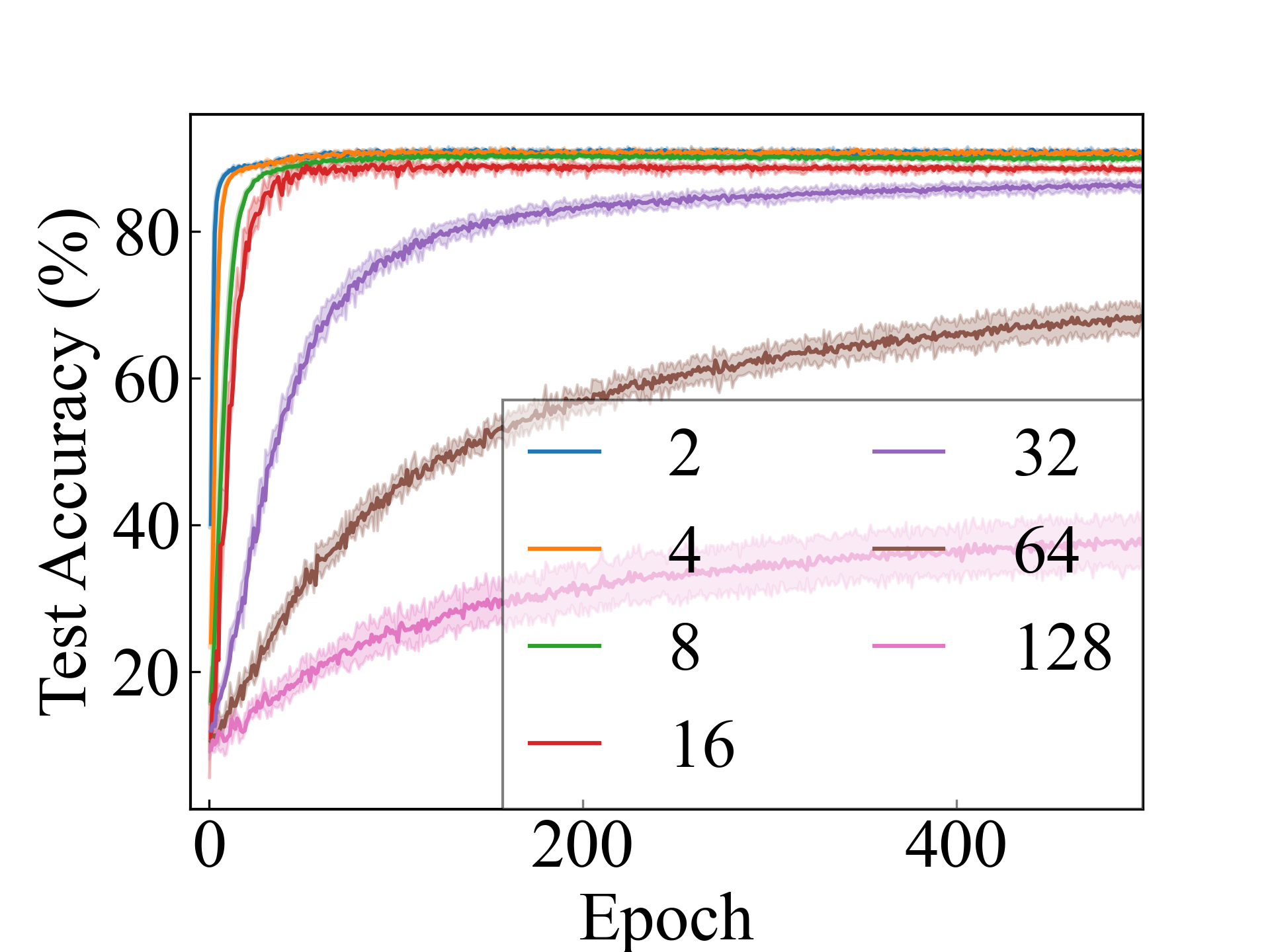
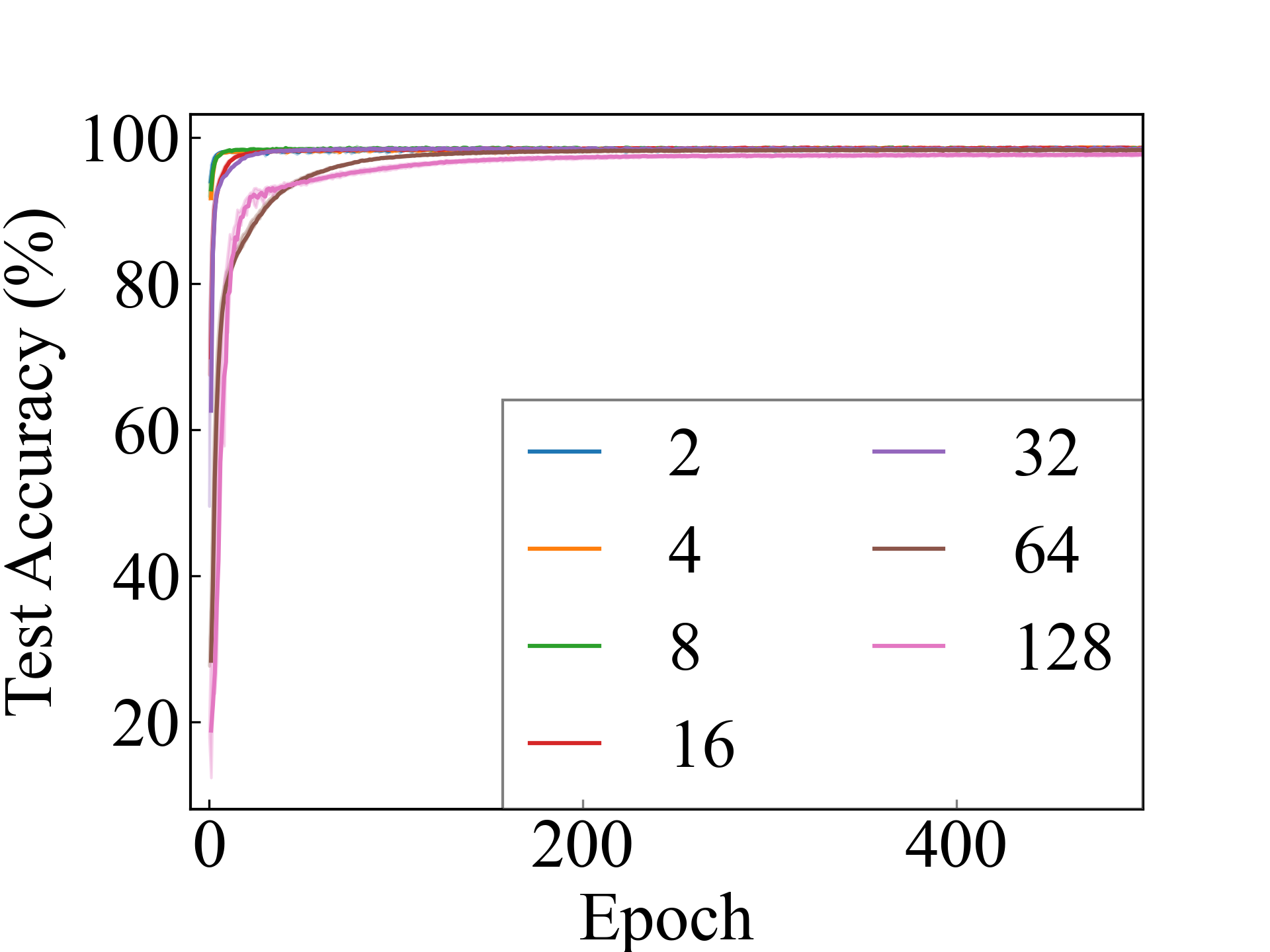
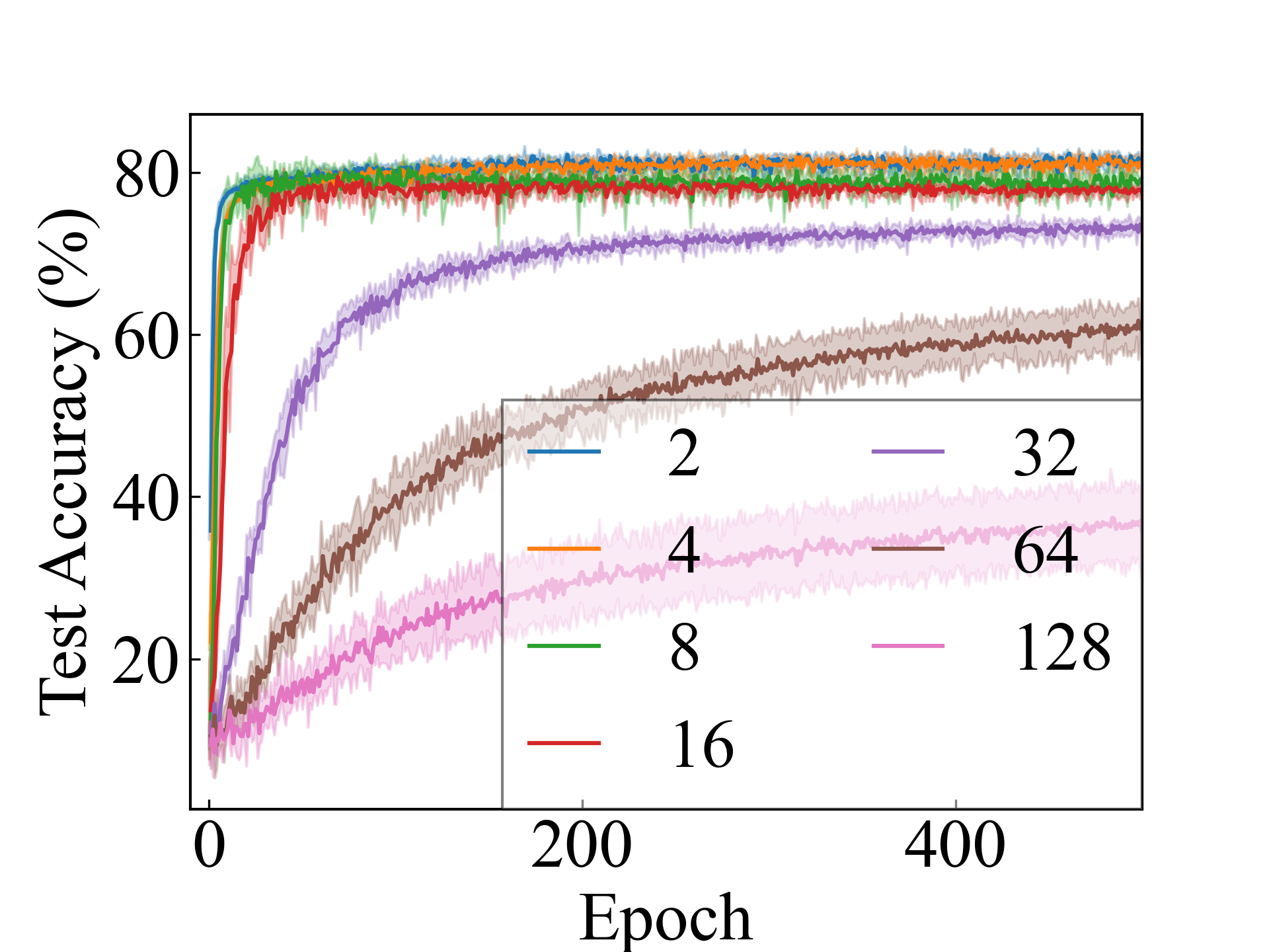
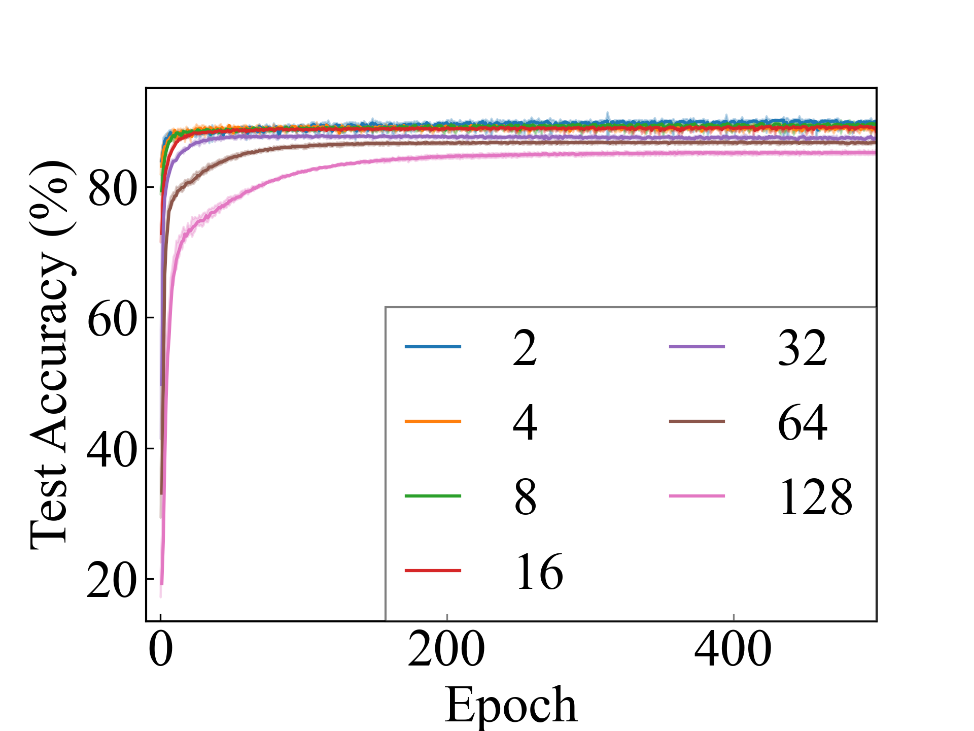
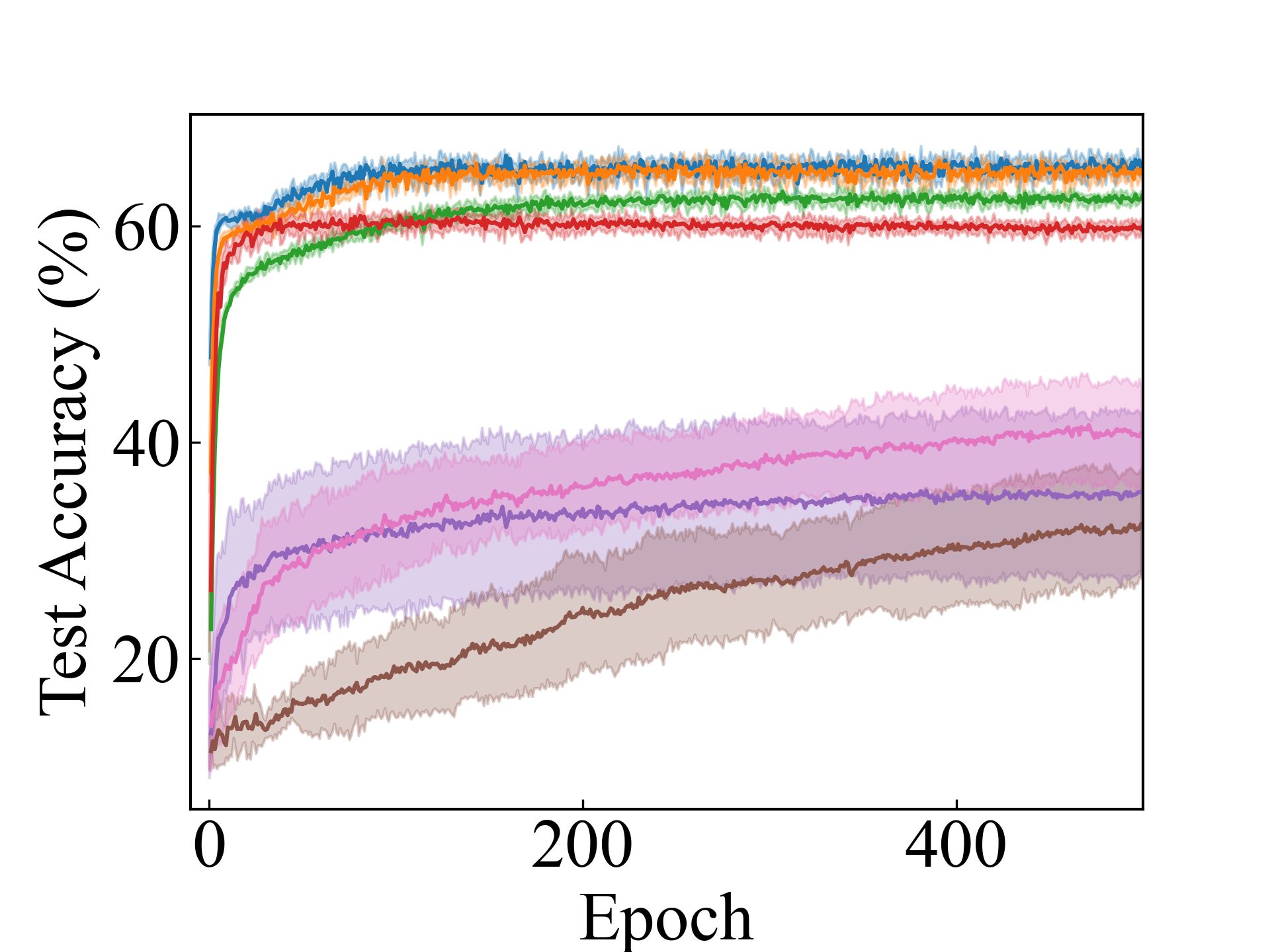
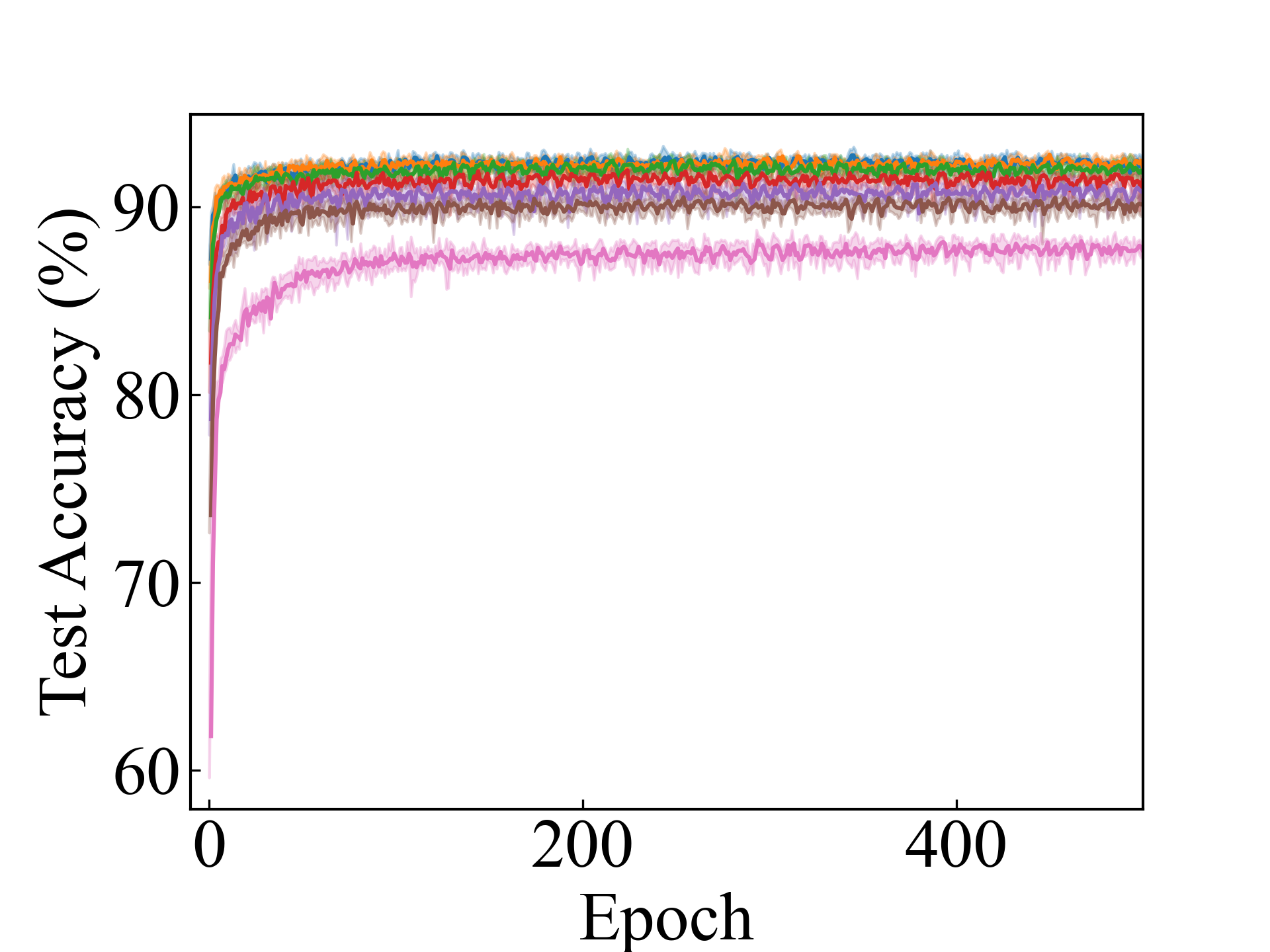
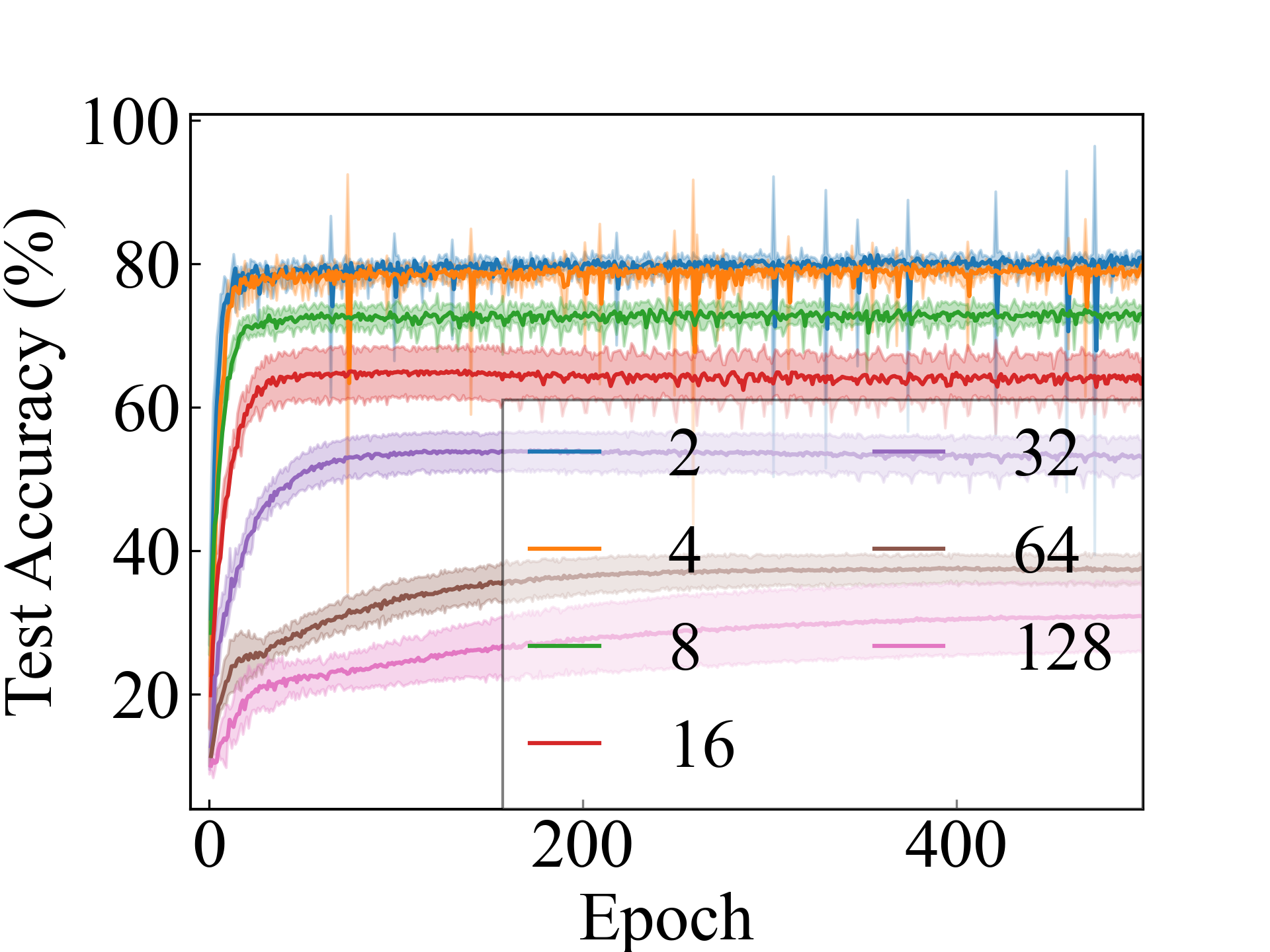
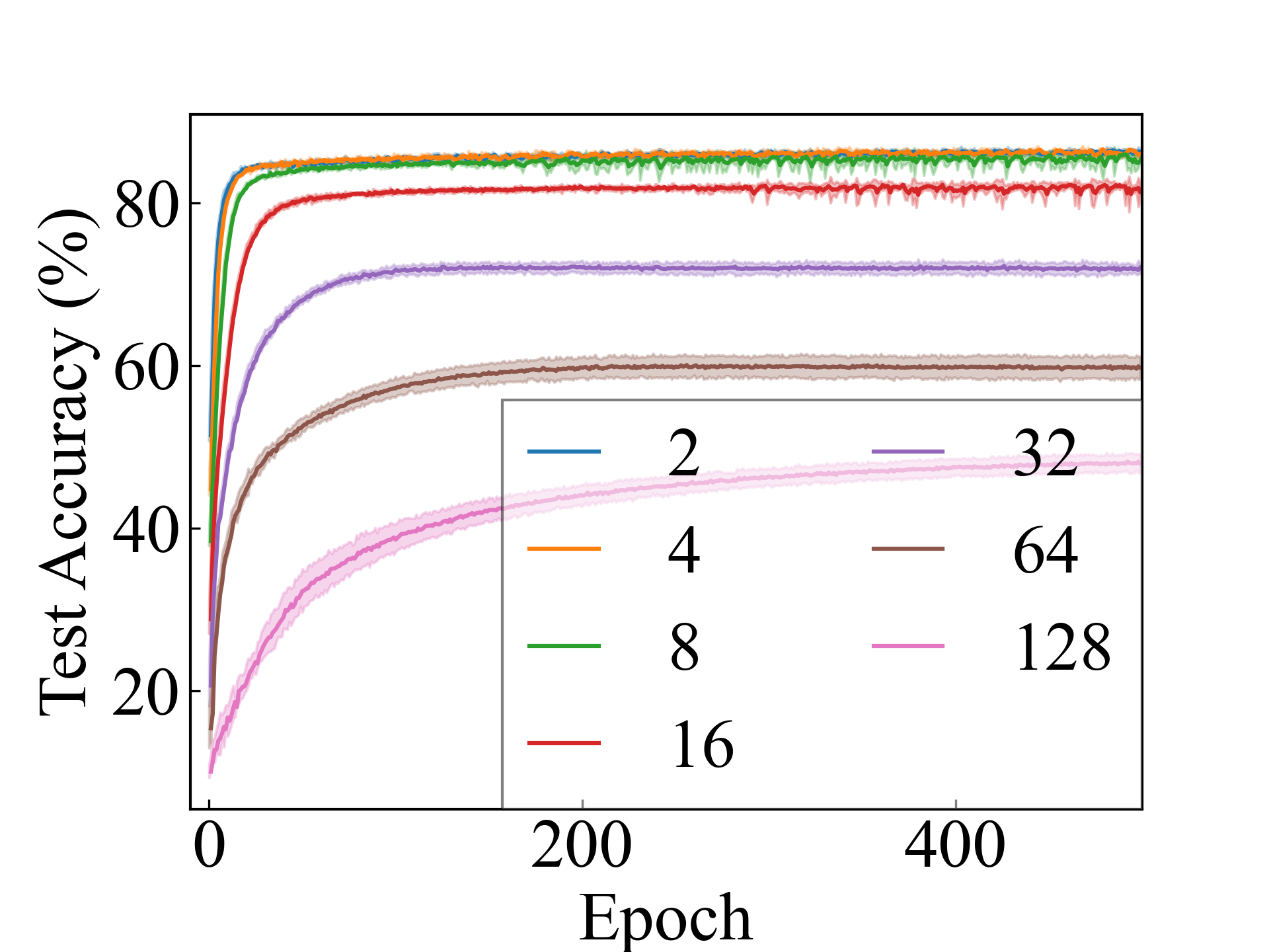
Results The accuracy of the test data was presented in Table 2–4 and 1. We also report the paired $t$ -test results at a $5\%$ significance level for the best of the proposed methods and each comparison method. $\bullet$ and $\circ$ indicate that our best method was significantly better and worse, respectively.

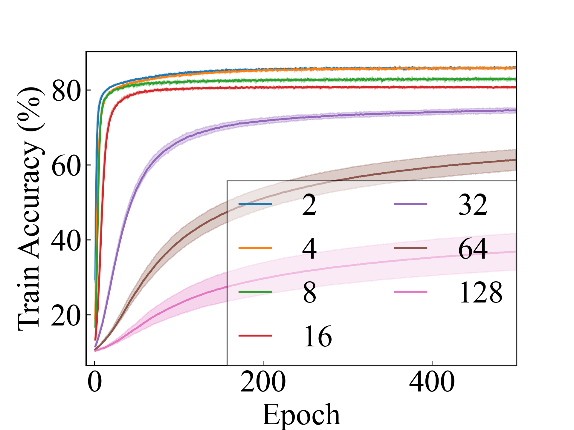
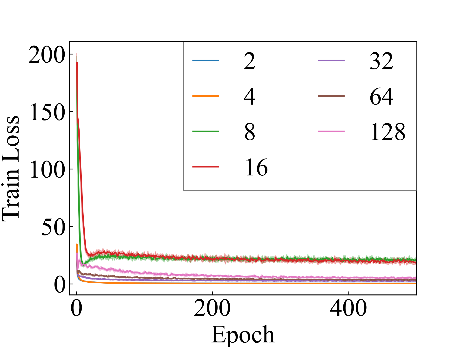
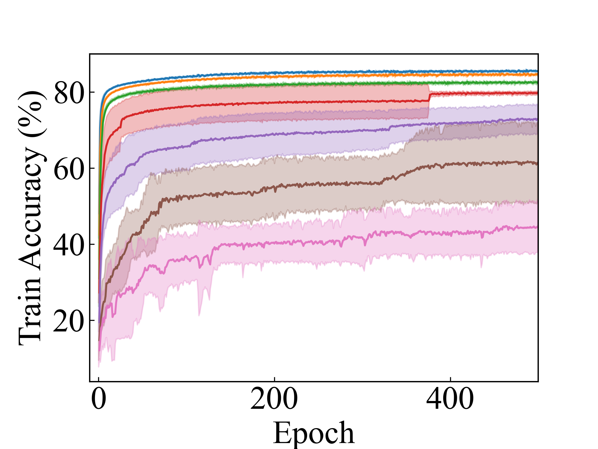
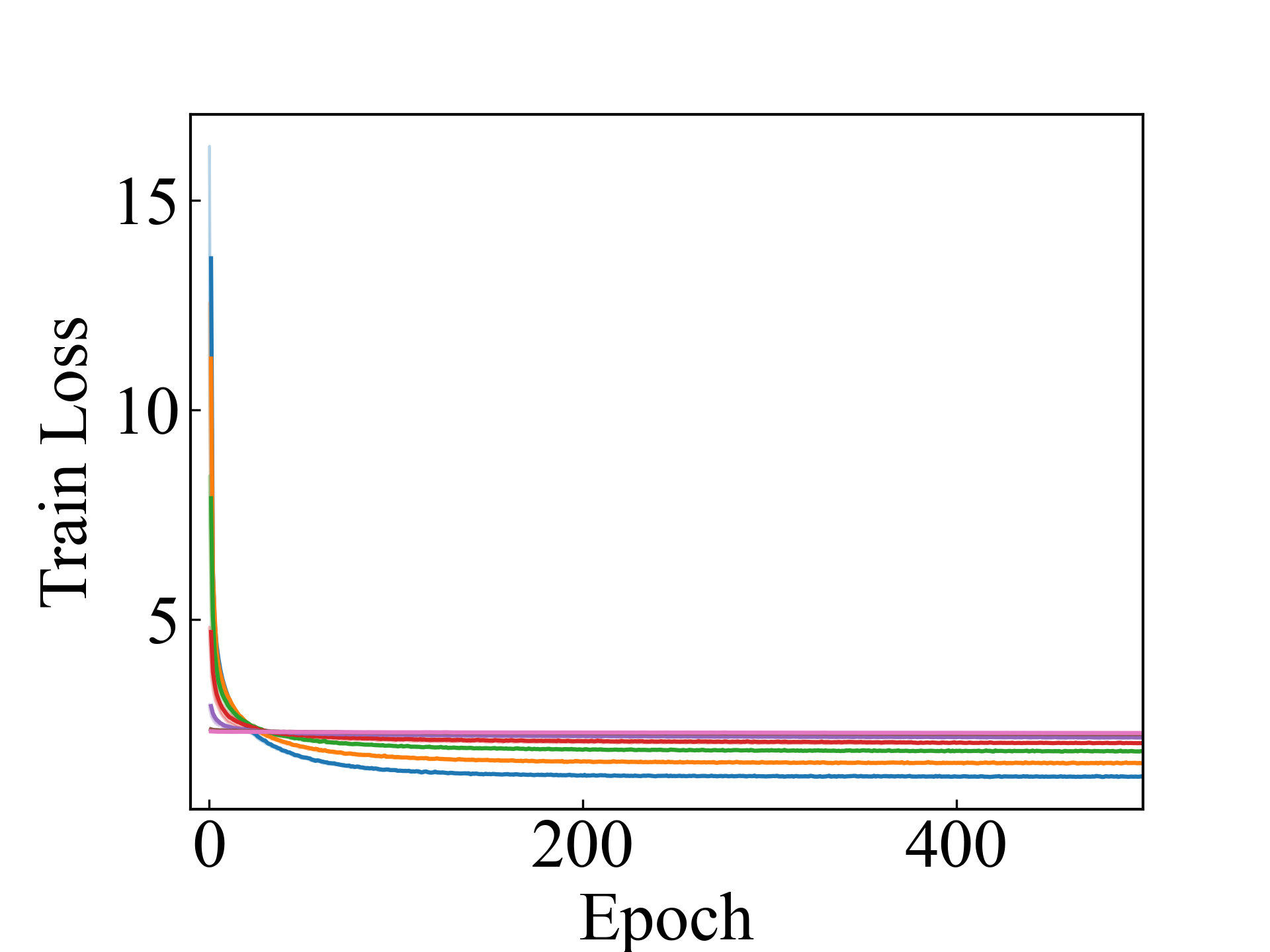
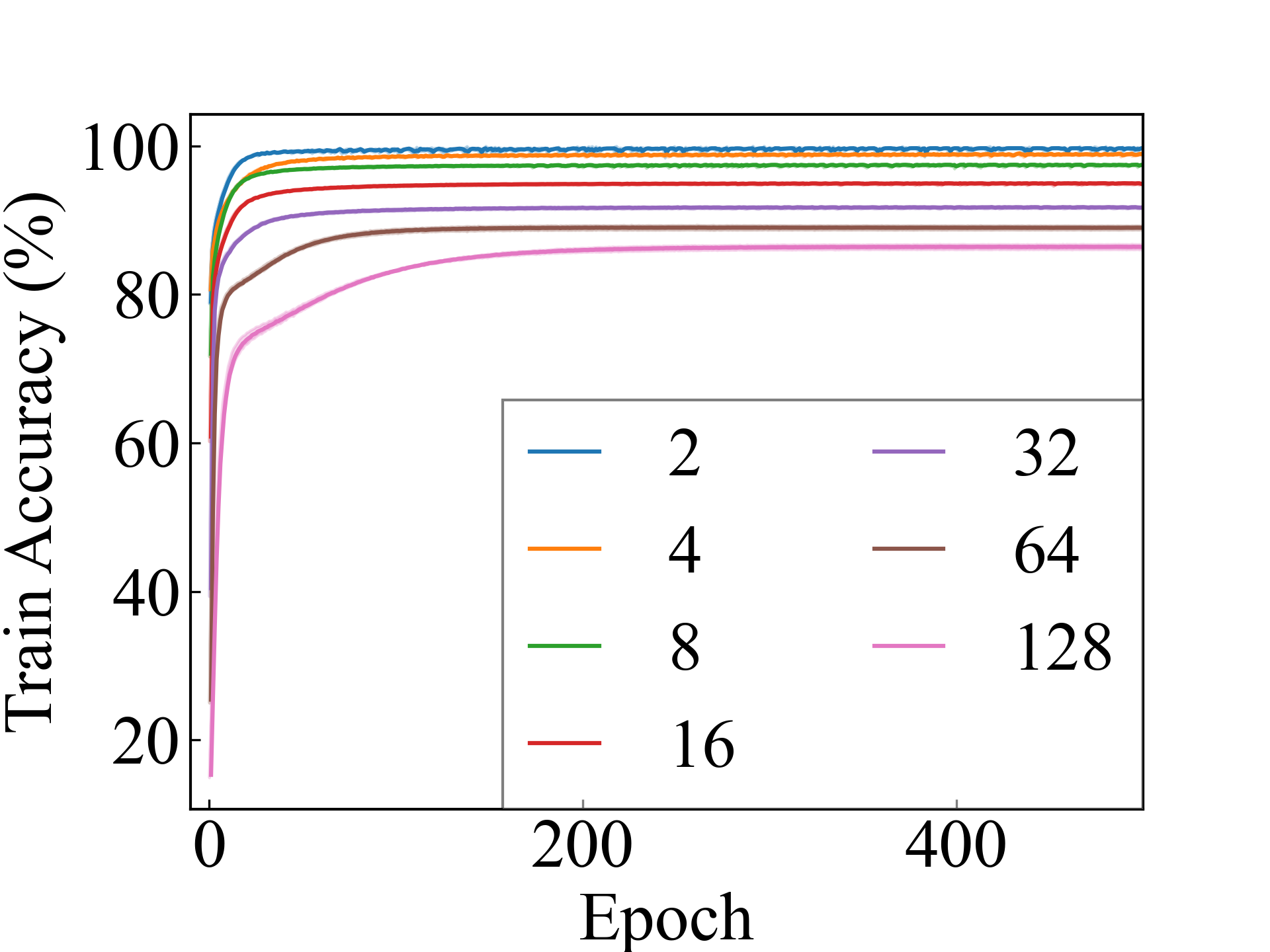
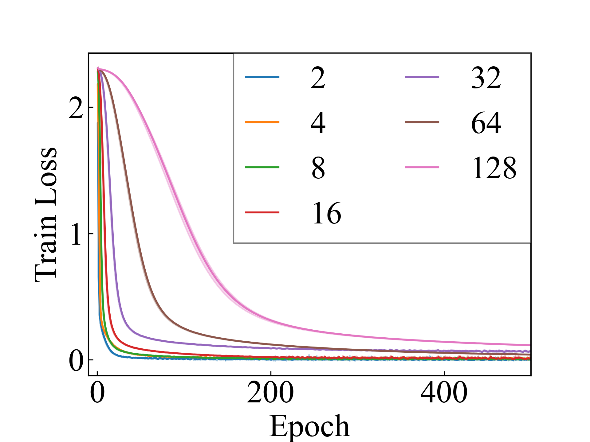
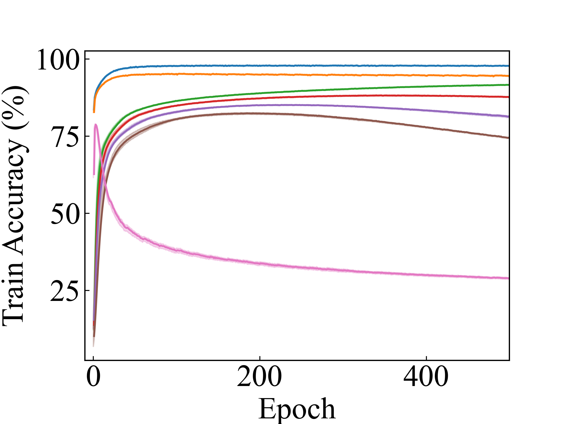
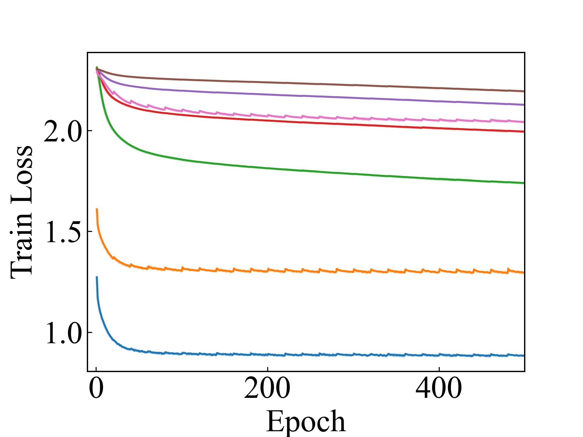
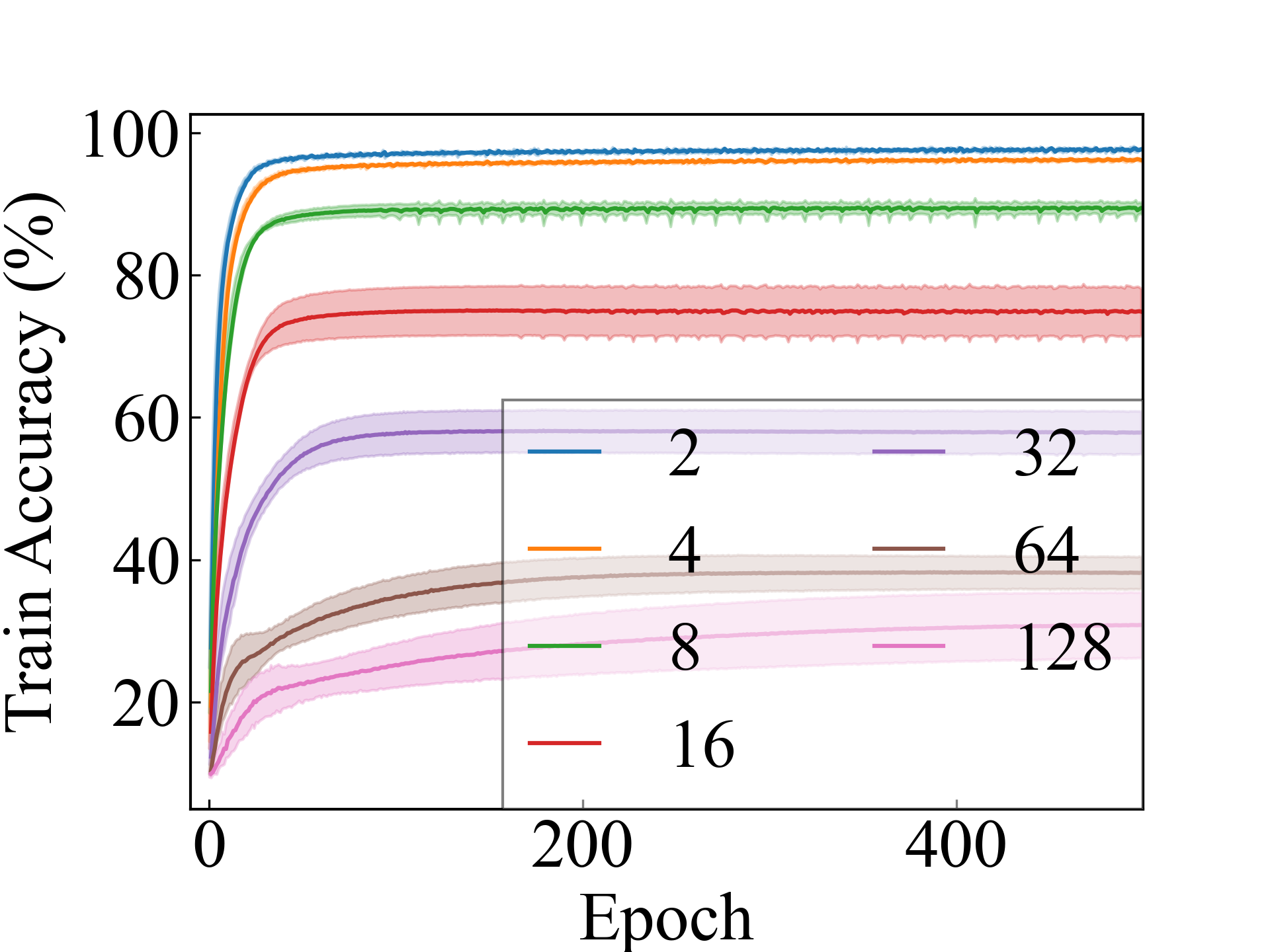
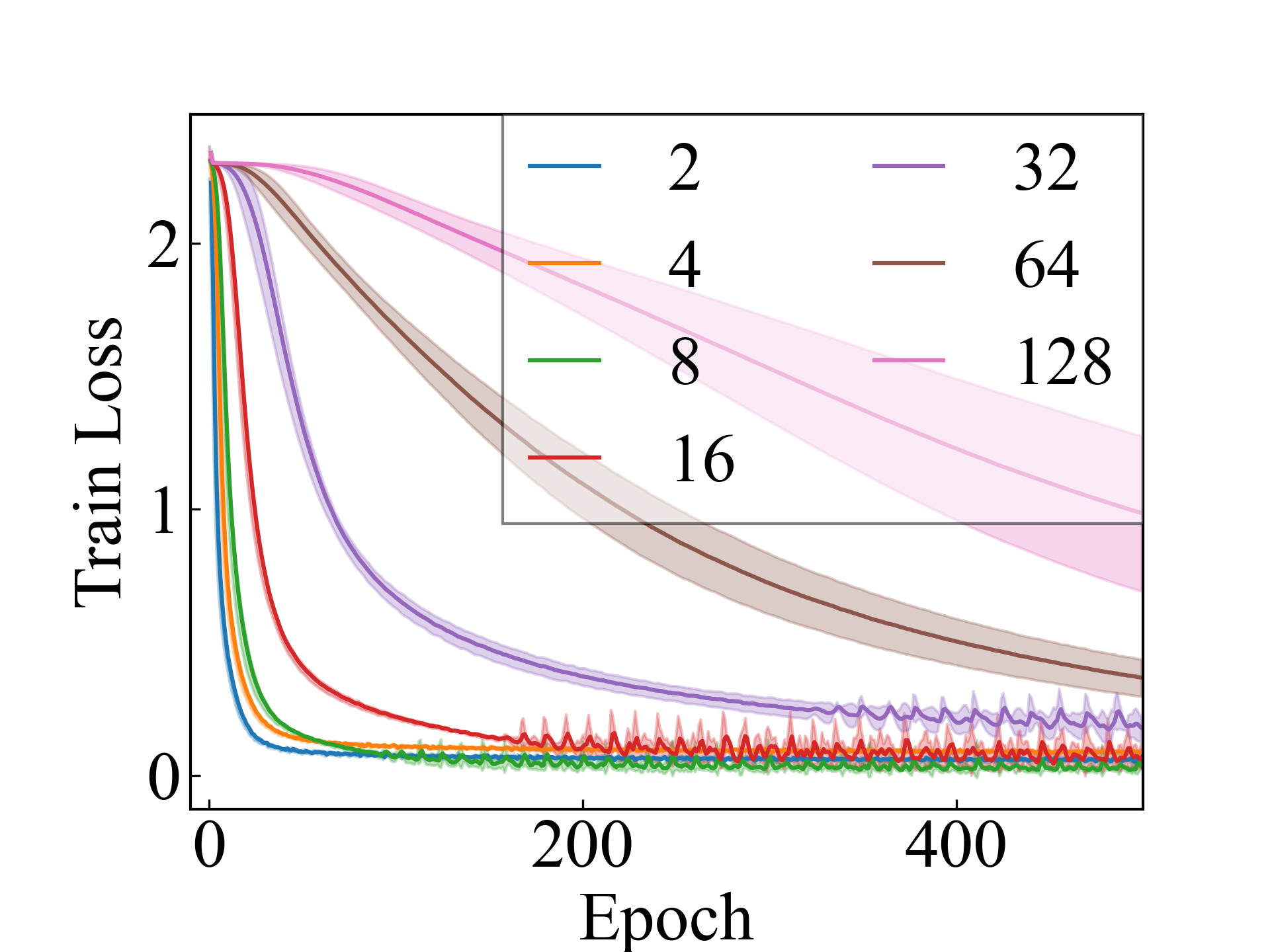
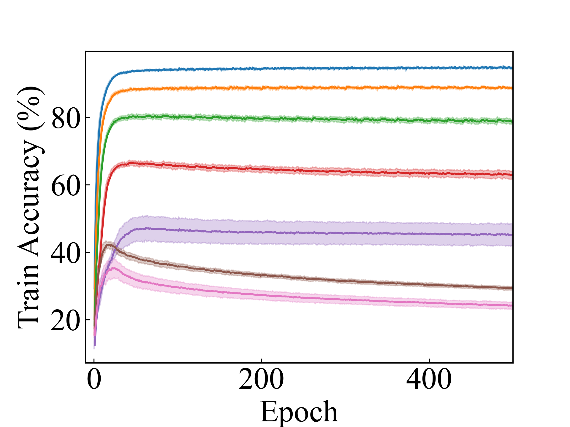
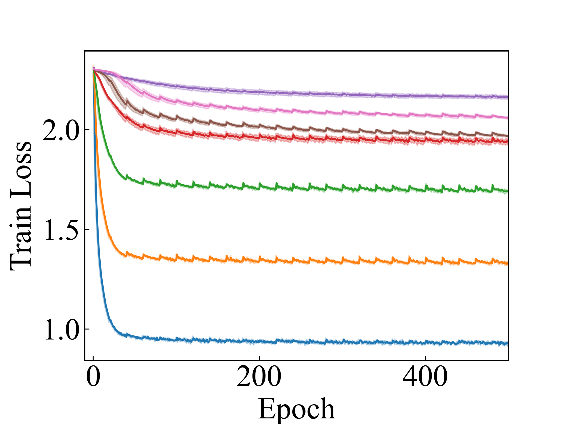
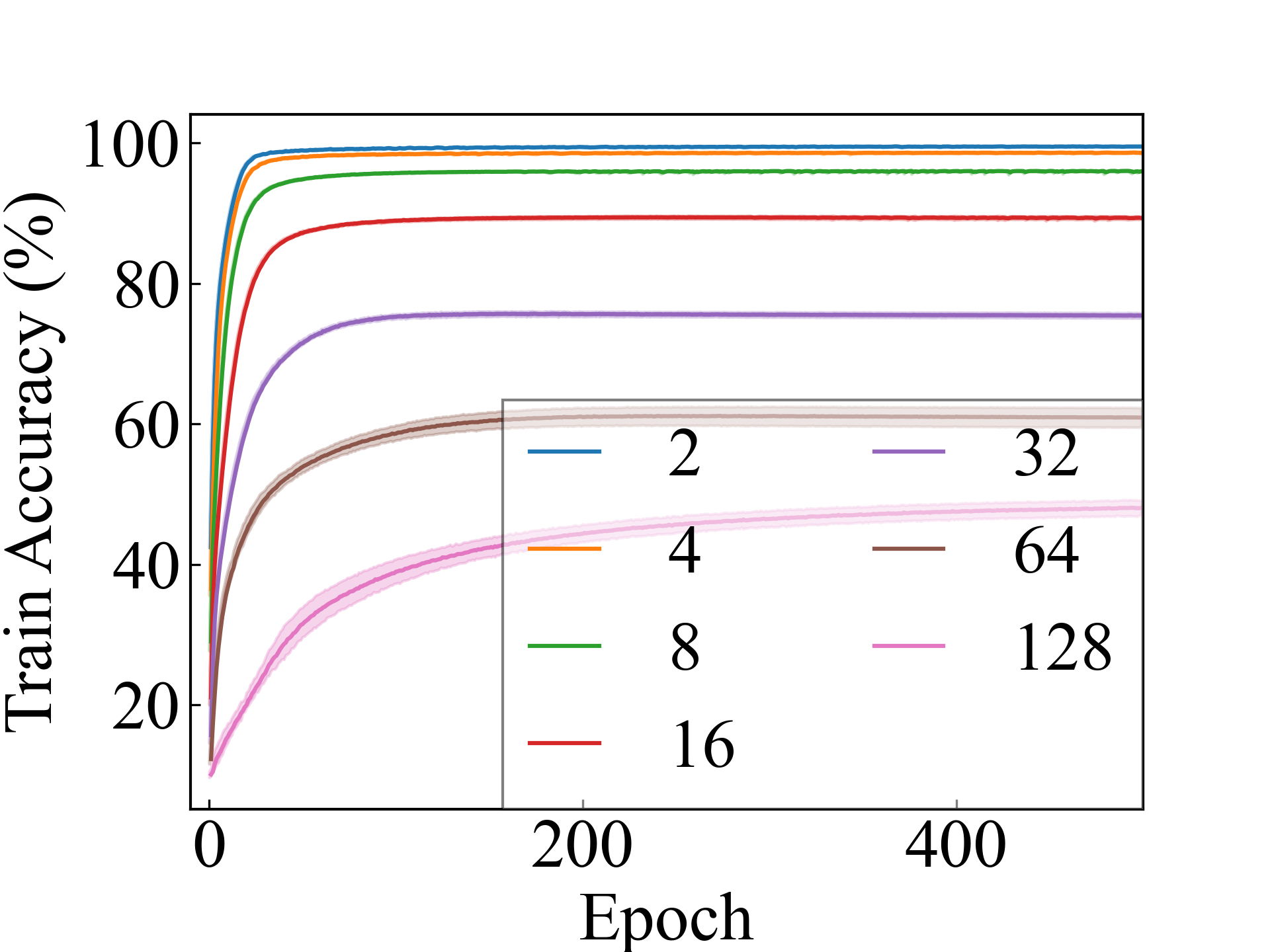
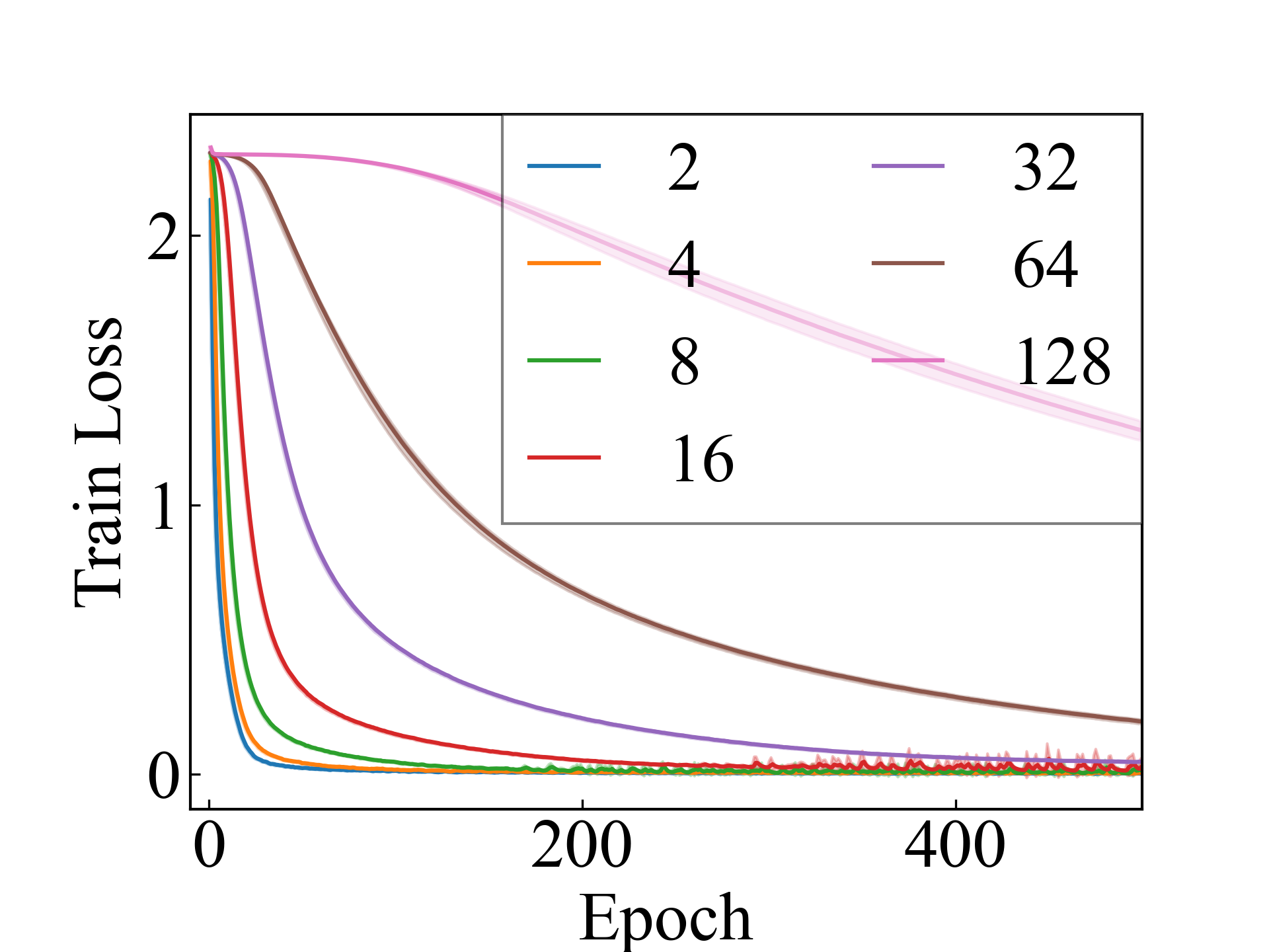
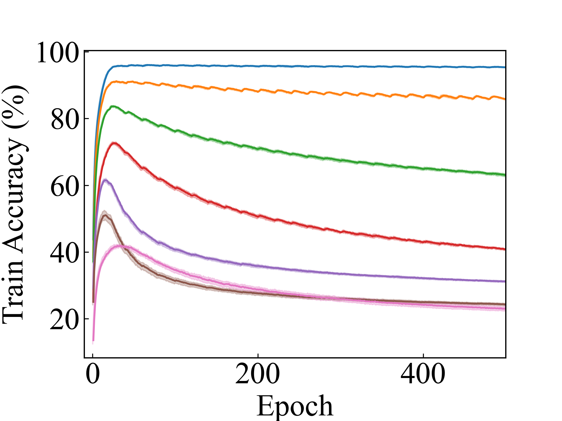
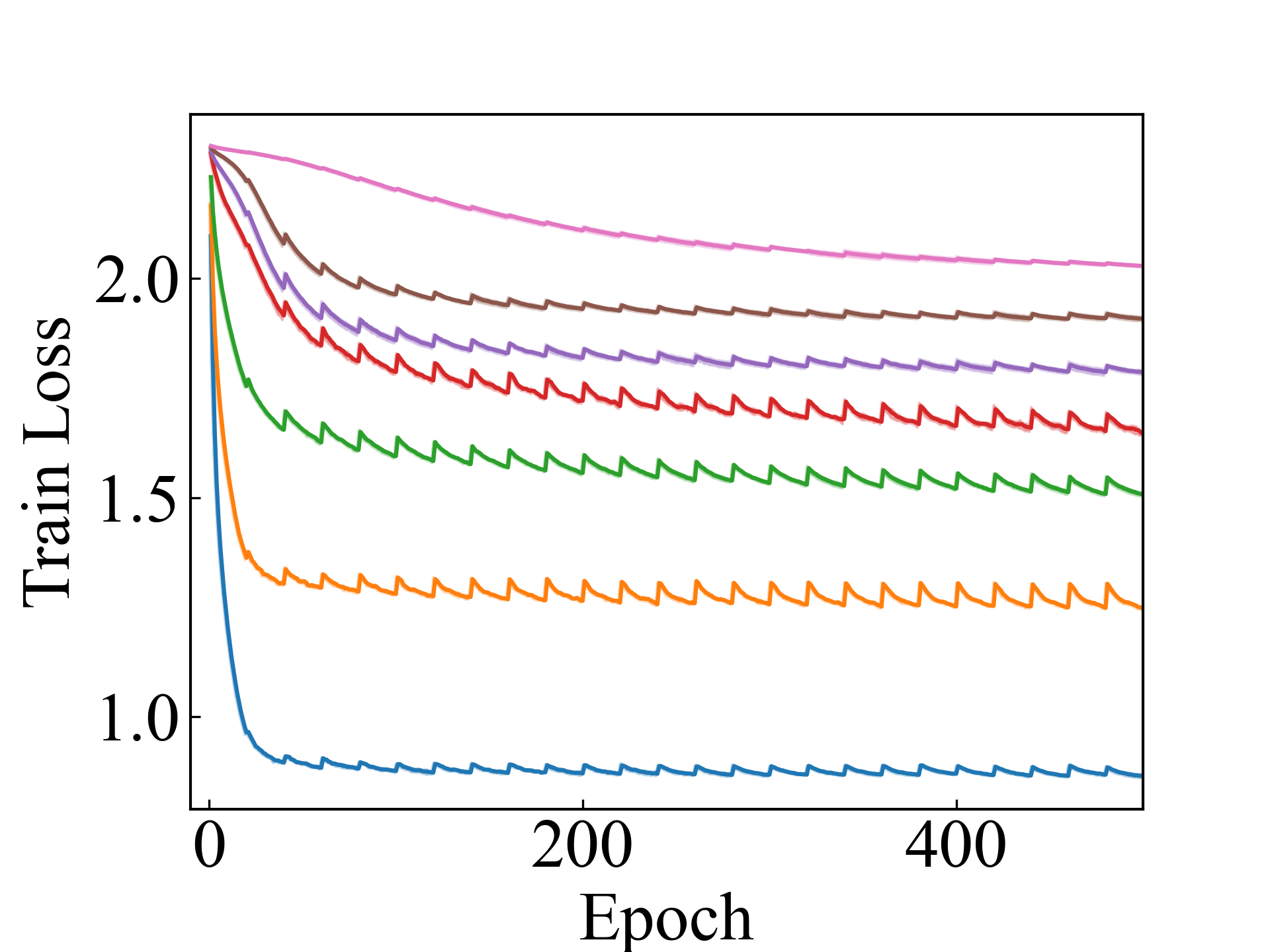
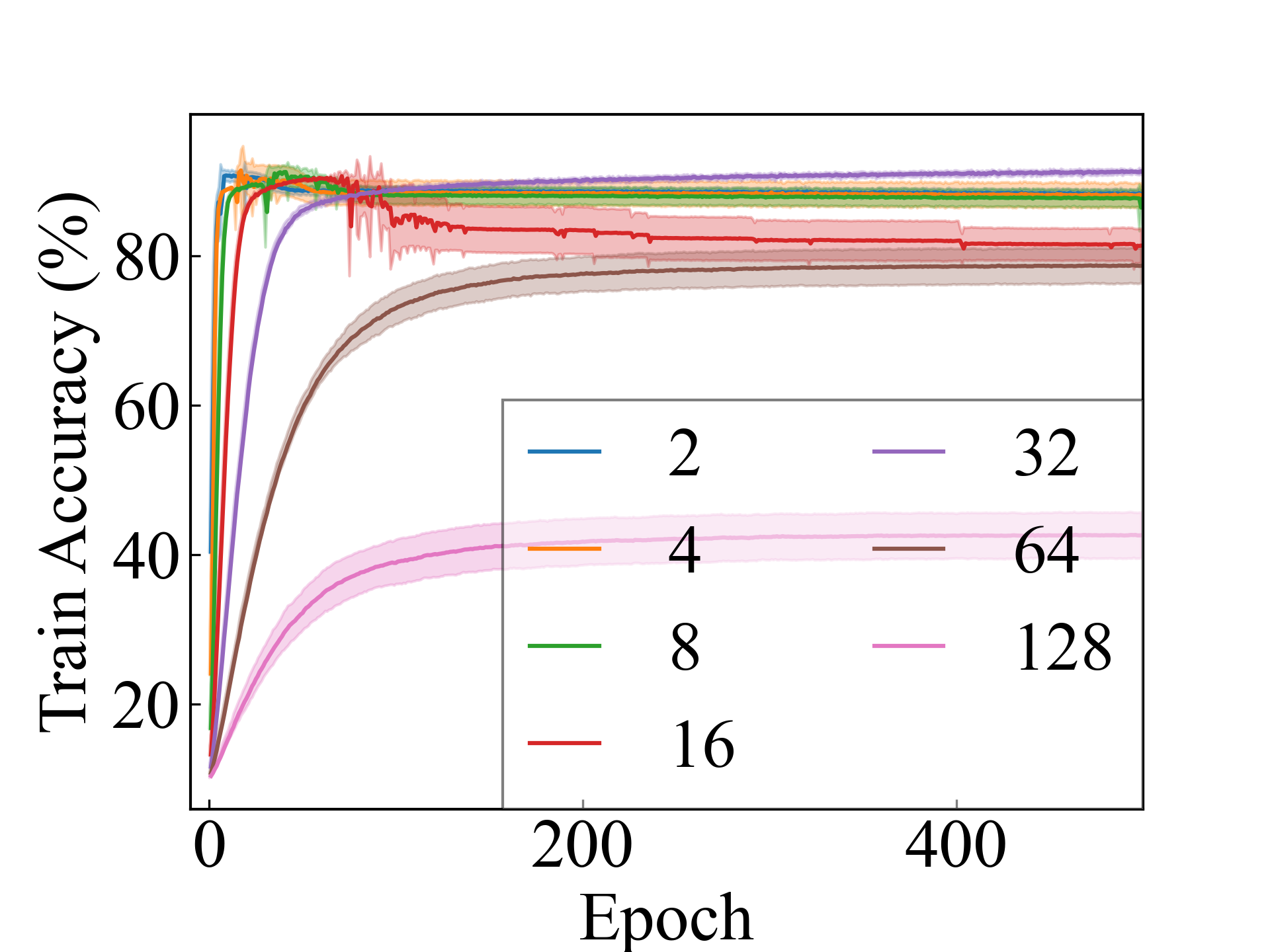
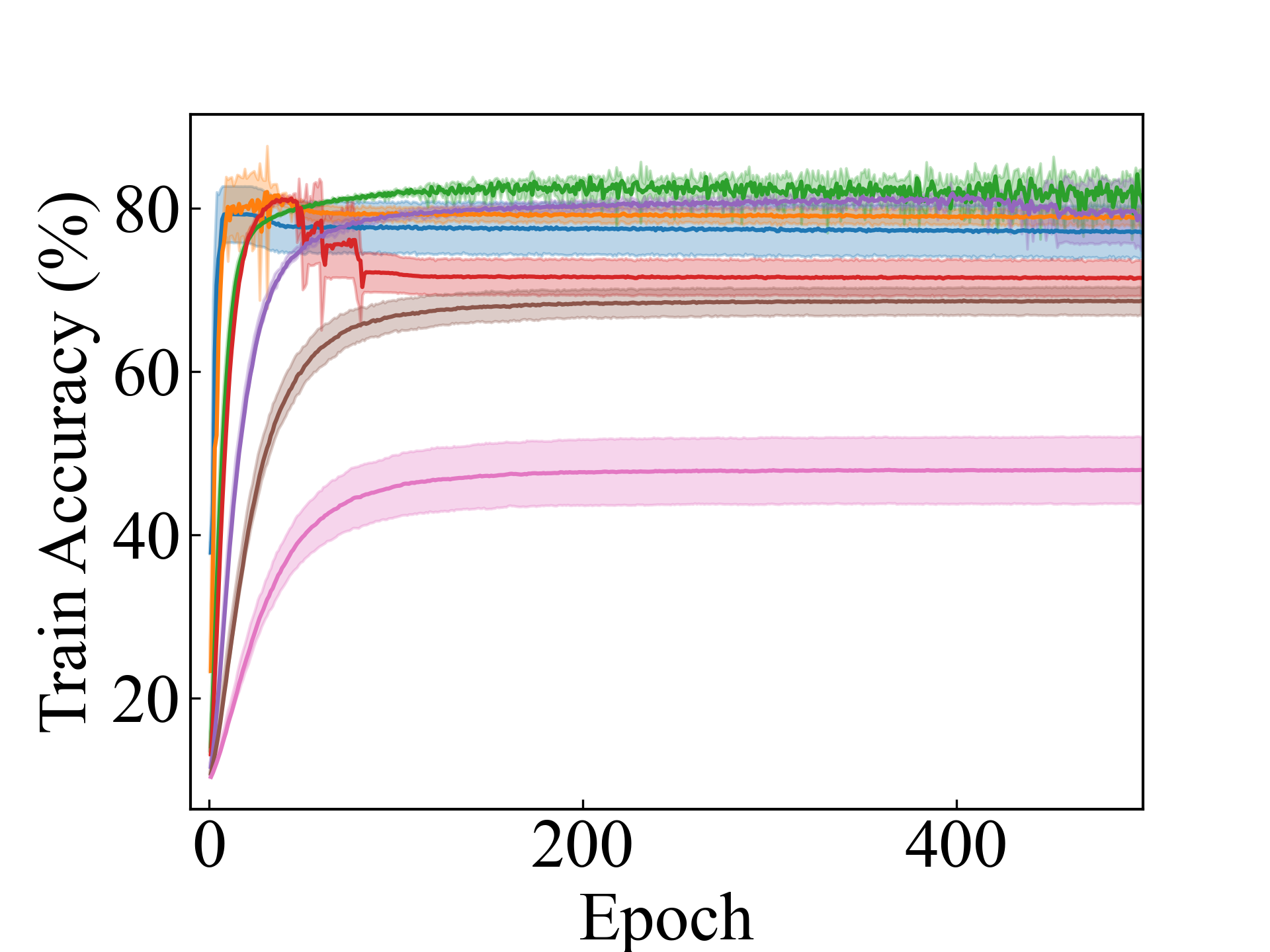
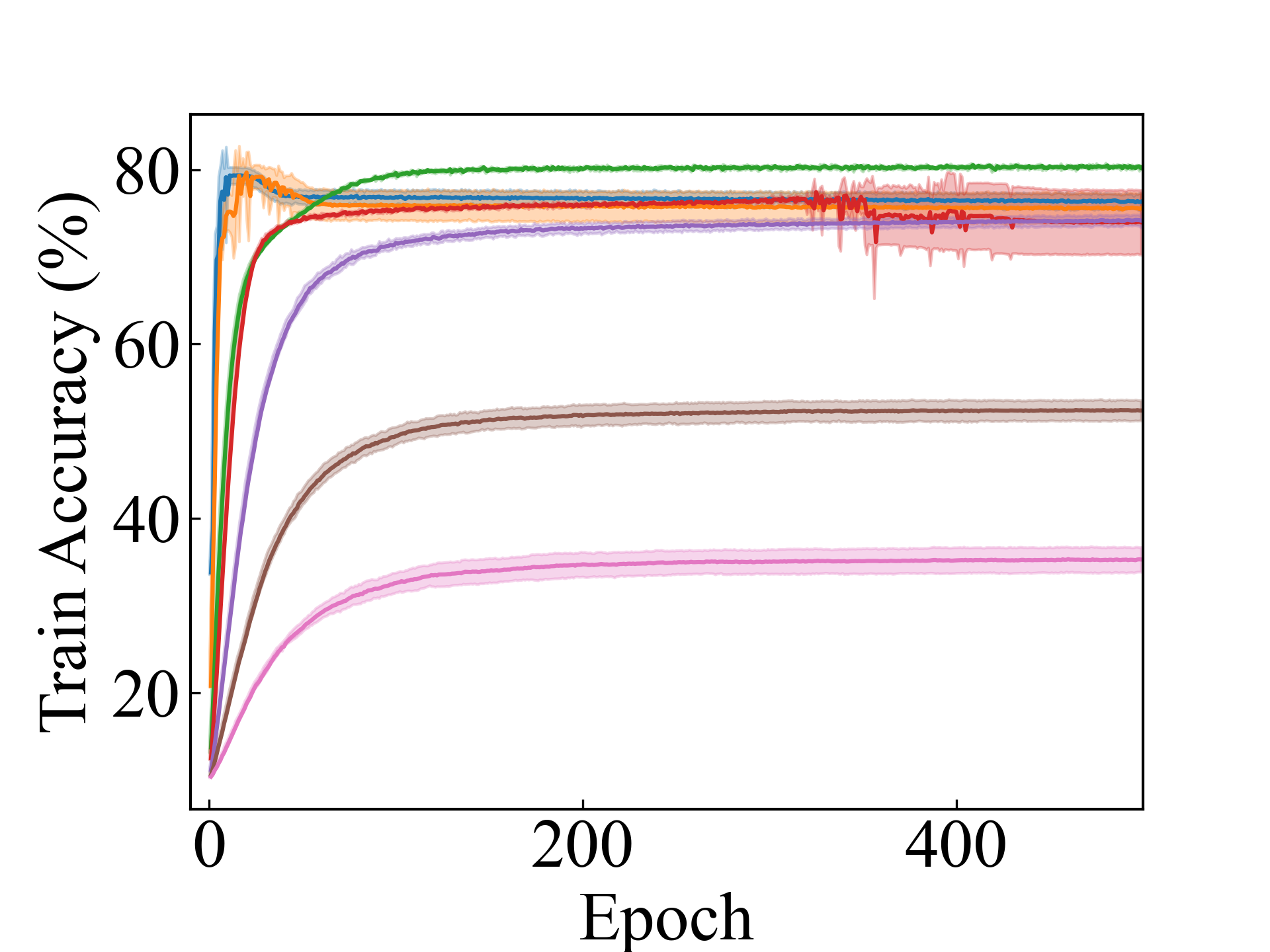
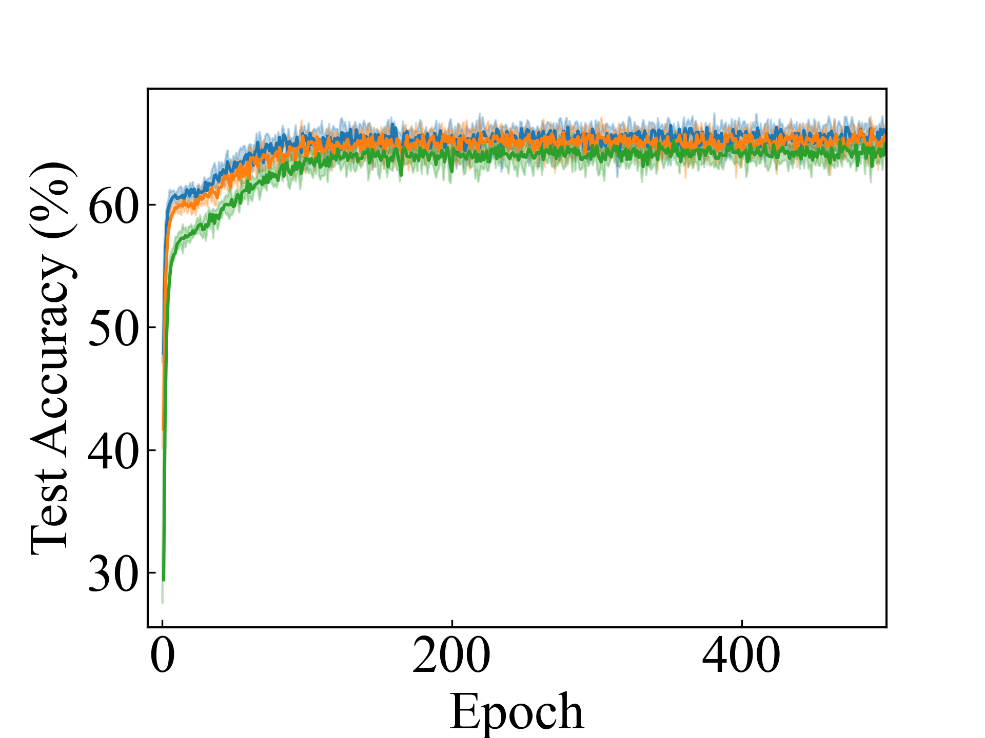
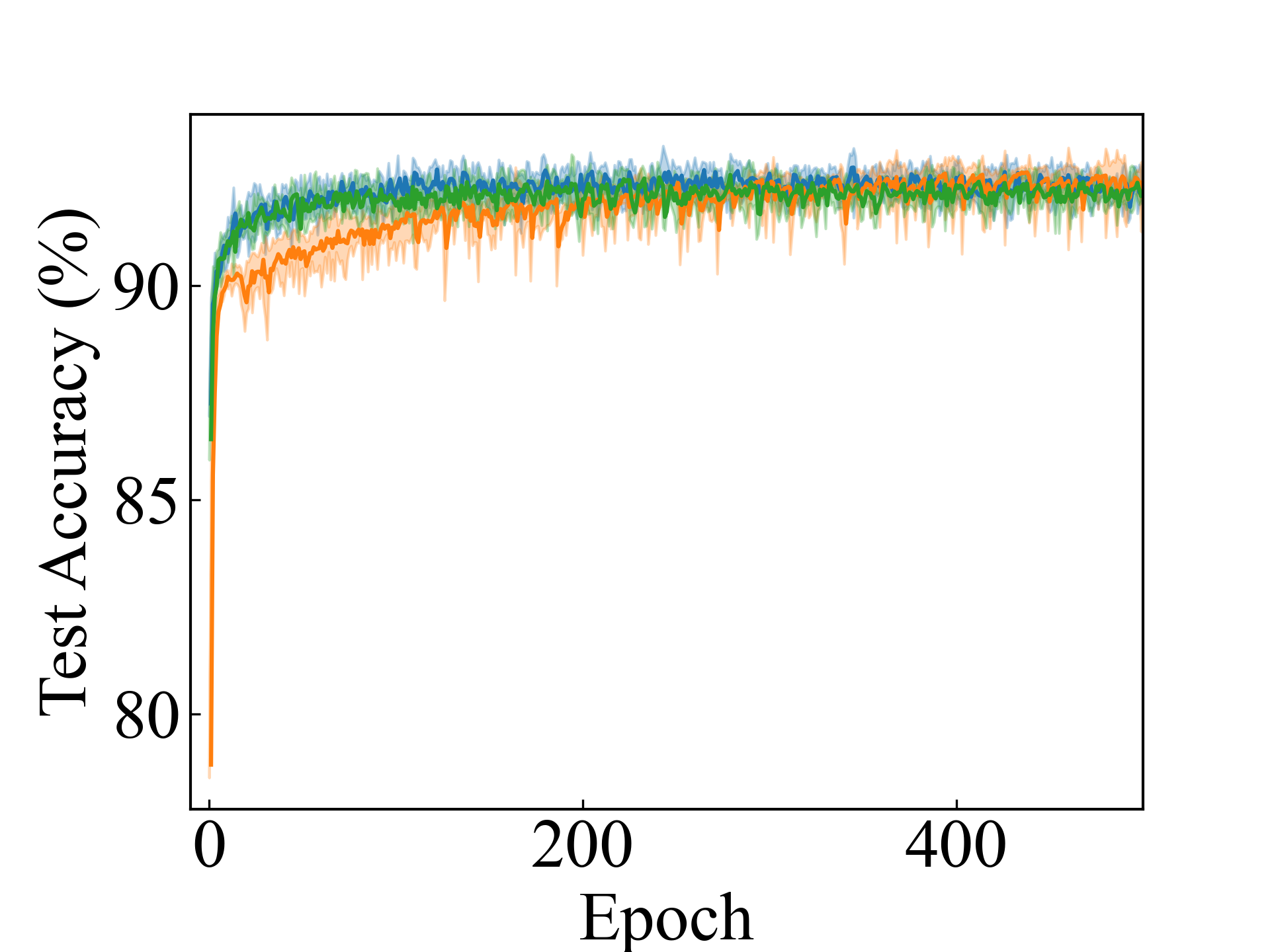
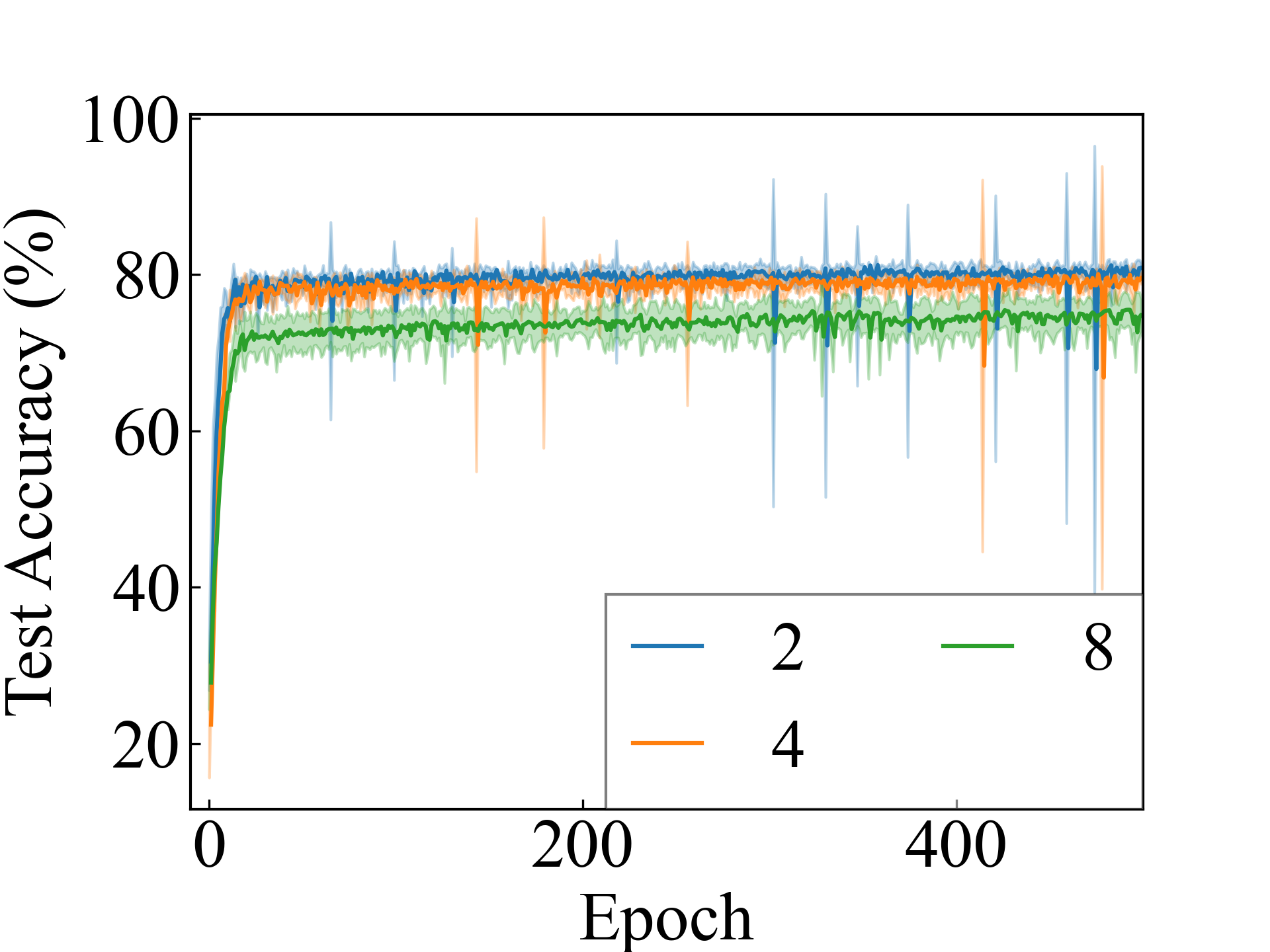
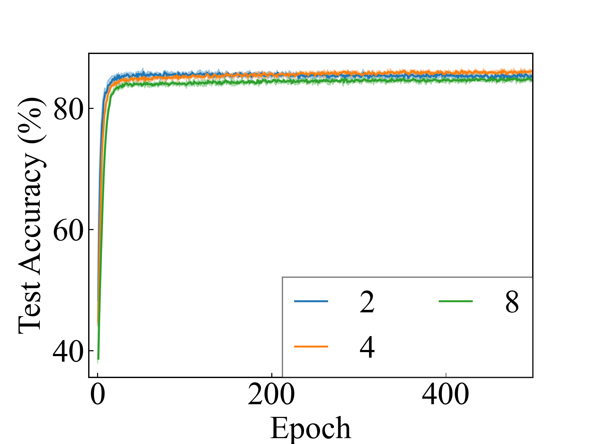
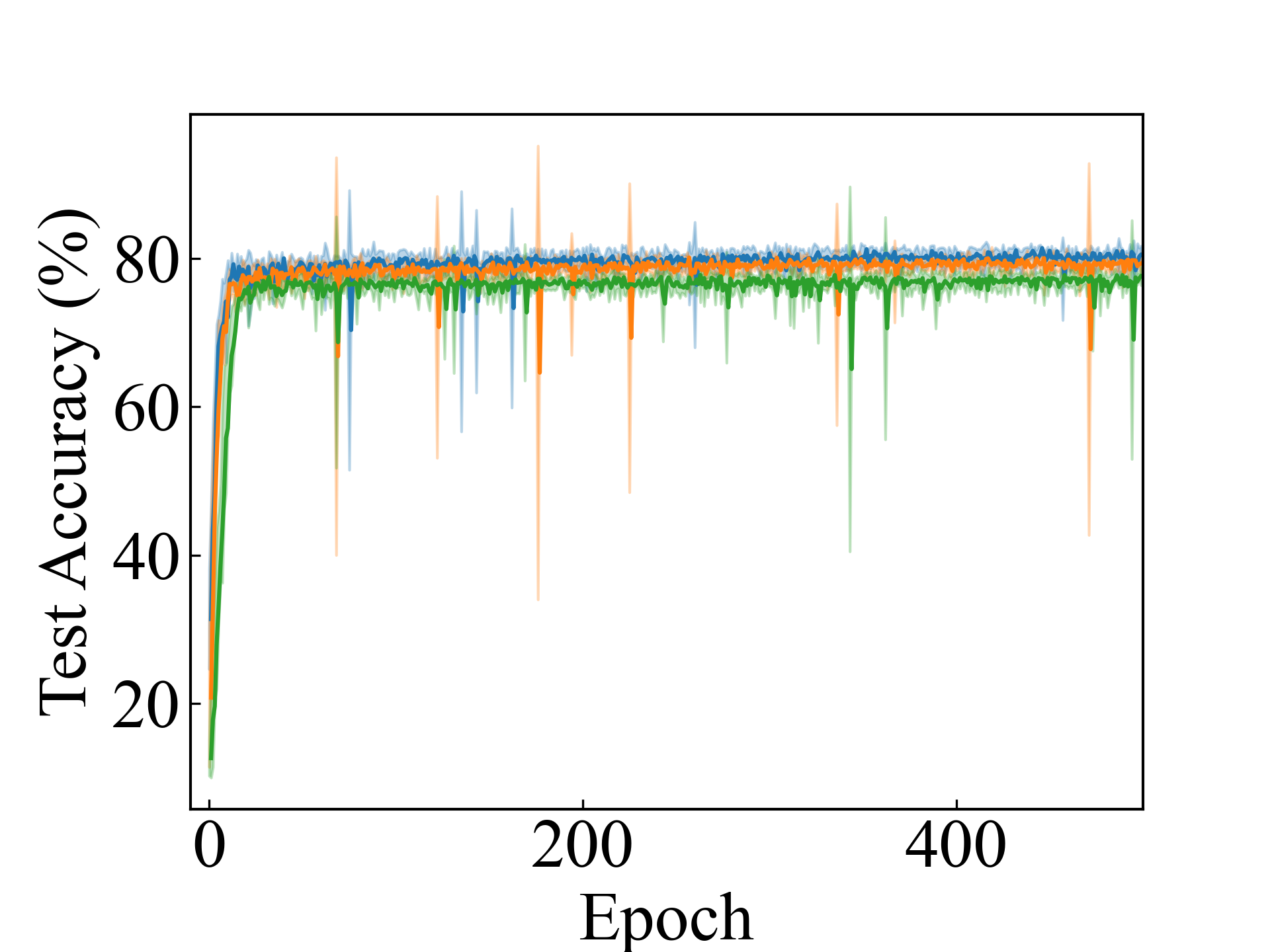
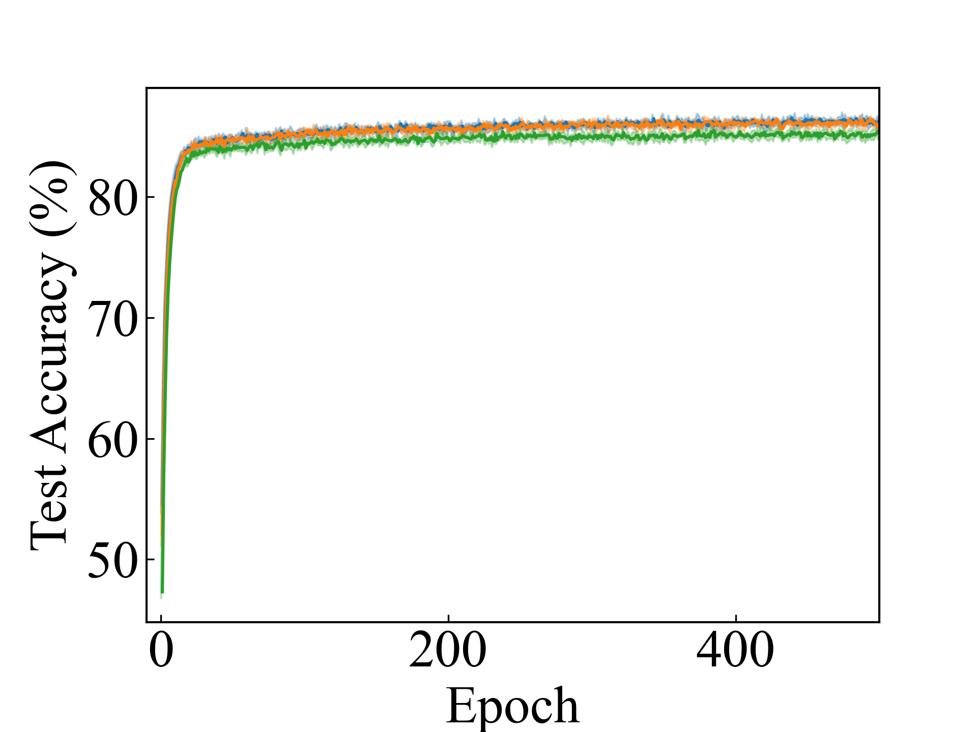
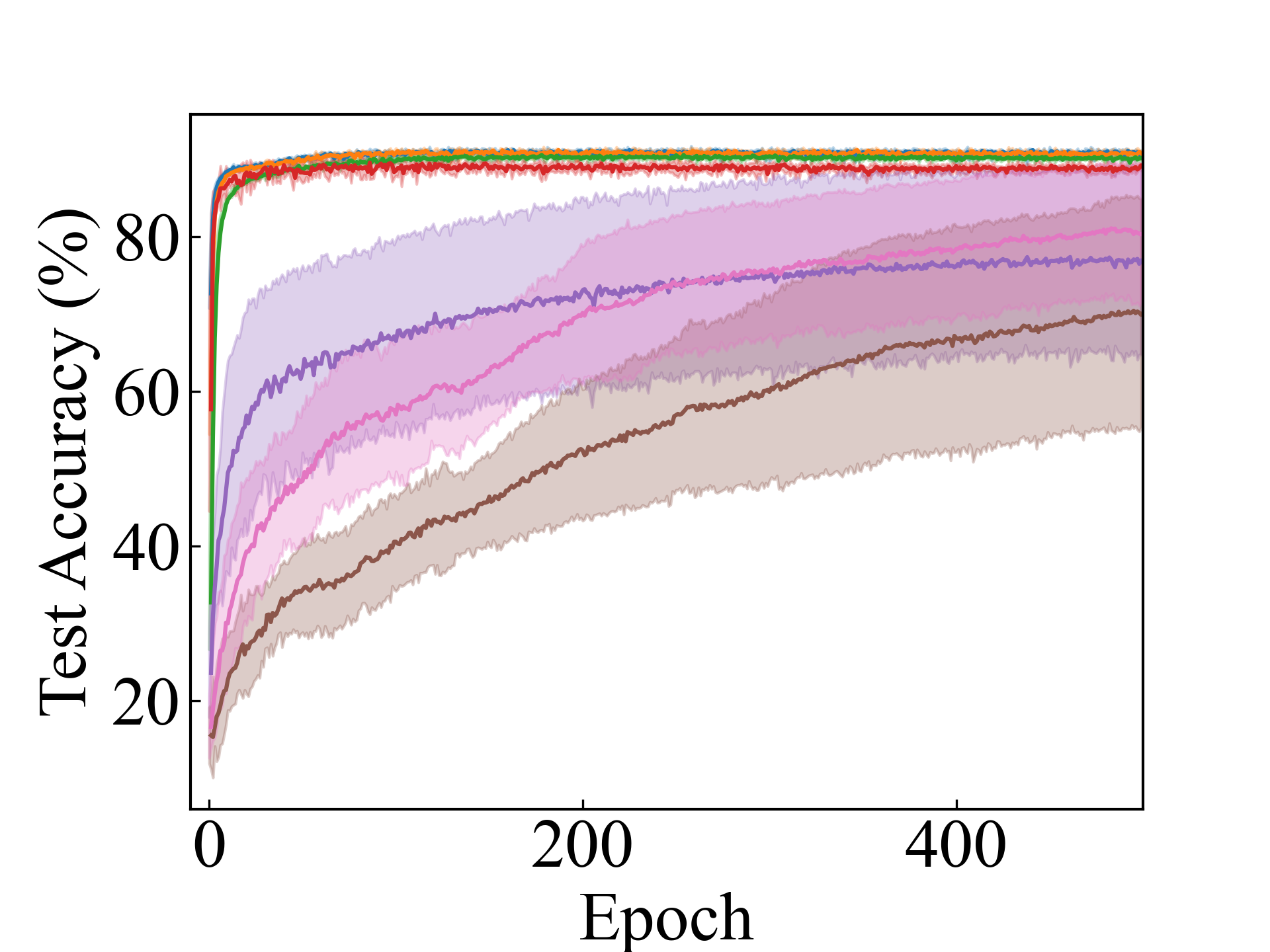
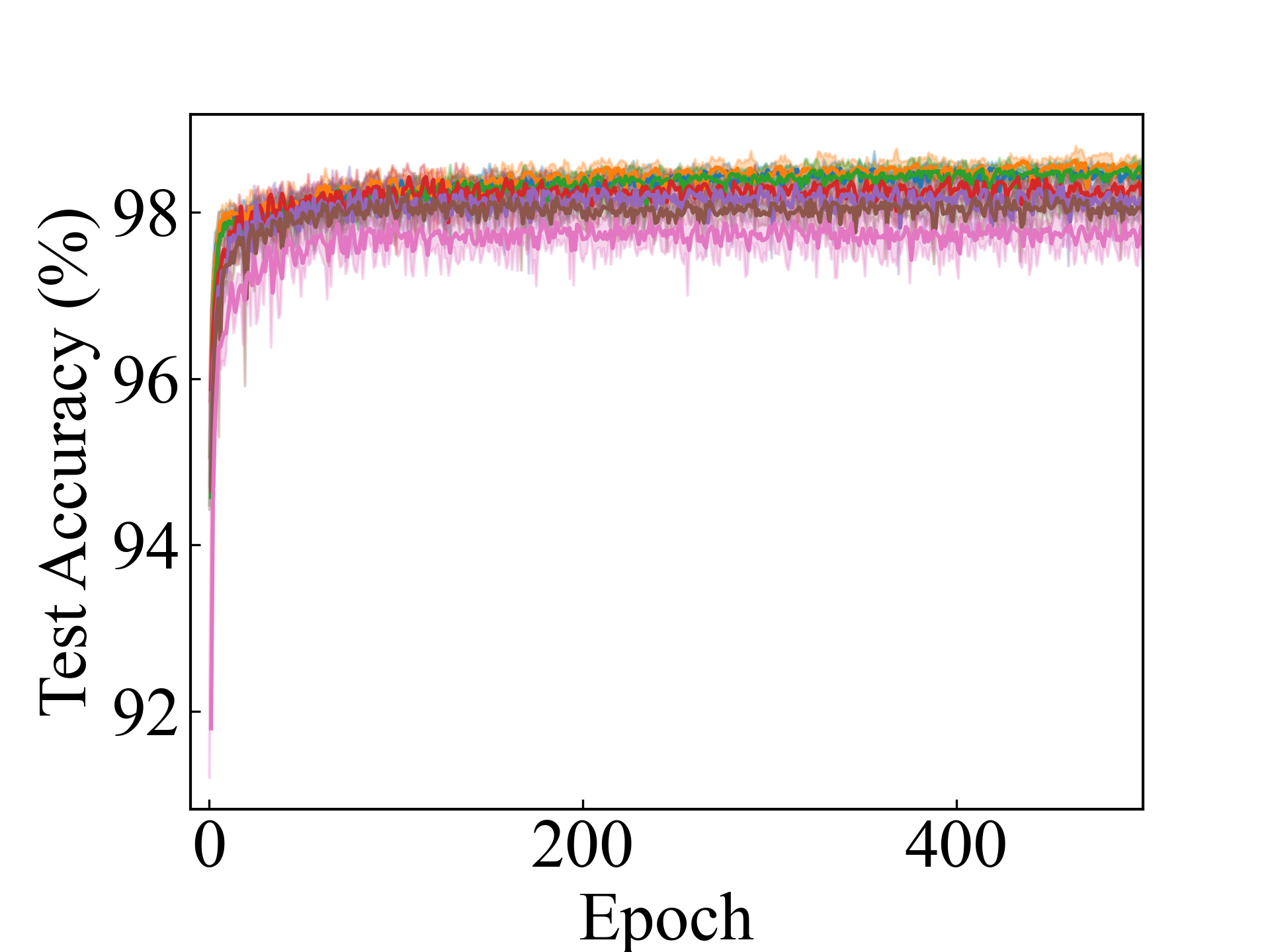
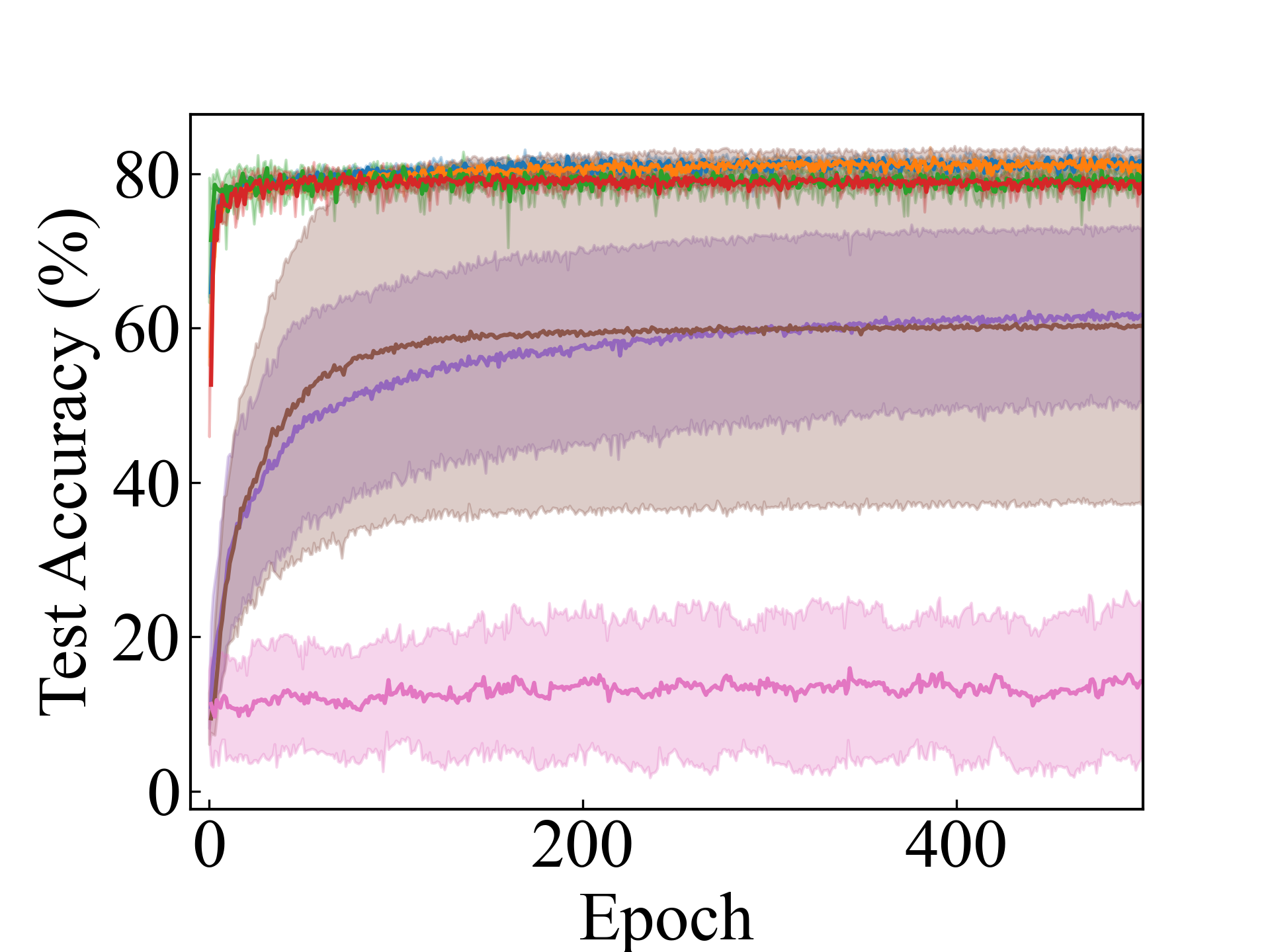
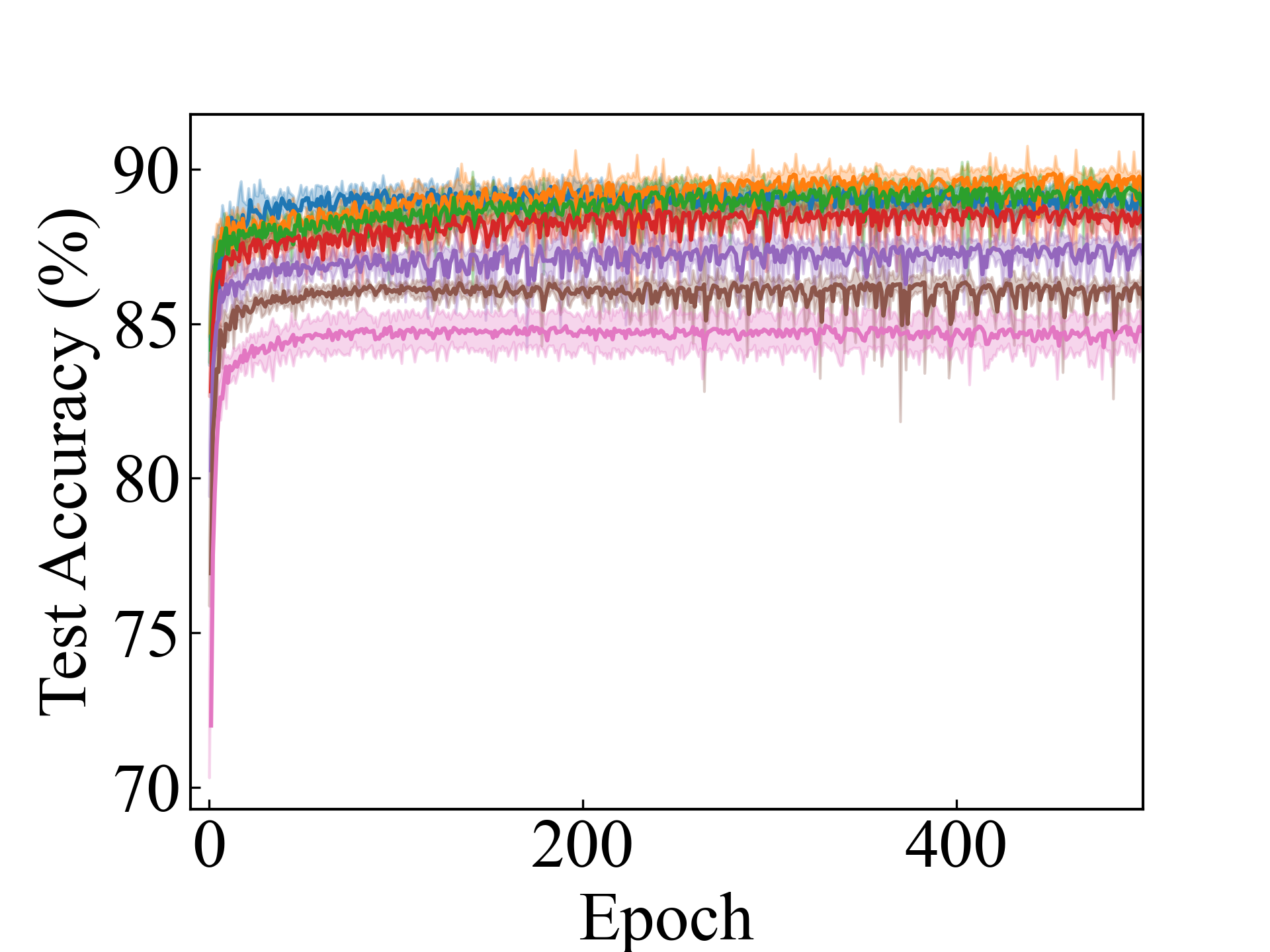
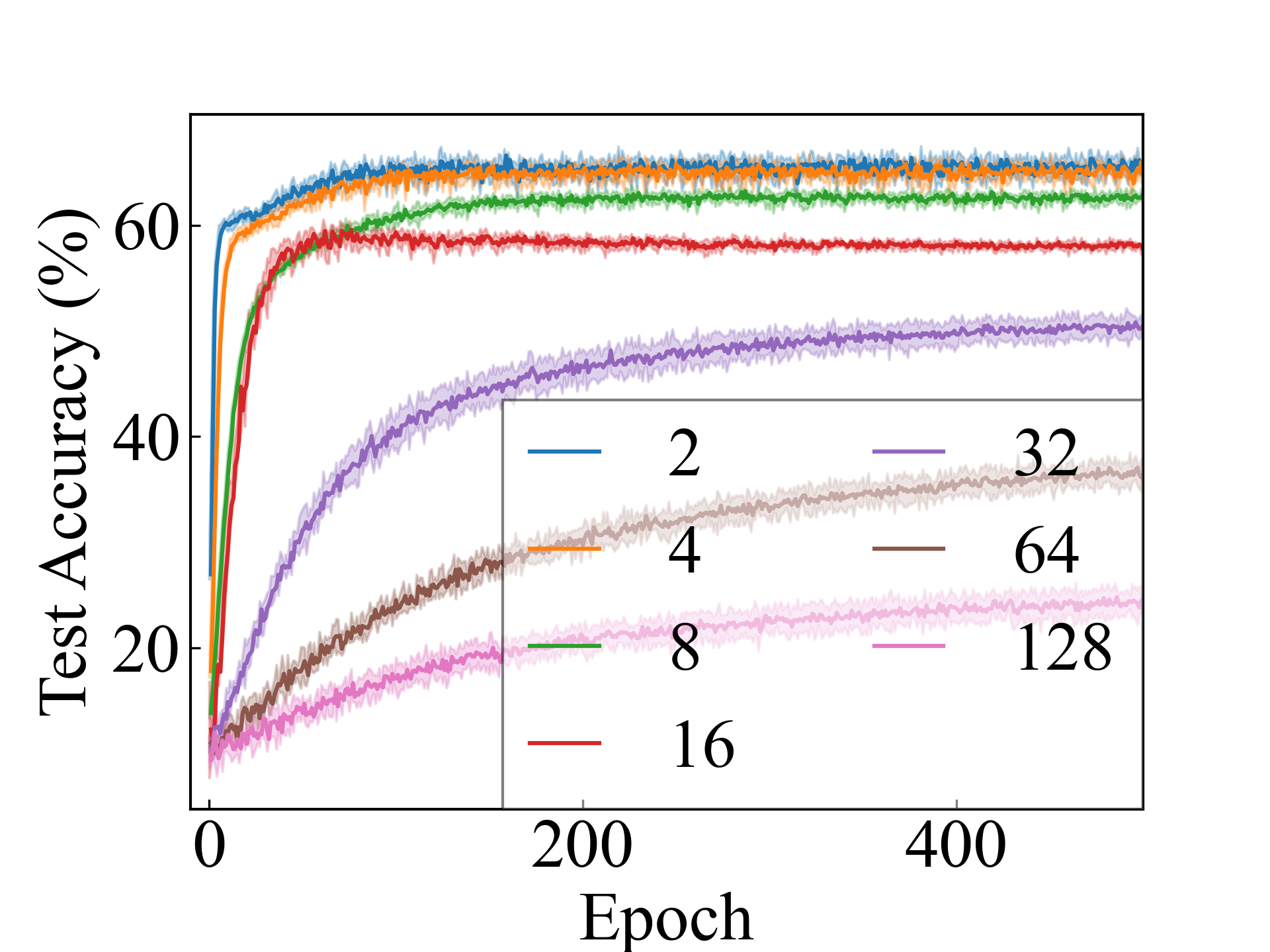
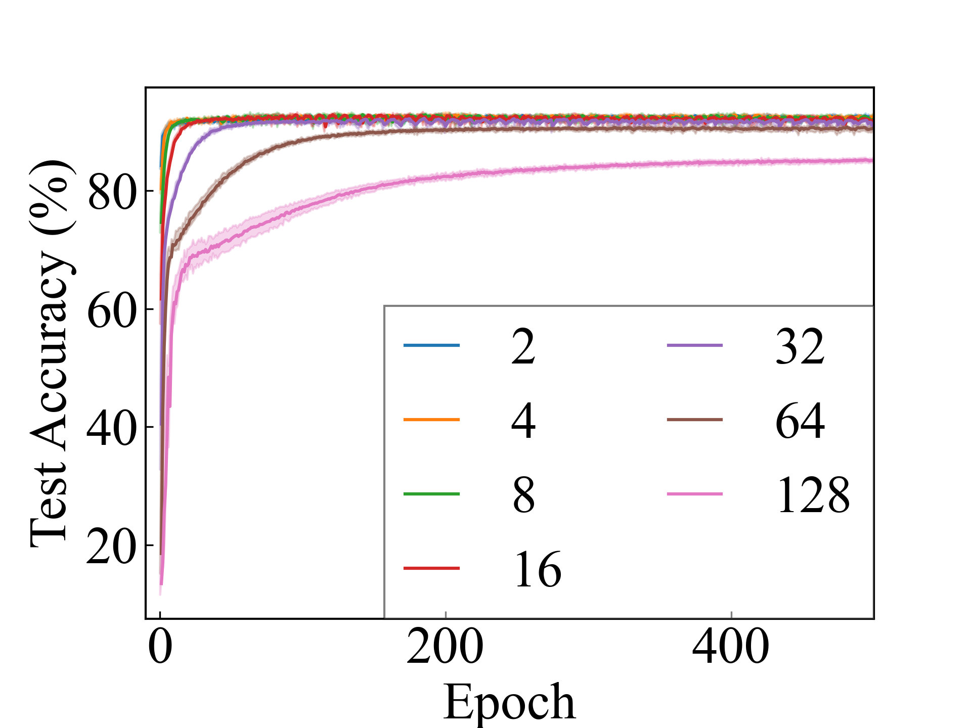
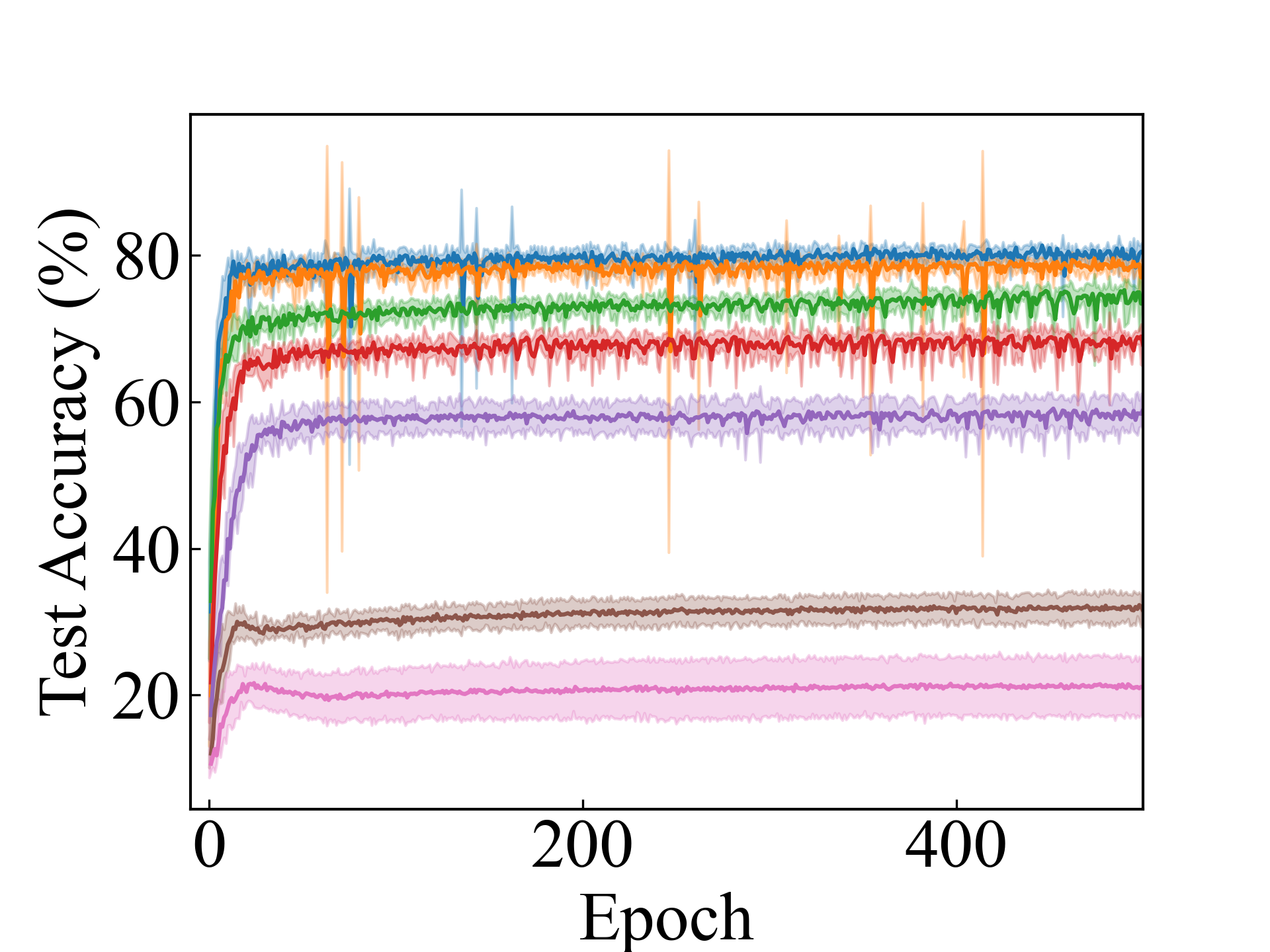
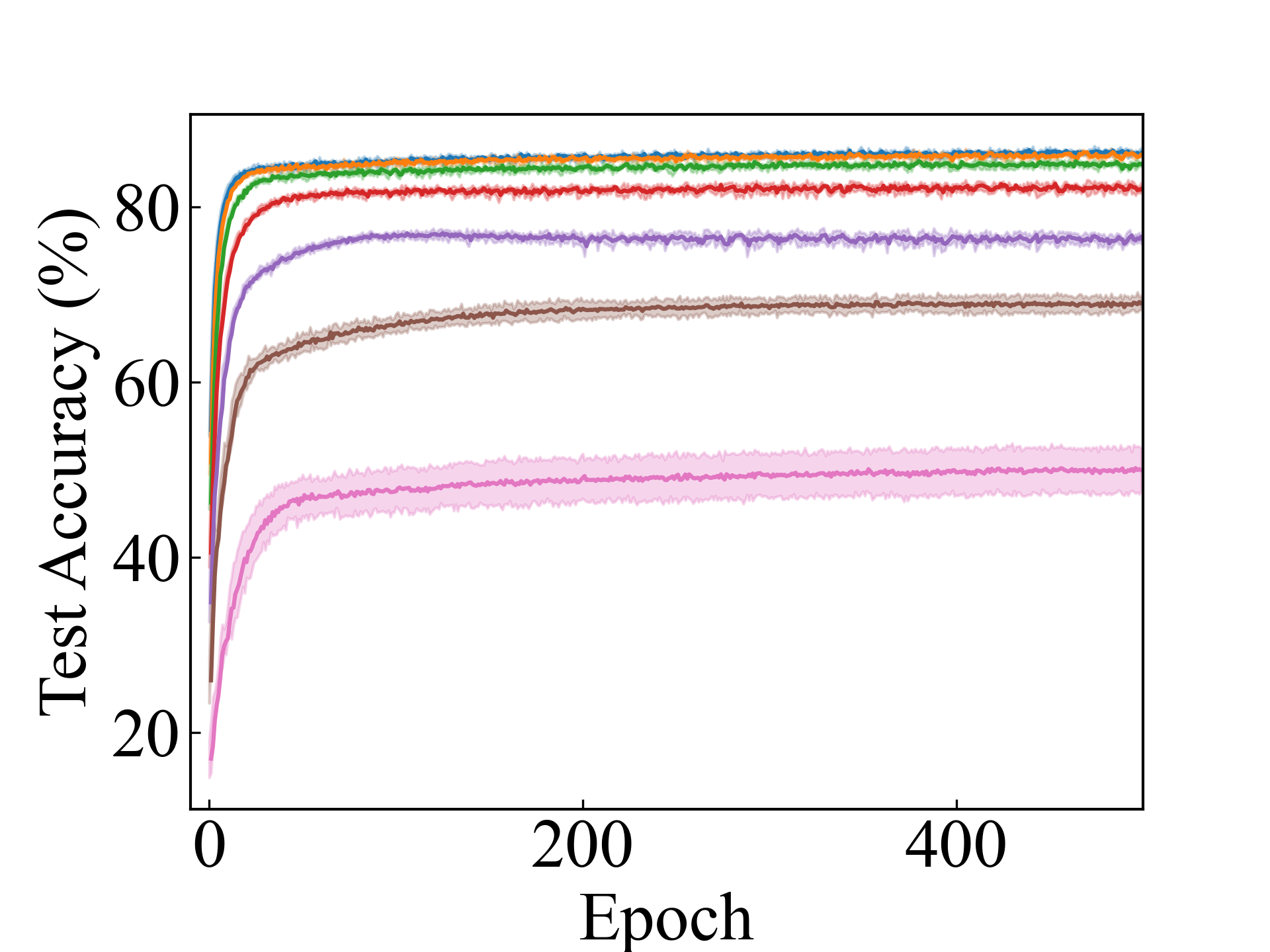
First, we compare the proposed methods with LLPFC and OT, which use the loss per instance. For LLPFC, the proposed methods performed better in many settings in our experiments. As shown in Figure 1, for LLPFC, the training accuracy increased as the loss decreased for simple linear models. However, for complex models, such as deep learning, despite a reduction in the loss, the accuracy decreased—particularly when K was large. A similar phenomenon, in which the accuracy decreases despite decreasing losses when complex models are used, has been observed in various weakly supervised learning studies involving risk estimation, which holds only for the expected values Kiryo et al. (2017); Lu et al. (2020); Chou et al. (2020). Thus, LLPFC may have resulted in biased loss estimations for similar reasons. In contrast, no such trend was observed for the proposed methods. Compared with OT, which generates pseudo-labels through optimal transport, the proposed methods exhibited equal or superior performance, except for the linear model settings. Considering the linear setting results, OT sometimes performed unstably in relatively simple settings such as $K=2$ and 4, as shown in Figure 2, suggesting that the optimal transport labels were unstable during the training.

Subsequently, we compared the proposed methods with DLLP, which takes per-bag losses. While the proposed methods outperformed DLLP, no significant difference was observed among the results of CC, CC_Approx, and DLLP methods in many settings. As discussed in Sec. 5, we can consider DLLP as an approximation method for CC. The results suggest that the same level of performance can be achieved through approximation of the bag-wise loss.

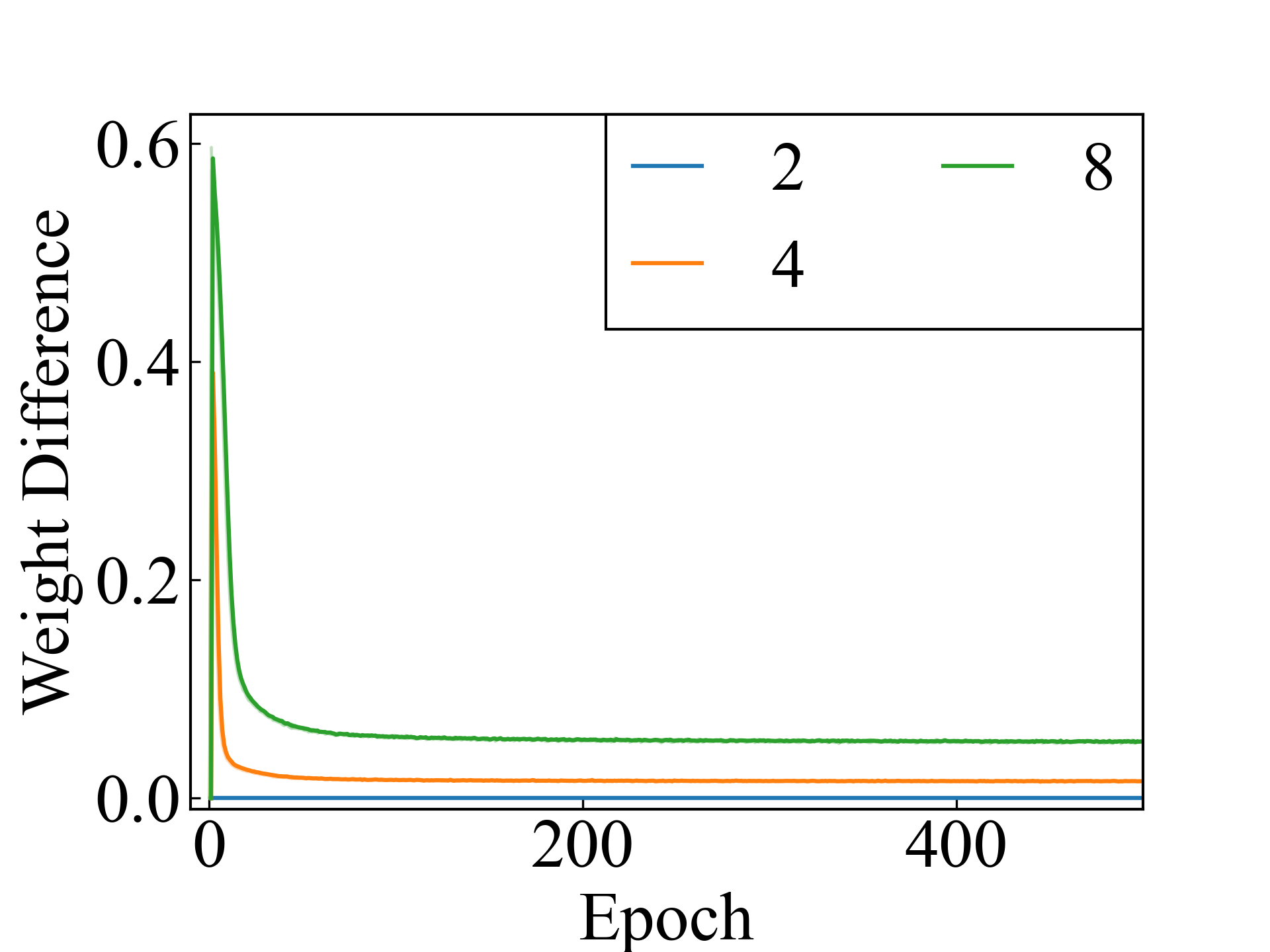
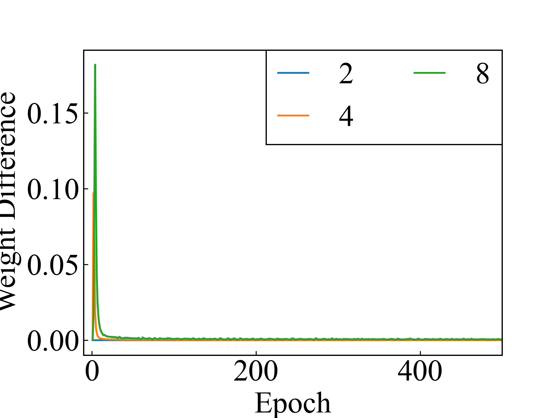
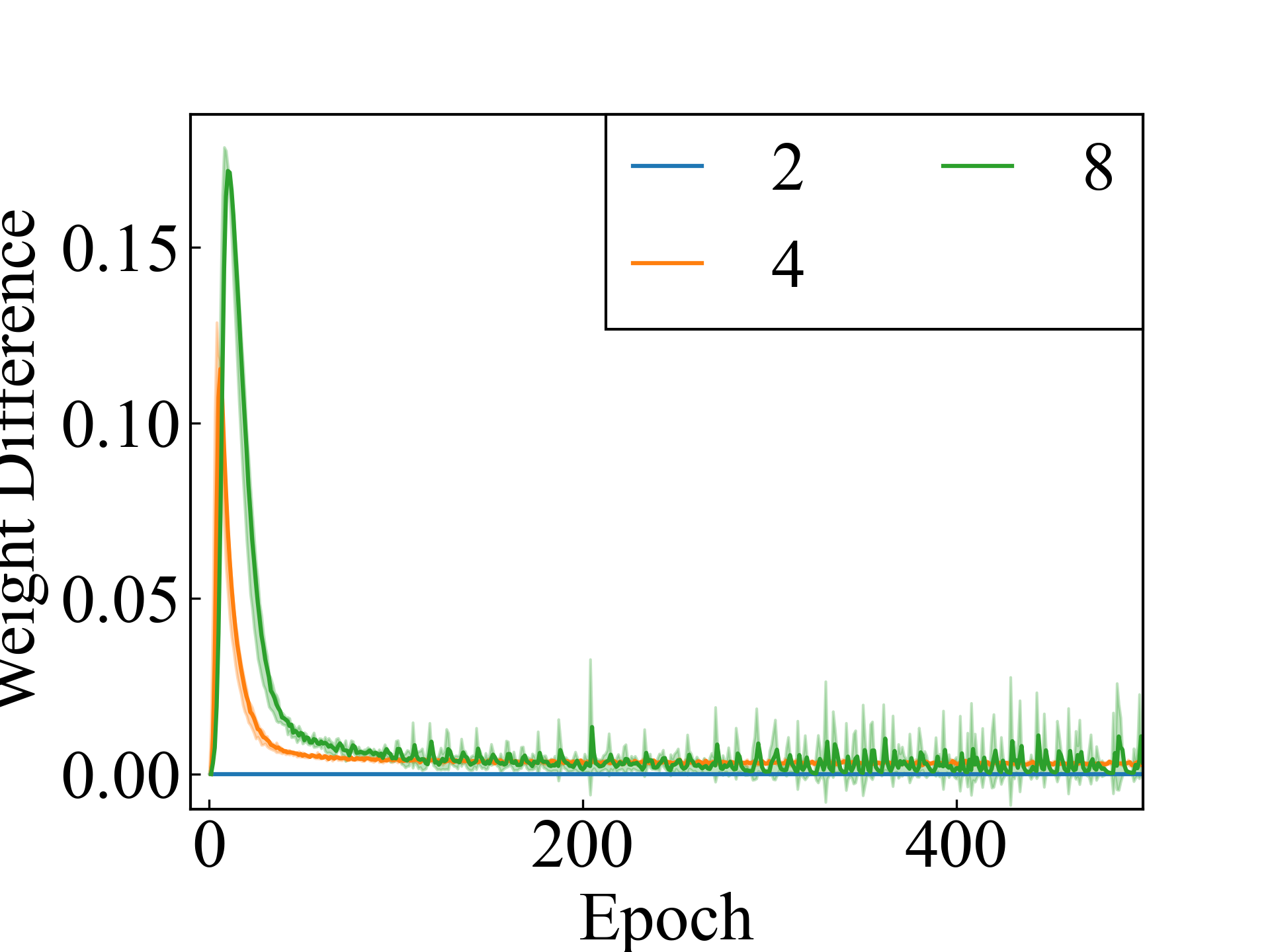
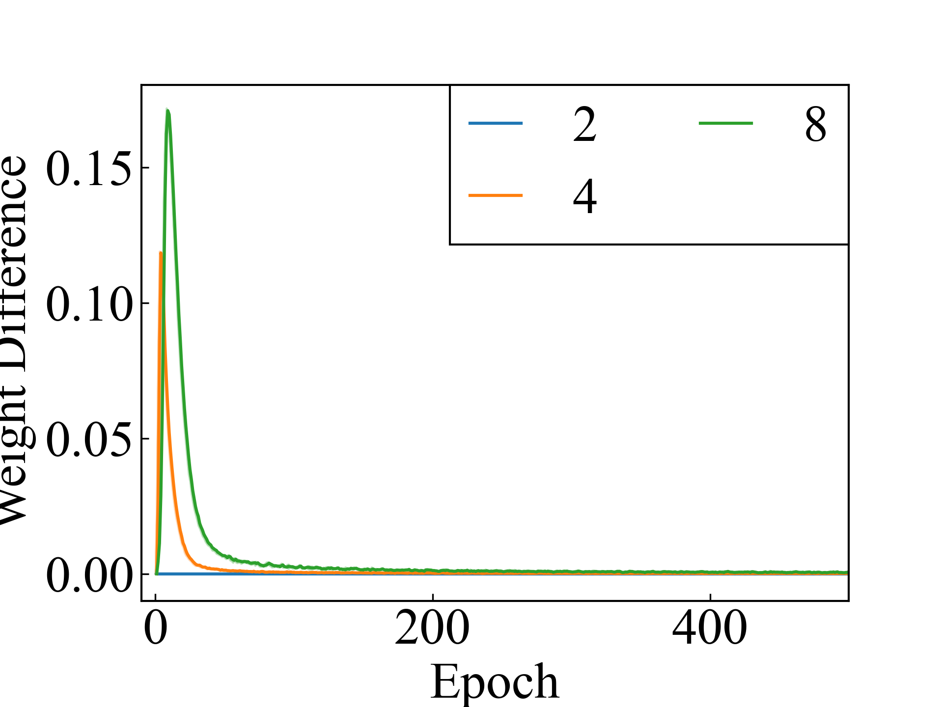
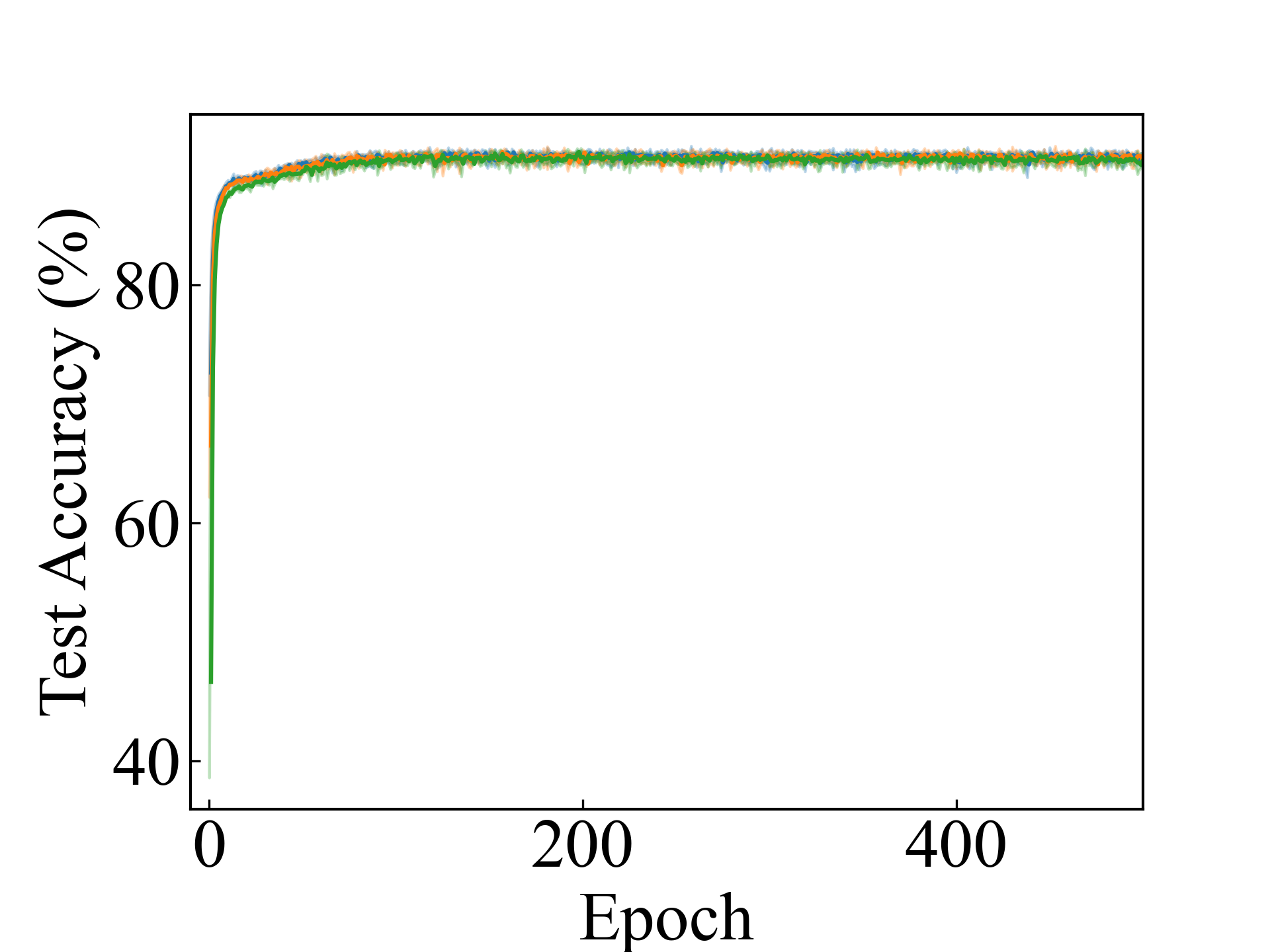
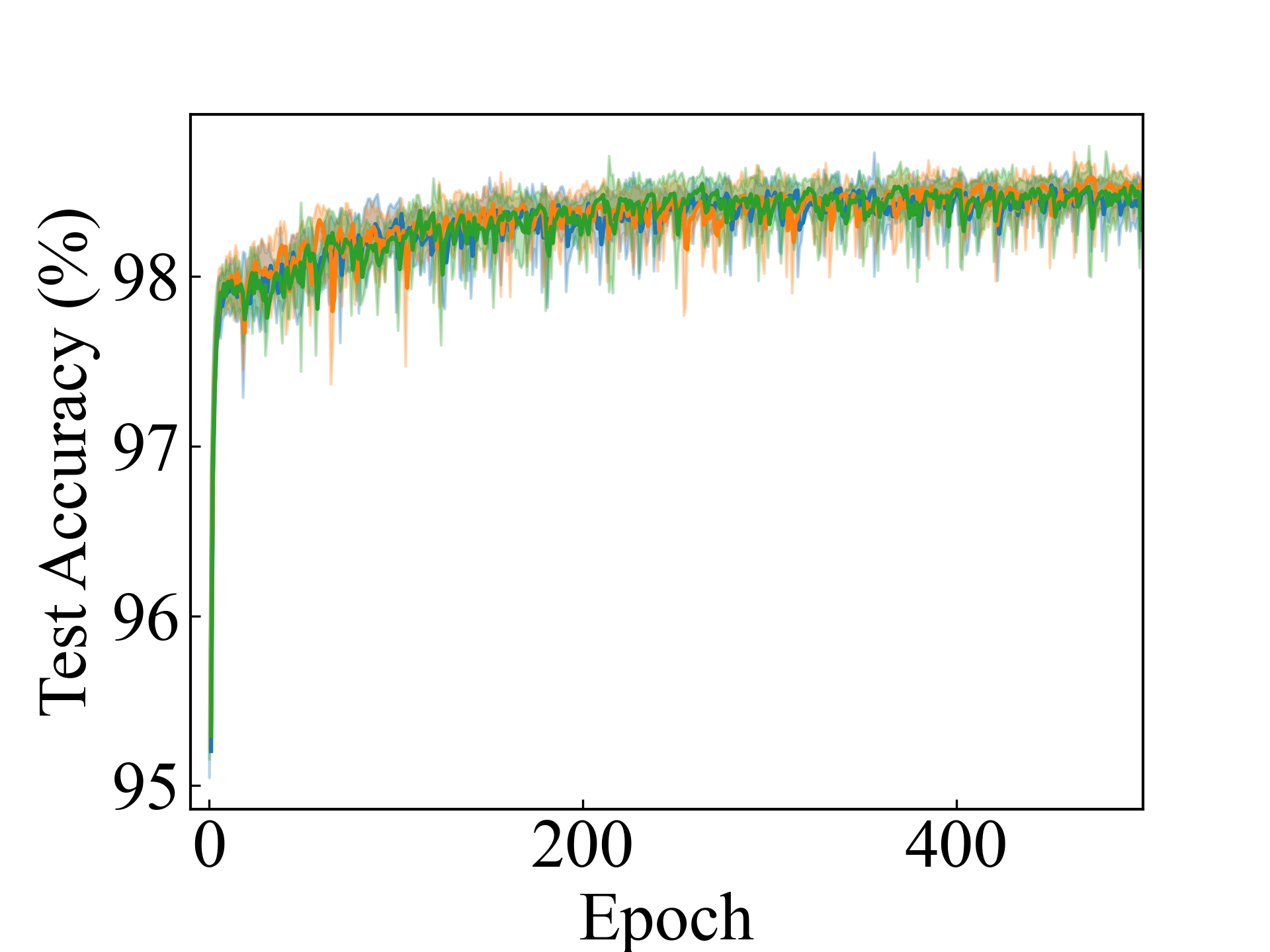
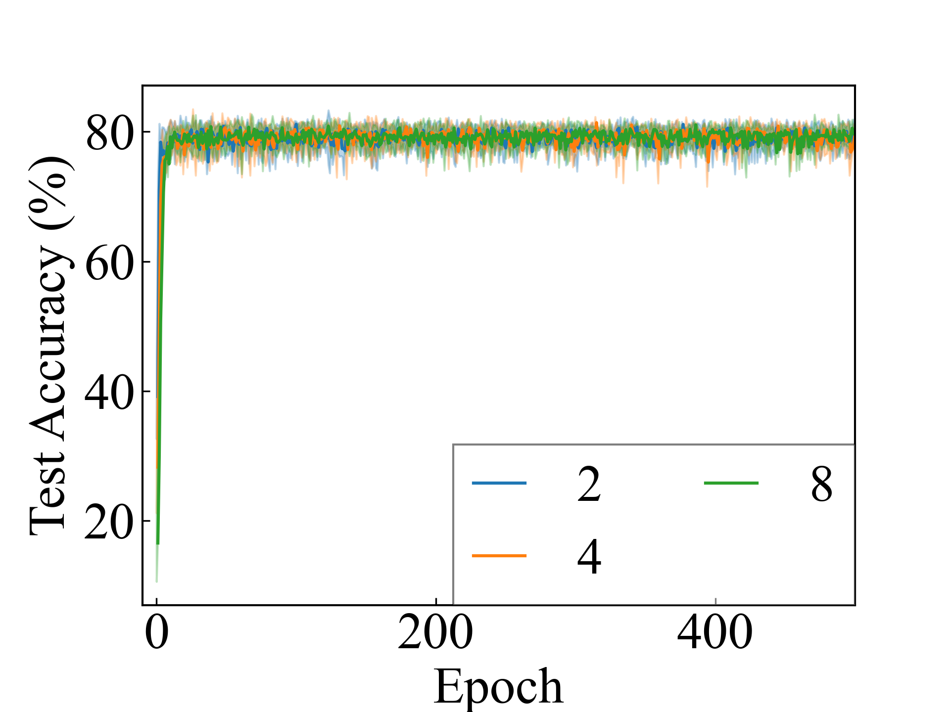
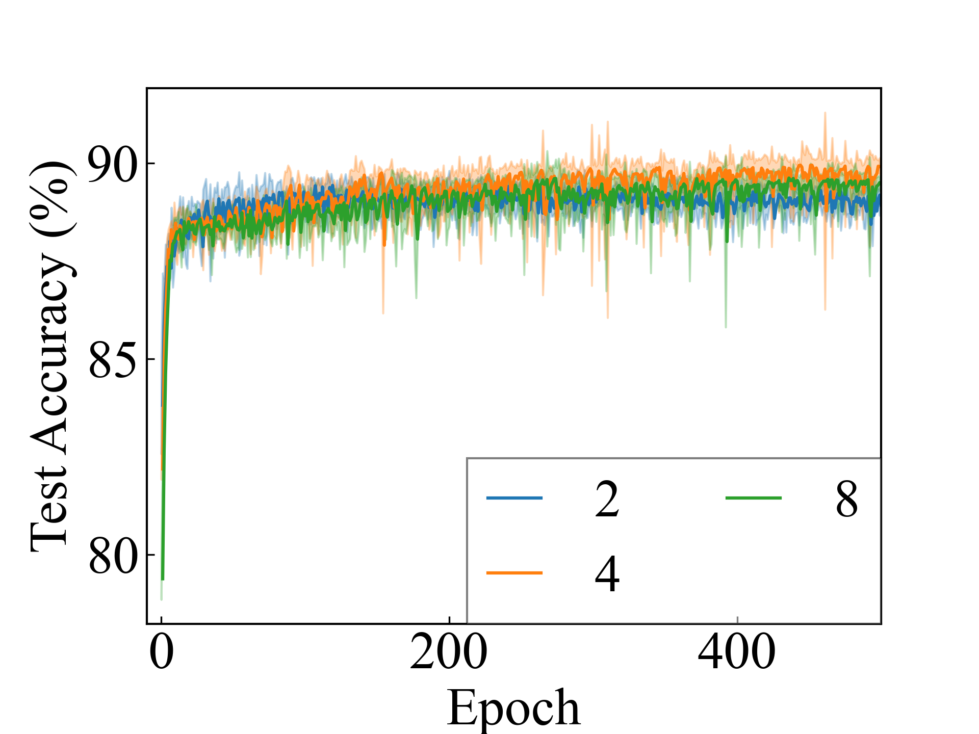
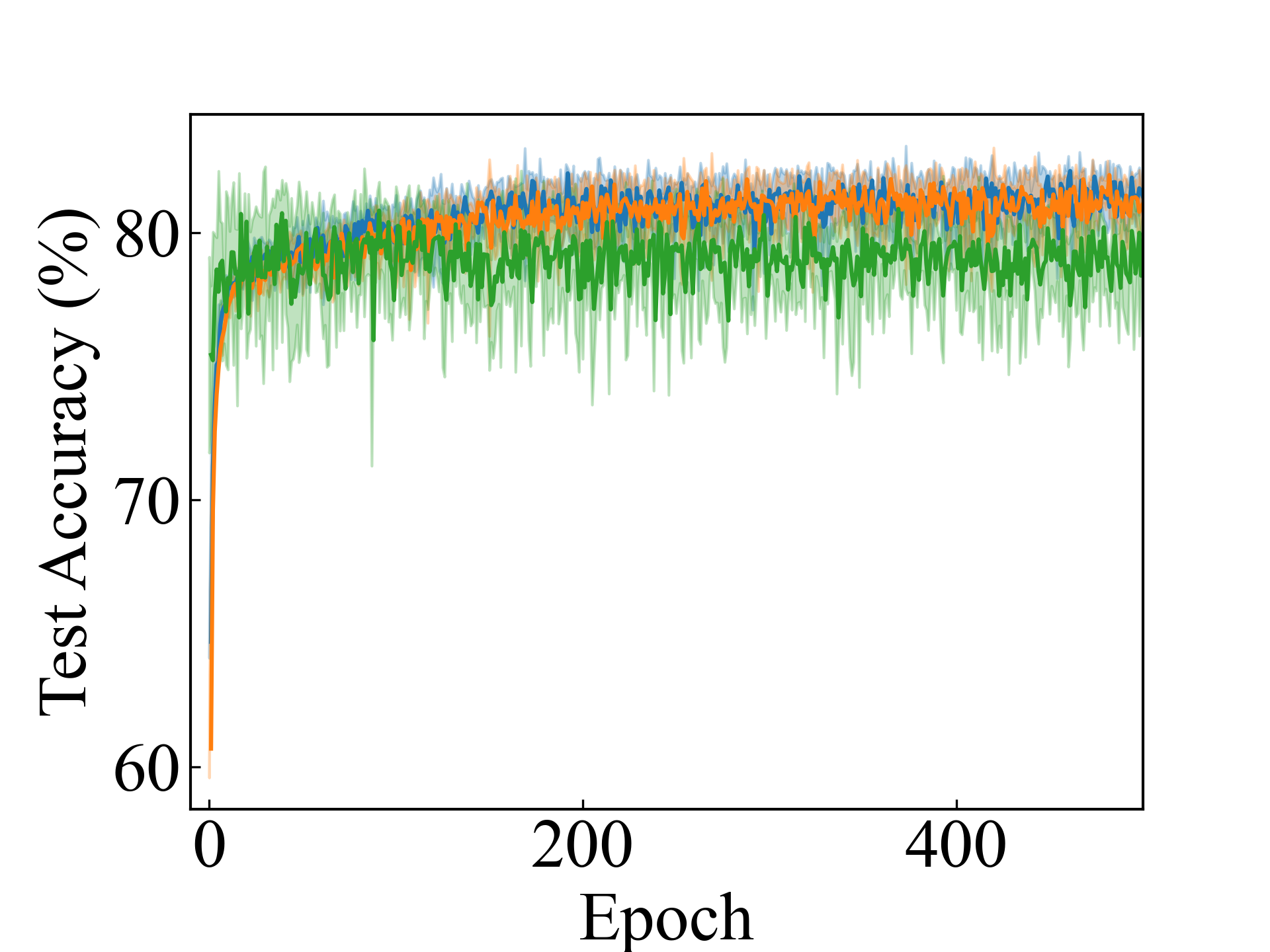
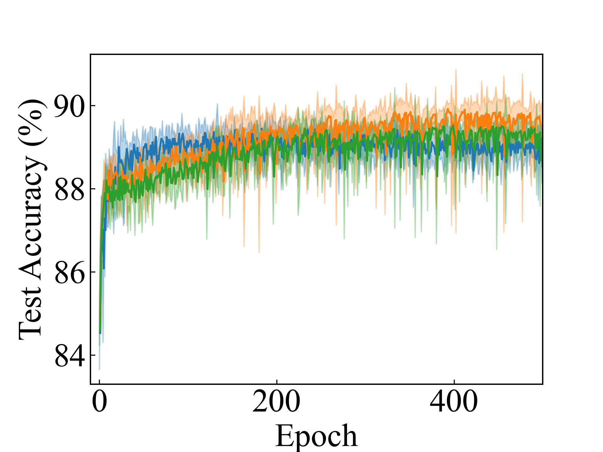
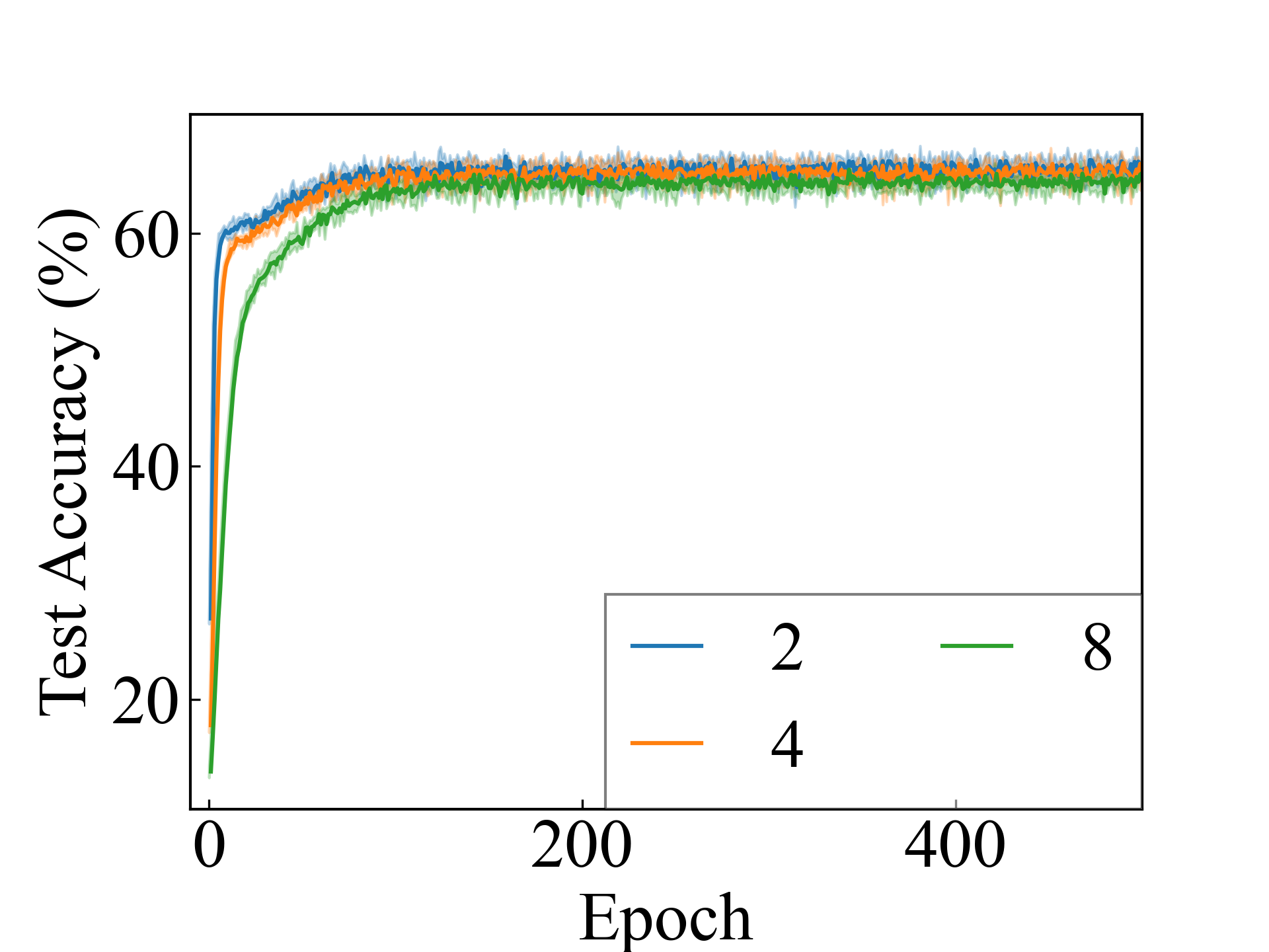
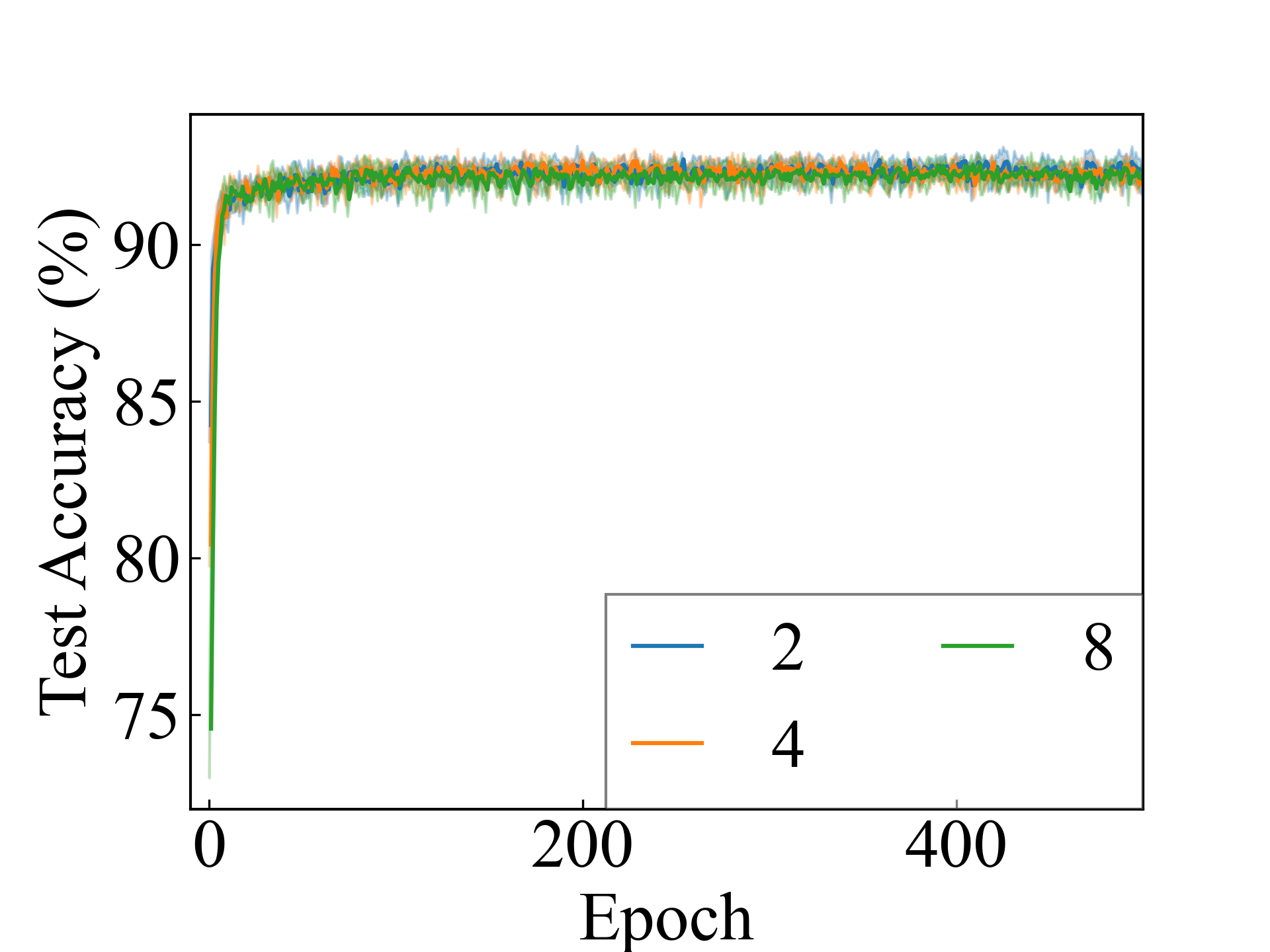
Finally, an approximation method is discussed. The proposed approximation method addresses the memory limitations in experimental setups with $K\geq 16$ , and its performance is comparable to that of non-approximate methods in settings where $K=2,4$ or $8$ . The average difference between the label weights with and without approximation using the RC method is shown in Figure 3. For $K=2$ , the two methods produced the same results, except for the computer error. For $K=4$ and $8$ , the results of the two methods differed, but the difference decreased as the learning converged.

7 Conclusion

We propose learning methods for MCLLP based on statistical learning theory. First, we introduced a method based on per-instance label classification and examined its risk-consistency. We then proposed a method based on the classification of per-bag label proportions and analyzed its classifier-consistency. In addition, we presented a heuristic approximation using a multinomial distribution for the label proportions, which was implicitly used in the previous methods. We discussed partially incorporating this approximation into the proposed methods for reducing the computational complexity. Experimental results confirmed the effectiveness of the proposed methods. Future work will involve integrating the two proposed methods and studying an approximation method with provable guarantees.

Acknowledgements

This work was partially supported by JST AIP Acceleration Research JPMJCR20U3, Moonshot R&D Grant Number JPMJPS2011, CREST Grant Number JPMJCR2015, JSPS KAKENHI Grant Number JP19H01115 and Basic Research Grant (Super AI) of Institute for AI and Beyond of the University of Tokyo.

References

Chapelle et al. [2006] Olivier Chapelle, Bernhard SchÃ¶lkopf, and Alexander Zien. Semi-Supervised Learning. The MIT Press, 2006.
Zhu and Goldberg [2009] Xiaojin Zhu and Andrew Goldberg. 2009.
Sakai et al. [2017] Tomoya Sakai, Marthinus Christoffel Plessis, Gang Niu, and Masashi Sugiyama. Semi-supervised classification based on classification from positive and unlabeled data. In Proceedings of International conference on Machine Learning (ICML), pages 2998–3006, 2017.
Natarajan et al. [2013] Nagarajan Natarajan, Inderjit S Dhillon, Pradeep K Ravikumar, and Ambuj Tewari. Learning with noisy labels. In Advances in Neural Information Processing Systems (NIPS), volume 26, 2013.
Han et al. [2018] Bo Han, Quanming Yao, Xingrui Yu, Gang Niu, Miao Xu, Weihua Hu, Ivor Tsang, and Masashi Sugiyama. Co-teaching: Robust training of deep neural networks with extremely noisy labels. In Advances in Neural Information Processing Systems (NeurIPS), volume 31, 2018.
Amores [2013] Jaume Amores. Multiple instance classification: Review, taxonomy and comparative study. Artificial Intelligence, 201:81–105, 2013.
Ilse et al. [2018] Maximilian Ilse, Jakub Tomczak, and Max Welling. Attention-based deep multiple instance learning. In Proceedings of International Conference on Machine Learning (ICML), pages 2127–2136, 2018.
Feng et al. [2020] Lei Feng, Jiaqi Lv, Bo Han, Miao Xu, Gang Niu, Xin Geng, Bo An, and Masashi Sugiyama. Provably consistent partial-label learning. In Advances in Neural Information Processing Systems (NeurIPS), volume 33, pages 10948–10960, 2020.
Lv et al. [2020] Jiaqi Lv, Miao Xu, Lei Feng, Gang Niu, Xin Geng, and Masashi Sugiyama. Progressive identification of true labels for partial-label learning. In Proceedings of International Conference on Machine Learning (ICML), pages 6500–6510, 2020.
Ishida et al. [2017] Takashi Ishida, Gang Niu, Weihua Hu, and Masashi Sugiyama. Learning from complementary labels. In Advances in Neural Information Processing Systems (NIPS), volume 30, 2017.
du Plessis et al. [2014] Marthinus C du Plessis, Gang Niu, and Masashi Sugiyama. Analysis of learning from positive and unlabeled data. In Advances in Neural Information Processing Systems (NIPS), volume 27, 2014.
Ishida et al. [2018] Takashi Ishida, Gang Niu, and Masashi Sugiyama. Binary classification from positive-confidence data. In Advances in Neural Information Processing Systems (NeurIPS), volume 31, 2018.
Bao et al. [2018] Han Bao, Gang Niu, and Masashi Sugiyama. Classification from pairwise similarity and unlabeled data. In Proceedings of International Conference on Machine Learning (ICML), pages 452–461, 2018.
Shimada et al. [2021] Takuya Shimada, Han Bao, Issei Sato, and Masashi Sugiyama. Classification from pairwise similarities/dissimilarities and unlabeled data via empirical risk minimization. Neural Computation, 33(5):1234–1268, 2021.
Sugiyama et al. [2022] Masashi Sugiyama, Han Bao, Takashi Ishida, Nan Lu, Tomoya Sakai, and Gang Niu. Machine Learning from Weak Supervision. The MIT Press, 2022.
Chen et al. [2014] Tao Chen, Felix X. Yu, Jiawei Chen, Yin Cui, Yan-Ying Chen, and Shih-Fu Chang. Object-based visual sentiment concept analysis and application. In Proceedings of ACM International Conference on Multimedia (ACM MM), page 367â376, 2014.
Lai et al. [2014] Kuan-Ting Lai, Felix X. Yu, Ming-Syan Chen, and Shih-Fu Chang. Video event detection by inferring temporal instance labels. In Proceedings of the IEEE Conference on Computer Vision and Pattern Recognition (CVPR), pages 2251–2258, 2014.
Ding et al. [2017] Yongke Ding, Yuanxiang Li, and Wenxian Yu. Learning from label proportions for sar image classification. EURASIP Journal on Advances in Signal Processing, 2017(1):41, 2017.
Li and Taylor [2015] Fan Li and Graham Taylor. Alter-cnn: An approach to learning from label proportions with application to ice-water classification. In Neural Information Processing Systems Workshops (NIPSW), 2015.
Dery et al. [2017] Lucio Mwinmaarong Dery, Benjamin Nachman, Francesco Rubbo, and Ariel Schwartzman. Weakly supervised classification in high energy physics. Journal of High Energy Physics, 2017(5):1–11, 2017.
Musicant et al. [2007] David R. Musicant, Janara M. Christensen, and Jamie F. Olson. Supervised learning by training on aggregate outputs. In IEEE International Conference on Data Mining (ICDM), pages 252–261, 2007.
Hernández-González et al. [2018] Jerónimo Hernández-González, Iñaki Inza, Lorena Crisol-Ortíz, MarÃa A Guembe, María J I narra, and Jose A Lozano. Fitting the data from embryo implantation prediction: Learning from label proportions. Statistical Methods in Medical Research, 27(4):1056–1066, 2018.
Bortsova et al. [2018] Gerda Bortsova, Florian Dubost, Silas Ørting, Ioannis Katramados, Laurens Hogeweg, Laura Thomsen, Mathilde Wille, and Marleen de Bruijne. Deep learning from label proportions for emphysema quantification. In Proceedings of International Conference on Medical Image Computing and Computer-Assisted Intervention, pages 768–776, 2018.
Poyiadzi et al. [2018] Rafael Poyiadzi, Raul Santos-Rodriguez, and Niall Twomey. Label propagation for learning with label proportions. In IEEE International Workshop on Machine Learning for Signal Processing (MLSP), pages 1–6, 2018.
Zhang et al. [2022] Jianxin Zhang, Yutong Wang, and Clayton Scott. Learning from label proportions by learning with label noise. In Advances in Neural Information Processing Systems (NeurIPS), 2022.
Dulac-Arnold et al. [2019] Gabriel Dulac-Arnold, Neil Zeghidour, Marco Cuturi, Lucas Beyer, and Jean-Philippe Vert. Deep multi-class learning from label proportions. CoRR, 2019.
Liu et al. [2021] Jiabin Liu, Bo Wang, Xin Shen, Zhiquan Qi, and Yingjie Tian. Two-stage training for learning from label proportions. In Proceedings of International Joint Conference on Artificial Intelligence (IJCAI), pages 2737–2743, 2021.
Ardehaly and Culotta [2017] Ehsan Mohammady Ardehaly and Aron Culotta. Co-training for demographic classification using deep learning from label proportions. In IEEE International Conference on Data Mining Workshops (ICDMW), pages 1017–1024, 2017.
Liu et al. [2019] Jiabin Liu, Bo Wang, Zhiquan Qi, YingJie Tian, and Yong Shi. Learning from label proportions with generative adversarial networks. In Advances in Neural Information Processing Systems (NeurIPS), volume 32, 2019.
Tsai and Lin [2020] Kuen-Han Tsai and Hsuan-Tien Lin. Learning from label proportions with consistency regularization. In Proceedings of Asian Conference on Machine Learning (ACML), pages 513–528, 2020.
Yang et al. [2021] Haoran Yang, Wanjing Zhang, and Wai Lam. A two-stage training framework with feature-label matching mechanism for learning from label proportions. In Proceedings of Asian Conference on Machine Learning (ACML), pages 1461–1476, 2021.
BaruÄiÄ and Kybic [2022] Denis BaruÄiÄ and Jan Kybic. Fast learning from label proportions with small bags. In 2022 IEEE International Conference on Image Processing (ICIP), pages 3156–3160, 2022.
Vapnik [1998] Vladimir N. Vapnik. Statistical Learning Theory. 1998.
Wang and Feng [2013] Zilei Wang and Jiashi Feng. Multi-class learning from class proportions. Neurocomputing, 119:273–280, 2013.
Cui et al. [2017] Limeng Cui, Jiawei Zhang, Zhensong Chen, Yong Shi, and Philip S. Yu. Inverse extreme learning machine for learning with label proportions. In IEEE International Conference on Big Data (Big Data), pages 576–585, 2017.
Pérez-Ortiz et al. [2016] M. Pérez-Ortiz, P. A. Gutiérrez, M. Carbonero-Ruz, and C. Hervás-Martínez. Learning from label proportions via an iterative weighting scheme and discriminant analysis. In Proceedings of the Conference of the Spanish Association for Artificial Intelligence, pages 79–88, 2016.
Rüping [2010] Stefan Rüping. Svm classifier estimation from group probabilities. In Proceedings of International Conference on Machine Learning (ICML), pages 911–918, 2010.
Yu et al. [2013] Felix Yu, Dong Liu, Sanjiv Kumar, Jebara Tony, and Shih-Fu Chang. $\propto$ svm for learning with label proportions. In Proceedings of International Conference on Machine Learning (ICML), pages 504–512, 2013.
Qi et al. [2017] Zhiquan Qi, Bo Wang, Fan Meng, and Lingfeng Niu. Learning with label proportions via npsvm. IEEE Transactions on Cybernetics, 47(10):3293–3305, 2017.
Cui et al. [2016] Limeng Cui, Zhensong Chen, Fan Meng, and Yong Shi. Laplacian svm for learning from label proportions. In IEEE International Conference on Data Mining Workshops (ICDMW), pages 847–852, 2016.
Shi et al. [2019] Yong Shi, Limeng Cui, Zhensong Chen, and Zhiquan Qi. Learning from label proportions with pinball loss. International Journal of Machine Learning and Cybernetics, 10(1):187–205, 2019.
Chen et al. [2017] Zhensong Chen, Zhiquan Qi, Bo Wang, Limeng Cui, Fan Meng, and Yong Shi. Learning with label proportions based on nonparallel support vector machines. Knowledge-Based Systems, 119:126–141, 2017.
Wang et al. [2015] Bo Wang, Zhensong Chen, and Zhiquan Qi. Linear twin svm for learning from label proportions. In IEEE/WIC/ACM International Conference on Web Intelligence and Intelligent Agent Technology (WI-IAT), pages 56–59, 2015.
Lu et al. [2019a] Kaili Lu, Xingqiu Zhao, and Bo Wang. A study on mobile customer churn based on learning from soft label proportions. Procedia Computer Science, 162:413–420, 2019a.
Stolpe and Morik [2011] Marco Stolpe and Katharina Morik. Learning from label proportions by optimizing cluster model selection. In Proceedings of European Conference on Machine Learning and Knowledge Discovery in Databases, page 349â364, 2011.
Hernández-González et al. [2013] Jerónimo Hernández-González, Iñaki Inza, and Jose A. Lozano. Learning bayesian network classifiers from label proportions. Pattern Recognition, 46(12):3425–3440, 2013.
Shi et al. [2018] Yong Shi, Jiabin Liu, Zhiquan Qi, and Bo Wang. Learning from label proportions on high-dimensional data. Neural Networks, 103:9–18, 2018.
Quadrianto et al. [2009] Novi Quadrianto, Alex J. Smola, Tibério S. Caetano, and Quoc V. Le. Estimating labels from label proportions. Journal of Machine Learning Research, 10(82):2349–2374, 2009.
Patrini et al. [2014] Giorgio Patrini, Richard Nock, Paul Rivera, and Tiberio Caetano. (almost) no label no cry. In Advances in Neural Information Processing Systems (NIPS), volume 27, 2014.
Lu et al. [2019b] Nan Lu, Gang Niu, Aditya K. Menon, and Masashi Sugiyama. On the minimal supervision for training any binary classifier from only unlabeled data. In Proceedings of International Conference on Learning Representations (ICLR), 2019b.
Scott and Zhang [2020] Clayton Scott and Jianxin Zhang. Learning from label proportions: A mutual contamination framework. In Advances in Neural Information Processing Systems (NeurIPS), volume 33, pages 22256–22267, 2020.
Tang et al. [2022] Yuting Tang, Nan Lu, Tianyi Zhang, and Masashi Sugiyama. Multi-class classification from multiple unlabeled datasets with partial risk regularization. In Proceedings of Asian Conference on Machine Learning (ACML), 2022.
Yu et al. [2015] Felix X. Yu, Krzysztof Choromanski, Sanjiv Kumar, Tony Jebara, and Shih-Fu Chang. On learning from label proportions. CoRR, 2015.
Wu et al. [2022] Zhenguo Wu, Jiaqi Lv, and Masashi Sugiyama. Learning with proper partial labels. Neural Computation, 35:58–81, 2022.
Bartlett and Mendelson [2002] Peter L. Bartlett and Shahar Mendelson. Rademacher and gaussian complexities: Risk bounds and structural results. Journal of Machine Learning Research, 3(11):463–482, 2002.
Golowich et al. [2018] Noah Golowich, Alexander Rakhlin, and Ohad Shamir. Size-independent sample complexity of neural networks. In Proceedings of the Conference On Learning Theory (COLT), volume 75, pages 297–299, 2018.
Yu et al. [2018] Xiyu Yu, Tongliang Liu, Mingming Gong, and Dacheng Tao. Learning with biased complementary labels. In Proceedings of the European Conference on Computer Vision (ECCV), pages 69–85, 2018.
LeCun et al. [1998] Yann LeCun, LÃ©on Bottou, Yoshua Bengio, and Patrick Haffner. Gradient-based learning applied to document recognition. volume 86, pages 2278–2324, 1998.
Xiao et al. [2017] Han Xiao, Kashif Rasul, and Roland Vollgraf. Fashion-mnist: a novel image dataset for benchmarking machine learning algorithms. CoRR, 2017.
Clanuwat et al. [2018] Tarin Clanuwat, Mikel Bober-Irizar, Asanobu Kitamoto, Alex Lamb, Kazuaki Yamamoto, and David Ha. Deep learning for classical japanese literature. CoRR, 2018.
Krizhevsky [2009] Alex Krizhevsky. Learning multiple layers of features from tiny images. 2009.
Samuli Laine [2017] Timo Aila Samuli Laine. Temporal ensembling for semi-supervised learning. In Proceedings of International Conference on Learning Representations (ICLR), 2017.
He et al. [2016] Kaiming He, Xiangyu Zhang, Shaoqing Ren, and Jian Sun. Deep residual learning for image recognition. In Proceedings of the IEEE Conference on Computer Vision and Pattern Recognition (CVPR), pages 770–778, 2016.
Kingma and Ba [2015] Diederik P. Kingma and Jimmy Ba. Adam: A method for stochastic optimization. In Proceedings of International Conference on Learning Representations (ICLR), 2015.
Kiryo et al. [2017] Ryuichi Kiryo, Gang Niu, Marthinus C du Plessis, and Masashi Sugiyama. Positive-unlabeled learning with non-negative risk estimator. In Advances in Neural Information Processing Systems (NIPS), volume 30, 2017.
Lu et al. [2020] Nan Lu, Tianyi Zhang, Gang Niu, and Masashi Sugiyama. Mitigating overfitting in supervised classification from two unlabeled datasets: A consistent risk correction approach. In Proceedings of the International Conference on Artificial Intelligence and Statistics (AISTATS), volume 108, pages 1115–1125, 2020.
Chou et al. [2020] Yu-Ting Chou, Gang Niu, Hsuan-Tien Lin, and Masashi Sugiyama. Unbiased risk estimators can mislead: A case study of learning with complementary labels. In Proceedings of International Conference on Machine Learning (ICML), pages 1929–1938, 2020.
McDiarmid [1989] Colin McDiarmid. On the method of bounded differences. Surveys in combinatorics, 141(1):148–188, 1989.
Maurer [2016] Andreas Maurer. A vector-contraction inequality for rademacher complexities. CoRR, 2016.
Patrini et al. [2017] Giorgio Patrini, Alessandro Rozza, Aditya Krishna Menon, Richard Nock, and Lizhen Qu. Making deep neural networks robust to label noise: A loss correction approach. In Proceedings of the IEEE Conference on Computer Vision and Pattern Recognition (CVPR), pages 1944–1952, 2017.
Flamary et al. [2021] Rémi Flamary, Nicolas Courty, Alexandre Gramfort, Mokhtar Z. Alaya, Aurélie Boisbunon, Stanislas Chambon, Laetitia Chapel, Adrien Corenflos, Kilian Fatras, Nemo Fournier, Léo Gautheron, Nathalie T.H. Gayraud, Hicham Janati, Alain Rakotomamonjy, Ievgen Redko, Antoine Rolet, Antony Schutz, Vivien Seguy, Danica J. Sutherland, Romain Tavenard, Alexander Tong, and Titouan Vayer. Pot: Python optimal transport. Journal of Machine Learning Research, 22(78):1–8, 2021.

Appendix A Proofs

A.1 Proof of Theorem 3.1

First, we derived the estimation error bounds for the risk-consistent method proposed in Sec. 3. We begin by defining the function set $\mathcal{G},\mathcal{G}_{rc}$ as follows:

\displaystyle\mathcal{G}=\{(x,y)\mapsto\ell(f(x),y)|f\in\mathcal{F}\},

\displaystyle\mathcal{G}_{rc}=\{(X,S)\mapsto\frac{1}{K}\sum_{Y\in\mathcal{Y}_{\sigma(S)}^{K}}\frac{P(Y|X)}{P(S|X)}\sum_{k}\ell(f(X^{(k)}),Y^{(k)})|f\in\mathcal{F}\}.

Lemma A.1.

Let $\ell$ denote the loss function and let $M$ denote an upper bound on this function. Then, $\forall\delta>0$ with probability at least $1-\delta$ , we have:

\displaystyle\underset{f\in\mathcal{F}}{\sup}|R_{rc}(f)-\hat{R}_{rc}(f)|\leq 2\mathfrak{R}_{n}(\mathcal{G}_{rc})+M\sqrt{\frac{\log\frac{2}{\delta}}{2n}}.

Proof.

First, consider $\underset{f\in\mathcal{F}}{\sup}R_{rc}(f)-\hat{R}_{rc}(f)$ . Because the loss function satisfies the condition $0\leq\ell(x,y)\leq M$ , replacing one sample $(X,S)$ with another sample $(X^{\prime},S^{\prime})$ does not result in a change in $\underset{f\in\mathcal{F}}{\sup}R_{rc}(f)-\hat{R}_{rc}(f)$ exceeding $\frac{M}{n}$ . Then, using McDiarmid’s inequality McDiarmid [1989], we can assert that $\forall\delta>0$ with a probability of at least $1-\frac{\delta}{2}$ , we have:

\displaystyle\underset{f\in\mathcal{F}}{\sup}R_{rc}(f)-\hat{R}_{rc}(f)\leq\mathbb{E}\left[\underset{f\in\mathcal{F}}{\sup}R_{rc}(f)-\hat{R}_{rc}(f)\right]+M\sqrt{\frac{\log\frac{2}{\delta}}{2n}}.

Furthermore, by utilizing the technique of symmetrization, as described in Vapnik [1998], we demonstrate the following bound:

\displaystyle\mathbb{E}\left[\underset{f\in\mathcal{F}}{\sup}R_{rc}(f)-\hat{R}_{rc}(f)\right]\leq 2\mathfrak{R}_{n}(\mathcal{G}_{rc}).

Additionally, we show that the same bounds hold with a probability of at least $1-\frac{\delta}{2}$ for $\underset{f\in\mathcal{F}}{\sup}\hat{R}_{rc}(f)-R_{rc}(f)$ . ∎

Lemma A.2.

Assuming that the loss function $\ell$ is $\rho$ -Lipschitz, that instances are independently and identically distributed, and that the conditional probability $P(Y|X),P(S|X)$ does not depend on hypothesis $f$ , we can show that the following holds:

\displaystyle\mathfrak{R}_{n}(\mathcal{G}_{rc})\leq\sqrt{2}\rho\sum_{y=1}^{C}\mathfrak{R}_{n}(H_{y}).

Proof.

Let $\phi_{X,S}:\mathbb{R}^{C}\rightarrow\mathbb{R}_{+}$ be defined as

\displaystyle\phi_{X,S}(\bm{z})=\sum_{Y\in\mathcal{Y}_{\sigma(S)}^{K}}\frac{P(Y|X)}{P(S|X)}\ell(\bm{z},Y^{(k)}).

In this case, $\sum_{Y\in\mathcal{Y}_{\sigma(S)}^{K}}\frac{P(Y|X)}{P(S|X)}=1$ , and $\phi_{X,S}$ is a $\rho$ -Lipschitz function. Therefore, the following holds:

	$\displaystyle\mathfrak{R}_{n}(\mathcal{G}_{rc})$	$\displaystyle=\mathbb{E}\left[\underset{g\in\mathcal{G}_{rc}}{\sup}\sum_{i}^{n}\sigma_{i}g(X_{i},S_{i})\right]$
		$\displaystyle=\mathbb{E}\left[\underset{f\in\mathcal{F}}{\sup}\sum_{i}^{n}\sigma_{i}\frac{1}{K}\sum_{k}\sum_{Y\in\mathcal{Y}_{\sigma(S)}^{K}}\frac{P(Y\|X)}{P(S\|X)}\ell(f(X^{(k)}),Y^{(k)})\right]$
		$\displaystyle=\mathbb{E}\left[\underset{f\in\mathcal{F}}{\sup}\sum_{i}^{n}\sigma_{i}\frac{1}{K}\sum_{k}\phi_{X,S}(f(X^{(k)}))\right]$
		$\displaystyle=\frac{1}{K}\sum_{k}\mathbb{E}\left[\underset{f\in\mathcal{F}}{\sup}\sum_{i}^{n}\sigma_{i}\phi_{X,S}(f(X^{(k)}))\right]$
		$\displaystyle\leq\sqrt{2}\rho\mathbb{E}\left[\underset{f\in\mathcal{F}}{\sup}\sum_{i}^{n}\sum_{c}\sigma_{ic}f(X^{(1)})\right]$
		$\displaystyle=\sqrt{2}\rho\sum_{c}\mathfrak{R}_{n}(\mathcal{H}_{c}).$

When deriving this result, the Rademacher vector contraction inequality Maurer [2016] was employed for the second line from the end. ∎

From Lemmas A.1 and A.2, we obtain the following estimated error bounds:

	$\displaystyle R_{rc}(\hat{f})-R_{rc}(f^{*})$	$\displaystyle\leq R_{rc}(\hat{f})-\hat{R}_{rc}(\hat{f})+\hat{R}_{rc}(\hat{f})-R_{rc}(f^{*})$
		$\displaystyle\leq R_{rc}(\hat{f})-\hat{R}_{rc}(\hat{f})+R_{rc}(\hat{f})-R_{rc}(f^{*})$
		$\displaystyle\leq 2\underset{f\in F}{\sup}\|\hat{R}_{rc}(f)-R_{rc}(f)\|$
		$\displaystyle\leq 4\mathfrak{R}_{n}(\mathcal{G}_{rc})+2M\sqrt{\frac{\log\frac{2}{\delta}}{2n}}$
		$\displaystyle\leq 4\sqrt{2}\rho\sum_{y=1}^{C}\mathfrak{R}_{n}(\mathcal{H}_{y})+2M\sqrt{\frac{\log\frac{2}{\delta}}{2n}}.$

$\Box$

A.2 Proof of Theorem 4.2

Proof.

First, we set the quantity $\bm{Q}\in\mathbb{R}^{{}_{K}H_{C}\times C}$ as follows:

\displaystyle\bm{Q}_{ij}(X\backslash X^{(k)})=\begin{cases}P(T_{i}\backslash j|X\backslash X^{(k)})&\text{if~{}}j\in T_{i},\\ 0&\text{otherwise}.\end{cases}

Let $\bm{v}_{S}=\left[P(S=T_{1}|X),\cdots,P(S=T_{{}_{K}H_{C}}|X)\right]^{\mathsf{T}}\in\mathbb{R}^{{}_{K}H_{C}}$ and $\bm{v}_{y}=\left[P(y=1|X^{(k)}),\cdots,P(y=C|X^{(k)})\right]^{\mathsf{T}}\in\mathbb{R}^{C}$ . Then, $\forall k\in\{1,\cdots,C\}$ , $\bm{v}_{S}$ and $\bm{v}_{y}$ have the following relationship:

\displaystyle\bm{v}_{S}=\bm{Q}\bm{v}_{y}.

Furthermore, as a result of Lemma 4.1 Yu et al. [2018], it can be shown that the optimal classifier $q^{*}$ learned with the cross-entropy loss and mean squared error loss satisfies $q_{i}^{*}=P(S=T_{i}|X)$ , and $q^{*}(X)=\bm{v}_{S}$ holds. Let $e^{*}(X^{(k)})$ denote the softmax output of the classifier that minimizes the $R_{cc}$ as specified in Eq. 12. Then $q^{*}(X)=\bm{Q}e^{*}(X^{(k)})$ holds. Additionally, because $\bm{Q}$ is full column rank, $e^{*}_{i}(X^{(k)})=P(y=i|X^{(k)})$ holds. ∎

A.3 Proof of Theorem 4.3

We derive the estimation error bounds for the classifier-consistent method proposed in Sec. 4 by following the same procedure used in Sec. A.3. We begin by defining the function set $\mathcal{G}_{cc}$ as follows:

\displaystyle\mathcal{G}_{cc}=\{(X,S)\mapsto\frac{1}{K}\sum_{k}\mathcal{L}(q(s(X^{(k)},k)),S)|f\in\mathcal{F}\}.

Lemma A.3.

Let $\mathcal{L}$ denote the loss function and let $M$ denote an upper bound on this function. Then, $\forall\delta>0$ with a probability of at least $1-\delta$ , we have

\displaystyle\underset{f\in\mathcal{F}}{\sup}|R_{cc}(f)-\hat{R}_{cc}(f)|\leq 2\mathfrak{R}_{n}(\mathcal{G}_{cc})+M\sqrt{\frac{\log\frac{2}{\delta}}{2n}}.

Proof.

We first consider $\underset{f\in\mathcal{F}}{\sup}R_{cc}(f)-\hat{R}_{cc}(f)$ . As the loss function satisfies the condition $0\leq\mathcal{L}(x,y)\leq M$ , replacing one sample $(X,S)$ with another sample $(X^{\prime},S^{\prime})$ does not result in a change in $\underset{f\in\mathcal{F}}{\sup}R_{cc}(f)-\hat{R}_{cc}(f)$ exceeding $\frac{M}{n}$ . Then, using McDiarmid’s inequality McDiarmid [1989], we can assert that $\forall\delta>0$ with a probability of at least $1-\frac{\delta}{2}$ , we have:

\displaystyle\underset{f\in\mathcal{F}}{\sup}R_{cc}(f)-\hat{R}_{cc}(f)\leq\mathbb{E}\left[\underset{f\in\mathcal{F}}{\sup}R_{cc}(f)-\hat{R}_{cc}(f)\right]+M\sqrt{\frac{\log\frac{2}{\delta}}{2n}}.

Furthermore, by utilizing the technique of symmetrization, as described in Vapnik [1998], we demonstrate the following bound:

\displaystyle\mathbb{E}\left[\underset{f\in\mathcal{F}}{\sup}R_{cc}(f)-\hat{R}_{cc}(f)\right]\leq 2\mathfrak{R}_{n}(\mathcal{G}_{cc}).

Additionally, we show that the same bounds hold with a probability of at least $1-\frac{\delta}{2}$ for $\underset{f\in\mathcal{F}}{\sup}\hat{R}_{cc}(f)-R_{cc}(f)$ . ∎

Lemma A.4.

Assuming that the loss function $\mathcal{L}$ is $\rho$ -Lipschitz, that the instances are independently and identically distributed, and that $\bm{Q}$ does not depend on the hypothesis $f$ , it can be shown that the following holds:

\displaystyle\mathfrak{R}_{n}(\mathcal{G}_{cc})\leq\sqrt{2}\rho\sum_{y=1}^{C}\mathfrak{R}_{n}(H_{y}).

Proof.

Let $\phi_{X,S}:\mathbb{R}^{C}\rightarrow\mathbb{R}_{+}$ be defined as

\displaystyle\phi_{X,T_{j}}(\bm{z})=\mathcal{L}(\bm{Q}[j]^{\mathsf{T}}\bm{z},T_{j}).

In this case, $\bm{Q}$ has the property that the sum of the elements in each row is less than 1, and $\phi_{X,S}$ is a $\rho$ -Lipschitz function. Therefore, the following holds:

	$\displaystyle\mathfrak{R}_{n}(\mathcal{G}_{cc})$	$\displaystyle=\mathbb{E}\left[\underset{g\in\mathcal{G}_{cc}}{\sup}\sum_{i}^{n}\sigma_{i}g(X_{i},S_{i})\right]$
		$\displaystyle=\mathbb{E}\left[\underset{f\in\mathcal{F}}{\sup}\sum_{i}^{n}\sigma_{i}\frac{1}{K}\sum_{k}\mathcal{L}(q(s(X^{(k)},k)),S)\right]$
		$\displaystyle=\mathbb{E}\left[\underset{f\in\mathcal{F}}{\sup}\sum_{i}^{n}\sigma_{i}\frac{1}{K}\sum_{k}\phi_{X,S}(f(s(X^{(k)},k)))\right]$
		$\displaystyle=\frac{1}{K}\sum_{k}\mathbb{E}\left[\underset{f\in\mathcal{F}}{\sup}\sum_{i}^{n}\sigma_{i}\phi_{X,S}(f(s(X^{(k)},k)))\right]$
		$\displaystyle\leq\sqrt{2}\rho\mathbb{E}\left[\underset{f\in\mathcal{F}}{\sup}\sum_{i}^{n}\sum_{c}\sigma_{ic}f(X^{(1)})\right]$
		$\displaystyle=\sqrt{2}\rho\sum_{c}\mathfrak{R}_{n}(\mathcal{H}_{c}).$

We use the Rademacher vector contraction inequality Maurer [2016] in the second line from the end. ∎

From Lemmas A.3 and A.4, we obtain the following estimated error bounds:

	$\displaystyle R_{cc}(\hat{f})-R_{cc}(f^{*})$	$\displaystyle\leq R_{cc}(\hat{f})-\hat{R}_{cc}(\hat{f})+\hat{R}_{cc}(\hat{f})-R_{cc}(f^{*})$
		$\displaystyle\leq R_{cc}(\hat{f})-\hat{R}_{cc}(\hat{f})+R_{cc}(\hat{f})-R_{cc}(f^{*})$
		$\displaystyle\leq 2\underset{f\in F}{\sup}\|\hat{R}_{cc}(f)-R_{cc}(f)\|$
		$\displaystyle\leq 4\mathfrak{R}_{n}(\mathcal{G}_{cc})+2M\sqrt{\frac{\log\frac{2}{\delta}}{2n}}$
		$\displaystyle\leq 4\sqrt{2}\rho\sum_{y=1}^{C}\mathfrak{R}_{n}(\mathcal{H}_{y})+2M\sqrt{\frac{\log\frac{2}{\delta}}{2n}}.$

$\Box$

Appendix B Experimental Settings

B.1 Datasets

In this study, we conducted experiments with four commonly used datasets.

•

MNIST LeCun et al. [1998]: 10-class datasets of handwritten digits. Each image is grayscale and has a size of 28 $\times$ 28.
•

Fashion-MNIST Xiao et al. [2017]: 10-class datasets of fashion items. Each image is grayscale and has a size of 28 $\times$ 28.
•

Kuzushiji-MNIST Clanuwat et al. [2018]: 10-class datasets of Japanese handwritten kuzushiji, i.e., cursive writing style letters. Each image is grayscale and has a size of 28 $\times$ 28.
•

CIFAR-10 Krizhevsky [2009]: 10-class datasets of vehicles and animals. Each image has an RGB channel and has a size of 32 $\times$ 32 pixels.

B.2 Models

We used linear and MLP models for MNIST, Fashion-MNIST, Kuzushiji-MNIST, and ConvNet and ResNet models for the CIFAR-10 dataset. The linear model refers to a $d$ – $10$ linear function, where $d$ represents the input size. The MLP was a 5-layer perceptron $d$ – $300$ – $300$ – $300$ – $300$ – $10$ with ReLU activation. Each dense layer was subjected to batch normalization. The ConvNet architecture is described in Table 5.

B.3 comparison methods

We performed comparative experiments with the LLPFC Zhang et al. [2022], OT Liu et al. [2021], and DLLP Ardehaly and Culotta [2017] methods. In this section, we describe the experimental setup—particularly for LLPFC and OT, which had specific parameters.

LLPFC Zhang et al. [2022] LLPFC is a method that performs LLP via forward correction of label noise Patrini et al. [2017]. We implemented the LLPFC-uniform algorithm according to the implementation provided on Github ²²2https://github.com/Z-Jianxin/LLPFC. As a specific parameter, the groups were updated every 20 epochs following the reference implementation.

OT Liu et al. [2021] OT is a method that takes into account the classification loss per instance using pseudo-labels created by optimal transport. Liu et al. [2021] proposed using per-instance losses with pseudo-labels generated by optimal transport after utilizing per-bag losses. However, in our study, we implemented OT to update the weights during learning in the same way as the $R_{rc}$ method to facilitate a direct comparison with our methods. We implemented optimal transport using the POT Flamary et al. [2021] Sinkhorn algorithm. The number of optimization was set to 75, and the entropy constraint factor $\epsilon$ was set as 1, following the guidelines of Dulac-Arnold et al. [2019].

Input 3 $\times$ 32 $\times$ 32 image
3 $\times$ 3 conv. 128 followed by LeakyReLU $\times$ 3
max-pooling, dropout with $p=0.25$
3 $\times$ 3 conv. 256 followed by LeakyReLU $\times$ 3
max-pooling, dropout with $p=0.25$
3 $\times$ 3 conv. 512 followed by LeakyReLU $\times$ 3
global mean pooling, Dense 10

Table 5: ConvNet model for CIFAR-10.

Appendix C Experimental Results

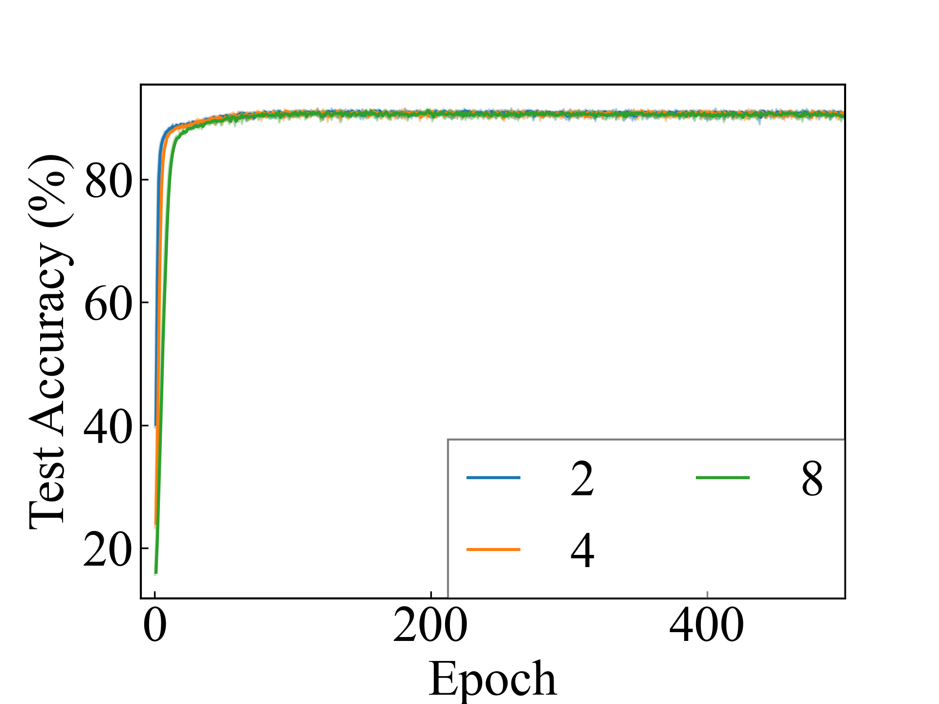
We present the test accuracy for the linear models in Table 1 and the test accuracy curve for the proposed methods in Figure 5.

	$\displaystyle P(S\|X)$	$\displaystyle=\sum_{Y\in\mathcal{Y}^{K}}P(Y,S\|X)\overset{(\ref{eq:PYSX})}{=}\sum_{Y\in\mathcal{Y}_{\sigma(S)}^{K}}P(Y\|X)$
		$\displaystyle\overset{(\ref{eq:PYX})}{=}\sum_{y\in\mathit{set}(S)}P(y\|X^{(k)})P(S\backslash y\|X\backslash X^{(k)}).$		(9)

Learning from Label Proportions with Instance-wise Consistency

Abstract

1 Introduction

2 Formulations and Related Studies

2.1 Standard Multiclass Classification

2.2 LLP

2.3 PLL

3 Per-Instance Method

3.1 Risk Estimation

3.2 Risk-Consistency & Estimation Error Bound

Theorem 3.1.

3.3 Learning Method

4 Per-Bag Method

4.1 Risk Estimation

4.2 Classifier-Consistency & Estimation Error Bound

Lemma 4.1.

Theorem 4.2.

Theorem 4.3.

4.3 Learning Method

5 Approximation Method

5.1 DLLP as likelihood maximization

5.2 Approximation with Mean Operation

6 Experiments

7 Conclusion

Acknowledgements

References

Appendix A Proofs

A.1 Proof of Theorem 3.1

Lemma A.1.

Proof.

Lemma A.2.

Proof.

A.2 Proof of Theorem 4.2

Proof.

A.3 Proof of Theorem 4.3

Lemma A.3.

Proof.

Lemma A.4.

Proof.

Appendix B Experimental Settings

B.1 Datasets

B.2 Models

B.3 comparison methods

Appendix C Experimental Results

Learning from Label Proportions
with Instance-wise Consistency