Learning Implicit Generative Models Using
Differentiable Graph Tests
Abstract
Recently, there has been a growing interest in the problem of learning rich implicit models — those from which we can sample, but can not evaluate their density. These models apply some parametric function, such as a deep network, to a base measure, and are learned end-to-end using stochastic optimization. One strategy of devising a loss function is through the statistics of two sample tests — if we can fool a statistical test, the learned distribution should be a good model of the true data. However, not all tests can easily fit into this framework, as they might not be differentiable with respect to the data points, and hence with respect to the parameters of the implicit model. Motivated by this problem, in this paper we show how two such classical tests, the Friedman-Rafsky and -nearest neighbour tests, can be effectively smoothed using ideas from undirected graphical models – the matrix tree theorem and cardinality potentials. Moreover, as we show experimentally, smoothing can significantly increase the power of the test, which might of of independent interest. Finally, we apply our method to learn implicit models.
1 Introduction
The main motivation for our work is that of learning implicit models, i.e., those from which we can easily sample, but can not evaluate their density. Formally, we can generate a sample from an implicit distribution by first drawing from some known and fixed distribution , typically Gaussian or uniform, and then passing it through some differentiable function parametrized by some vector to generate . The goal is then to optimize the parameters of the mapping so that is as close as possible to some target distribution , which we can access only via iid samples. The approach that we undertake in this paper is that of defeating statistical two-sample tests. These tests operate in the following setting — given two sets of iid samples, from , and from , we have to distinguish between the following hypotheses
The tests that we consider start by defining a function that should result in a low value if the two samples come from different distributions. Then, the hypothesis is rejected at significance level if is lower than some threshold , which is computed using a permutation test, as explained in Section 2. Going back the original problem, one intuitive approach would be to maximize the expected statistic using stochastic optimization over the parameters of the mapping . However, this requires the availability of the derivatives , which is unfortunately not always possible. For example, the Friedman-Rafsky (FR) and -nearest neighbours (-NN) tests, which have very desirable statistical properties (including consistency and convergence of their statistics to -divergences), can not be cast in the above framework as they use the output of a combinatorial optimization problem. Our main contribution is the development of differentiable versions of these tests that remedy the above problem by smoothing their statistics. We moreover show, similarly to these classical tests, that our tests are asymptotically normal under certain conditions, and derive the corresponding -statistic, which can be evaluated with minimal additional complexity. Our smoothed tests can have more power over their classical variants, as we showcase with numerical experiments. Finally, we experimentally learn implicit models in Section 5.
Related work.
The problem of two-sample testing for distributional equality has received significant interest in statistics. For example, the celebrated Kolmogorov-Smirnov test compares two one dimensional distributions by taking the maximal difference of the empirical CDFs. Another one-dimensional test is the runs test of Wald and Wolfowitz [1], which has been extended to the multivariate case by Friedman and Rafsky [2] (FR). It is exactly this test, together with -NN test originally suggested in [3] that we analyze. These tests have been analyzed in more detail by Henze and Penrose [4], and Henze [5], Schilling [6] respectively. Their asymptotic efficiency has been discussed by Bhattacharya [7]. Chen and Zhang [8] considered the problem of tie breaking when applying the FR tests to discrete data and suggested averaging over all minimal spanning trees, which can be seen as as special case of our test in the low-temperature setting. A very prominent test that has been more recently developed is the kernel maximum mean discrepancy (MMD) test of Gretton et al. [9], which we compare with in Section 5. The test statistic is differentiable and has been used for learning implicit models by Li et al. [10], Dziugaite et al. [11]. Sutherland et al. [12] consider the problem of learning the kernel by creating a -statistic using a variance estimator. Moreover, they also pioneered the idea of using tests for model criticism — for two fixed distributions, one optimizes over the parameters of the test (the kernel used). The energy test of Székely and Rizzo [13], a special case of the MMD test, has been used by Bellemare et al. [14].
Other approaches for learning implicit models that do not depend on two sample tests have been developed as well. For example, one approach is by estimating the log-ratio of the distributions [15]. Another approach, that has recently sparked significant interest, and can be also seen as estimating the log-ratio of the distributions, are the generative adversarial networks (GAN) of Goodfellow et al. [16], who pose the problem as a two player game. One can, as done in [12], combine GANs with two sample tests by using them as feature matchers at some layer of the generating network [17]. Nowozin et al. [18] minimize an arbitrary -divergence [19] using a GAN framework, which can be related to our approach, because the limit of our tests converge to specific -divergences, as explained in Section 2. For an overview of various approaches to learning implicit models we direct the reader to Mohamed and Lakshminarayanan [20].
2 Classical Graph Tests
Let us start by introducing some notation. For any set of points in , we will denote by the complete directed graph111For the FR test we will arbitrarily choose one of the two edges for each pair of nodes. defined over the vertex set with edges . We will moreover weigh this graph using some function , e.g. a natural choice would be . Similarly, we will use for the weight of the edge under . For any labelling of the vertices , and any edge with adjacent vertices and we define222We use the Iverson bracket that evaluates to 1 if is true and 0 otherwise. , i.e., indicates if its end points of have different labels under . Remember that we are given points from , and points from . In the remaining of the paper we will use for the total number of points. The tests are based on the following four-step strategy.
-
(i)
Pool the samples and together into , and create the graph . Define the mapping evaluating to 1 on and to 2 on .
-
(ii)
Using some well-defined algorithm choose a subset of the edges of this graph with the underlying motivation that it defines some neighbourhood structure.
-
(iii)
Count how many edges in connect points from with points from , i.e., compute the statistic .
-
(iv)
Reject for small values of .
These tests condition on the data and are executed as permutation tests, so that the critical value in step (iv) is computed using the quantiles of , where is drawn uniformly at random from the set of labellings that map exactly points from to 1. Formally, the -value is given as . We are now ready to introduce the two tests that we consider in this paper, which are obtained by using a different neighbourhood selection algorithm in step (ii).
Friedman-Rafsky (FR).
This test, developed by Friedman and Rafsky [2], uses the minimum-spanning tree (MST) of as the neighbourhood structure , which can be computed using the classical algorithms of Prim [21] and Kruskal [22] in time . If we use , the problem is also known as the Euclidean spanning tree problem, and in this case Henze and Penrose [4] have proven that the test is consistent and has the following asymptotic limit.
Theorem 1 ([4]).
If and , then it almost surely holds that
where and are the densities of and .
As noted by Berisha and Hero [23], after some algebraic manipulation of the right hand side of the above equation, we obtain that converges almost surely to the following -divergence [19]
In [23] it is also noted that if , then and in that case is equal to , which is known as the symmetric divergence.
-nearest-neighbours (-NN).
Maybe the most intuitive way to construct a neighbourhood structure is to connect each point to its nearest neighbours. Specifically, we will add the edge to iff is one of the closest neighbours of as measured by . If one uses the Euclidean norm, then the asymptotic distribution and the consistency of the test have been proven by Schilling [6]. These results has been extended to arbitrary norms by Henze [5], who also proved the limiting behaviour of the statistic as .
Theorem 2 ([5]).
If , then converges in probability to
where and are the continuous densities of and .
As for the FR test, we can also re-write the limit as an -divergence333This does not vanish at one, but we can simply shift it. corresponding to . Moreover, if we compare the integrands in and , we see that they are related and they differ by the term in the numerator. The fact that they are closely related can be also seen from Figure 1, where we plot the corresponding -functions for the case.
3 Differentiable Graph Tests
While the tests from the previous section have been studied from a statistical perspective, we can not use them to train implicit models because the derivatives are either zero or do not exist, as takes on finitely many values. The strategy that we undertake in this paper is to smooth them into continuously differentiable functions by relaxing them to expectations in natural probabilistic models. To motivate the models we will introduce, note that for both the -NN and the FR test, the optimal neighbourhood is the solution to the following optimization problem
| (1) |
where indicates if the set of edges is valid, i.e., if every vertex has exactly neighbours in the -NN case, or if the set of edges forms a poly-tree in the MST case. Moreover, note that once we fix and , the optimization problem (1) depends only on the edge weights , which we will concatenate in an arbitrary order and store in the vector . We want to design a probability distribution over that focuses on those configurations that are both feasible and have a low cost for problem (1). One such natural choice is the following Gibbs measure
| (2) |
where is the so-called temperature parameter, and is the log-partition function that ensures that the distribution is normalized. Note that is a MAP configuration of this distribution (2), and the distribution will concentrate on the MAP configurations as . Once we have fixed the model, the strategy is clear — replace the statistic with its expectation , which results in the following smooth statistic
where are the marginal probabilities of the edges, i.e., . Hence, we can compute the statistic as long as we can perform inference in (2). To compute its derivatives we can use the fact that (2) is a member of the exponential family. Namely, leveraging the classical properties of the log-partition function [24, Prop. 3.1], we obtain the following identities
| (3) | ||||
Thus, if we can compute both first- and second-order moments under (2), we get both the smoothed statistic and its derivative. We show how to do this for the -NN and FR tests in Section 4.
A smooth -value.
Even though one can directly use the smoothed test statistic as an objective when learning implicit models, it does not necessarily mean that lower values of this statistic result in higher -values. Remember that to compute a -value, one has to run a permutation test by computing quantiles of under random draws of the permutation . However, as this procedure is not smooth and can be costly to compute, we suggest as an alternative that does not suffer from these problems the following -statistic
| (4) |
The same strategy has been undertaken for the FR and -NN tests in [2, 4, 6]. Before we show to compute the first two moments under , we need to define the matrix holding the second moments of the variables .
Lemma 1 ([2]).
The matrix with entries is equal to
where is the set of vertices incident to the edge .
Theorem 3.
Assume that all valid configurations satisfy , i.e. that implies 444Note that we have for -NN and for FR. Then, the first two moments of the statistic under are
While the computation of the mean is trivial, it seems that the computation of the variance needs operations. However, we can simplify its computation to using the following result.
Lemma 2.
Define and . Then, the variance can be computed as
where sums over all pairs of parallel edges, i.e., those connecting the same end-points.
Approximate normality of .
To better motivate the use of a -statistic, we can, similarly to the arguments in [2, 4, 6], show that it is is close to a normal distribution by casting it as a generalized correlation coefficient [25, 3]. Namely, these are tests whose statistics are the form form , and whose critical values are computed using the distribution of , where is a random permutation on . It is easily seen that we can fit the suggested tests in this framework if we set and . Then, using the conditions of Barbour and Eagleson [26], we obtain the following bound on the deviation from normality.
Theorem 4.
Let , and define
-
•
, i.e., the expected number of edges sharing a vertex,
-
•
, i.e., the expected number of 3 stars, and
-
•
, i.e., the expected number of paths with 4 nodes.
Then, the Wasserstein distance between the permutation null and the standard normal is of order .
Let us analyze the above bound in the setting that we will use it — when . First, let us look at the variance, as formulated in 2. The last term can be ignored as it is always non-negative because (shown in the appendix). Because , it follows that the variance grows as . Thus, without any additional assumption on the growth of the neighbourhoods, we have asymptotic normality as if the numerator is of order . For example, that would be satisfied if the largest neighbourhood grows as . Note that in the low temperature setting (when ), the coordinates of will be very close to either zero or one. As observed by Friedman and Rafsky [2], in this case as the nodes of both the -NN and MST graphs have nodes whose degree is bounded by a constant independent of as [27]. We also observe experimentally in Section 5 that the distribution gets closer to normality as decreases.
4 The Differentiable -NN and Friedman-Rafsky Tests
In this section, we discuss these two tests in more detail and show to efficiently compute their statistics. Remember that to compute and optimize both and we have to be able to perform inference in the model , by computing the first and- second-order moments of the edge indicator variables. We would stress that, in the learning setting that we consider refers to the number of data-points in a mini-batch.
-NN.
The constraint in this case requires the total number of edges in incoming at each node to be exactly . First, note that the problem completely separates per node, i.e., the marginals of edges with different target vertices are independent. Formally, if we denote by the set of edges incoming at vertex , then and are independent for . Hence, for each node separately, have to perform inference in
which is a special case of the cardinality potentials considered by Tarlow et al. [28], Swersky et al. [29]. Swersky et al. [29] consider the same model, and note that we can compute all marginals in time using the algorithm in [28], which works by re-writing the model as a chain CRF and running the classical forward-backward algorithm. Hence, the total time complexity to compute the vector is . Moreover, as marginalization requires only simple operations, we can compute the derivatives with any automatic differentiation software, and we thus do not provide formulas for the second-order moments. In [29] the authors provide an approximation for the Jacobian, which we did not use in our experiments, but instead we differentiate through the messages of the forward-backward algorithm.
As a concrete example, let us work out the simplest case — the -NN test with . In this case, the smoothed statistic reduces to
where . In other words, for each you compute the softmax of the distances to all other points using , and then sum up only those positions that correspond to points from the other sample. One interpretation of the loss is the following — maximize the number of incorrect predictions if we are to estimate the label from using a soft -nearest neighbour approach.
Furthermore, we can also make a clear connection between the smooth -NN test and neighbourhood component analysis (NCA) [30]. Namely, we can see NCA as learning a mapping so that the test distinguishes (by minimizing ) the two samples as best as possible after applying on them. The extension of NCA to -NN [31] can be also seen as minimizing the test statistic for a particular instance of their loss function.
Friedman-Rafsky.
The model that we have to perform inference in for this test seems extremely complicated and intractable at first because the constraint has the form . First, note that if had all entries equal to a constant , we have that , where is the number of spanning trees in the graph , and can be computed using Kirchoff’s (also known as the matrix-tree) theorem. To treat the weighted case, we use the approach of Lyons [32], who has showed that the above model is a determinantal point process (DPP), so that marginalization can be done exactly as follows. First, create the incidence matrix of the graph after removing an arbitrary vertex, and construct its Laplacian . Then, if we compute , the distribution is a DPP with kernel matrix , implying that for every
where is the submatrix of formed by the rows and columns indexed by . Thus, we can easily compute all marginals and the smoothed test statistic and its derivatives using (3) as
where is the vector with coordinates equal to zero, except the -th coordinate which is one. Note that if we first compute the inverse , all quantities of the form can be computed in time as the vectors have a single non-zero entry, for a total complexity of .
To speed up this computation we can leverage the existing theory on fast solvers of Laplacian systems. Let us first create from the graph that has the same structure as , but with edge weights instead of . Hence, in this graph, a large weight between and indicates that these two points are similar to one another. In , the marginals are also known as effective resistances555For additional properties of the effective resistances see [33].. Spielman and Srivastava [34] provide a method to compute all marginals at once in time that is , where is the desired relative precision and . The idea is to first solve for where is a random projection matrix with elements chosen uniformly from and . Then, the suggested approximation is . While computing naïvely would take , one achieves the claimed bound with the Laplacian solver of Spielman and Teng [35].
As an extra benefit, the above connection provides an alternative interpretation of the smoothed FR test. Namely, assume that we want to create a spectral sparsifier [36] of , which should contain significantly less edges, but be a good summary of the graph by having a similar spectrum. Spielman and Srivastava [34] provide a strategy to create such a sparsifier by sampling edges randomly, where edge is sampled proportional to . Hence, by optimizing we are encouraging the constructed sparsifier of to have in expectation as many edges as possible connecting points from with points from .
5 Experiments
We implemented our methods in Python using the PyTorch library. For the -NN test, we have adapted the code accompanying [29]. Throughout this section we used a 10 dimensional normal as , drew samples of equal size , and used the norm as a weighting function. We provide additional details in Appendix B.
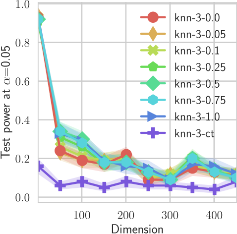
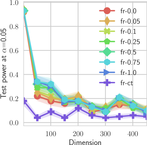
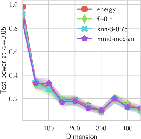
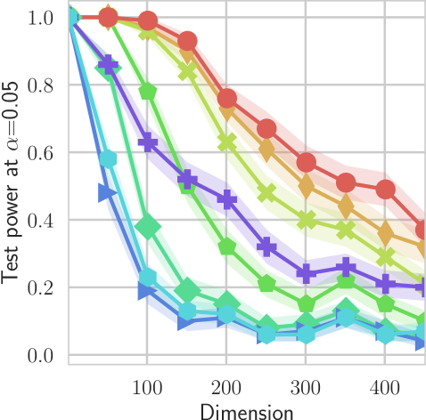
Power as a function of and .
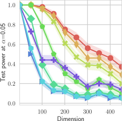
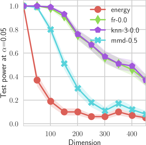
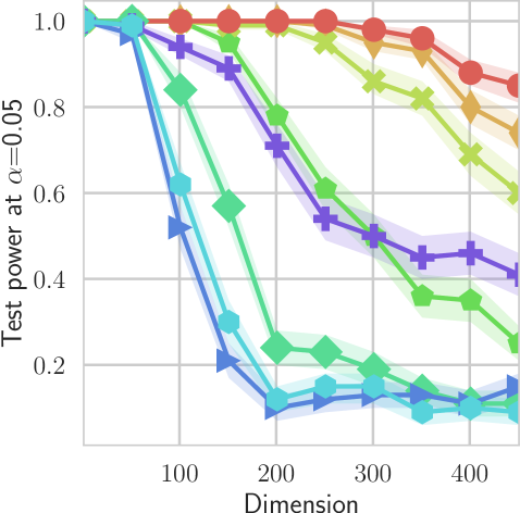
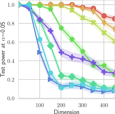
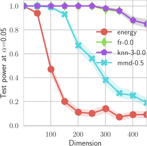
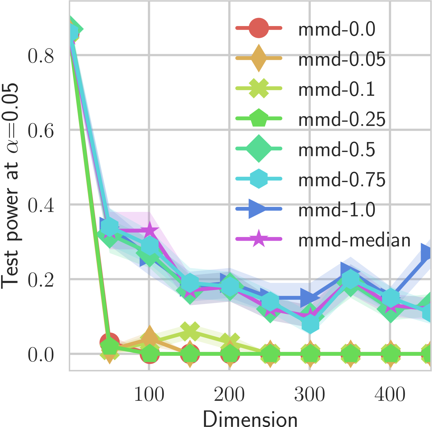
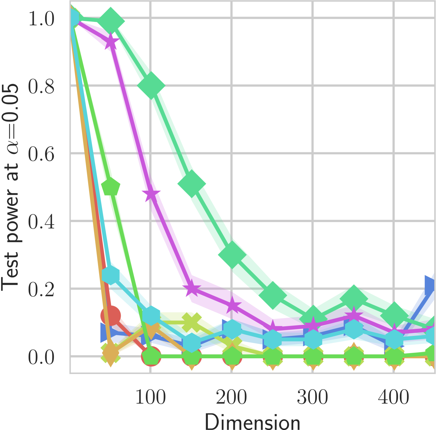
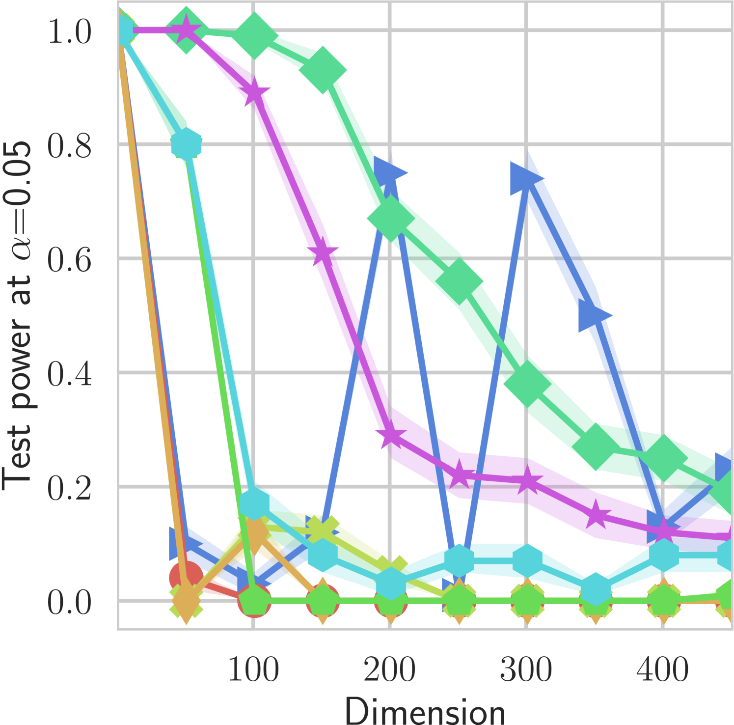
In our first experiment we analyze the effect of the smoothing strength on the power of our differentiable tests. In addition to the classical FR and -NN tests, we have considered the unbiased MMD test [9] with the squared exponential kernel (as implemented in Shogun [37] using the code from [12]), and the energy test [13]. The problem that we consider, which is challenging in high dimensions, is that of differentiating the distribution from . This setting was considered to be fair in [38], as the KL divergence between the distribution is constant irrespective of the dimension. To set the smoothing strength and the bandwidth of the MMD kernel (in addition to the median heuristic) we used the same strategy as in [38] by setting for varying . The results are presented in Figure 2, where can observe that (i) our test have similar results with MMD for shift-alternatives, while performing significantly better for scale alternatives, and (ii) by varying the smoothing parameter we can significantly increase the power of the test. In the third column we present only the best performing MMD, while we present the remaining results in Appendix B. Note that we expect the power to go to zero as the dimension increases [7, 38].
Learning.
As we have already hinted in the introduction, we stochastically optimize
using the Adam [39] optimizer. To optimize, we draw at each round samples from the true distribution , samples from the base measure , and then plug them in into the smoothed -statistic.
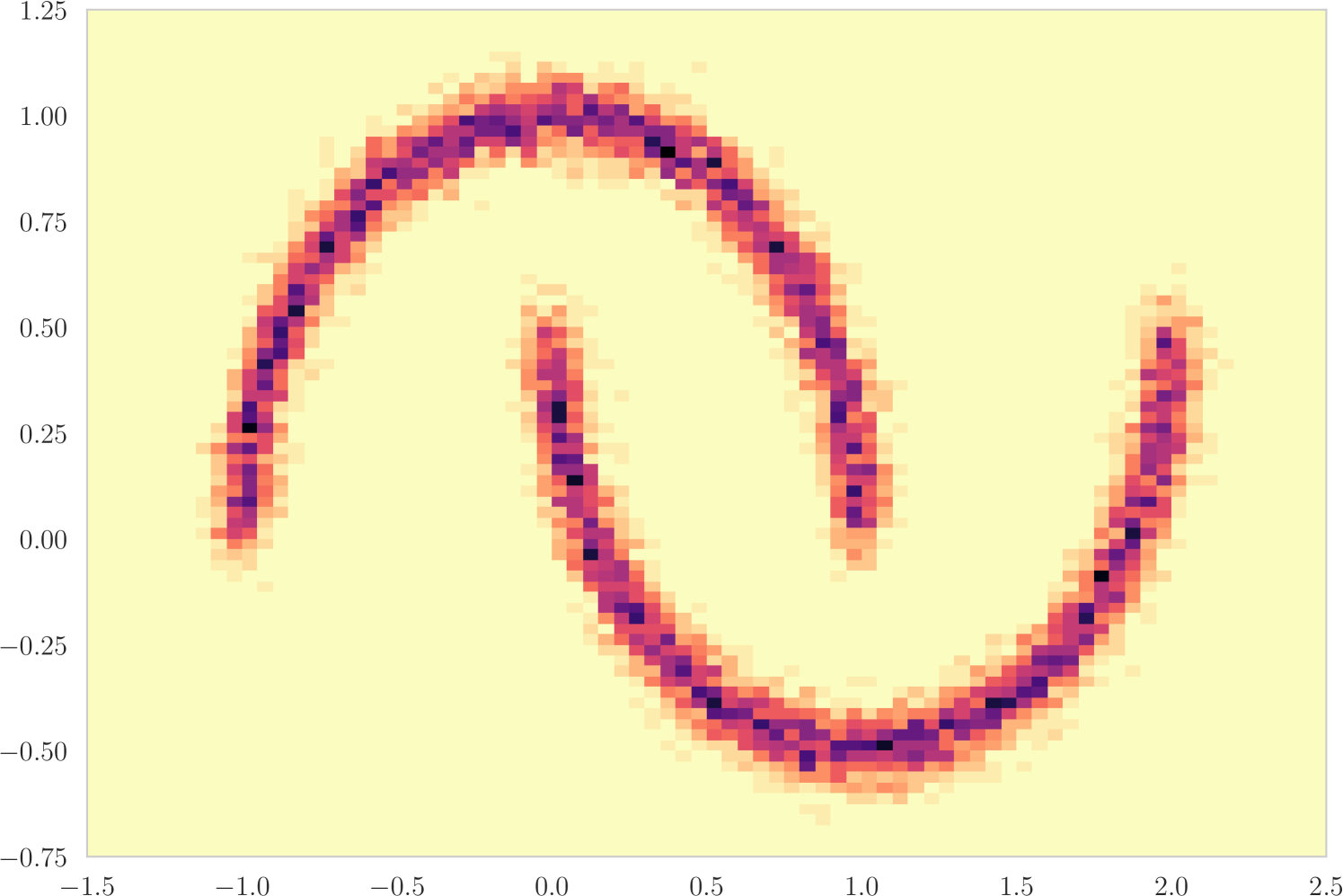
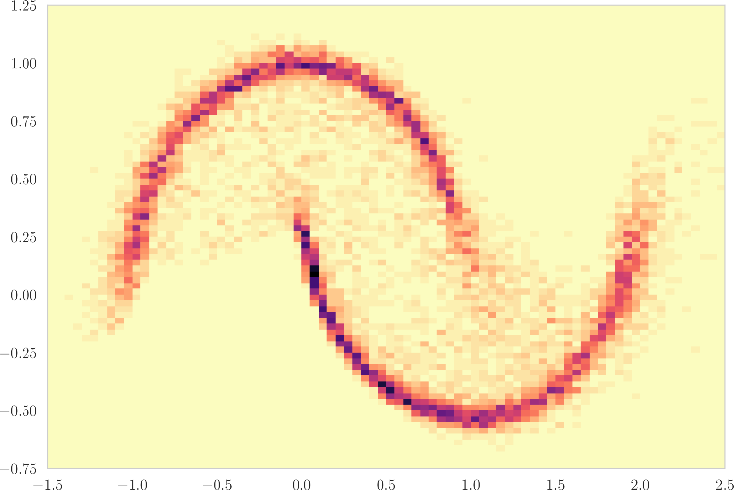
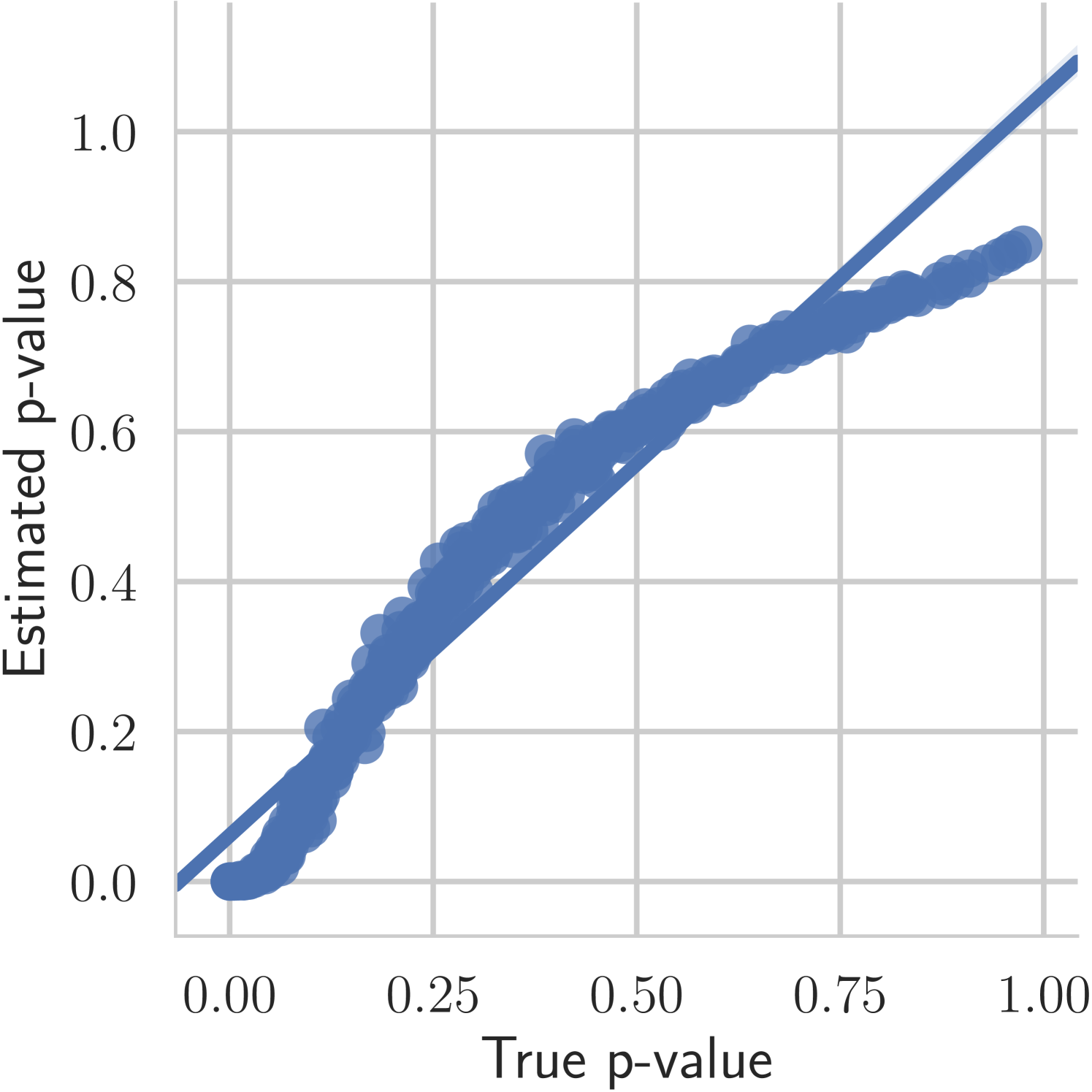
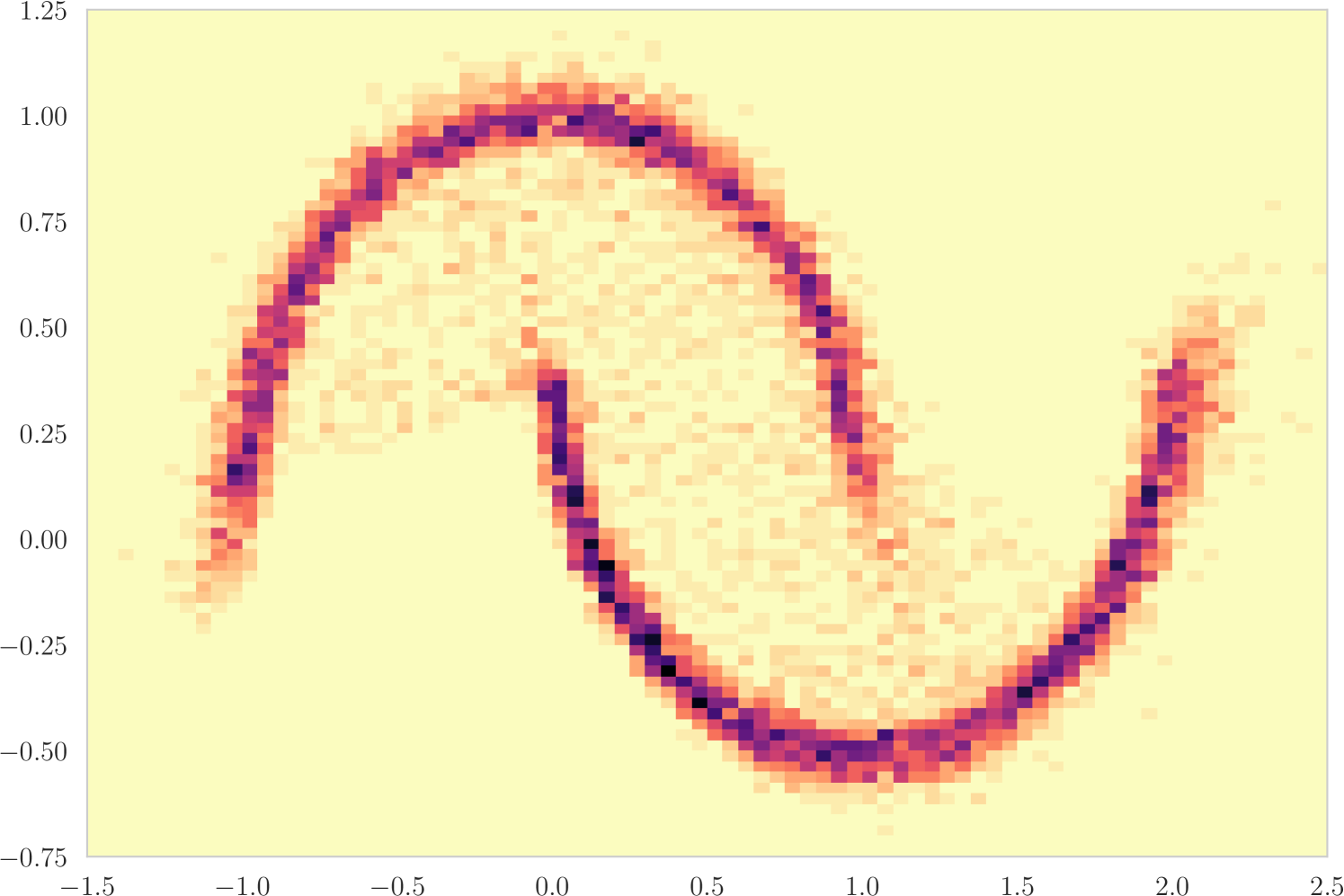
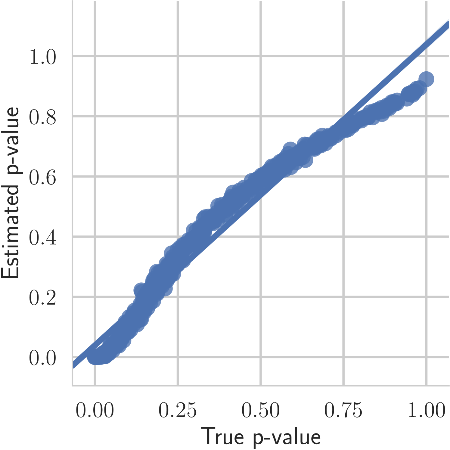
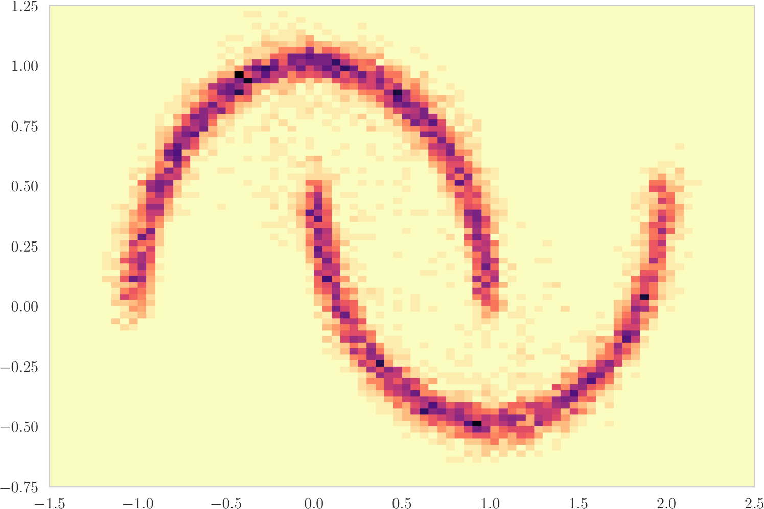
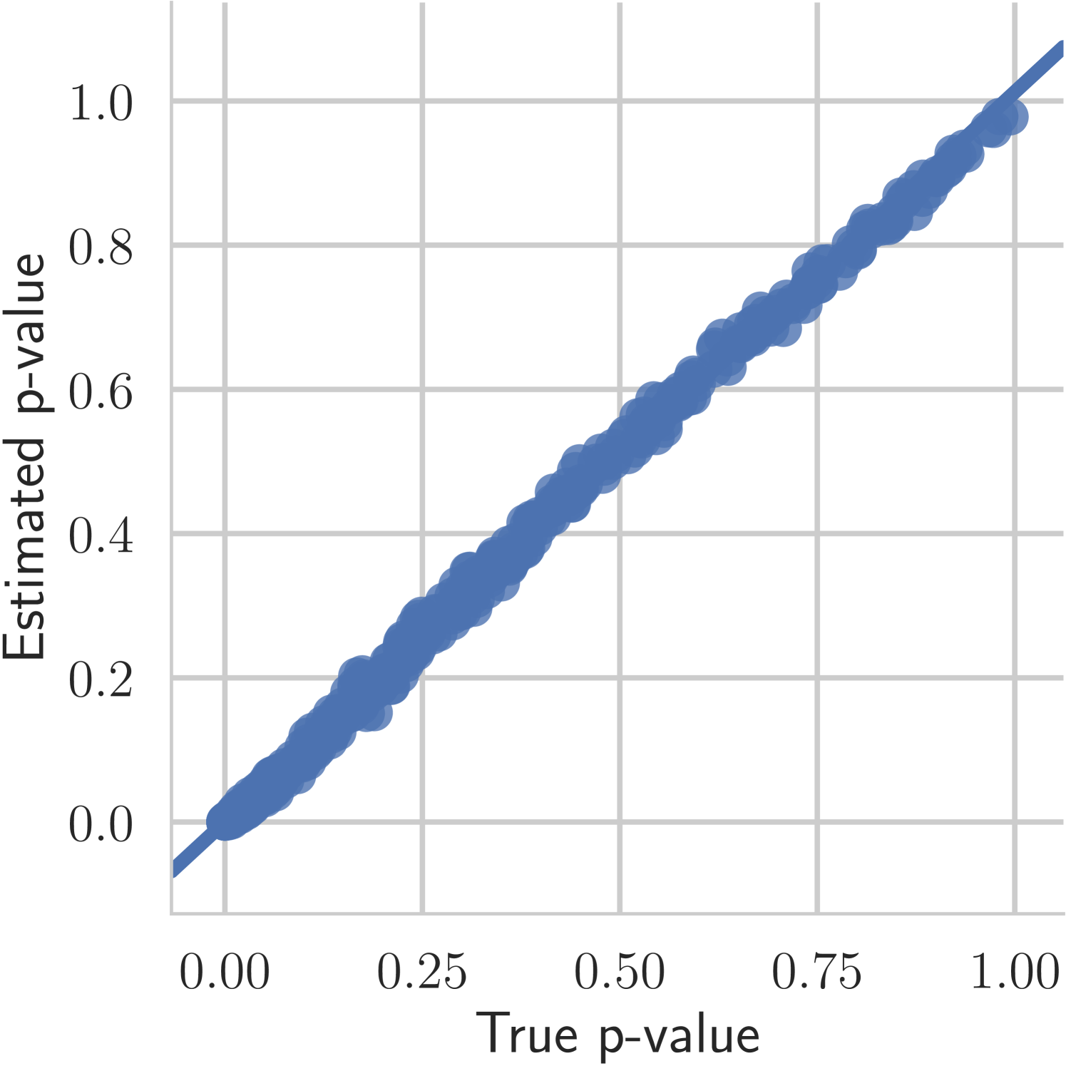
The first experiment we perform, with the goal of understanding the effects of , is on the toy two moons dataset from scikit-learn [40]. We show the results in Figure 3. From the second row, showing the estimated -value versus the correct one (from 1000 random permutations) at several points during training, we can indeed see that the permutation null gets closer to normality as decreases. Most importantly, note that the relationship is monotone, so that we would expect the optimization to not be significantly harmed if we use the approximation. Qualitatively, we can observe that the solutions have the general structure of , and that they improve as we decrease — the symmetry is better captured and the two moons get better separated.
MNIST.
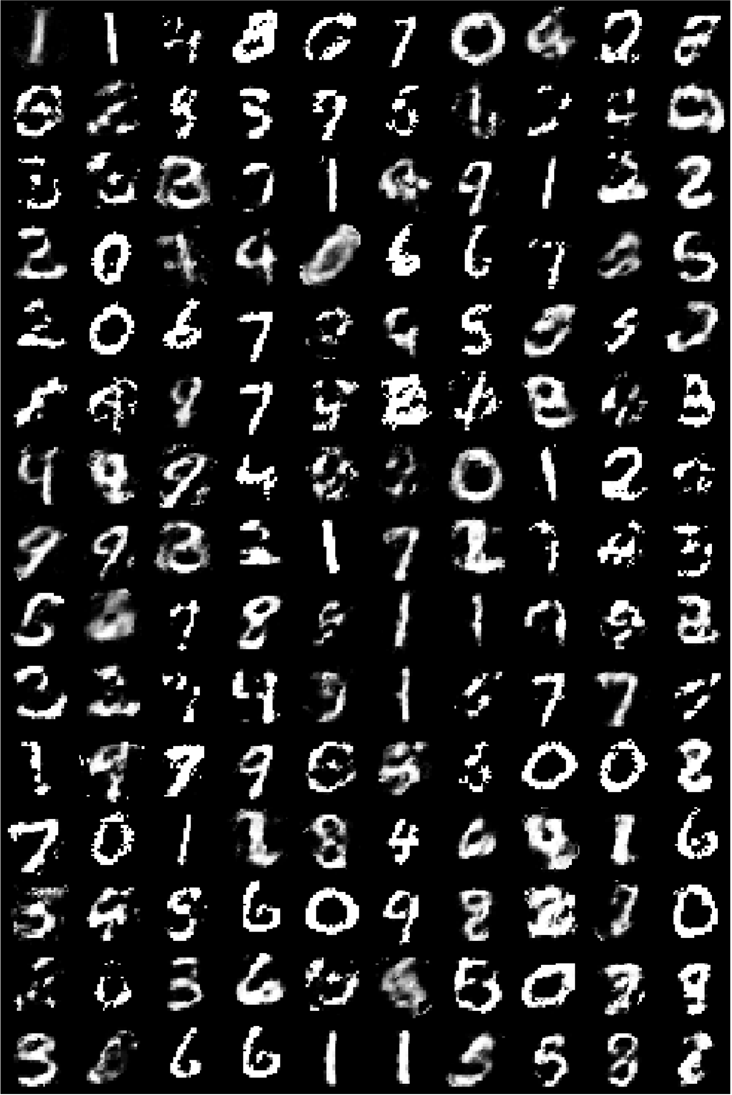
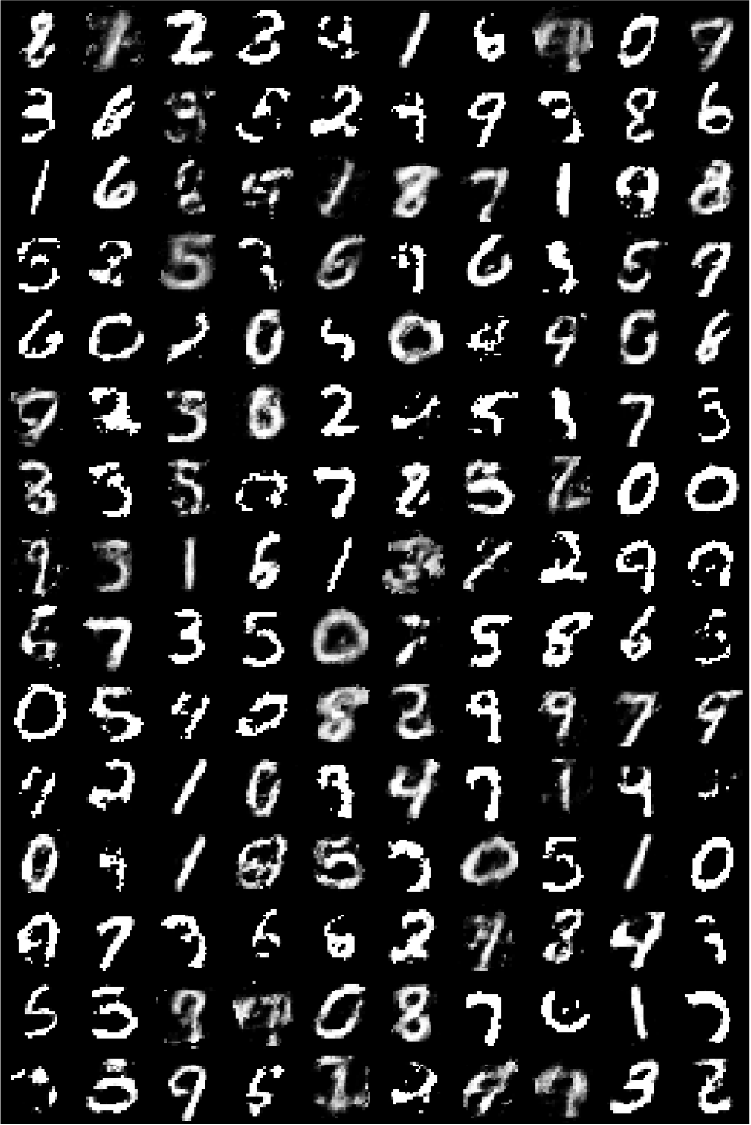
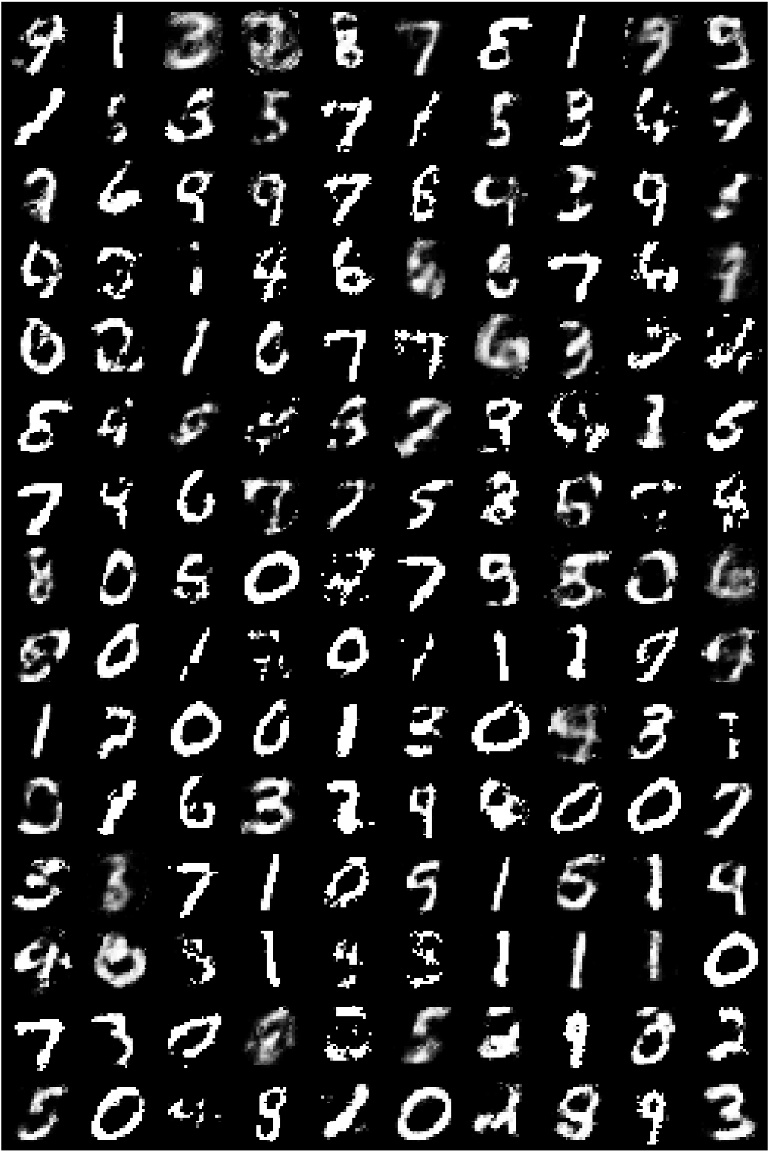
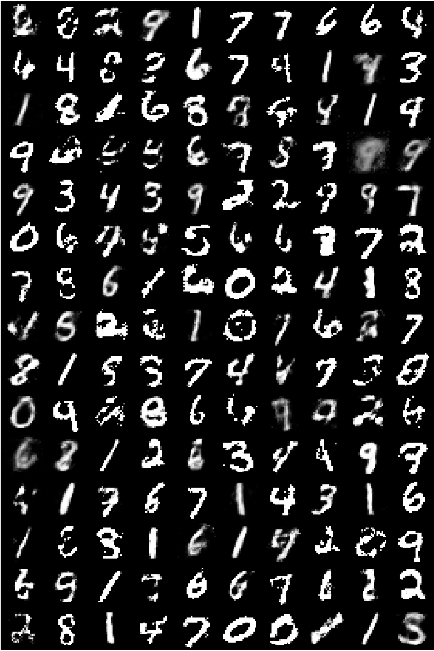
Finally, we have trained several models on the MNIST [41] dataset, which we present in Figure 4. We can observe that despite the high (784) dimensional data and the fact that we use the distance directly on the pixels, the learned models generate digits that look mostly realistic and are competitive with those obtained using MMD [10, 11].
6 Conclusion
We have developed smoothed two-sample graph tests that can be used for learning implicit models. These tests moreover outperform their classical equivalents on the problem of two sample testing. We have shown how to compute them by performing inference in undirected models, and presented alternative interpretations by drawing connections to neighbourhood component analysis and spectral graph sparsifiers. In the last section we have experimentally showcased the benefits of our approach, and presented results from a learned model.
Acknowledgements.
The research was partially supported by ERC StG 307036 and a Google European PhD Fellowship.
References
- Wald and Wolfowitz [1940] Abraham Wald and Jacob Wolfowitz. On a test whether two samples are from the same population. Annals of Mathematical Statistics, 11(2):147–162, 1940.
- Friedman and Rafsky [1979] Jerome H Friedman and Lawrence C Rafsky. Multivariate generalizations of the wald-wolfowitz and smirnov two-sample tests. Annals of Statistics, pages 697–717, 1979.
- Friedman and Rafsky [1983] Jerome H Friedman and Lawrence C Rafsky. Graph-theoretic measures of multivariate association and prediction. Annals of Statistics, pages 377–391, 1983.
- Henze and Penrose [1999] Norbert Henze and Mathew D Penrose. On the multivariate runs test. Annals of Statistics, pages 290–298, 1999.
- Henze [1988] Norbert Henze. A multivariate two-sample test based on the number of nearest neighbor type coincidences. Annals of Statistics, pages 772–783, 1988.
- Schilling [1986] Mark F Schilling. Multivariate two-sample tests based on nearest neighbors. Journal of the American Statistical Association, 81(395):799–806, 1986.
- Bhattacharya [2015] Bhaswar B Bhattacharya. Power of graph-based two-sample tests. arXiv preprint arXiv:1508.07530, 2015.
- Chen and Zhang [2013] Hao Chen and Nancy R Zhang. Graph-based tests for two-sample comparisons of categorical data. Statistica Sinica, pages 1479–1503, 2013.
- Gretton et al. [2012] Arthur Gretton, Karsten M Borgwardt, Malte J Rasch, Bernhard Schölkopf, and Alexander Smola. A kernel two-sample test. Journal of Machine Learning Research, 13(Mar):723–773, 2012.
- Li et al. [2015] Yujia Li, Kevin Swersky, and Rich Zemel. Generative moment matching networks. In International Conference on Machine Learning (ICML), 2015.
- Dziugaite et al. [2015] Gintare Karolina Dziugaite, Daniel M. Roy, and Zoubin Ghahramani. Training generative neural networks via maximum mean discrepancy optimization. In Uncertainty in Artificial Intelligence (UAI), 2015.
- Sutherland et al. [2016] Dougal J Sutherland, Hsiao-Yu Tung, Heiko Strathmann, Soumyajit De, Aaditya Ramdas, Alex Smola, and Arthur Gretton. Generative models and model criticism via optimized maximum mean discrepancy. In International Conference on Learning Representations (ICLR), 2016.
- Székely and Rizzo [2013] Gábor J Székely and Maria L Rizzo. Energy statistics: A class of statistics based on distances. Journal of Statistical Planning and Inference, 143(8):1249–1272, 2013.
- Bellemare et al. [2017] Marc G Bellemare, Ivo Danihelka, Will Dabney, Shakir Mohamed, Balaji Lakshminarayanan, Stephan Hoyer, and Rémi Munos. The cramer distance as a solution to biased wasserstein gradients. arXiv preprint arXiv:1705.10743, 2017.
- Sugiyama et al. [2012] Masashi Sugiyama, Taiji Suzuki, and Takafumi Kanamori. Density ratio estimation in machine learning. Cambridge University Press, 2012.
- Goodfellow et al. [2014] Ian Goodfellow, Jean Pouget-Abadie, Mehdi Mirza, Bing Xu, David Warde-Farley, Sherjil Ozair, Aaron Courville, and Yoshua Bengio. Generative adversarial nets. In Advances in Neural Information Processing Systems (NIPS), pages 2672–2680, 2014.
- Salimans et al. [2016] Tim Salimans, Ian Goodfellow, Wojciech Zaremba, Vicki Cheung, Alec Radford, and Xi Chen. Improved techniques for training gans. In Advances in Neural Information Processing Systems (NIPS), pages 2234–2242, 2016.
- Nowozin et al. [2016] Sebastian Nowozin, Botond Cseke, and Ryota Tomioka. -GAN: Training generative neural samplers using variational divergence minimization. In Advances in Neural Information Processing Systems (NIPS), pages 271–279, 2016.
- Ali and Silvey [1966] Syed Mumtaz Ali and Samuel D Silvey. A general class of coefficients of divergence of one distribution from another. Journal of the Royal Statistical Society. Series B (Methodological), pages 131–142, 1966.
- Mohamed and Lakshminarayanan [2016] Shakir Mohamed and Balaji Lakshminarayanan. Learning in implicit generative models. arXiv preprint arXiv:1610.03483, 2016.
- Prim [1957] Robert Clay Prim. Shortest connection networks and some generalizations. Bell Labs Technical Journal, 36(6):1389–1401, 1957.
- Kruskal [1956] Joseph B Kruskal. On the shortest spanning subtree of a graph and the traveling salesman problem. Proceedings of the American Mathematical society, 7(1):48–50, 1956.
- Berisha and Hero [2015] Visar Berisha and Alfred O Hero. Empirical non-parametric estimation of the fisher information. IEEE Signal Processing Letters, 22(7):988–992, 2015.
- Wainwright and Jordan [2008] Martin J Wainwright and Michael I Jordan. Graphical models, exponential families, and variational inference. Foundations and Trends® in Machine Learning, 1(1-2), 2008.
- Daniels [1944] Henry E Daniels. The relation between measures of correlation in the universe of sample permutations. Biometrika, 33(2):129–135, 1944.
- Barbour and Eagleson [1986] AD Barbour and GK Eagleson. Random association of symmetric arrays. Stochastic Analysis and Applications, 4(3):239–281, 1986.
- Yukich [2006] Joseph E Yukich. Probability theory of classical Euclidean optimization problems. Springer, 2006.
- Tarlow et al. [2012] Daniel Tarlow, Kevin Swersky, Richard S Zemel, Ryan Prescott Adams, and Brendan J Frey. Fast exact inference for recursive cardinality models. Uncertainty in Artificial Intelligence (UAI), 2012.
- Swersky et al. [2012] Kevin Swersky, Ilya Sutskever, Daniel Tarlow, Richard S Zemel, Ruslan R Salakhutdinov, and Ryan P Adams. Cardinality restricted boltzmann machines. In Advances in Neural Information Processing Systems (NIPS), pages 3293–3301, 2012.
- Goldberger et al. [2005] Jacob Goldberger, Geoffrey E Hinton, Sam T Roweis, and Ruslan R Salakhutdinov. Neighbourhood components analysis. In Advances in Neural Information Processing Systems (NIPS), pages 513–520, 2005.
- Tarlow et al. [2013] Daniel Tarlow, Kevin Swersky, Laurent Charlin, Ilya Sutskever, and Rich Zemel. Stochastic k-neighborhood selection for supervised and unsupervised learning. In International Conference on Machine Learning, pages 199–207, 2013.
- Lyons [2003] Russell Lyons. Determinantal probability measures. Publications mathématiques de l’IHÉS, 98(1):167–212, 2003.
- Chandra et al. [1996] Ashok K Chandra, Prabhakar Raghavan, Walter L Ruzzo, Roman Smolensky, and Prasoon Tiwari. The electrical resistance of a graph captures its commute and cover times. Computational Complexity, 6(4):312–340, 1996.
- Spielman and Srivastava [2011] Daniel A Spielman and Nikhil Srivastava. Graph sparsification by effective resistances. SIAM Journal on Computing, 40(6):1913–1926, 2011.
- Spielman and Teng [2014] Daniel A Spielman and Shang-Hua Teng. Nearly linear time algorithms for preconditioning and solving symmetric, diagonally dominant linear systems. SIAM Journal on Matrix Analysis and Applications, 35(3):835–885, 2014.
- Spielman and Teng [2011] Daniel A Spielman and Shang-Hua Teng. Spectral sparsification of graphs. SIAM Journal on Computing, 40(4):981–1025, 2011.
- Sonnenburg et al. [2010] SĆ Sonnenburg, Sebastian Henschel, Christian Widmer, Jonas Behr, Alexander Zien, Fabio de Bona, Alexander Binder, Christian Gehl, VojtÄ Franc, et al. The shogun machine learning toolbox. Journal of Machine Learning Research, 11(Jun):1799–1802, 2010.
- Ramdas et al. [2015] Aaditya Ramdas, Sashank Jakkam Reddi, Barnabás Póczos, Aarti Singh, and Larry A Wasserman. On the decreasing power of kernel and distance based nonparametric hypothesis tests in high dimensions. In AAAI, 2015.
- Kingma and Ba [2015] Diederik Kingma and Jimmy Ba. Adam: A method for stochastic optimization. In International Conference on Learning Representations (ICLR), 2015.
- Pedregosa et al. [2011] F. Pedregosa, G. Varoquaux, A. Gramfort, V. Michel, B. Thirion, O. Grisel, M. Blondel, P. Prettenhofer, R. Weiss, V. Dubourg, J. Vanderplas, A. Passos, D. Cournapeau, M. Brucher, M. Perrot, and E. Duchesnay. Scikit-learn: Machine learning in Python. Journal of Machine Learning Research, 12:2825–2830, 2011.
- LeCun et al. [1998] Yann LeCun, Léon Bottou, Yoshua Bengio, and Patrick Haffner. Gradient-based learning applied to document recognition. Proceedings of the IEEE, 86(11):2278–2324, 1998.
Appendix A Proofs
Proof of 3.
The expectation of the statistic under is (when is a uniformly random labelling)
where the inner expectation has been computed in [2]. We can also easily compute the variance as
| (5) |
∎
Proof of 2.
We can split the sum in the variance formula over all edge pairs into three groups as follows
| (6) |
where sums over all edges that share at least one vertex with , and sums over those edges that share no vertex with , and denote the reverse edge of (if it exist, zero otherwise). Note that each term appears twice if , as in the formula for the variance (5). Moreover, note that if , then in the above formula the term (same for ) gets multiplied by , as it appears in both the first and the third term. Given that assumption that under , we also know that
so that eq. (6) can be simplified to
which be simplified to
Now the result follows by observing that
To understand why this holds, let us count how many times each term appears on both sides of the equality if we expand the lhs. If and they share exactly one vertex, then the lhs will have two terms, as and will be multiplied only at the term corresponding to the shared vertex. On the other hand, if we will again have two terms, as we get one contribution from each end-point of . Finally, if , we have a total of four terms, as we get two from each end-point. Thus, eq. (6) is equal to
Finally, if we subtract and simplify the expression we have
which is exactly what is claimed in the theorem, if we observe that and are the only edges parallel to . ∎
Proof that when .
First, note that , if and only if , which is equivalent to . Similarly, we have iff , which can be re-written as , i.e., . Combining these two inequalities proves the result.
Proof of 4.
Let us compute an upper bound on the quantities in [26].
Then, the upper bound has the form
which can be simplified to
which is what is claimed in the theorem.
Appendix B Experiments
B.1 MMD
B.2 Architecture
We have used the same architecture as in [10, 12], which using the modules from PyTorch can be written as follows.
nn.Sequential(
    nn.Linear(noise_dim, 64),
    nn.ReLU(),
    nn.Linear(64, 256),
    nn.ReLU(),
    nn.Linear(256, 256),
    nn.ReLU(),
    nn.Linear(256, 1024),
    nn.ReLU(),
    nn.Linear(1024, ambient_dim))
For MNIST we have also added a terminal nn.Tanh layer.
B.3 Data
We have used the MNIST data as packaged by torchvision, with the additional processing of scaling the output to as we are using a final Tanh layer. For the two moons data, we have used a noise level of .
B.4 Optimization
All details are provided in the table below. In some cases we have optimized with a larger step for a number of epochs, and then reduced it for the remaining epochs — in the table below these are separated by commas.
| Model | Step size | Batch size | Epochs |
|---|---|---|---|
| Figure 3(b) | 256 | 500 | |
| Figure 3(c) | 256 | 500 | |
| Figure 3(d) | 256 | 500 | |
| Figure 4(a) | 256 | 500, 500 | |
| Figure 4(b) | 512 | 500, 500 | |
| Figure 4(c) | 128 | 100, 100 | |
| Figure 4(d) | 128 | 100, 100 |