Learning Interpretable Error Functions
for Combinatorial Optimization Problem Modeling
Abstract
In Constraint Programming, constraints are usually represented as predicates allowing or forbidding combinations of values. However, some algorithms exploit a finer representation: error functions. Their usage comes with a price though: it makes problem modeling significantly harder. Here, we propose a method to automatically learn an error function corresponding to a constraint, given a function deciding if assignments are valid or not. This is, to the best of our knowledge, the first attempt to automatically learn error functions for hard constraints. Our method uses a variant of neural networks we named Interpretable Compositional Networks, allowing us to get interpretable results, unlike regular artificial neural networks. Experiments on 5 different constraints show that our system can learn functions that scale to high dimensions, and can learn fairly good functions over incomplete spaces.
1 Introduction
Twenty years separate Freuder’s papers Freuder (1997) and Freuder (2018), both about the grand challenges Constraint Programming (CP) must tackle “to be pioneer of a new usability science and to go on to engineering usability” Freuder (2007). To respond to the lack of a “Model and Run” approach in CP Puget (2004); Wallace (2003), several languages have been developed since the late 2000’s, such as ESSENCE Frisch et al. (2008), XCSP Boussemart et al. (2016) or MiniZinc Nethercote et al. (2007). However, they require users to have deep expertise on global constraints and to know how well these constraints, and their associated mechanisms such as propagators, are suiting the solver. We are still far from the original Holy Grail of CP: “the user states the problem, the computer solves it” Freuder (1997).
This paper makes a contribution in automatic CP problem modeling. We focus on Error Function Satisfaction and Optimization Problems we defined in the next section. Compare to classical Constraint Satisfaction and Constrained Optimization Problems, they rely on a finer structure about the problem: the cost functions network, which is, for this work, an ordered structure over invalid assignments that constraint solver can exploit efficiently to improve the search.
In this paper, we propose a method to learn error functions automatically; a direction that, to the best of our knowledge, had not been explored in Constraint Programming. We focus here on “easy-to-use” aspects of Constraint Programming.
To sum up, the main contributions of this paper are: 1. to give the first formal definition of Error Function Satisfaction Problems and Error Function Optimization Problems, 2. to introduce Interpretable Compositional Networks, a variant of neural networks to get interpretable results, 3. to propose an architecture of Interpretable Compositional Network to learn error functions, and 4. to provide a proof of concept by learning Interpretable Compositional Network models of error functions, using a genetic algorithm, and to show that most of models give scalable functions, and remain fairly effective using incomplete training sets.
2 Error Function and Optimization Problems
Constraint Satisfaction Problem (CSP) and Constrained Optimization Problem (COP) are hard constraint-based problems defined upon a classical constraint network, where constraints can be seen as predicates allowing or forbidding some combinations of variable assignments.
Likewise, Error Function Satisfaction Problem (EFSP) and Error Function Optimization Problem (EFOP) are hard constraint-based problems defined upon a specific constraint network named cost function network Cooper et al. (2020). Constraints are then represented by cost functions , where is the domain of -th variable in the constraint scope, the number of variables (i.e., the size of this scope) and the set of possible costs.
A cost function network is a quadruplet where is a set of variables, the set of domains for each variable, i.e., the sets of values each variable can take, the set of cost functions and a cost structure. A cost structure is also a quadruplet with the totally ordered set of possible costs, a commutative, associative, and monotone aggregation operator and and the neutral and absorbing elements of , respectively.
In Constraint Programming, cost functions are often associated to soft constraints: they can be interpreted as preferences over valid or acceptable assignments. However, this is not necessarily the case: it depends on the cost structure. For instance, the classical cost structure
makes the cost function network equivalent to a classical constraint network, so dealing with hard constraints.
Here, we consider particular cost functions that represent hard constraints only, by considering the additive cost structure . The additive cost structure produces useful cost function networks capturing problems such as Maximum Probability Explanation (MPE) in Bayesian networks and Maximum A Posteriori (MAP) problems in Markov random fields Hurley et al. (2016).
In this paper, an error function is a cost function defined in a cost function network with the additive cost structure . Intuitively, error functions are preferences over invalid assignments. Let be an error function representing a constraint and be an assignment of variables in the scope of . Then iff satisfies the constraint . For all invalid assignments , such that the closer is to 0, the closer is to satisfy .
The goal of this paper is not to study the advantages of such cost function networks over regular constraint networks. Without formally defining EFSP and EFOP problems, some studies illustrate that solvers (in particular, metaheuristics) can exploit this structure efficiently leading to state-of-the-art experimental results, both in sequential Codognet and Diaz (2001) and parallel solving Caniou et al. (2015). In addition, our Experiment 3 shows that error functions representing the classic AllDifferent constraint gives models that clearly outperformed a model based on a regular constraint networks in terms of runtimes, for models with either hand-crafted or learned error functions.
Let be a variable assignment, and denote by the projection of over variables in the scope of a constraint . We can now define the EFSP and EFOP problems.
-
Problem: Error Function Satisfaction Problem
Input: A cost function network .
Question: Does a variable assignment exist such that holds?
-
Problem: Error Function Optimization Problem
Input: A cost function network and an objective function .
Question: Find a variable assignment maximizing or minimizing the value of such that holds.
With the system we propose in this paper, users provide the usual constraint network , and it computes the equivalent cost function networks . Learned error functions composing the set are independent of the number of variables in constraints scope, and are expressed in an interpretable way: users can understand these functions and easily modify them at will. This way, users can have the power of EFSP and EFOP with the same modeling effort as for CSP and COP.
3 Related works
This work belongs to one of the three directions identified by Freuder Freuder (2007): Automation, i.e., “automating efficient and effective modeling and solving”. To the best of our knowledge, few efforts have been done on the modeling side.
Another of these three directions which is slightly related is Acquisition described by Freuder to be “acquiring a complete and correct representation of real problems”. Remarkable efforts on this topic have been done by Bessiere’s research team, for instance with constraints learning by induction from positive and negative examples Bessiere et al. (2005) and with interactive queries asked to users Bessiere et al. (2007), and with constraint network learning also through with interactive queries Bessiere et al. (2013).
Model Seeker Beldiceanu and Simonis (2012) is a passive learning system taking positive examples only, which are certainly easier for users to provide. It transforms examples into data adapted to the Global Constraint Catalog Beldiceanu et al. (2007), then generate and simplify candidates by eliminating dominated ones. Model Seeker is particularly efficient to find a good inner structure of the target constraint network.
Teso Teso (2019) gives a good survey on Constraint Learning with this interesting remark: “A major bottleneck of [constraint-based problem modeling] is that obtaining a formal constraint theory is non-obvious: designing an appropriate, working constraint satisfaction or optimization problem requires both domain and modeling expertise. For this reason, in many cases a modeling expert is hired and has to interact with domain expert to acquire informal requirements and turn them into a valid constraint theory. This process can be expensive and time-consuming.”
We can consider that Constraint Acquisition, or Constraint Learning, focuses on modeling expertise and puts domain expertise on background: users would not be able to understand and modify a learned model without the help of a modeling expert. The goal of these systems is mainly to simplify the interaction between the domain and the modeling experts.
Our work is taking the opposite direction: we focus on domain expertise and put modeling expertise on background. With our system, users always have the control over constraints’ representation, which can be modified at will to fit needs related to their domain expertise. Constraint Implementation Learning is what best describes this research topic.
4 Method design
The main result of this paper is to propose a method to automatically learn an error function representing a constraint, to make easier the modeling of EFSP/EFOP. We are tackling a regression problem since the goal is to find a function that outputs a target value. Before diving into the description of our method, we need to introduce some essential notions.
4.1 Definitions
We propose a method to automatically learn an error function from the concept of a constraint. As described in Bessiere et al. Bessiere et al. (2017), the concept of a constraint is a Boolean function that, given an assignment , outputs true if satisfies the constraint, and false otherwise. Concepts are the predicate representation of constraints referred at the beginning of Section 2.
Our method learns error functions in a supervised fashion, searching for a function computing the Hamming cost of each assignment. The Hamming cost of an assignment is the minimum number of variables in to reassign to get a solution, i.e., a variable assignment satisfying the considered constraint. If is a solution, then its Hamming cost is 0.
Given the number of variables of a constraint and their domain, the constraint assignment space is the set of couples where is an assignment and the Boolean output of the concept applied on . Such constraint assignment spaces can be generated from concepts. These spaces are said to be complete if and only if they contain all possible assignments, i.e., all combinations of possible values of variables in the scope of the constraint. Otherwise, spaces are said to be incomplete.
In this work, we consider an error function to be a (non-linear) combination of elementary operations. Complete spaces are intuitively good training sets since it is easy to compute the exact Hamming cost of their elements. We also consider assignments from incomplete spaces where their Hamming cost has been approximated regarding a subset of solutions in the constraint assignment space, in case the exact Hamming cost function is unknown.
4.2 Main result
To learn an error function as a non-linear combination of elementary operations, we propose a network inspired by Compositional Pattern-Producing Networks (CPPN). CPPNs Stanley (2007) are themselves a variant of artificial neural networks. While neurons in regular neural networks usually contain sigmoid-like functions only (such as ReLU, i.e. Rectified Linear Unit), CPPN’s neurons can contain many other kinds of function: sigmoids, Gaussians, trigonometric functions, and linear functions among others. CPPNs are often used to generate 2D or 3D images by applying the function modeled by a CPPN giving each pixel individually as input, instead of considering all pixels at once. This simple trick allows the learned CPPN model to produce images of any resolution.
We propose our variant by taking these two principles from CPPN: having neurons containing one operation among many possible ones, and handling inputs in a size-independent fashion. Due to their interpretable nature, we named our variant Interpretable Compositional Networks (ICN). In this paper, our ICNs are composed of four layers, each of them having a specific purpose and themselves composed of neurons applying a unique operation each. All neurons from a layer are linked to all neurons from the next layer. The weight on each link is purely binary: its value is either 0 or 1. This restriction is crucial to obtain interpretable functions. A weight between neurons and with the value 1 means that the neuron from layer takes as input the output of the neuron from layer . Weight with the value 0 means that discards the output of .
Here is our method workflow in 4 points:
1. Users provide a regular constraint network where is a set of concepts representing constraints.
2. For each constraint concept , we generate its ICN input space , which is either a complete or incomplete constraint assignment space. Those input spaces are our training sets. If the space is complete, then the Hamming cost of each assignment can be pre-computed before learning our ICN model. Otherwise, the incomplete space is composed of randomly drawn assignments and only an approximation of their Hamming cost can be pre-computed.
3. We learn the weights of our ICN model in a supervised fashion, with the following loss function:
| (1) |
where is the constraint assignment space, ICN () the output of the ICN model giving as an input, Hamming() the pre-computed Hamming cost of (only approximated if is incomplete), and R(ICN) is a regularization between 0 and 0.9 to favor short ICNs, i.e., with as few elementary operations as possible, such that .
4. We have hold-out test sets of assignments from larger dimensions to evaluate the quality of our learned error functions.
Notice we also have a hold-out validation set to fix the values of our hyperparameters, as described in Section 4.3.
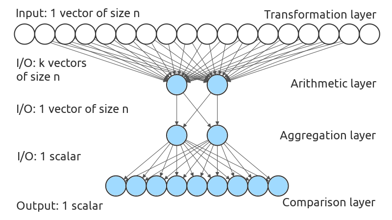
Figure 1 is a schematic representation of our network. It takes as input an assignment of variables, i.e., a vector of integers. The first layer, called transformation layer, is composed of 18 transformation operations, each of them applied element-wise on each element of the input vector. Such operations are for instance the maximum between the -th and -th elements of the input vector, or the number of -th elements of the vector smaller than the -th element such that holds. This layer is composed of both linear and non-linear operations. If an operation is selected (i.e., it has an outgoing weight equals to 1), it outputs a vector of integers.
If transformation operations are selected, then the next layer gets vectors of integers as input. This layer is the arithmetic layer. Its goal is to apply a simple arithmetic operation in a component-wise fashion on all -th element of our vectors to get one vector of integers at the end, combining previous transformations into a unique vector. We have considered only 2 arithmetic operations so far: the addition and the multiplication.
The output of the arithmetic layer is given to the aggregation layer. This layer crunches the whole vector into a unique integer. At the moment, the aggregation layer is composed of 2 operations: Sum computing the sum of input values and counting the number of input values strictly greater than 0.
Finally, the computed scalar is transmitted to the comparison layer with 9 operations. Examples of these operations are the identity, or the absolute value of the input minus a given parameter. This layer compares its input with an external parameter value, or the number of variables of the problem, or the domain size, among others.
All elementary operations in our model are generic: we do not choose them to fit one or several particular constraints. Due to the page limit, we cannot give a comprehensive list of the 18 transformation and 9 comparison operations here. Although an in-depth study of the elementary operations properties would be interesting, this is out of the scope of this paper: its goal is to show that learning interpretable error functions via a generic ICN is possible, and in the same way results with neural networks do not always use ReLU as an activation function, there is no reason to reduce ICN to its current 31 elementary operations or even a 4-layer architecture. Such elements can be changed by users to best fit their needs.
To have simple models of error functions, operations of the arithmetic, the aggregation, and the comparison layers are mutually exclusive, meaning that precisely one operation is selected for each of these layers. However, many operations from the transformation layer can be selected to compose the error function. Combined with the choice of having binary weights, it allows us to have a very comprehensible combination of elementary operations to model an error function, making it readable and intelligible by a human being. For instance, the most frequenly learned error function is for AllDifferent, and for LinearSum, i.e., the Euclidian division of by the maximal domain size, with a parameter equals to the right hand side constant of the linear equation. Thus, once the model of an error function is learned, users have the choice to run the network in a feed-forward fashion to compute the error function, or to re-implement it directly in a programming language. Users can use our system to find error functions automatically, but they can also use it as a decision support system to find promising error functions that they may modify and adapt by hand.
4.3 Learning with Genetic Algorithms
Like any neural network, learning an error function through an ICN boils down to learning the value of its weights. Many of our elementary operations are discrete, therefore are not differentiable. Then, we cannot use a back-propagation algorithm to learn the ICN’s weights. This is why we use a genetic algorithm for this task.
Since our weights are binary, we represent individuals of our genetic algorithm by a binary vector, each bit corresponding to one operation in the four layers indicating if the operation is selected to be part of the error function.
We randomly generate an initial population of 160 individuals, check and fix them if they do not satisfy the mutually exclusive constraint of the comparison layer. Then, we run the genetic algorithm to produce at most 800 generations before outputting its best individual according to our fitness function.
Our genetic algorithm is rather simple: The fitness function is the loss function of our supervised learning depicted by Equation 1. Selection is made by a tournament selection between 2 individuals. Variation is done by a one-point crossover operation and a one-flip mutation operation, both crafted to always produce new individuals verifying the mutually exclusive constraint of the comparison layer. The crossover rate is fixed at 0.4, and exactly one bit is mutated for each selected individual with a mutation rate of 1. Replacement is done by an elitist merge, keeping 17% of the best individuals from the old generation into the new one, and a deterministic tournament truncates the new population to 160 individuals. The algorithm stops before reaching 800 generations if no improvements have been done in the last 50 generations. We use the framework Evolving Objects Keijzer et al. (2002) to code our genetic algorithm.
Our hyperparameters, i.e., the population size, the maximal number of generations, the number of steady generations before early stop, the crossover, mutation and replacement rates, and the size of tournaments have been chosen using ParamILS Hutter et al. (2009), trained one week on one CPU over a large range of values for each hyperparameter. We use the same training instance used for Experiment 1, and new, larger instances as a hold-out validation set. These instances have been chosen because they are larger than our training instances and each of them contains about 45% of solutions, which is significantly less than the 1020% of solutions in training instances.
5 Experiments
To show the versatility of our method, we tested it on five very different constraints: AllDifferent, Ordered, LinearSum, NoOverlap1D, and Minimum. According to XCSP specifications Boussemart et al. (2016)222see also http://xcsp.org/specifications, those global constraints belong to four different families: Comparison (AllDifferent and Ordered), Counting/Summing (LinearSum), Packing/Scheduling (NoOverlap1D) and Connection (Minimum). Again according to XCSP specifications, these five constraints are among the twenty most popular and common constraints. We give a brief description of those five constraints below:
-
•
AllDifferent ensures that variables must all be assigned to different values.
-
•
LinearSum ensures that the equation holds, with the parameter a given integer.
-
•
Minimum ensures that the minimum value of an assignment verifies a given numerical condition. In this paper, we choose to consider that the minimum value must be greater than or equals to a given parameter .
-
•
NoOverlap1D is considering variables as tasks, starting from a certain time (their value) and each with a given length (their parameter). The constraint ensures that no tasks are overlapping, i.e., for all indexes with the number of variables, we have or . To have a simpler code, we have considered in our system that all tasks have the same length .
-
•
Ordered ensures that an assignment of variables must be ordered, given a total order. In this paper, we choose the total order . Thus, for all indexes , implies .
5.1 Experimental protocols
We conducted three experiments, with two of them requiring samplings. These samplings have been done using Latin hypercube sampling to have a good diversity among drawn assignments. When we need to sample the same number solutions and non-solutions, we draw assignments until we get of solutions and non-solutions.
Due to stochastic learning, all learning and testing have been done 100 times. We did not re-run batches of experiments to keep the ones with the best results, as it should always be the case with such experimental protocols.
All experiments have been done on a computer with a Core i9 9900 CPU and 32 GB of RAM, running on Ubuntu 20.04. Programs have been compiled with GCC with the 03 optimization option. Our entire system, its C++ source code, experimental setups, and the results files are accessible on GitHub333https://github.com/richoux/LearningErrorFunctions/tree/1.1 .
5.1.1 Experiment 1: scaling
The goal of this experiment is to show that learned error functions scale to high-dimensional constraints, indicating that learned error functions are independent of the size of the constraint scope.
For this experiment, error functions are learned upon a small, complete constraint assignment space, composed of about 500600 assignments and containing about 1020% of solutions. For each constraint, we run 100 error function learning over pre-computed complete constraint assignment space. Then, we compute the test error of these learned error functions over a sampled test set. Sampled test sets contain 10,000 solutions and 10,000 non-solutions, with 100 variables on domains of size 100, belonging to a constraint assignment space of size , thus greatly larger than training spaces containing 500600 assignments.
We show normalized mean training and test errors: first, we compute the mean error among all assignments composing the training or the test set. Then, we divide it by the number of variables composing the assignments. Indeed, having a mean error of 5 on assignments with 100 variables and 10 variables is significantly different: the first one indicates a mean error every 20 variables, the second a mean error one in two variables.
5.1.2 Experiment 2: learning over incomplete spaces
If, for any reasons, it is not possible to build a complete constraint assignment space, a robust system must be able to learn effective error functions upon large, incomplete spaces where the exact Hamming cost of their assignments is unknown.
In this experiment, we built pre-sampled training spaces by sampling 10,000 solutions and 10,000 non-solutions on large constraint assignment spaces of size between and , and with solution rates from % to %. Then, we approximate the Hamming cost of each non-solution by computing their Hamming distance with the closest solution among the 10,000 ones, and learn error functions on these 20,000 assignments and their estimated Hamming cost. Like for Experiment 1, we run 100 error functions learning of these pre-sampled incomplete spaces, so that each learning relies on the same training set. Finally, we evaluate the learned error functions over the same test sets than Experiment 1.
5.1.3 Experiment 3: learned error functions to solve problems
The goal of this experiment is to assess that learned error function can effectively be used to solve toy problems. Here, we use a local search solver to solve Sudoku.
Sudoku is a puzzle game where all numbers in the same row, the same column and the same sub-square must be different. There, it can be modeled as a satisfaction problem using the AllDifferent constraint only. We run 100 resolutions of random and Sudoku grids, with a timeout of 10 seconds. If no solutions have been found within 10 seconds, we consider the run to be unsolved.
We consider the mean and median run-time to compare different representations of the AllDifferent constraint. We have two baselines: 1., a pure CSP model where constraints are predicates, and 2., an EFSP model with an efficient hand-crafted error function representing AllDifferent. We compare those with two models using error functions learned with our system to represent AllDifferent: a., our EFSP model using the most frequently learned error function from the previous experiments and run through our neural network in a fast-forward fashion, and b., our EFSP model with the same error function but directly hard-coded in C++. The solver and its parameters remain the same: the only thing that is modified in these four different models is the expression of the AllDifferent constraint.
5.2 Results
5.2.1 Experiments 1 & 2
Table 1 shows the training errors of Experiment 1, where error functions have been learned 100 times for each constraint. The first column contains the normalized mean training error of the most frequently learned error function among the 100 runs, with its frequency in parenthesis. Next columns concern the median, the mean and the standard deviation.
Table 2 contains the normalized mean test errors of error functions learned with Experiments 1 and 2, with their median, mean and standard deviation. The normalized mean test error of the most frequently learned error function for each constraint in each experiment has been isolated in the first column of number, for comparison.
Comparing Table 1 and the first half of Table 2 lead us to conclude that our system is able to learn error functions that scale for most constraint, namely AllDifferent, LinearSum and Minimum. Their median training errors in Table 1 are perfect of almost perfect, so as their median test errors on greatly larger constraint assignment spaces.
Results are not as good for NoOverlap1D and Ordered, which are clearly the most intrinsically combinatorial constraints among our five ones. One could think that our system is overfitting on its training set, but results from Experiment 2 lead us to another conclusion.
To see this, let’s observe these Experiment 2’s results by comparing the first and the second half of Table 2. Error functions learned over incomplete training spaces are as good as the ones learned over small complete spaces for LinearSum and Minimum. We observe significant improvements of the median and the mean for NoOverlap1D (36.07% and 55.76%) and Ordered (52.83% and 49.05%). This is due not because error functions from Experiment 1 were overfitting, but because spaces from Experiment 1 were too small for these highly combinatorial constraints, containing too few different combinations and Hamming cost patterns.
| Constraints | most (freq.) | median | mean | std dev. |
|---|---|---|---|---|
| AllDifferent | 0 (98) | 0 | 5.001 | 35.185 |
| LinearSum | 0.004 (48) | 0.059 | 0.032 | 0.027 |
| Minimum | 0 (71) | 0 | 0.026 | 0.044 |
| NoOverlap | 0.039 (32) | 0.074 | 0.074 | 0.030 |
| Ordered | 0.020 (100) | 0.020 | 0.020 | 0 |
| Exp. | Constraints | most freq | median | mean | std dev |
|---|---|---|---|---|---|
| 1 | AllDifferent | 0 | 0 | 0.017 | 0.119 |
| LinearSum | 3 | 0.019 | 0.179 | 0.341 | |
| Minimum | 0 | 0 | 1.435 | 4.866 | |
| NoOverlap | 0.268 | 0.316 | 0.486 | 0.682 | |
| Ordered | 0.106 | 0.106 | 0.106 | 0 | |
| 2 | AllDifferent | 0.052 | 0.052 | 0.052 | 0 |
| LinearSum | 3 | 3 | 0.200 | 0.629 | |
| Minimum | 0 | 0 | 0.193 | 0.978 | |
| NoOverlap | 0.202 | 0.202 | 0.215 | 0.020 | |
| Ordered | 0.050 | 0.050 | 0.054 | 0.008 |
5.2.2 Experiment 3
The goal of this experiment is not to be state-of-the-art in terms of run-times for solving Sudoku, but to compare the average run-times of the same solver on four nearly identical Sudoku models presented in Section 5.1.3. For the model with a hand-crafted error function, we implemented the primal graph based violation error of AllDifferent from Petit et al. Petit et al. (2001). This function simply outputs the number of couples with identical values within a given assignment. To run this experiment, we used the framework GHOST from Richoux et al. Richoux et al. (2016), which includes a local search algorithm able to handle both CSP and EFSP models.
| Sudoku | Error Function | mean | median | std dev |
|---|---|---|---|---|
| nothing (CSP) | 624.41 | 217.21 | 1,1196.80 | |
| hand-crafted | 33.86 | 32.00 | 10.34 | |
| fast-forward | 55.57 | 49.27 | 41.17 | |
| hard-coded | 33.48 | 31.76 | 9.48 | |
| nothing (CSP) | - | - | - | |
| hand-crafted | 432.34 | 393.95 | 164.06 | |
| fast-forward | 825.61 | 774.36 | 271.09 | |
| hard-coded | 537.48 | 539.86 | 162.03 |
Table 3 shows that models with error functions clearly outperformed the model with the constraint represented as a predicate. Over 100 runs, no error function-based models hit the 10s timeout, but 4 runs of the regular constraint network model timed out on the grid, and all of them on the grid. Moreover, the learned error function hard-coded in C++ is nearly as efficient as the hand-crafted one (also coded in C++). The difference of runtimes between the learned error function hard-coded and computed through the ICN gives us an idea of the overhead of computing such a function through the ICN.
6 Discussions
Like Freuder Freuder (2007) wrote: “This research program is not easy because ’ease of use’ is not a science.” However, we believe our result is a step toward the ’ease of use’ of Constraint Programming, and in particular about EFSP and EFOP. Our system is excellent for learning error functions of simple constraints over complete spaces. For intrinsically combinatorial constraints, learning over large, incomplete spaces should be favored. One of the most significant results in this paper is that our system outputs interpretable results, unlike regular artificial neural networks. Error functions output by our system are intelligible. This allows our system to have two operating modes: 1. a fully automatic system, where error functions are learned and called within our system, being completely transparent to users who only need to furnish a concept function for each constraint, in addition to the regular sets of variables and domains , and 2. a decision support system, where users can look at a set of proposed error functions, pick up and modify the one they prefer.
The current limitation of our system is that it struggles to learn high-quality error function for very combinatorial constraints, such as Ordered and, in particular, NoOverlap1D. By combining results from Experiments 1 and 2, we can conclude that: 1. our system is not overfitting but need more diverse and expressive operations to learn a high-quality error function for such constraints, and 2. the Hamming cost is certainly not the better choice to represent their assignment error.
An extension of our work would be to do reinforcement learning rather than supervision learning based on the Hamming cost. Learning via reinforcement learning would allow finding error functions that are more adapted to the chosen solver.
References
- Beldiceanu and Simonis [2012] Nicolas Beldiceanu and Helmut Simonis. A model seeker: Extracting global constraint models from positive examples. In Principles and Practice of Constraint Programming (CP 2012), pages 141–157. Springer, 2012.
- Beldiceanu et al. [2007] Nicolas Beldiceanu, Mats Carlsson, Sophie Demassey, and Thierry Petit. Global constraint catalog: Past, present and future. Constraints, 12:21–62, 2007.
- Bessiere et al. [2005] Christian Bessiere, Remi Coletta, Frédéric Koriche, and Barry O’Sullivan. A sat-based version space algorithm for acquiring constraint satisfaction problems. In 16th European Conference on Machine Learning (ECML 2005), pages 23–34. Springer, 2005.
- Bessiere et al. [2007] Christian Bessiere, Remi Coletta, Barry O’Sullivan, and Mathias Paulin. Query-driven constraint acquisition. In Proceedings of the 20th International Joint Conference on Artificial Intelligence (IJCAI 2007), pages 50–55. IJCAI/AAAI Press, 2007.
- Bessiere et al. [2013] Christian Bessiere, Remi Coletta, Emmanuel Hebrard, George Katsirelos, Nadjib Lazaar, Nina Narodytska, Claude-Guy Quimper, and Toby Walsh. Constraint acquisition via partial queries. In Proceedings of the 23rd International Joint Conference on Artificial Intelligence (IJCAI 2013), pages 475–481. IJCAI/AAAI Press, 2013.
- Bessiere et al. [2017] Christian Bessiere, Frederic Koriche, Nadjib Lazaar, and Barry O’Sullivan. Constraint acquisition. Artificial Intelligence, 244:315–342, 2017.
- Boussemart et al. [2016] Frederic Boussemart, Christophe Lecoutre, Gilles Audemard, and Cédric Piette. XCSP3: An Integrated Format for Benchmarking Combinatorial Constrained Problems. arXiv e-prints, abs/1611.03398:1–238, 2016.
- Caniou et al. [2015] Yves Caniou, Philippe Codognet, Florian Richoux, Daniel Diaz, and Salvador Abreu. Large-scale parallelism for constraint-based local search: The costas array case study. Constraints, 20(1):30–56, 2015.
- Codognet and Diaz [2001] Philippe Codognet and Daniel Diaz. Yet another local search method for constraint solving. In International Symposium on Stochastic Algorithms: Foundations and Applications (SAGA 2001), pages 73–90. Springer, 2001.
- Cooper et al. [2020] Martin Cooper, Simon Givry, and Thomas Schiex. Valued constraint satisfaction problems. In A Guided Tour of Artificial Intelligence Research, volume 2, pages 185–207. Springer, 2020.
- Freuder [1997] Eugene C. Freuder. In pursuit of the holy grail. Constraints, 2(1):57–61, 1997.
- Freuder [2007] Eugene C. Freuder. Holy grail redux. Constraint Programming Letters, 1:3–5, 2007.
- Freuder [2018] Eugene C. Freuder. Progress towards the holy grail. Constraints, 23(2):158–171, 2018.
- Frisch et al. [2008] Alan Frisch, Warwick Harvey, Chris Jefferson, Bernadette Martínez-Hernández, and Ian Miguel. ESSENCE: A constraint language for specifying combinatorial problems. Constraints, 13:268–306, 2008.
- Hurley et al. [2016] Barry Hurley, Barry O’sullivan, David Allouche, George Katsirelos, Thomas Schiex, Matthias Zytnicki, and Simon De Givry. Multi-language evaluation of exact solvers in graphical model discrete optimization. Constraints, 21(3):413–434, 2016.
- Hutter et al. [2009] Frank Hutter, Holger H. Hoos, Kevin Leyton-Brown, and Thomas Stützle. ParamILS: an automatic algorithm configuration framework. Journal of Artificial Intelligence Research, 36:267–306, 2009.
- Keijzer et al. [2002] Maarten Keijzer, J. J. Merelo, G. Romero, and M. Schoenauer. Evolving Objects: A General Purpose Evolutionary Computation Library. Artificial Evolution, 2310:829–888, 2002.
- Nethercote et al. [2007] Nicholas Nethercote, Peter J. Stuckey, Ralph Becket, Sebastian Brand, Gregory J. Duck, and Guido Tack. Minizinc: Towards a standard cp modelling language. In Principles and Practice of Constraint Programming (CP 2007), pages 529–543. Springer Berlin Heidelberg, 2007.
- Petit et al. [2001] Thierry Petit, Jean-Charles Régin, and Christian Bessiere. Specific filtering algorithms for over-constrained problems. In International Conference on Principles and Practice of Constraint Programming (CP 2001). Springer, 2001.
- Puget [2004] Jean-François Puget. Constraint programming next challenge: Simplicity of use. In International Conference on Principles and Practice of Constraint Programming (CP 2004), pages 5–8. Springer, 2004.
- Richoux et al. [2016] Florian Richoux, Alberto Uriarte, and Jean-François Baffier. GHOST: A combinatorial optimization framework for real-time problems. IEEE Transactions on Computational Intelligence and AI in Games, 8(4):377–388, 2016.
- Stanley [2007] Kenneth O. Stanley. Compositional Pattern Producing Networks: A Novel Abstraction of Development. Genetic Programming and Evolvable Machines, 8(2):131–162, 2007.
- Teso [2019] Stefano Teso. Constraint learning: An appetizer. In Reasoning Web: Explainable Artificial Intelligence, pages 232–249. Springer, 2019.
- Wallace [2003] Mark Wallace. Languages versus packages for constraint problem solving. In International Conference on Principles and Practice of Constraint Programming (CP 2003), pages 37–52. Springer, 2003.