Learning Invariant Molecular
Representation in Latent Discrete Space
Abstract
Molecular representation learning lays the foundation for drug discovery. However, existing methods suffer from poor out-of-distribution (OOD) generalization, particularly when data for training and testing originate from different environments. To address this issue, we propose a new framework for learning molecular representations that exhibit invariance and robustness against distribution shifts. Specifically, we propose a strategy called “first-encoding-then-separation” to identify invariant molecule features in the latent space, which deviates from conventional practices. Prior to the separation step, we introduce a residual vector quantization module that mitigates the over-fitting to training data distributions while preserving the expressivity of encoders. Furthermore, we design a task-agnostic self-supervised learning objective to encourage precise invariance identification, which enables our method widely applicable to a variety of tasks, such as regression and multi-label classification. Extensive experiments on 18 real-world molecular datasets demonstrate that our model achieves stronger generalization against state-of-the-art baselines in the presence of various distribution shifts. Our code is available at https://github.com/HICAI-ZJU/iMoLD.
1 Introduction
Computer-aided drug discovery has played an important role in facilitating molecular design, aiming to reduce costs and alleviate the high risk of experimental failure muratov2020qsar ; macalino2015role . In recent years, the emergence of deep learning has led to a growing interest in molecular representation learning, which aims to encode molecules as low-dimensional and dense vectors DBLP:conf/icml/GilmerSRVD17 ; yang2019analyzing ; DBLP:conf/nips/RongBXX0HH20 ; DBLP:conf/aaai/FangZYZD0Q0FC22 ; fang2023knowledge ; DBLP:conf/ijcai/ZhuangZWDFC23 . These learned representations have demonstrated their availability in various tasks, including target structure prediction jumper2021highly , binding affinity analysis karimi2019deepaffinity , drug re-purposing morselli2021network and retrosynthesis coley2017computer .
Despite the significant progress in molecular representation methods, a prevailing assumption in the traditional approaches is that data sources are independent and sampled from the same distribution. However, in practical drug development, molecules exhibit diverse characteristics and may originate from different distributions DBLP:journals/corr/abs-2201-09637 ; mendez2019chembl . For example, in virtual screening scenarios kitchen2004docking , the distribution shift occurs not only in the molecule itself, e.g., size DBLP:journals/corr/abs-2201-09637 or scaffold wu2018moleculenet changes, but also in the target mendez2019chembl , e.g., the emergent COVID-19 leads to a new target from unknown distributions. This out-of-distribution (OOD) problem poses a challenge to the generalization capability of molecular representation methods and results in the degradation of performance in downstream tasks DBLP:conf/colt/MansourMR09 ; DBLP:conf/icml/MuandetBS13 .
Current studies mainly focus on regular Euclidean data for OOD generalization. Most studies DBLP:conf/icml/MuandetBS13 ; DBLP:journals/corr/abs-1907-02893 ; DBLP:conf/nips/AhujaCZGBMR21 ; DBLP:conf/icml/CreagerJZ21 ; DBLP:journals/corr/abs-2008-01883 adopt the invariance principle peters2016causal ; DBLP:journals/jmlr/Rojas-CarullaST18 , which highlights the importance of focusing on the critical causal factors that remain invariant to distribution shifts while overlooking the spurious parts peters2016causal ; DBLP:journals/corr/abs-1907-02893 ; DBLP:conf/nips/AhujaCZGBMR21 . Although the invariance principle has shown effectiveness on Euclidean data, its application to non-Euclidean data necessitates further investigation and exploration. Molecules are often represented as graphs, a typical non-Euclidean data, where atoms as nodes and bonds as edges, thereby preserving rich structural information DBLP:conf/icml/GilmerSRVD17 . The complicated molecular graph structure makes it challenging to accurately distinguish the invariant causal parts from diverse spurious correlations yang2022learning .
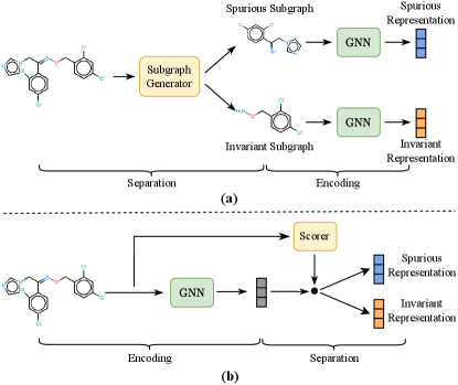
Preliminary studies have made some attempts on molecular graphs chen2022ciga ; yang2022learning ; NEURIPS2022_4d4e0ab9 ; DBLP:conf/kdd/SuiWWL0C22 ; DBLP:conf/iclr/WuWZ0C22 . They explicitly divide graphs to extract invariant substructures, at the granularity of nodes DBLP:conf/kdd/SuiWWL0C22 , edges chen2022ciga ; NEURIPS2022_4d4e0ab9 ; DBLP:conf/kdd/SuiWWL0C22 ; DBLP:conf/iclr/WuWZ0C22 , or motifs yang2022learning . These attempts can be summarized as the “first-separation-then-encoding” paradigm (Figure 1 (a)), which first divides the graph into invariant and spurious parts and then encodes each part separately. We argue that this practice is sub-optimal for extremely complex and entangled graphs, such as real-world molecules jiang2000zinc ; huron1972calculation , since some intricate properties cannot be readily determined by analyzing a subset of the molecular structure jiang2000zinc ; huron1972calculation . Besides, some methods yang2022learning ; NEURIPS2022_4d4e0ab9 require assumptions and inferences about the environmental distribution, which are often untenable for molecules due to the intricate environment. Additionally, the downstream tasks related to molecules are diverse, including regression and classification. However, some methods such as CIGA chen2022ciga and DisC DBLP:journals/corr/abs-2209-14107 can only be applied to single-label classification tasks, due to the constraints imposed by the invariant learning objective function.
To fill these gaps, we present a novel molecule invariant learning framework to effectively capture the invariance of molecular graphs and achieve generalized representation against distribution shifts. In contrast to the conventional approaches, we propose a “first-encoding-then-separation strategy” (Figure 1 (b)). Specifically, we first employ a Graph Neural Network (GNN) DBLP:conf/iclr/KipfW17 ; DBLP:conf/nips/HamiltonYL17 ; DBLP:conf/iclr/XuHLJ19 to encode the molecule (i.e., encoding GNN), followed by a residual vector quantization module to alleviate the over-fitting to training data distributions while preserving the expressivity of the encoder. We then utilize another GNN to score the molecule representation (i.e., scoring GNN), which measures the contributions of each dimension to the target in latent space, resulting in a clear separation between invariant and spurious representations. Finally, we design a self-supervised learning objective chen2020simple ; chen2021exploring ; grill2020bootstrap that aims to encourage the identified invariant features to effectively preserve label-related information while discarding environment-related information. It is deserving of note that the objective is task-agnostic, which means that our method can be applied to various tasks, including regression and single- or multi-label classification.
Our main contributions can be summarized as follows:
-
•
We propose a paradigm of “first-encoding-then-separation” using an encoding GNN and a scoring GNN, which enables us to effectively identify invariant features from highly complex graphs.
-
•
We introduce a residual vector quantization module that strikes a balance between model expressivity and generalization. The quantization acts as the bottleneck to enhance generalization, while the residual connection complements the model’s expressivity.
-
•
We design a self-supervised invariant learning objective that facilitates the precise capture of invariant features. This objective is versatile, task-agnostic, and applicable to a variety of tasks.
-
•
We conduct comprehensive experiments on a diverse set of real-world datasets with various distribution shifts. The experimental results demonstrate the superiority of our method compared to state-of-the-art approaches.
2 Related Work
OOD Generalization and Invariance Principle.
The susceptibility of deep neural networks to substantial performance degradation under distribution shifts has led to a proliferation of research focused on out-of-distribution (OOD) generalization DBLP:journals/corr/abs-2108-13624 . Three lines of methods have been studied for OOD generalization on Euclidean data, including group distributionally robust optimization DBLP:conf/icml/KruegerCJ0BZPC21 ; DBLP:conf/iclr/SagawaKHL20 ; DBLP:conf/icml/ZhangSZFR22 , domain adaptation DBLP:journals/jmlr/GaninUAGLLML16 ; DBLP:conf/eccv/SunS16 ; DBLP:conf/eccv/LiTGLLZT18 and invariant learning DBLP:journals/corr/abs-1907-02893 ; DBLP:conf/nips/AhujaCZGBMR21 ; DBLP:conf/icml/CreagerJZ21 . Group distributionally robust optimization considers groups of distributions and optimize across all groups simultaneously. Domain adaptation aims to align the data distributions but may fail to find an optimal predictor without additional assumptions DBLP:journals/corr/abs-1907-02893 ; DBLP:conf/nips/AhujaCZGBMR21 ; DBLP:conf/icml/0002CZG19 . Invariant learning aims to learn invariant representation satisfying the invariant principle DBLP:conf/nips/AhujaCZGBMR21 ; DBLP:journals/jmlr/Rojas-CarullaST18 , which includes two assumptions: (1) sufficiency, meaning the representation has sufficient predictive abilities, (2) invariance, meaning representation is invariant to environmental changes. However, most methods require environmental labels, which are expensive to obtain for molecules chen2022ciga , and direct application of these methods to complicated non-Euclidean molecular structure does not yield promising results DBLP:journals/corr/abs-2201-09637 ; DBLP:journals/corr/abs-2008-01883 ; chen2022ciga .
OOD Generalization on Graphs.
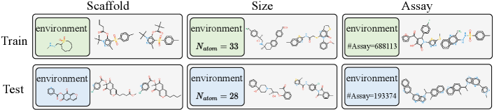
Recently, there has been growing attention on the graph-level representations under distribution shifts from the perspective of invariant learning. Some methods chen2022ciga ; DBLP:journals/corr/abs-2209-14107 ; NEURIPS2022_4d4e0ab9 ; DBLP:conf/kdd/SuiWWL0C22 ; yang2022learning follows the “first-separation-then-encoding” paradigm, and they make attempt to capture the invariant substructures by dividing nodes and edges in the explicit structural space. However, these methods suffer from the difficulty in dividing molecule graphs in raw space due to the complex and entangled molecular structure DBLP:conf/kdd/LiuZXL022 . Moreover, MoleOOD yang2022learning and GIL NEURIPS2022_4d4e0ab9 require inference of unavailable environmental labels, which entails prior assumptions on the environmental distribution. And the objective of invariant learning may hinder the application, e.g., CIGA chen2022ciga and DisC DBLP:journals/corr/abs-2209-14107 can only apply to single-label classification rather than to regression and multi-label tasks. Additionally, OOD-GNN li2022ood does not use the invariance principle. It proposes to learn disentangled graph representations, but requires computing global weights for all data, leading to a high computational cost. OOD generalization on graphs can also be improved by another line of relevant works DBLP:conf/iclr/WuWZ0C22 ; DBLP:conf/icml/MiaoLL22 ; DBLP:conf/kdd/LiuZXL022 on GNN explainability DBLP:conf/nips/YingBYZL19 ; yuan2022explainability , which aims to provide a rationale for prediction. However, they may fail in some distribution shift cases chen2022ciga . And DIR DBLP:conf/iclr/WuWZ0C22 and GSAT DBLP:conf/icml/MiaoLL22 also divide graphs in the raw structural space. Although GREA DBLP:conf/kdd/LiuZXL022 learns in the latent feature space, it only conducts separation on each node while neglecting the different significance of each representation dimensionality. In this work, we focus on the OOD generalization of molecular graphs, against multi-type of distribution shifts, e.g., scaffold, size, and assay, as shown in Figure 2.
Vector Quantization.
Vector Quantization (VQ) DBLP:conf/nips/OordVK17 ; DBLP:conf/nips/RazaviOV19 acts as a bottleneck of representation learning. It discretizes continuous input data in the hidden space by assigning them to the nearest vectors in a predefined codebook. Some studies DBLP:conf/nips/RazaviOV19 ; DBLP:journals/corr/abs-2112-00384 ; DBLP:journals/taslp/ZeghidourLOST22 ; xia2023molebert have demonstrated its effectiveness to enhance model robustness against data corruptions. Other studies DBLP:conf/nips/LiuLKGSMB21 ; DBLP:journals/corr/abs-2207-11240 ; DBLP:journals/corr/abs-2202-01334 find that taking VQ as an inter-component communication within neural networks can contribute to the model generalization ability. However, we posit that while VQ can improve generalization against distribution shifts, it may also limit the model’s expressivity and potentially lead to under-fitting. To address this concern, we propose to equip the conventional VQ with a residual connection to strike a balance between model generalization and expressivity.
3 Preliminaries
3.1 Problem Definition
We focus on the OOD generalization of molecules. Let be the molecule graph space and be the label space, the goal is to find a predictor to map the input into the label . Generally, we are given a set of datasets collected from multiple environments . Each contains pairs of an input molecule and its label: that are drawn from the joint distribution of environment . However, the information of environment is always not available for molecules, thus we redefine the training joint distribution as , and the testing joint distribution as , where . We denote joint distribution across all environment as . Formally, the goal is to learn an optimal predictor based on training data and can generalize well across all distributions:
| (1) |
where is the empirical risk function. Moreover, since the joint distribution can be written as , the OOD problem can be refined into two cases, namely covariate and concept shift moreno2012unifying ; quinonero2008dataset ; widmer1996learning ; DBLP:journals/corr/abs-2206-08452 . In covariate shift, the distribution of input differs. Formally, and . While concept shift occurs when the conditional distribution changes as and . We will consider and distinguish between both cases in our experiments.
3.2 Molecular Representation Learning
We denote a molecule graph by , where is the set of nodes (e.g., atoms) and is the set of edges (e.g., chemical bonds). Generally, the predictor can be denoted as , containing an encoder that extracts representation for each molecule and a downstream classifier that predicts the label with the molecular representation. In particular, the encoder operates in two stages: firstly, by employing a graph neural network DBLP:conf/iclr/KipfW17 ; DBLP:conf/nips/HamiltonYL17 ; DBLP:conf/iclr/XuHLJ19 to generate node representations according to the following equation:
| (2) |
where is the representation of node . Secondly, the encoder utilizes a readout operator to obtain the overall graph representation :
| (3) |
The readout operator can be implemented using a simple, permutation invariant function such as average pooling.
4 Method
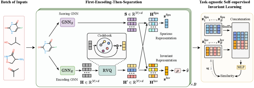
This section presents the details of our proposed method that learns invariant Molecular representation in Latent Discrete space, called iMoLD. Figure 3 shows the overview of iMoLD, which mainly consists of three steps: 1) Using a GNN encoder and a residual vector quantization module to obtain the molecule representation (Section 4.1); 2) Separating the representation into invariant and spurious parts through a GNN scorer (Section 4.2); 3) Optimizing the above process with a task-agnostic self-supervised learning objective (Section 4.3).
4.1 Encoding with Residual Vector Quantization
The current mainstream methods chen2022ciga ; yang2022learning ; DBLP:conf/kdd/SuiWWL0C22 ; NEURIPS2022_4d4e0ab9 ; DBLP:journals/corr/abs-2209-14107 adopt the “first-separation-then-encoding” paradigm, which explicitly divides graphs into invariant and spurious substructures on the granularity of edge, node, or motif, and then encodes each substructure individually. In contrast, we use the opposite paradigm that first encodes the whole molecule followed by separation.
Specifically, given an input molecule , we first use a GNN to encode it, resulting in node representations :
| (4) |
where represents the encoding GNN, is the number of nodes in , and is the dimensionality of features. Inspired by the studies DBLP:conf/nips/LiuLKGSMB21 ; DBLP:journals/corr/abs-2202-01334 that Vector Quantization (VQ) DBLP:conf/nips/OordVK17 ; DBLP:conf/nips/RazaviOV19 is helpful to improve the model generalization on computer vision tasks, we propose a Residual Vector Quantization (RVQ) module to refine the obtained representations.
In the RVQ module, VQ is used to discretize continuous representations into discrete ones. Formally, it introduces a shared learnable codebook as a discrete latent space: , where each . For each node representation in , VQ looks up and fetches the nearest neighbor in the codebook and outputs it as the result. Mathematically,
| (5) |
and denotes the discretization operation which quantizes to in the codebook.
The VQ operation acts as a bottleneck to enhance generalization and alleviate the easy-over-fitting issue caused by distribution shifts. However, it also impairs the expressivity of the model by using a limited discrete codebook to replace the original continuous input, suffering from a potential under-fitting issue. Accordingly, we propose to equip the conventional VQ with a residual connection to strike a balance between model generalization and expressivity. In specific, we incorporate both the continuous and discrete representations to update node representations to :
| (6) |
Similar to VQ-VAE DBLP:conf/nips/OordVK17 ; DBLP:conf/nips/RazaviOV19 , we employ the exponential moving average updates for the codebook:
| (7) |
where is the number of node representations in the -th mini-batch that are quantized to , and is a decay parameter between 0 and 1.
4.2 Separation at Nodes and Features
After encoding, we separate the representation into invariant parts and spurious parts. It is worth noting that our separation is not only performed at the node dimension but also takes into account the feature dimension in the latent space. The reasons are two-fold: 1) Distribution shifts on molecules can occur at both the structure level and the attribute level chen2022ciga , corresponding to the node dimension and the feature dimension in , respectively. 2) The resulting representation may be highly entangled, thus it is advisable to perform a separation on each dimension in the latent space.
Specifically, we use another GNN as a scorer to obtain the separating score :
| (8) |
where represents the scoring GNN, is the number of nodes in , and is the dimensionality of features. denotes the Sigmoid function to constrain each entry in falls into the range of . Then we can capture the invariant and complementary spurious features at both structure and attribute granularity in the latent representation space by applying the separating scores to node representations:
| (9) |
where and denote the invariant and spurious node representations respectively, and is the element-wise product. Finally, the invariant and spurious representation (denoted as and respectively) of can be generated by a readout operator:
| (10) |
4.3 Learning Objective
Our OOD optimization objectives are composed of an invariant learning loss, a task prediction loss, and two additional regularization losses.
Task-agnostic Self-supervised Invariant Learning.
Invariant learning aims to optimize the encoding and the scoring to produce precise invariant and spurious representations. In particular, we need to be invariant under environmental changes. Additionally, we expect the objective to be independent of the downstream task, which allows the method to be not restricted to a specific type of task. To achieve these, we design a task-agnostic and self-supervised invariant learning objective. Specifically, we disturb via concatenating a corresponding in a shuffled batch, resulting in an augmented representation :
| (11) |
where denotes concatenation operator and is batch size.
Inspired by a simple self-supervised learning framework that takes different augmentation views as similar positive pairs and does not require negative samples chen2021exploring , we treat and as positive pairs and push them to be similar, using an MLP-based predictor (denoted as ) that transforms the output of one view and aligns it to the other view. We minimize their negative cosine similarity:
| (12) |
where represents the formula of cosine similarity and denotes stop-gradient operation to prevent collapsing chen2021exploring . We employ as our objective for invariant learning to ensure the invariance of against distribution shifts.
Task Prediction.
The objective of task prediction is to provide an invariant presentation with sufficient predictive abilities. During training, the choice of prediction loss function depends on the type of task. For classification tasks, we employ the cross-entropy loss, while for regression tasks, we use the mean squared error loss. Take the binary classification task as an example, the cross-entropy loss is computed between the predicted and the ground-truth label :
| (13) |
Scoring GNN Regularization.
For the scoring , we apply a penalty to the separation of invariant features, preventing abundance or scarcity and ensuring a reasonable selection. To achieve this, we introduce a regularization term to constrain the size of the selected invariant features:
| (14) |
where denotes a matrix with all entries as 1, is the Frobenius dot product and is a pre-defined threshold between 0 and 1.
Codebook Regularization.
In the RVQ module, following VQ-VAE DBLP:conf/nips/OordVK17 ; DBLP:conf/nips/RazaviOV19 , to encourage to remain close to the selected codebook embedding in Equation (5) and prevent it from frequently fluctuating between different embeddings, we add a commitment loss to foster that commits to and does not grow uncontrollably:
| (15) |
Finally, the learning objective can be defined as the weighted sum of the above losses:
| (16) |
where , and are hyper-parameters to control the weights of (in Equation (12)), (in Equation (14)) and (in Equation (15)), respectively.
5 Experiments
In this section, we conduct extensive experiments to answer the research questions. (RQ1) Can our method iMoLD achieve better OOD generalization performance against SOTA baselines? (RQ2) How does each of the component we propose contribute to the final performance? (RQ3) How can we understand the latent discrete space induced by the proposed RVQ?
| Method | GOOD-HIV | GOOD-ZINC | GOOD-PCBA | |||||||||
|---|---|---|---|---|---|---|---|---|---|---|---|---|
| scaffold | size | scaffold | size | scaffold | size | |||||||
| covariate | concept | covariate | concept | covariate | concept | covariate | concept | covariate | concept | covariate | concept | |
| ERM | 69.55(2.39) | 72.48(1.26) | 59.19(2.29) | 61.91(2.29) | 0.1802(0.0174) | 0.1301(0.0052) | 0.2319(0.0072) | 0.1325(0.0085) | 17.11(0.34) | 21.93(0.74) | 17.75(0.46) | 15.60(0.55) |
| IRM | 70.17(2.78) | 71.78(1.37) | 59.94(1.59) | -(-) | 0.2164(0.0160) | 0.1339(0.0043) | 0.6984(0.2809) | 0.1336(0.0055) | 16.89(0.29) | 22.37(0.43) | 17.68(0.36) | 15.82(0.52) |
| VREx | 69.34(3.54) | 72.21(1.42) | 58.49(2.28) | 61.21(2.00) | 0.1815(0.0154) | 0.1287(0.0053) | 0.2270(0.0136) | 0.1311(0.0067) | 17.10(0.20) | 21.65(0.82) | 17.80(0.35) | 15.85(0.47) |
| GroupDRO | 68.15(2.84) | 71.48(1.27) | 57.75(2.86) | 59.77(1.95) | 0.1870(0.0128) | 0.1323(0.0041) | 0.2377(0.0147) | 0.1333(0.0064) | 16.55(0.39) | 21.91(0.93) | 16.74(0.60) | 15.21(0.66) |
| Coral | 70.69(2.25) | 72.96(1.06) | 59.39(2.90) | 60.29(2.50) | 0.1769(0.0152) | 0.1303(0.0057) | 0.2292(0.0090) | 0.1261(0.0060) | 17.00(0.38) | 22.00(0.46) | 17.83(0.31) | 16.88(0.58) |
| DANN | 69.43(2.42) | 71.70(0.90) | 62.38(2.65) | 65.15(3.13) | 0.1746(0.0084) | 0.1269(0.0042) | 0.2326(0.0140) | 0.1348(0.0091) | 17.20(0.46) | 22.03(0.72) | 17.71(0.26) | 15.78(0.40) |
| Mixup | 70.65(1.86) | 71.89(1.73) | 59.11(3.11) | 62.80(2.43) | 0.2066(0.0123) | 0.1391(0.0071) | 0.2531(0.0150) | 0.1547(0.0082) | 16.52(0.33) | 20.52(0.50) | 17.42(0.29) | 13.71(0.37) |
| DIR | 68.44(2.51) | 71.40(1.48) | 57.67(3.75) | 74.39(1.45) | 0.3682(0.0639) | 0.2543(0.0454) | 0.4578(0.0412) | 0.3146(0.1225) | 16.33(0.39) | 23.82(0.89) | 16.04(1.14) | 16.80(1.17) |
| GSAT | 70.07(1.76) | 72.51(0.97) | 60.73(2.39) | 56.96(1.76) | 0.1418(0.0077) | 0.1066(0.0046) | 0.2101(0.0095) | 0.1038(0.0030) | 16.45(0.17) | 20.18(0.74) | 17.57(0.40) | 13.52(0.90) |
| GREA | 71.98(2.87) | 70.76(1.16) | 60.11(1.07) | 60.96(1.55) | 0.1691(0.0159) | 0.1157(0.0084) | 0.2100(0.0081) | 0.1273(0.0044) | 16.28(0.34) | 20.23(1.53) | 17.12(1.01) | 13.82(1.18) |
| CAL | 69.12(1.10) | 72.49(1.05) | 59.34(2.14) | 56.16(4.73) | / | / | / | / | 15.87(0.69) | 18.62(1.21) | 16.92(0.72) | 13.01(0.65) |
| DisC | 58.85(7.26) | 64.82(6.78) | 49.33(3.84) | 74.11(6.69) | / | / | / | / | / | / | / | / |
| MoleOOD | 69.39(3.43) | 69.08(1.35) | 58.63(1.78) | 55.90(4.93) | 0.2752(0.0288) | 0.1996(0.0136) | 0.3468(0.0366) | 0.2275(0.2183) | 12.90(0.86) | 12.92(1.23) | 12.64(0.55) | 10.30(0.36) |
| CIGA | 69.40(1.97) | 71.65(1.33) | 61.81(1.68) | 73.62(1.33) | / | / | / | / | / | / | / | / |
| iMoLD | 72.93(2.29) | 74.32(1.63) | 62.86(2.58) | 77.43(1.32) | 0.1410(0.0054) | 0.1014(0.0040) | 0.1863(0.0139) | 0.1029(0.0067) | 17.32(0.31) | 22.58(0.67) | 18.02(0.73) | 18.21(1.10) |
5.1 Experimental Setup
Datasets.
We employ two real-world benchmarks for OOD molecular representation learning. Details of datasets are in Appendix A.
-
•
GOOD DBLP:journals/corr/abs-2206-08452 , which is a systematic benchmark tailored specifically for graph OOD problems. We utilize three molecular datasets for the graph prediction task: (1) GOOD-HIV wu2018moleculenet , where the objective is binary classification to predict whether a molecule can inhibit HIV; (2) GOOD-ZINC gomez2018automatic , which is a regression dataset aimed at predicting molecular solubility; and (3) GOOD-PCBA wu2018moleculenet , which includes 128 bioassays and forms 128 binary classification tasks. Each dataset comprises two environment-splitting strategies (scaffold and size), and two shift types (covariate and concept) are applied per splitting outcome, resulting in a total of 12 distinct datasets.
-
•
DrugOOD DBLP:journals/corr/abs-2201-09637 , which is a OOD benchmark for AI-aided drug discovery. This benchmark provides three environment-splitting strategies, including assay, scaffold and size, and applies these three splitting to two measurements (IC50 and EC50). As a result, we obtain 6 datasets, and each dataset contains a binary classification task for drug target binding affinity prediction. A detailed description of each environment-splitting strategy is also in Appendix A.
Baselines.
We thoroughly compare our method against ERM DBLP:journals/tnn/Cherkassky97 and two groups of OOD baselines: (1) general OOD algorithms used for Euclidean data, which include domain adaptation methods such as Coral DBLP:conf/eccv/SunS16 and DANN DBLP:journals/jmlr/GaninUAGLLML16 , group distributionally robust optimization method (GroupDRO DBLP:conf/iclr/SagawaKHL20 ), invariant learning methods such as IRM DBLP:journals/corr/abs-1907-02893 and VREx DBLP:conf/icml/KruegerCJ0BZPC21 and data augmentation method (Mixup DBLP:conf/iclr/ZhangCDL18 ). And (2) graph-specific algorithms, including Graph OOD algorithms such as CAL DBLP:conf/kdd/SuiWWL0C22 , DisC DBLP:journals/corr/abs-2209-14107 , MoleOOD yang2022learning and CIGA chen2022ciga , as well as interpretable graph learning methods such as DIR DBLP:conf/iclr/WuWZ0C22 , GSAT DBLP:conf/icml/MiaoLL22 and GREA DBLP:conf/kdd/LiuZXL022 . Details of baselines and implementation are in Appendix B.
Evaluation.
We report the ROC-AUC score for GOOD-HIV and DrugOOD datasets as the task is binary classification. For GOOD-ZINC, we use the Mean Average Error (MAE) since the task is regression. While for GOOD-PCBA, we use Average Precision (AP) averaged over all tasks as the evaluation metric due to extremely imbalanced classes. We run experiments 10 times with different random seeds, select models based on the validation performance and report the mean and standard deviations on the test set.
| Method | IC50 | EC50 | ||||
|---|---|---|---|---|---|---|
| Assay | Scaffold | Size | Assay | Scaffold | Size | |
| ERM | 71.63(0.76) | 68.79(0.47) | 67.50(0.38) | 67.39(2.90) | 64.98(1.29) | 65.10(0.38) |
| IRM | 71.15(0.57) | 67.22(0.62) | 61.58(0.58) | 67.77(2.71) | 63.86(1.36) | 59.19(0.83) |
| Coral | 71.28(0.91) | 68.36(0.61) | 64.53(0.32) | 72.08(2.80) | 64.83(1.64) | 58.47(0.43) |
| MixUp | 71.49(1.08) | 68.59(0.27) | 67.79(0.39) | 67.81(4.06) | 65.77(1.83) | 65.77(0.60) |
| DIR | 69.84(1.41) | 66.33(0.65) | 62.92(1.89) | 65.81(2.93) | 63.76(3.22) | 61.56(4.23) |
| GSAT | 70.59(0.43) | 66.45(0.50) | 66.70(0.37) | 73.82(2.62) | 64.25(0.63) | 62.65(1.79) |
| GREA | 70.23(1.17) | 67.02(0.28) | 66.59(0.56) | 74.17(1.47) | 64.50(0.78) | 62.81(1.54) |
| CAL | 70.09(1.03) | 65.90(1.04) | 66.42(0.50) | 74.54(4.18) | 65.19(0.87) | 61.21(1.76) |
| DisC | 61.40(2.56) | 62.70(2.11) | 61.43(1.06) | 63.71(5.56) | 60.57(2.27) | 57.38(2.48) |
| MoleOOD | 71.62(0.52) | 68.58(1.14) | 65.62(0.77) | 72.69(1.46) | 65.74(1.47) | 65.51(1.24) |
| CIGA | 71.86(1.37) | 69.14(0.70) | 66.92(0.54) | 69.15(5.79) | 67.32(1.35) | 65.65(0.82) |
| iMoLD | 72.11(0.51) | 68.84(0.58) | 67.92(0.43) | 77.48(1.70) | 67.79(0.88) | 67.09(0.91) |
5.2 Main Results (RQ1)
Table 1 and Table 2 present the empirical results on GOOD and DrugOOD benchmarks, respectively. Our method iMoLD achieves the best performance on 16 of the 18 datasets and ranks second on the other two datasets. Among the compared baselines, the graph-specific OOD methods perform best on only 11 datasets, and some general OOD methods outperform them on another 7 datasets. This suggests that although some advanced graph-specific OOD methods can achieve superior performance on some synthetic datasets (e.g., to predict whether a specific motif is present in a synthetic graph DBLP:conf/iclr/WuWZ0C22 ), they may not perform well on molecules due to the realistic and complex data structures and distribution shifts. In contrast, our method is able to achieve the best performance on most of the datasets, which indicates that the proposed identification of invariant features in the latent space is effective for applying the invariance principle to the molecular structure. We also observe that MoleOOD, a method designed specifically for molecules, does not perform well on GOOD-ZINC and GOOD-PCBA, possibly due to its dependence on inferred environments. Inferring environments may become more challenging for larger-scale datasets, such as GOOD-ZINC and GOOD-PCBA, which contain hundreds of thousands of data and more complex tasks (e.g., PCBA has a total of 128 classification tasks). Our method does not require the inference of environment, and is shown to be effective on datasets of diverse scales and tasks.
5.3 Ablation Studies of Components (RQ2)
We conduct ablation studies to analyze how each proposed component contributes to the final performance. Three groups of variants are included: (1) The first group is to investigate the RVQ module. It consists of ERM and ERM (+RVQ), to explore the performance of the simplest ERM and the role of applying the RVQ to it. It also consists of variants of our method, including w/o VQ, which uses instead of in Equation (9) to obtain and ; w/o R, which obtains and without a residual connection by using the output of discretization in Equation (5). (2) The second group is to investigate the impact of each individual training objective, including w/o , w/o and w/o , which remove , and from the final objective function in Equation (16), respectively. (3) The third group consists of variants that replace our proposed self-supervised invariant learning objective with other methods, including w/ and w/ , which represent the objective functions using CIGA chen2022ciga and GREA DBLP:conf/kdd/LiuZXL022 , respectively.
| GOOD-HIV-Scaffold | GOOD-PCBA-Size | |||
| covariate | concept | covariate | concept | |
| iMoLD | 72.93(2.29) | 74.32(1.63) | 18.02(0.73) | 18.21(1.10) |
| ERM | 69.55(2.39) | 72.48(1.26) | 17.75(0.46) | 15.60(0.55) |
| ERM (+RVQ) | 70.18(1.07) | 73.14(1.99) | 17.84(0.47) | 16.59(0.40) |
| w/o VQ | 70.18(1.60) | 72.88(0.66) | 17.88(1.57) | 17.37(0.82) |
| w/o R | 72.40(2.21) | 73.03(0.15) | 17.37(0.62) | 12.99(2.09) |
| w/o | 70.73(1.35) | 71.89(1.80) | 17.55(0.34) | 17.05(0.87) |
| w/o | 71.47(0.72) | 72.39(0.87) | 17.33(0.68) | 17.91(0.34) |
| w/o | 70.20(4.07) | 71.98(1.36) | 17.24(1.02) | 17.68(2.20) |
| w/ | 71.23(1.31) | 73.31(1.73) | / | / |
| w/ | 72.33(1.23) | 72.94(2.30) | 17.93(0.55) | 16.86(0.50) |
Table 3 reports the results on the scaffold-split of GOOD-HIV and the size-split of GOOD-PCBA. We observe that the addition of the RVQ module can improve performance without using any invariant learning algorithms. This indicates that the designed RVQ is effective. Notably, on the GOOD-HIV dataset, removing the VQ module results in significant performance degradation. While on the GOOD-PCBA dataset, removing the residual connection leads to a significant performance drop. This observation may be attributed to the larger scale and more complex task of the GOOD-PCBA dataset. Although VQ improves the generalization, it reduces the expressivity capacity of the model. Thus, achieving a balance between the benefits and weaknesses brought by VQ is necessary with the proposed RVQ module. By observing the second group, we can conclude that each module is instrumental to the final performance. Removing the invariant learning objective and commitment loss results in more pronounced performance degradation, suggesting that the invariant learning objective is effective and indispensable, as well as the need for a constraint term to justify the output of the encoder and the codebook in VQ. By comparing the third group of results, we find that our proposed learning objective outperforms the existing methods, which shows that our approach can not only be applied to a wider range of tasks but also achieve better performance. Moreover, to investigate the robustness of our model, we perform a hyper-parameter sensitivity analysis in Appendix C.1.
5.4 Analysis of Latent Discrete Space (RQ3)
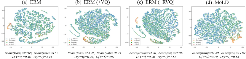
To further explore why our method performs better and to understand the superiority of the introduced discrete latent space, we visualize the projection of extracted on both training and validation set when the model achieves the best score on the validation set, using t-SNE van2008visualizing on the covariate-shift dataset of GOOD-HIV-Scaffold in Figure 4 (d). We also visualize the results of some baselines, including the vanilla ERM (Figure 4 (a)), the ERM equipped with VQ after encoder (ERM(+VQ), Figure 4 (b)), and with the RVQ module (ERM(+RVQ), Figure 4 (c)). We additionally compute the 1-order Wasserstein distance villani2009optimal between the features on the training and validation sets of each class, to quantify the dissimilarity in the feature distribution across varying environments. We find that adding the VQ or RVQ after the encoder results in a more uniform distribution of features and lower feature distances, due to the fact that VQ makes it possible to reuse previously encountered embeddings in new environments by discretizing them. Moreover, the feature distribution of our method is more uniform and the distance is smaller. This suggests that our method is effective in identifying features that are invariant across different environments. Moreover, we also observe that all ERM methods achieve lower validation scores with higher training scores, implying that these methods are prone to overfitting. Our method, on the other hand, achieves not only a higher validation score but also a higher corresponding training score, thereby demonstrating its ability to overcome the problem of easy overfitting and improve the generalization ability effectively.
6 Conclusion
In this work, we propose a new framework that learns invariant molecular representation against distribution shifts. We adopt a “first-encoding-then-separation” strategy, wherein a combination of encoding GNN and residual vector quantization is utilized to derive molecular representation in latent discrete space. Then we learn a scoring GNN to identify invariant features from this representation. Moreover, we design a task-agnostic self-supervised learning objective to enable precise invariance identification and versatile applicability to various tasks. Extensive experiments on real-world datasets demonstrate the superiority of our method on the molecular OOD problem. Overall, our proposed framework presents a promising approach for learning invariant molecular representations and offers valuable insights for addressing distribution shifts in molecular data analysis.
Acknowledgments
This work was supported by the National Key Research and Development Program of China (2022YFB4500300), National Natural Science Foundation of China (NSFCU19B2027, NSFC91846204, NSFC62302433), joint project DH-2022ZY0012 from Donghai Lab, and sponsored by CCF-Tencent Open Fund (CCF-Tencent RAGR20230122). We want to express gratitude to the anonymous reviewers for their hard work and kind comments.
References
- [1] Eugene N Muratov, Jürgen Bajorath, Robert P Sheridan, Igor V Tetko, Dmitry Filimonov, Vladimir Poroikov, Tudor I Oprea, Igor I Baskin, Alexandre Varnek, Adrian Roitberg, et al. Qsar without borders. Chemical Society Reviews, 49(11):3525–3564, 2020.
- [2] Stephani Joy Y Macalino, Vijayakumar Gosu, Sunhye Hong, and Sun Choi. Role of computer-aided drug design in modern drug discovery. Archives of pharmacal research, 38:1686–1701, 2015.
- [3] Justin Gilmer, Samuel S. Schoenholz, Patrick F. Riley, Oriol Vinyals, and George E. Dahl. Neural message passing for quantum chemistry. In ICML, volume 70 of Proceedings of Machine Learning Research, pages 1263–1272. PMLR, 2017.
- [4] Kevin Yang, Kyle Swanson, Wengong Jin, Connor Coley, Philipp Eiden, Hua Gao, Angel Guzman-Perez, Timothy Hopper, Brian Kelley, Miriam Mathea, et al. Analyzing learned molecular representations for property prediction. Journal of chemical information and modeling, 59(8):3370–3388, 2019.
- [5] Yu Rong, Yatao Bian, Tingyang Xu, Weiyang Xie, Ying Wei, Wenbing Huang, and Junzhou Huang. Self-supervised graph transformer on large-scale molecular data. In NeurIPS, 2020.
- [6] Yin Fang, Qiang Zhang, Haihong Yang, Xiang Zhuang, Shumin Deng, Wen Zhang, Ming Qin, Zhuo Chen, Xiaohui Fan, and Huajun Chen. Molecular contrastive learning with chemical element knowledge graph. In AAAI, pages 3968–3976. AAAI Press, 2022.
- [7] Yin Fang, Qiang Zhang, Ningyu Zhang, Zhuo Chen, Xiang Zhuang, Xin Shao, Xiaohui Fan, and Huajun Chen. Knowledge graph-enhanced molecular contrastive learning with functional prompt. Nature Machine Intelligence, pages 1–12, 2023.
- [8] Xiang Zhuang, Qiang Zhang, Bin Wu, Keyan Ding, Yin Fang, and Huajun Chen. Graph sampling-based meta-learning for molecular property prediction. In IJCAI, pages 4729–4737. ijcai.org, 2023.
- [9] John Jumper, Richard Evans, Alexander Pritzel, Tim Green, Michael Figurnov, Olaf Ronneberger, Kathryn Tunyasuvunakool, Russ Bates, Augustin Žídek, Anna Potapenko, et al. Highly accurate protein structure prediction with alphafold. Nature, 596(7873):583–589, 2021.
- [10] Mostafa Karimi, Di Wu, Zhangyang Wang, and Yang Shen. Deepaffinity: interpretable deep learning of compound–protein affinity through unified recurrent and convolutional neural networks. Bioinformatics, 35(18):3329–3338, 2019.
- [11] Deisy Morselli Gysi, Ítalo Do Valle, Marinka Zitnik, Asher Ameli, Xiao Gan, Onur Varol, Susan Dina Ghiassian, JJ Patten, Robert A Davey, Joseph Loscalzo, et al. Network medicine framework for identifying drug-repurposing opportunities for covid-19. Proceedings of the National Academy of Sciences, 118(19):e2025581118, 2021.
- [12] Connor W Coley, Luke Rogers, William H Green, and Klavs F Jensen. Computer-assisted retrosynthesis based on molecular similarity. ACS central science, 3(12):1237–1245, 2017.
- [13] Yuanfeng Ji, Lu Zhang, Jiaxiang Wu, Bingzhe Wu, Long-Kai Huang, Tingyang Xu, Yu Rong, Lanqing Li, Jie Ren, Ding Xue, Houtim Lai, Shaoyong Xu, Jing Feng, Wei Liu, Ping Luo, Shuigeng Zhou, Junzhou Huang, Peilin Zhao, and Yatao Bian. Drugood: Out-of-distribution (OOD) dataset curator and benchmark for ai-aided drug discovery - A focus on affinity prediction problems with noise annotations. CoRR, abs/2201.09637, 2022.
- [14] David Mendez, Anna Gaulton, A Patrícia Bento, Jon Chambers, Marleen De Veij, Eloy Félix, María Paula Magariños, Juan F Mosquera, Prudence Mutowo, Michał Nowotka, et al. Chembl: towards direct deposition of bioassay data. Nucleic acids research, 47(D1):D930–D940, 2019.
- [15] Douglas B Kitchen, Hélène Decornez, John R Furr, and Jürgen Bajorath. Docking and scoring in virtual screening for drug discovery: methods and applications. Nature reviews Drug discovery, 3(11):935–949, 2004.
- [16] Zhenqin Wu, Bharath Ramsundar, Evan N Feinberg, Joseph Gomes, Caleb Geniesse, Aneesh S Pappu, Karl Leswing, and Vijay Pande. Moleculenet: a benchmark for molecular machine learning. Chemical science, 9(2):513–530, 2018.
- [17] Yishay Mansour, Mehryar Mohri, and Afshin Rostamizadeh. Domain adaptation: Learning bounds and algorithms. In COLT, 2009.
- [18] Krikamol Muandet, David Balduzzi, and Bernhard Schölkopf. Domain generalization via invariant feature representation. In ICML (1), volume 28 of JMLR Workshop and Conference Proceedings, pages 10–18. JMLR.org, 2013.
- [19] Martín Arjovsky, Léon Bottou, Ishaan Gulrajani, and David Lopez-Paz. Invariant risk minimization. CoRR, abs/1907.02893, 2019.
- [20] Kartik Ahuja, Ethan Caballero, Dinghuai Zhang, Jean-Christophe Gagnon-Audet, Yoshua Bengio, Ioannis Mitliagkas, and Irina Rish. Invariance principle meets information bottleneck for out-of-distribution generalization. In NeurIPS, pages 3438–3450, 2021.
- [21] Elliot Creager, Jörn-Henrik Jacobsen, and Richard S. Zemel. Environment inference for invariant learning. In ICML, volume 139 of Proceedings of Machine Learning Research, pages 2189–2200. PMLR, 2021.
- [22] Masanori Koyama and Shoichiro Yamaguchi. Out-of-distribution generalization with maximal invariant predictor. CoRR, abs/2008.01883, 2020.
- [23] Jonas Peters, Peter Bühlmann, and Nicolai Meinshausen. Causal inference by using invariant prediction: identification and confidence intervals. Journal of the Royal Statistical Society. Series B (Statistical Methodology), pages 947–1012, 2016.
- [24] Mateo Rojas-Carulla, Bernhard Schölkopf, Richard E. Turner, and Jonas Peters. Invariant models for causal transfer learning. J. Mach. Learn. Res., 19:36:1–36:34, 2018.
- [25] Nianzu Yang, Kaipeng Zeng, Qitian Wu, Xiaosong Jia, and Junchi Yan. Learning substructure invariance for out-of-distribution molecular representations. In Advances in Neural Information Processing Systems (NeurIPS), 2022.
- [26] Yongqiang Chen, Yonggang Zhang, Yatao Bian, Han Yang, Kaili Ma, Binghui Xie, Tongliang Liu, Bo Han, and James Cheng. Learning causally invariant representations for out-of-distribution generalization on graphs. In Advances in Neural Information Processing Systems, 2022.
- [27] Haoyang Li, Ziwei Zhang, Xin Wang, and Wenwu Zhu. Learning invariant graph representations for out-of-distribution generalization. In S. Koyejo, S. Mohamed, A. Agarwal, D. Belgrave, K. Cho, and A. Oh, editors, Advances in Neural Information Processing Systems, volume 35, pages 11828–11841. Curran Associates, Inc., 2022.
- [28] Yongduo Sui, Xiang Wang, Jiancan Wu, Min Lin, Xiangnan He, and Tat-Seng Chua. Causal attention for interpretable and generalizable graph classification. In KDD, pages 1696–1705. ACM, 2022.
- [29] Yingxin Wu, Xiang Wang, An Zhang, Xiangnan He, and Tat-Seng Chua. Discovering invariant rationales for graph neural networks. In ICLR. OpenReview.net, 2022.
- [30] Li-Juan Jiang, Milan Vašák, Bert L Vallee, and Wolfgang Maret. Zinc transfer potentials of the -and -clusters of metallothionein are affected by domain interactions in the whole molecule. Proceedings of the National Academy of Sciences, 97(6):2503–2508, 2000.
- [31] Marie Jose Huron and Pierre Claverie. Calculation of the interaction energy of one molecule with its whole surrounding. i. method and application to pure nonpolar compounds. The Journal of Physical Chemistry, 76(15):2123–2133, 1972.
- [32] Shaohua Fan, Xiao Wang, Yanhu Mo, Chuan Shi, and Jian Tang. Debiasing graph neural networks via learning disentangled causal substructure. CoRR, abs/2209.14107, 2022.
- [33] Thomas N. Kipf and Max Welling. Semi-supervised classification with graph convolutional networks. In ICLR (Poster). OpenReview.net, 2017.
- [34] William L. Hamilton, Zhitao Ying, and Jure Leskovec. Inductive representation learning on large graphs. In NIPS, pages 1024–1034, 2017.
- [35] Keyulu Xu, Weihua Hu, Jure Leskovec, and Stefanie Jegelka. How powerful are graph neural networks? In ICLR. OpenReview.net, 2019.
- [36] Ting Chen, Simon Kornblith, Mohammad Norouzi, and Geoffrey Hinton. A simple framework for contrastive learning of visual representations. In International conference on machine learning, pages 1597–1607. PMLR, 2020.
- [37] Xinlei Chen and Kaiming He. Exploring simple siamese representation learning. In Proceedings of the IEEE/CVF conference on computer vision and pattern recognition, pages 15750–15758, 2021.
- [38] Jean-Bastien Grill, Florian Strub, Florent Altché, Corentin Tallec, Pierre Richemond, Elena Buchatskaya, Carl Doersch, Bernardo Avila Pires, Zhaohan Guo, Mohammad Gheshlaghi Azar, et al. Bootstrap your own latent-a new approach to self-supervised learning. Advances in neural information processing systems, 33:21271–21284, 2020.
- [39] Zheyan Shen, Jiashuo Liu, Yue He, Xingxuan Zhang, Renzhe Xu, Han Yu, and Peng Cui. Towards out-of-distribution generalization: A survey. CoRR, abs/2108.13624, 2021.
- [40] David Krueger, Ethan Caballero, Jörn-Henrik Jacobsen, Amy Zhang, Jonathan Binas, Dinghuai Zhang, Rémi Le Priol, and Aaron C. Courville. Out-of-distribution generalization via risk extrapolation (rex). In ICML, volume 139 of Proceedings of Machine Learning Research, pages 5815–5826. PMLR, 2021.
- [41] Shiori Sagawa, Pang Wei Koh, Tatsunori B. Hashimoto, and Percy Liang. Distributionally robust neural networks. In ICLR. OpenReview.net, 2020.
- [42] Michael Zhang, Nimit Sharad Sohoni, Hongyang R. Zhang, Chelsea Finn, and Christopher Ré. Correct-n-contrast: a contrastive approach for improving robustness to spurious correlations. In ICML, volume 162 of Proceedings of Machine Learning Research, pages 26484–26516. PMLR, 2022.
- [43] Yaroslav Ganin, Evgeniya Ustinova, Hana Ajakan, Pascal Germain, Hugo Larochelle, François Laviolette, Mario Marchand, and Victor S. Lempitsky. Domain-adversarial training of neural networks. J. Mach. Learn. Res., 17:59:1–59:35, 2016.
- [44] Baochen Sun and Kate Saenko. Deep CORAL: correlation alignment for deep domain adaptation. In ECCV Workshops (3), volume 9915 of Lecture Notes in Computer Science, pages 443–450, 2016.
- [45] Ya Li, Xinmei Tian, Mingming Gong, Yajing Liu, Tongliang Liu, Kun Zhang, and Dacheng Tao. Deep domain generalization via conditional invariant adversarial networks. In ECCV (15), volume 11219 of Lecture Notes in Computer Science, pages 647–663. Springer, 2018.
- [46] Han Zhao, Remi Tachet des Combes, Kun Zhang, and Geoffrey J. Gordon. On learning invariant representations for domain adaptation. In ICML, volume 97 of Proceedings of Machine Learning Research, pages 7523–7532. PMLR, 2019.
- [47] Gang Liu, Tong Zhao, Jiaxin Xu, Tengfei Luo, and Meng Jiang. Graph rationalization with environment-based augmentations. In KDD, pages 1069–1078. ACM, 2022.
- [48] Haoyang Li, Xin Wang, Ziwei Zhang, and Wenwu Zhu. Ood-gnn: Out-of-distribution generalized graph neural network. IEEE Transactions on Knowledge and Data Engineering, 2022.
- [49] Siqi Miao, Mia Liu, and Pan Li. Interpretable and generalizable graph learning via stochastic attention mechanism. In ICML, volume 162 of Proceedings of Machine Learning Research, pages 15524–15543. PMLR, 2022.
- [50] Zhitao Ying, Dylan Bourgeois, Jiaxuan You, Marinka Zitnik, and Jure Leskovec. Gnnexplainer: Generating explanations for graph neural networks. In NeurIPS, pages 9240–9251, 2019.
- [51] Hao Yuan, Haiyang Yu, Shurui Gui, and Shuiwang Ji. Explainability in graph neural networks: A taxonomic survey. IEEE Transactions on Pattern Analysis and Machine Intelligence, 2022.
- [52] Aäron van den Oord, Oriol Vinyals, and Koray Kavukcuoglu. Neural discrete representation learning. In NIPS, pages 6306–6315, 2017.
- [53] Ali Razavi, Aäron van den Oord, and Oriol Vinyals. Generating diverse high-fidelity images with VQ-VAE-2. In NeurIPS, pages 14837–14847, 2019.
- [54] Woncheol Shin, Gyubok Lee, Jiyoung Lee, Joonseok Lee, and Edward Choi. Translation-equivariant image quantizer for bi-directional image-text generation. CoRR, abs/2112.00384, 2021.
- [55] Neil Zeghidour, Alejandro Luebs, Ahmed Omran, Jan Skoglund, and Marco Tagliasacchi. Soundstream: An end-to-end neural audio codec. IEEE ACM Trans. Audio Speech Lang. Process., 30:495–507, 2022.
- [56] Jun Xia, Chengshuai Zhao, Bozhen Hu, Zhangyang Gao, Cheng Tan, Yue Liu, Siyuan Li, and Stan Z. Li. Mole-BERT: Rethinking pre-training graph neural networks for molecules. In The Eleventh International Conference on Learning Representations, 2023.
- [57] Dianbo Liu, Alex Lamb, Kenji Kawaguchi, Anirudh Goyal, Chen Sun, Michael C. Mozer, and Yoshua Bengio. Discrete-valued neural communication. In NeurIPS, pages 2109–2121, 2021.
- [58] Frederik Träuble, Anirudh Goyal, Nasim Rahaman, Michael Mozer, Kenji Kawaguchi, Yoshua Bengio, and Bernhard Schölkopf. Discrete key-value bottleneck. CoRR, abs/2207.11240, 2022.
- [59] Dianbo Liu, Alex Lamb, Xu Ji, Pascal Notsawo, Michael Mozer, Yoshua Bengio, and Kenji Kawaguchi. Adaptive discrete communication bottlenecks with dynamic vector quantization. CoRR, abs/2202.01334, 2022.
- [60] Jose G Moreno-Torres, Troy Raeder, Rocío Alaiz-Rodríguez, Nitesh V Chawla, and Francisco Herrera. A unifying view on dataset shift in classification. Pattern recognition, 45(1):521–530, 2012.
- [61] Joaquin Quinonero-Candela, Masashi Sugiyama, Anton Schwaighofer, and Neil D Lawrence. Dataset shift in machine learning. Mit Press, 2008.
- [62] Gerhard Widmer and Miroslav Kubat. Learning in the presence of concept drift and hidden contexts. Machine learning, 23:69–101, 1996.
- [63] Shurui Gui, Xiner Li, Limei Wang, and Shuiwang Ji. GOOD: A graph out-of-distribution benchmark. CoRR, abs/2206.08452, 2022.
- [64] Rafael Gómez-Bombarelli, Jennifer N Wei, David Duvenaud, José Miguel Hernández-Lobato, Benjamín Sánchez-Lengeling, Dennis Sheberla, Jorge Aguilera-Iparraguirre, Timothy D Hirzel, Ryan P Adams, and Alán Aspuru-Guzik. Automatic chemical design using a data-driven continuous representation of molecules. ACS central science, 4(2):268–276, 2018.
- [65] Vladimir Cherkassky. The nature of statistical learning theory. IEEE Trans. Neural Networks, 8(6):1564, 1997.
- [66] Hongyi Zhang, Moustapha Cissé, Yann N. Dauphin, and David Lopez-Paz. mixup: Beyond empirical risk minimization. In ICLR (Poster). OpenReview.net, 2018.
- [67] Laurens Van der Maaten and Geoffrey Hinton. Visualizing data using t-sne. Journal of machine learning research, 9(11), 2008.
- [68] Cédric Villani et al. Optimal transport: old and new, volume 338. Springer, 2009.
- [69] Adam Paszke, Sam Gross, Francisco Massa, Adam Lerer, James Bradbury, Gregory Chanan, Trevor Killeen, Zeming Lin, Natalia Gimelshein, Luca Antiga, Alban Desmaison, Andreas Köpf, Edward Z. Yang, Zachary DeVito, Martin Raison, Alykhan Tejani, Sasank Chilamkurthy, Benoit Steiner, Lu Fang, Junjie Bai, and Soumith Chintala. Pytorch: An imperative style, high-performance deep learning library. In NeurIPS, pages 8024–8035, 2019.
- [70] Matthias Fey and Jan Eric Lenssen. Fast graph representation learning with pytorch geometric. CoRR, abs/1903.02428, 2019.
Appendix A Details of Datasets
A.1 Dataset
In this paper, we use 18 publicly benchmark datasets, 12 of which are from GOOD DBLP:journals/corr/abs-2206-08452 benchmark. They are the combination of 3 datasets (GOOD-HIV, GOOD-ZINC and GOOD-PCBA), 2 types of distribution shift (covariate and concept), and 2 environment-splitting strategies (scaffold and size). The rest 6 datasets are from DrugOOD DBLP:journals/corr/abs-2201-09637 benchmark, including IC50-Assay, IC50-Scaffold, IC50-Size, EC50-Assay, EC50-Scaffold, and EC50-Size. The prefix denotes the measurement and the suffix denotes the environment-splitting strategies. This benchmark exclusively focuses on covariate shift. We use the latest data released on the official webpage111https://drugood.github.io/ based on the ChEMBL 30 database222http://ftp.ebi.ac.uk/pub/databases/chembl/ChEMBLdb/releases/chembl_30. We use the default dataset split proposed in each benchmark. For covariate shift, the training, validation and testing sets are obtained based on environments without interactions. For concept shift, a screening approach is leveraged to scan and select molecules in the dataset. Statistics of each dataset are in Table 4.
| Dataset | Task | Metric | #Train | #Val | #Test | #Tasks | |||
|---|---|---|---|---|---|---|---|---|---|
| GOOD | HIV | scaffold | covariate | Binary Classification | ROC-AUC | 24682 | 4133 | 4108 | 1 |
| concept | Binary Classification | ROC-AUC | 15209 | 9365 | 10037 | 1 | |||
| size | covariate | Binary Classification | ROC-AUC | 26169 | 4112 | 3961 | 1 | ||
| concept | Binary Classification | ROC-AUC | 14454 | 3096 | 10525 | 1 | |||
| ZINC | scaffold | covariate | Regression | MAE | 149674 | 24945 | 24946 | 1 | |
| concept | Regression | MAE | 101867 | 43539 | 60393 | 1 | |||
| size | covariate | Regression | MAE | 161893 | 24945 | 17042 | 1 | ||
| concept | Regression | MAE | 89418 | 19161 | 70306 | 1 | |||
| PCBA | scaffold | covariate | Multi-task Binary Classification | AP | 262764 | 44019 | 43562 | 128 | |
| concept | Multi-task Binary Classification | AP | 159158 | 90740 | 119821 | 128 | |||
| size | covariate | Multi-task Binary Classification | AP | 269990 | 43792 | 31925 | 128 | ||
| concept | Multi-task Binary Classification | AP | 150121 | 32168 | 115205 | 128 | |||
| DrugOOD | IC50 | assay | Binary Classification | ROC-AUC | 34953 | 19475 | 19463 | 1 | |
| scaffold | Binary Classification | ROC-AUC | 22025 | 19478 | 19480 | 1 | |||
| size | Binary Classification | ROC-AUC | 37497 | 17987 | 16761 | 1 | |||
| EC50 | assay | Binary Classification | ROC-AUC | 4978 | 2761 | 2725 | 1 | ||
| scaffold | Binary Classification | ROC-AUC | 2743 | 2723 | 2762 | 1 | |||
| size | Binary Classification | ROC-AUC | 5189 | 2495 | 2505 | 1 | |||
A.2 The Cause of Molecular Distribution Shift
The molecule data can be divided according to different environments, and distribution shifts occur when the source environments of data are different during training and testing. In this work, we investigate three types of environment-splitting strategies, i.e., scaffold, size and assay. And the explanation of each environment are in Table 5.
| Environment | Explanation |
|---|---|
| Scaffold | Molecular scaffold is the fundamental structure of a molecule with desirable bioactive properties. Molecules with the same scaffold belong to the same environment. Distribution shift arises when there is a change in the molecular scaffold. |
| Size | The size of a molecule refers to the total number of atoms in the molecule. Molecular size is also an inherent structural characteristic of molecular graphs. The distribution shift occurs when size changes. |
| Assay | Assay is an experimental method as an examination or determination for molecular characteristics. Due to variations in assay environments and targets, activity values measured by different assays often differ significantly. Samples tested within the same assay belong to a single environment, while a change in the assay leads to a distribution shift. |
Appendix B Details of Implementation
B.1 Baselines
We adopt the following methods as baselines for comparison, one group of which are common approaches for non-Euclidean data:
-
•
ERM DBLP:journals/tnn/Cherkassky97 minimizes the empirical loss on the training set.
-
•
IRM DBLP:journals/corr/abs-1907-02893 seeks to find data representations across all environments by penalizing feature distributions that have different optimal classifiers.
-
•
VREx DBLP:conf/icml/KruegerCJ0BZPC21 reduces the risk variances of training environments to achieve both covariate robustness and invariant prediction.
-
•
GroupDRO DBLP:conf/iclr/SagawaKHL20 minimizes the loss on the worst-performing group, subject to a constraint that ensures the loss on each group remains close.
-
•
Coral DBLP:conf/eccv/SunS16 encourages feature distributions consistent by penalizing differences in the means and covariances of feature distributions for each domain.
-
•
DANN DBLP:journals/jmlr/GaninUAGLLML16 encourages features from different environments indistinguishable by adversarially training a regular classifier and a domain classifier.
-
•
Mixup DBLP:conf/iclr/ZhangCDL18 augments data in training through data interpolation.
And the others are graph-specific methods:
-
•
DIR333https://github.com/Wuyxin/DIR-GNN DBLP:conf/iclr/WuWZ0C22 discovers the subset of a graph as invariant rationale by conducting interventional data augmentation to create multiple distributions.
-
•
GSAT444https://github.com/Graph-COM/GSAT DBLP:conf/icml/MiaoLL22 proposes to build an interpretable graph learning method through the attention mechanism and inject stochasticity into the attention to select label-relevant subgraphs.
-
•
GREA555https://github.com/liugangcode/GREA DBLP:conf/kdd/LiuZXL022 identifies subgraph structures called rationales by environment replacement to create virtual data points to improve generalizability and interpretability.
-
•
CAL666https://github.com/yongduosui/CAL DBLP:conf/kdd/SuiWWL0C22 proposes a causal attention learning strategy for graph classification to encourage GNNs to exploit causal features while ignoring the shortcut paths.
-
•
DisC777https://github.com/googlebaba/DisC DBLP:journals/corr/abs-2209-14107 analyzes the generalization problem of GNNs in a causal view and proposes a disentangling framework for graphs to learn causal and bias substructure.
-
•
MoleOOD888https://github.com/yangnianzu0515/MoleOOD yang2022learning investigates the OOD problem on molecules and designs an environment inference model and a substructure attention model to learn environment-invariant molecular substructures.
-
•
CIGA999https://github.com/LFhase/CIGA chen2022ciga proposes an information-theoretic objective to extract the desired invariant subgraphs from the lens of causality.
B.2 Implementation
Experiments are conducted on one 24GB NVIDIA RTX 3090 GPU.
Baselines.
For datasets in the GOOD benchmark, we use the results provided in the official leaderboard101010https://good.readthedocs.io/en/latest/leaderboard.html. For datasets in the DrugOOD benchmark, we use the official benchmark code111111https://github.com/tencent-ailab/DrugOOD to get the results for ERM, IRM, Coral, and Mixup on the latest version of datasets. The results for GroupDRO and DANN are not reported due to an error occurred while the code was running. For some baselines that do not have reported results, we implement them using public codes. All of the baselines are implemented using the GIN-Virtual DBLP:conf/icml/GilmerSRVD17 ; DBLP:conf/iclr/XuHLJ19 (on GOOD) or GIN DBLP:conf/iclr/XuHLJ19 (on DrugOOD) as the GNN backbone that is parameterized according to the guidance of the respective benchmark. And we conduct a grid search to select hyper-parameters for all implemented baselines.
Our method.
We implement the proposed iMoLD in Pytorch DBLP:conf/nips/PaszkeGMLBCKLGA19 and PyG DBLP:journals/corr/abs-1903-02428 . For all the datasets, we select hyper-parameters by ranging the code book size from , threshold from , from , from , from , and batch size from . For datasets in DrugOOD, we also select dropout rate from . The maximum number of epochs is set to and the learning rate is set to . Please refer to Table 6 for a detailed hyper-parameter configuration of various datasets. The hyper-parameter sensitivity analysis is in Appendix C.1.
| batch-size | dropout | |||||||||
|---|---|---|---|---|---|---|---|---|---|---|
| GOOD | HIV | scaffold | covariate | 0.8 | 4000 | 128 | 0.01 | 0.5 | 0.1 | - |
| concept | 0.7 | 4000 | 256 | 0.01 | 0.5 | 0.1 | - | |||
| size | covariate | 0.7 | 4000 | 256 | 0.01 | 0.5 | 0.1 | - | ||
| concept | 0.9 | 4000 | 1024 | 0.01 | 0.5 | 0.1 | - | |||
| ZINC | scaffold | covariate | 0.3 | 4000 | 32 | 0.01 | 0.5 | 0.1 | - | |
| concept | 0.5 | 4000 | 256 | 0.01 | 0.5 | 0.1 | - | |||
| size | covariate | 0.3 | 4000 | 256 | 0.01 | 0.5 | 0.1 | - | ||
| concept | 0.3 | 4000 | 64 | 0.0001 | 0.5 | 0.1 | - | |||
| PCBA | scaffold | covariate | 0.9 | 10000 | 32 | 0.0001 | 1 | 0.1 | - | |
| concept | 0.9 | 10000 | 32 | 0.0001 | 1 | 0.1 | - | |||
| size | covariate | 0.9 | 10000 | 32 | 0.0001 | 1 | 0.1 | - | ||
| concept | 0.9 | 10000 | 32 | 0.0001 | 1 | 0.1 | - | |||
| DrugOOD | IC50 | assay | 0.7 | 1000 | 128 | 0.001 | 0.5 | 0.1 | 0.5 | |
| scaffold | 0.9 | 1000 | 128 | 0.0001 | 0.5 | 0.1 | 0.5 | |||
| size | 0.7 | 1000 | 128 | 0.01 | 0.5 | 0.1 | 0.1 | |||
| EC50 | assay | 0.7 | 500 | 128 | 0.01 | 0.5 | 0.1 | 0.5 | ||
| scaffold | 0.3 | 500 | 128 | 0.001 | 0.5 | 0.1 | 0.3 | |||
| size | 0.7 | 500 | 128 | 0.001 | 0.5 | 0.1 | 0.1 | |||
Appendix C Additional Experimental Results
C.1 Hyper-parameter Sensitivity Analysis
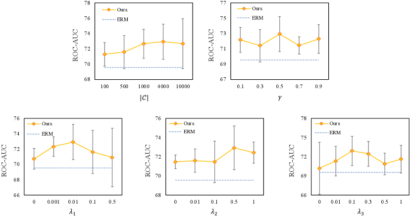
Take the dataset of covariate-shift split of GOODHIV-Scaffold as an example, we conduct extensive experiments to investigate the hyper-parameter sensitivity, and the results are shown in Figure 5. We observe that the performance tends to improve first and then decrease slightly as the size of the codebook increases. This is because a small codebook limits the expressivity of the model, while too large one cuts the advantage of the discrete space. The effect of the threshold is insignificant and there is no remarkable trend. As the , and increase, the performance shows a tendency to increase first and then decrease, indicating that , and are effective and can improve performance within a reasonable range. We also observe that the standard deviation of performance increases as increases, which may be due to the fact that too much weight on the self-supervised invariant learning objective may enhance or affect the performance. The standard deviation is the smallest when , suggesting that neural networks may have more stable outcomes by learning adaptively when there are no constraints, but it is difficult to obtain higher performance. While the standard deviation is the largest when , indicating that the commitment loss in VQ can increase the performance stability.