Learning Performance-oriented Control Barrier Functions Under Complex Safety Constraints and Limited Actuation
Abstract
Control Barrier Functions (CBFs) provide an elegant framework for constraining nonlinear control system dynamics to remain within an invariant subset of a designated safe set. However, identifying a CBF that balances performance—by maximizing the control invariant set—and accommodates complex safety constraints, especially in systems with high relative degree and actuation limits, poses a significant challenge. In this work, we introduce a novel self-supervised learning framework to comprehensively address these challenges. Our method begins with a Boolean composition of multiple state constraints that define the safe set. We first construct a smooth function whose zero superlevel set forms an inner approximation of this safe set. This function is then combined with a smooth neural network to parameterize the CBF candidate. To train the CBF and maximize the volume of the resulting control invariant set, we design a physics-informed loss function based on a Hamilton-Jacobi Partial Differential Equation (PDE). We validate the efficacy of our approach on a 2D double integrator (DI) system and a 7D fixed-wing aircraft system (F16).
1 Introduction
CBFs are a powerful tool to enforce safety constraints for nonlinear control systems [1], with many successful applications in autonomous driving [2], UAV navigation [3], robot locomotion [4], and safe reinforcement learning [5]. For control-affine nonlinear systems, CBFs can be used to construct a convex quadratic programming (QP)-based safety filter deployed online to safeguard against potentially unsafe control commands. The induced safety filter, denoted as CBF-QP, corrects the reference controller to remain in a safe control invariant set.
While Control Barrier Functions (CBFs) provide an efficient method to ensure safety, finding such functions can be challenging. Specifically, there is no guarantee that the resulting safety filter will remain feasible throughout operation. This is primarily because the “model-free” construction of the filter only incorporates the constraints. Complex constraints, high relative degree, and bounded actuation exacerbate the challenge of ensuring feasibility. Various techniques have been proposed to address these challenges such as CBF composition for complex constraints [6, 7, 8, 9], higher-order CBFs for high relative degree [10] [11], and integral CBFs [12] for limited actuation. Despite significant progress, these approaches can make the filter overly restrictive, thus limiting performance.
Contributions
We propose a novel self-supervised learning framework for CBF synthesis that systematically addresses all the above challenges. First, we handle complex safety constraints and high relative degree in CBF synthesis by encoding the safety constraints into the CBF parameterization with minimal conservatism. Second, we design a physics-informed training loss function based on Hamilton-Jacobi (HJ) reachability analysis [13] to satisfy bounded actuation while maximizing the learned control invariant set volume. We evaluate our method on the double-integrator and the high-dimensional fixed-wing aircraft system and demonstrate that the proposed method effectively learns a performant CBF even with complex safety constraints. We call the proposed framework Physics-informed Neural Network (PINN)-CBF [14].
1.1 Related work
Complex safety constraints
For a safe set described by Boolean logical operations on multiple constraints, [6] composes multiple CBFs accordingly through the non-smooth min/max operators.[7] introduces smooth composition of logical operations on constraints, which was later extended to simultaneously handle actuation and state constraints [8][9] using integral CBFs [12]. [15] proposes an algorithmic way to create a single smooth CBF arbitrarily composing both min and max operators. Such smooth bounds have been used in changing environments [16]. Notably, [17] ensures the input constrained feasibility of the CBF condition while composing multiple CBFs.
High-order CBF
High-order CBF (HOCBF) [10] and exponential CBF [11] are systematicly approach CBF construction when the safety constraints have high relative degree. However, controlling the conservatism of these approaches is a challenge. To reduce conservatism or improve the performance of HOCBF, various learning frameworks have been proposed [18, 19, 20] that allow tuning of the class functions used in the CBF condition.
Learning CBF with input constraints
Motivated by the difficulty of hand-designing CBFs, learning-based approaches building on the past [21] have emerged in recent years as an alternative [22, 23, 24, 25]. Liu et al. [26] explicitly consider input constraints in learning a CBF by finding counterexamples on the -level set of the CBF for training, while Dai et al. [27] propose a data-efficient prioritized sampling method. [28] explores adaptive sampling for training HJB NN models favoring sharp gradient regions. Drawing tools from reachability analysis, the recent work [29] iteratively expands the volume of the control invariant set by learning the policy value function and improving the performance through policy iteration. Similarly, Dai et al. [30] expand conservative hand-crafted CBFs by learning on unsafe and safe trajectories, and Qin et al. [31] applies actor-critic RL framework to learn a CBF value function while [32] learns a control policy and CBF together for black-box constraints and dynamics. Our method differs by being controller-independent and basing its learning objective on the HJ partial differential equation (PDE), which defines the maximal control invariant set, without requiring trajectory training data.
HJ reachability-based methods
The value functions in HJ reachability analysis have been extended to construct control barrier-value functions (CBVF) [33] and control Lyapunov-value functions [34], which can be computed using existing toolboxes [35]. Tokens et al. [36] further apply such tools to refine existing CBF candidates, and Bansal et al. [37] learn neural networks solution to a HJ PDE for reachability analysis. Of particular interest to our work is the CBVF, which is close to the CBF formulation and provides a characterization of the viability kernel. Our work aims to learn a neural network CBF from data without using computational tools based on spatial discretization.
Notation
An extended class function is a function for some that is strictly increasing and satisfies . We denote as the -superlevel set of a continuous function . The positive and negative parts of a number are denoted by and , respectively. Let denote the logical operations of conjunction, disjunction, and negation, respectively. For two statements and , we have and .
2 Background and Problem Statement
Consider a continuous time control-affine system:
| (1) |
where is the domain of the system, is the state, is the control input, denotes the control input constraint. We assume that , are locally Lipschitz continuous and is a convex polyhedron. We denote the solution of (1) at time by . Given a set that represents a safe subset of the state space, the general objective of safe control design is to find a control law that renders invariant under the closed-loop dynamics , i.e., if for some , then for all . A general approach to solving this problem is through control barrier functions.
2.1 Control Barrier Functions
Suppose the safe set is defined by the -superlevel set of a smooth function such that . For to be control invariant, the boundary function must satisfy when by Nugomo’s theorem [38]. However, since does not necessarily satisfy the condition, we settle with finding a control invariant set contained in through CBFs.
Definition 1 (Control barrier function).
Let be the -superlevel set of a continuously differentiable function . Then is a control barrier function for system (1) if there exists an extended class function such that
| (2) |
where and are the Lie derivatives of .
Given a CBF , the non-empty set of point-wise safe control actions is given by any locally Lipschitz continuous controller renders the set forward invariant for the closed-loop system, which enables the construction of a minimally-invasive safety filter:
| (3) |
where is any given reference but potentially unsafe controller. Under the assumption that is a polyhedron, is also a polyhedral set and problem (3) becomes a convex QP.
2.2 Problem Statement
While the CBF-QP filter is minimally invasive and guarantees for all time, a small essentially limits the ability of the reference control to execute a task. To take the performance of the reference controller into account, we consider the following problem.
Problem 1 (Performance-Oriented CBF).
Given the input-constrained system (1) and a safe set defined by complex safety constraints (to be specified in Section 3.1), synthesize a CBF with an induced control invariant set such that (i) and (ii) the volume of is maximized. Formally, this problem can be cast as an infinite-dimensional optimization problem:
| (4) | |||||
where is the class of scalar-valued continuously differentiable functions.
3 Proposed Method
In this section, we present our three-step method of learning PINN-CBF :
-
(S1)
Composition of complex state constraints: Given multiple state constraints composed by Boolean logic describing the safe set , we equivalently represent as a zero super level set of a single non-smooth function , i.e., .
-
(S2)
Inner approximation of safe set: Given the constraint function obtained from the previous step, we derive a smooth minorizer of , i.e., for all , s.t. .
-
(S3)
Learning performance-oriented CBF: To approximate the largest control invariant subset of , we design a training loss function based on control barrier-value functions and HJ PDE [33]. We propose a parameterization of the CBF and a sampling strategy exploiting the structure of the PDE.
3.1 Composition of Complex State Constraints
Suppose we are given sets where each is continuously differentiable and the safe set is described by logical operations on . Since all Boolean logical operations can be expressed as the composition of the three fundamental operations conjunction, disjunction, and negation [6, 15], it suffices to only demonstrate the set operations shown below:
-
1.
Conjunction: AND .
-
2.
Disjunction: OR .
-
3.
Negation: NOT (complement of ).
The conjunction and disjunction of two constraints can be exactly expressed as one constraint composed through the and operator, respectively. Furthermore, negating a constraint only requires flipping the sign of . These logical operations enable us to capture complex geometries and logical constraints as illustrated in the following two examples.
Example 1 (Complex geometric sets).
Consider and two rectangular obstacles given by with . The union of the two rectangular obstacles is a nonconvex set. Define the following functions
and let . Then, we have .
Example 2 (Logical constraints).
Consider the three constraints , at least two of which must be satisfied. This specification is equivalent to the constraint , where
In summary, by composing the and operators, we can construct a level-set function such that . Being an exact description of , however, is not smooth. Next, we find a smooth lower bound of that facilitates CBF design.
3.2 Inner Approximation of Safe Set
To find a smooth lower bound for , we utilize its compositional structure. We bound the operators using the log-sum-exponential function as follows [15] ( follows similarly):
| (5) |
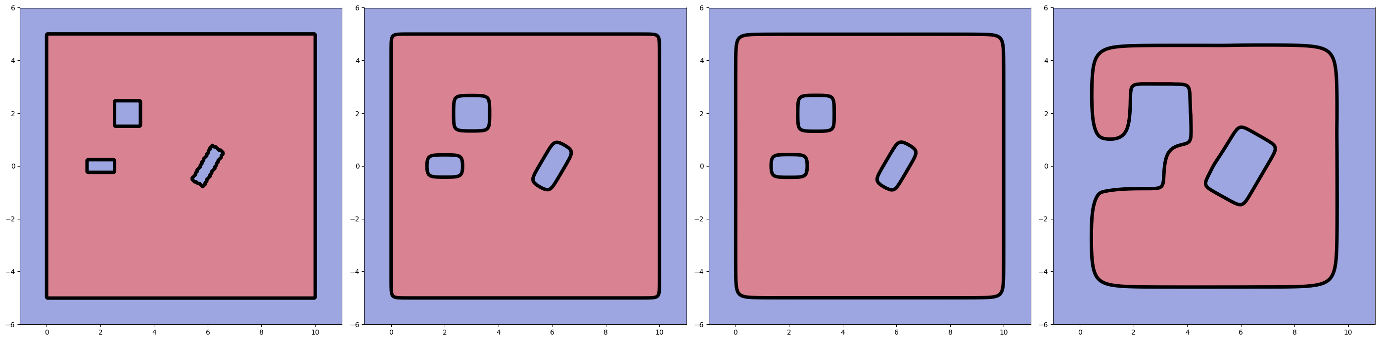
with . As , these bounds can be made arbitrarily accurate. We note that both the lower and upper bounds in (5) are smooth and strictly increasing in each input . Therefore, to obtain a lower bound of , it suffices only to compose the lower bounds on each and function. In Figure 2 we show the effect of on the resulting inner approximation.
3.3 Learning PINN-CBF
The smooth function , whose -superlevel set provides an inner approximation of the safe set , is not necessarily a CBF. Thus, we aim to find the “closest” CBF approximation of . We learn our Neural Network (NN) model using a Hamilton-Jacobi (HJ) PDE from reachability analysis whose infinite-time horizon solution precisely characterizes the CBF maximizing the volume of . Our neural network model is trained by minimizing the PDE residual, grounding the method in physics, and justifying its name (PINN)-CBF.
Hamilton-Jacobi PDE for reachability
Consider the dynamics (1) in the time interval , where and are the initial time and state, respectively. Define as the set of Lebesgue measurable functions . Let denote the unique solution of (1) given and . Given a bounded Lipschitz continuous function , the viability kernel of is defined as
| (6) |
which is the set of all initial states within from which there exists an admissible control signal that keeps the system trajectory within during the time interval . Solving for the viability kernel can be posed as an optimal control problem, where can be expressed as the superlevel set of a value function called control barrier-value function (CBVF).
Definition 2 (CBVF [33]).
Given a discount factor , the control barrier-value function is defined as .
For , we have [33, Proposition 2]. Additionally, is the unique Lipschitz continuous viscosity solution of the following HJ PDE with terminal condition [33, Theorem 3]:
| (7) |
Under mild assumptions of Lipschitz continuous dynamics and being a signed distance function, is differentiable almost everywhere [39]. Furthermore, taking , the steady state solution gives us the maximal control invariant set contained in [33, Section II.B]:
| (8) |
We will leverage the above PDE to learn a CBF whose zero superlevel set approximates the maximal control invariant set.
CBF parameterization In the context of our problem, we are interested in the viability kernel of , where is the smoothed composition of the constraints. Thus, our goal is to learn a CBF that satisfies the PDE . To this end, we parameterize the CBF candidate as
| (9) |
where is a non-negative continuously differentiable function approximator with parameters . In this paper, we parameterize in the form of a multi-layer perceptron:
| (10) |
where are the learnable parameters, is a smooth activation such as the ELU, Tanh, or Swish functions [40], and is a smooth function with non-negative outputs, i.e., . We choose as the Softplus function, .
The parameterization (9) offers several advantages over using a standard MLP model for . First, it accelerates learning by enforcing the non-negativity constraint in (8) by design. Second, complex constraints are directly integrated into the system via , simplifying the learning process. Importantly, is automatically non-positive in regions containing obstacles, allowing the learning process to focus elsewhere.
In summary, the parameterization in (9) ensures that is smooth and satisfies for all , implying that by construction.
Initialization We propose a specialized initialization scheme by letting , initializing the candidate with . This initialization favors finding the closest CBF to during training. Setting only the last layer to zero allows training to break symmetry and retain gradient flow.
Training loss and sampling distribution Given the parameterization (9), we now propose to train to approximately satisfy the steady-state HJ PDE. This leads to the following physics-informed risk minimization
| (11a) | ||||
| (11b) | ||||
| (11c) | ||||
The first loss is the square of the PDE residual to increase the volume of , while the second loss enforces the CBF condition. We note that the latter is implicitly present in the PDE but not enforced by the corresponding loss .
Finally, represents a sampling distribution over , meaning no learning is required within obstacle regions. Efficient sampling in these regions can be achieved using intelligent sampling methods like envelope rejection [41] or the random walk Metropolis-Hastings (RWMH) [42], both of which are well-suited for cluttered environments. Notably, the training process remains self-supervised, as only domain points are collected for learning.
In the following, we demonstrate that jointly enforcing and together with intelligent sampling (IS) improves the performance and safety of the learned PINN-CBF. We note that for polyhedral actuation constraint sets, the supremum over is achieved at one of the vertices, yielding a closed-form expression. We summarize our self-supervised training method in Algorithm 1.
4 Experiments
We demonstrate the efficacy of PINN-CBF on a 2D double integrator system and a 7D fixed-wing aircraft system. Experiments are performed on Google Colab, where the PINN-CBF training is performed on a T4 GPU with 15GB RAM and its validation on a CPU with 52GB RAM. The code is available at https://github.com/o4lc/PINN-CBF.
4.1 Experiment Setup
Double Integrator
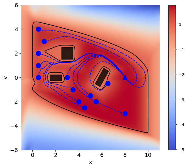
First, we consider the double integrator benchmark , with denoting the position and denoting the velocity. The action represents the acceleration of the system and directly operates on .
We generate a complex obstacle configuration consisting of rotated rectangles and unit walls bordering the state space shown in Fig. 2. Then, we parameterize PINN-CBF following Section 3.3 and train it with uniform samples. At each state in the training data, we compute the values and gradient of using JAX [43] flexible automatic-differentiation and hardware acceleration. The acceleration is bounded by . The nominal controller is given by a PID controller meant to stabilize the system to a target position (see Section A.1).
Fixed-Wing Aircraft The Dubins fixed-wing Plane system has 7D states and 3D limited actuation control. Its full dynamics are shown in Appendix A.2. Sampling and training are done as before except with to compensate for a higher dimensional space . Although , as suggested by naive dimensional scaling, we aim to demonstrate how learning can overcome the curse of dimensionality. The action is bounded in magnitude by . Rectangular obstacles occur in . We chose a nominal trajectory resembling takeoff to evaluate the PINN-CBF filter against relevant baselines on collision avoidance.
4.2 Results
Double-Integrator
We evaluate the combination of loss functions (11b) and (11c) with intelligent sampling (IS) from Algorithm 1, as shown in Table 1. All proposed ablations and baseline methods use the same architecture (9) for a fair comparison, accommodating complex input-space constraints. The MLP for has layer widths of , while DeepReach [37] includes time as an additional input and is applied over the full horizon with .
Using three metrics, We validate at grid samples covering the effective obstacle-free space . The residual error denotes how close the learned CBF is to the maximal-invariant solution of the HJ PDE, measures safety violation, and represents the volume ratio between the learned invariant set and the smoothed safe set, which serves as an upper bound enforced by the architecture.
| Method | Mean over | Mean over | |
|---|---|---|---|
| (IS) | |||
| [22] | |||
| NCBF [26] | |||
| DeepReach [37] |
In the ablations, scalarization with reduces safety violations but decreases volume. In contrast, intelligent sampling lowers residuals and safety violations while increasing volume, suggesting it mitigates the tradeoff of scalarization. Among the baselines, directly enforcing the CBF condition (2) with results in a highly safe but ineffective filter with zero volume. NCBF and DeepReach achieve high volume but with significantly higher safety errors. Next, we will examine how these methods perform on a more complex fixed-wing plane system.
Fixed-Wing Plane The same comparisons conducted for the Double-Integrator are also performed with the following adjustments: all methods utilize a MLP architecture. DeepReach includes an additional input for time. Additionally, validation is carried out on uniformly random sampled states instead of grid samples.
| Model | Mean over | Mean over | Volume of |
|---|---|---|---|
| (IS) | |||
| [22] | |||
| NCBF [26] | |||
| DeepReach [37] |
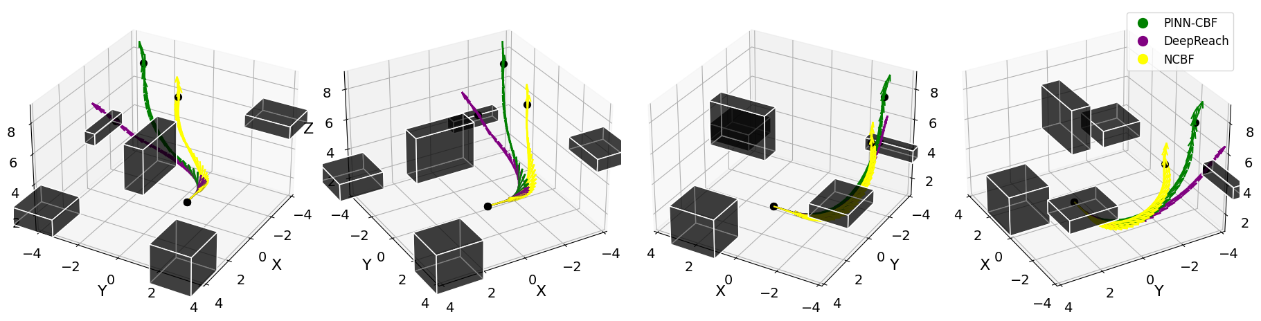
Training with is ineffective, yielding nearly zero volume. The performance of NCBF severely declines due to the increased difficulty of sampling for counterexamples in higher dimensions. In contrast, DeepReach achieves higher volume at the cost of increased safety violations. Our method, PINN-CBF, achieves both low conservatism and safety. To illustrate this, we visualize the performance of PINN-CBF, NCBF, and DeepReach in filtering a nominal trajectory representing takeoff.
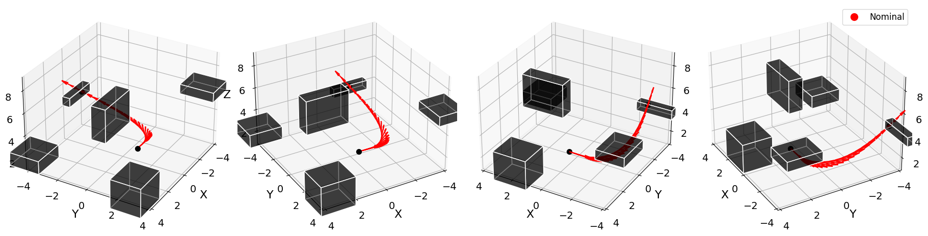
Fixed-Wing Aircraft Example In Fig. 4, the fixed-wing aircraft starting from the given position collides with a 3D obstacle, while in Fig. 4, obstacles are avoided with the PINN-CBF safety filter.
5 Conclusion and Limitations
We introduced a self-supervised framework for learning control barrier functions (CBFs) for limited-actuation systems with complex safety constraints. Our approach maximizes the control invariant set volume through physics-informed learning on a Hamilton-Jacobi (HJ) PDE characterizing the viability kernel. Additionally, we proposed a neural CBF parameterization that leverages the PDE structure.
A key limitation of learning-based CBFs is the lack of guarantees on the control invariant set, as well as the need for many samples, similar to physics-informed methods. Our intelligent sampling (IS) strategy mitigates this to some extent, but the approach remains restricted to specific domains and obstacle configurations. Future work will explore domain-adaptive CBFs that generalize across different obstacle settings, building on recent advances in physics-informed techniques and further investigating links between CBF learning, HJ reachability analysis, and Control Lyapunov Value Functions [44].
References
- Ames et al. [2019] A. D. Ames, S. Coogan, M. Egerstedt, G. Notomista, K. Sreenath, and P. Tabuada. Control barrier functions: Theory and applications. In 2019 18th European control conference (ECC), pages 3420–3431. IEEE, 2019.
- Xiao et al. [2021] W. Xiao, N. Mehdipour, A. Collin, A. Y. Bin-Nun, E. Frazzoli, R. D. Tebbens, and C. Belta. Rule-based optimal control for autonomous driving. In Proceedings of the ACM/IEEE 12th International Conference on Cyber-Physical Systems, pages 143–154, 2021.
- Xu and Sreenath [2018] B. Xu and K. Sreenath. Safe teleoperation of dynamic uavs through control barrier functions. In 2018 IEEE International Conference on Robotics and Automation (ICRA), pages 7848–7855. IEEE, 2018.
- Grandia et al. [2021] R. Grandia, A. J. Taylor, A. D. Ames, and M. Hutter. Multi-layered safety for legged robots via control barrier functions and model predictive control. In 2021 IEEE International Conference on Robotics and Automation (ICRA), pages 8352–8358. IEEE, 2021.
- Marvi and Kiumarsi [2021] Z. Marvi and B. Kiumarsi. Safe reinforcement learning: A control barrier function optimization approach. International Journal of Robust and Nonlinear Control, 31(6):1923–1940, 2021.
- Glotfelter et al. [2017] P. Glotfelter, J. Cortés, and M. Egerstedt. Nonsmooth barrier functions with applications to multi-robot systems. IEEE control systems letters, 1(2):310–315, 2017.
- Lindemann and Dimarogonas [2018] L. Lindemann and D. V. Dimarogonas. Control barrier functions for signal temporal logic tasks. IEEE control systems letters, 3(1):96–101, 2018.
- Rabiee and Hoagg [2023] P. Rabiee and J. B. Hoagg. Soft-minimum barrier functions for safety-critical control subject to actuation constraints. In 2023 American Control Conference (ACC), pages 2646–2651. IEEE, 2023.
- Rabiee and Hoagg [2025] P. Rabiee and J. B. Hoagg. Soft-minimum and soft-maximum barrier functions for safety with actuation constraints. Automatica, 171:111921, 2025.
- Xiao and Belta [2021] W. Xiao and C. Belta. High-order control barrier functions. IEEE Transactions on Automatic Control, 67(7):3655–3662, 2021.
- Nguyen and Sreenath [2016] Q. Nguyen and K. Sreenath. Exponential control barrier functions for enforcing high relative-degree safety-critical constraints. In 2016 American Control Conference (ACC), pages 322–328. IEEE, 2016.
- Ames et al. [2020] A. D. Ames, G. Notomista, Y. Wardi, and M. Egerstedt. Integral control barrier functions for dynamically defined control laws. IEEE control systems letters, 5(3):887–892, 2020.
- Bansal et al. [2017] S. Bansal, M. Chen, S. Herbert, and C. J. Tomlin. Hamilton-jacobi reachability: A brief overview and recent advances. In 2017 IEEE 56th Annual Conference on Decision and Control (CDC), pages 2242–2253. IEEE, 2017.
- Karniadakis et al. [2021] G. E. Karniadakis, I. G. Kevrekidis, L. Lu, P. Perdikaris, S. Wang, and L. Yang. Physics-informed machine learning. Nature Reviews Physics, 3(6):422–440, 2021.
- Molnar and Ames [2023] T. G. Molnar and A. D. Ames. Composing control barrier functions for complex safety specifications. arXiv preprint arXiv:2309.06647, 2023.
- Safari and Hoagg [2023] A. Safari and J. B. Hoagg. Time-varying soft-maximum control barrier functions for safety in an a priori unknown environment. arXiv preprint arXiv:2310.05261, 2023.
- Breeden and Panagou [2023] J. Breeden and D. Panagou. Compositions of multiple control barrier functions under input constraints. In 2023 American Control Conference (ACC), pages 3688–3695. IEEE, 2023.
- Xiao et al. [2023a] W. Xiao, T.-H. Wang, R. Hasani, M. Chahine, A. Amini, X. Li, and D. Rus. Barriernet: Differentiable control barrier functions for learning of safe robot control. IEEE Transactions on Robotics, 2023a.
- Xiao et al. [2023b] W. Xiao, C. G. Cassandras, and C. A. Belta. Learning feasibility constraints for control barrier functions. arXiv preprint arXiv:2303.09403, 2023b.
- Ma et al. [2022] H. Ma, B. Zhang, M. Tomizuka, and K. Sreenath. Learning differentiable safety-critical control using control barrier functions for generalization to novel environments. In 2022 European Control Conference (ECC), pages 1301–1308. IEEE, 2022.
- Djeridane and Lygeros [2006] B. Djeridane and J. Lygeros. Neural approximation of pde solutions: An application to reachability computations. In Proceedings of the 45th IEEE Conference on Decision and Control, pages 3034–3039. IEEE, 2006.
- Dawson et al. [2023] C. Dawson, S. Gao, and C. Fan. Safe control with learned certificates: A survey of neural lyapunov, barrier, and contraction methods for robotics and control. IEEE Transactions on Robotics, 2023.
- Robey et al. [2020] A. Robey, H. Hu, L. Lindemann, H. Zhang, D. V. Dimarogonas, S. Tu, and N. Matni. Learning control barrier functions from expert demonstrations. In 2020 59th IEEE Conference on Decision and Control (CDC), pages 3717–3724. IEEE, 2020.
- Dawson et al. [2022] C. Dawson, Z. Qin, S. Gao, and C. Fan. Safe nonlinear control using robust neural lyapunov-barrier functions. In Conference on Robot Learning, pages 1724–1735. PMLR, 2022.
- Qin et al. [2021] Z. Qin, K. Zhang, Y. Chen, J. Chen, and C. Fan. Learning safe multi-agent control with decentralized neural barrier certificates. arXiv preprint arXiv:2101.05436, 2021.
- Liu et al. [2023] S. Liu, C. Liu, and J. Dolan. Safe control under input limits with neural control barrier functions. In Conference on Robot Learning, pages 1970–1980. PMLR, 2023.
- Dai et al. [2023] B. Dai, H. Huang, P. Krishnamurthy, and F. Khorrami. Data-efficient control barrier function refinement. In 2023 American Control Conference (ACC), pages 3675–3680. IEEE, 2023.
- Nakamura-Zimmerer et al. [2021] T. Nakamura-Zimmerer, Q. Gong, and W. Kang. Adaptive deep learning for high-dimensional hamilton–jacobi–bellman equations. SIAM Journal on Scientific Computing, 43(2):A1221–A1247, 2021.
- So et al. [2023] O. So, Z. Serlin, M. Mann, J. Gonzales, K. Rutledge, N. Roy, and C. Fan. How to train your neural control barrier function: Learning safety filters for complex input-constrained systems. arXiv preprint arXiv:2310.15478, 2023.
- Dai et al. [2023] B. Dai, P. Krishnamurthy, and F. Khorrami. Learning a better control barrier function under uncertain dynamics. arXiv preprint arXiv:2310.04795, 2023.
- Tan et al. [2023] D. C. Tan, F. Acero, R. McCarthy, D. Kanoulas, and Z. A. Li. Your value function is a control barrier function: Verification of learned policies using control theory. arXiv preprint arXiv:2306.04026, 2023.
- Qin et al. [2022] Z. Qin, D. Sun, and C. Fan. Sablas: Learning safe control for black-box dynamical systems. IEEE Robotics and Automation Letters, 7(2):1928–1935, 2022.
- Choi et al. [2021] J. J. Choi, D. Lee, K. Sreenath, C. J. Tomlin, and S. L. Herbert. Robust control barrier–value functions for safety-critical control. In 2021 60th IEEE Conference on Decision and Control (CDC), pages 6814–6821. IEEE, 2021.
- Gong et al. [2022] Z. Gong, M. Zhao, T. Bewley, and S. Herbert. Constructing control lyapunov-value functions using hamilton-jacobi reachability analysis. IEEE Control Systems Letters, 7:925–930, 2022.
- Mitchell and Templeton [2005] I. M. Mitchell and J. A. Templeton. A toolbox of hamilton-jacobi solvers for analysis of nondeterministic continuous and hybrid systems. In International workshop on hybrid systems: computation and control, pages 480–494. Springer, 2005.
- Tonkens and Herbert [2022] S. Tonkens and S. Herbert. Refining control barrier functions through hamilton-jacobi reachability. In 2022 IEEE/RSJ International Conference on Intelligent Robots and Systems (IROS), pages 13355–13362. IEEE, 2022.
- Bansal and Tomlin [2021] S. Bansal and C. J. Tomlin. Deepreach: A deep learning approach to high-dimensional reachability. In 2021 IEEE International Conference on Robotics and Automation (ICRA), pages 1817–1824. IEEE, 2021.
- Nagumo [1942] M. Nagumo. Über die lage der integralkurven gewöhnlicher differentialgleichungen. Proceedings of the Physico-Mathematical Society of Japan. 3rd Series, 24:551–559, 1942.
- Wabersich et al. [2023] K. P. Wabersich, A. J. Taylor, J. J. Choi, K. Sreenath, C. J. Tomlin, A. D. Ames, and M. N. Zeilinger. Data-driven safety filters: Hamilton-jacobi reachability, control barrier functions, and predictive methods for uncertain systems. IEEE Control Systems Magazine, 43(5):137–177, 2023.
- Ramachandran et al. [2017] P. Ramachandran, B. Zoph, and Q. V. Le. Searching for activation functions. arXiv preprint arXiv:1710.05941, 2017.
- Gilks and Wild [1992] W. R. Gilks and P. Wild. Adaptive rejection sampling for gibbs sampling. Journal of the Royal Statistical Society: Series C (Applied Statistics), 41(2):337–348, 1992.
- Metropolis et al. [1953] N. Metropolis, A. W. Rosenbluth, M. N. Rosenbluth, A. H. Teller, and E. Teller. Equation of state calculations by fast computing machines. The journal of chemical physics, 21(6):1087–1092, 1953.
- Bradbury et al. [2018] J. Bradbury, R. Frostig, P. Hawkins, M. J. Johnson, C. Leary, D. Maclaurin, G. Necula, A. Paszke, J. VanderPlas, S. Wanderman-Milne, and Q. Zhang. JAX: composable transformations of Python+NumPy programs, 2018. URL http://github.com/google/jax.
- [44] W. Cho, M. Jo, H. Lim, K. Lee, D. Lee, S. Hong, and N. Park. Parameterized physics-informed neural networks for parameterized pdes. In Forty-first International Conference on Machine Learning.
- Molnar et al. [2024] T. G. Molnar, S. K. Kannan, J. Cunningham, K. Dunlap, K. L. Hobbs, and A. D. Ames. Collision avoidance and geofencing for fixed-wing aircraft with control barrier functions. arXiv preprint arXiv:2403.02508, 2024.
Appendix A Appendix
A.1 Reference Control
The reference control for the (DI) obeys the PID control law
where is the error between the current state and the target state at time . For our experiments, we use the gains with .
For (F16), we hand-design a reference control policy resembling takeoff. To test the PINN-CBF filtering abilities, we obstruct the trajectory with rectangular obstacles and place walls to restrict the safe spatial coordinates to a box. In Figure 4, filtering demonstrates agile planning and obstacle avoidance. The following is an example control policy for takeoff while banking.
A.2 3D Dubins Fixed-Wing Aircraft System Dynamics
Following [45], the dynamics of the Dubins fixed-wing aircraft (F16) system is given by:
| (12) | ||||||
where are the states and are the controls. In particular, are the position coordinates, is the tangential velocity of the aircraft, are the Euler coordinates orienting the plane, is the tangential acceleration control input, are rotational control inputs, and is gravitational acceleration.