Learning the Structure and Parameters of Large-Population Graphical Games from Behavioral Data
Abstract
We consider learning, from strictly behavioral data, the structure and parameters of linear influence games (LIGs), a class of parametric graphical games introduced by Irfan and Ortiz [2014]. LIGs facilitate causal strategic inference (CSI): Making inferences from causal interventions on stable behavior in strategic settings. Applications include the identification of the most influential individuals in large (social) networks. Such tasks can also support policy-making analysis. Motivated by the computational work on LIGs, we cast the learning problem as maximum-likelihood estimation (MLE) of a generative model defined by pure-strategy Nash equilibria (PSNE). Our simple formulation uncovers the fundamental interplay between goodness-of-fit and model complexity: good models capture equilibrium behavior within the data while controlling the true number of equilibria, including those unobserved. We provide a generalization bound establishing the sample complexity for MLE in our framework. We propose several algorithms including convex loss minimization (CLM) and sigmoidal approximations. We prove that the number of exact PSNE in LIGs is small, with high probability; thus, CLM is sound. We illustrate our approach on synthetic data and real-world U.S. congressional voting records. We briefly discuss our learning framework’s generality and potential applicability to general graphical games.
1 Introduction
Game theory has become a central tool for modeling multi-agent systems in AI. Non-cooperative game theory has been considered as the appropriate mathematical framework in which to formally study strategic behavior in multi-agent scenarios.111See, e.g., the survey of Shoham [2008] and the books of Nisan et al. [2007] and Shoham and Leyton-Brown [2009] for more information. The core solution concept of Nash equilibrium (NE) [Nash, 1951] serves a descriptive role of the stable outcome of the overall behavior of systems involving self-interested individuals interacting strategically with each other in distributed settings for which no direct global control is possible. NE is also often used in predictive roles as the basis for what one might call causal strategic inference, i.e., inferring the results of causal interventions on stable actions/behavior/outcomes in strategic settings (See, e.g., Ballester et al. 2004, 2006, Heal and Kunreuther 2003, 2006, 2007, Kunreuther and Michel-Kerjan 2007, Ortiz and Kearns 2003, Kearns 2005, Irfan and Ortiz 2014, and the references therein). Needless to say, the computation and analysis of NE in games is of significant interest to the computational game-theory community within AI.
The introduction of compact representations to game theory over the last decade have extended computational/algorithmic game theory’s potential for large-scale, practical applications often encountered in the real-world. For the most part, such game model representations are analogous to probabilistic graphical models widely used in machine learning and AI.222The fundamental property such compact representation of games exploit is that of conditional independence: each player’s payoff function values are determined by the actions of the player and those of the player’s neighbors only, and thus are conditionally (payoff) independent of the actions of the non-neighboring players, given the action of the neighboring players. Introduced within the AI community about a decade ago, graphical games [Kearns et al., 2001] constitute an example of one of the first and arguably one of the most influential graphical models for game theory.333Other game-theoretic graphical models include game networks [La Mura, 2000], multi-agent influence diagrams (MAIDs) [Koller and Milch, 2003], and action-graph games [Jiang and Leyton-Brown, 2008].
There has been considerable progress on problems of computing classical equilibrium solution concepts such as NE and correlated equilibria (CE) [Aumann, 1974] in graphical games (see, e.g., Kearns et al. 2001, Vickrey and Koller 2002, Ortiz and Kearns 2003, Blum et al. 2006, Kakade et al. 2003, Papadimitriou and Roughgarden 2008, Jiang and Leyton-Brown 2011 and the references therein). Indeed, graphical games played a prominent role in establishing the computational complexity of computing NE in general normal-form games (see, e.g., Daskalakis et al. 2009 and the references therein).
An example of a recent computational application of non-cooperative game-theoretic graphical modeling and causal strategic inference (CSI) that motivates the current paper is the work of Irfan and Ortiz [2014]. They proposed a new approach to the study of influence and the identification of the “most influential” individuals (or nodes) in large (social) networks. Their approach is strictly game-theoretic in the sense that it relies on non-cooperative game theory and the central concept of pure-strategy Nash equilibria (PSNE)444In this paper, because we concern ourselves primarily with PSNE, whenever we use the term “equilibrium” or “equilibria” without qualification, we mean PSNE. as an approximate predictor of stable behavior in strategic settings, and, unlike other models of behavior in mathematical sociology,555Some of these models have recently gained interest and have been studied within computer science, specially those related to diffusion or contagion processes (see, e.g., Granovetter 1978, Morris 2000, Domingos and Richardson 2001, Domingos 2005, Even-Dar and Shapira 2007). it is not interested and thus avoids explicit modeling of the complex dynamics by which such stable outcomes could have arisen or could be achieved. Instead, it concerns itself with the “bottom-line” end-state stable outcomes (or steady state behavior). Hence, the proposed approach provides an alternative to models based on the diffusion of behavior through a social network (See Kleinberg 2007 for an introduction and discussion targeted to computer scientists, and further references).
The underlying assumption for most work in computational game theory that deals with algorithms for computing equilibrium concepts is that the games under consideration are already available, or have been “hand-designed” by the analyst. While this may be possible for systems involving a handful of players, it is in general impossible in systems with at least tens of agent entities, if not more, as we are interested in this paper.666Of course, modeling and hand-crafting games for systems with many agents may be possible if the system has particular structure one could exploit. To give an example, this would be analogous to how one can exploit the probabilistic structure of HMMs to deal with long stochastic processes in a representationally succinct and computationally tractable way. Yet, we believe it is fair to say that such systems are largely/likely the exception in real-world settings in practice. For instance, in their paper, Irfan and Ortiz [2014] propose a class of games, called influence games. In particular, they concentrate on linear influence games (LIGs), and, as briefly mentioned above, study a variety of computational problems resulting from their approach, assuming such games are given as input.
Research in computational game theory has paid relatively little attention to the problem of learning (both the structure and parameters of) graphical games from data. Addressing this problem is essential to the development, potential use and success of game-theoretic models in practical applications. Indeed, we are beginning to see an increase in the availability of data collected from processes that are the result of deliberate actions of agents in complex system. A lot of this data results from the interaction of a large number of individuals, being not only people (i.e., individual human decision-makers), but also companies, governments, groups or engineered autonomous systems (e.g., autonomous trading agents), for which any form of global control is usually weak. The Internet is currently a major source of such data, and the smart grid, with its trumpeted ability to allow individual customers to install autonomous control devices and systems for electricity demand, will likely be another one in the near future.
In this paper, we investigate in considerable technical depth the problem of learning LIGs from strictly behavioral data: We do not assume the availability of utility, payoff or cost information in the data; the problem is precisely to infer that information from just the joint behavior collected in the data, up to the degree needed to explain the joint behavior itself. We expect that, in most cases, the parameters quantifying a utility function or best-response condition are unavailable and hard to determine in real-world settings. The availability of data resulting from the observation of an individual public behavior is arguably a weaker assumption than the availability of individual utility observations, which are often private. In addition, we do not assume prior knowledge of the conditional payoff/utility independence structure as represented by the game graph.
Motivated by the work of Irfan and Ortiz [2014] on a strictly non-cooperative game-theoretic approach to influence and strategic behavior in networks, we present a formal framework and design algorithms for learning the structure and parameters of LIGs with a large number of players. We concentrate on data about what one might call “the bottom line:” i.e., data about“end-states”, “steady-states” or final behavior as represented by possibly noisy samples of joint actions/pure-strategies from stable outcomes, which we assume come from a hidden underlying game. Thus, we do not use, consider or assume available any temporal data about the detailed behavioral dynamics. In fact, the data we consider does not contain the dynamics that might have possibly led to the potentially stable joint-action outcome! Since scalability is one of our main goals, we aim to propose methods that are polynomial-time in the number of players.
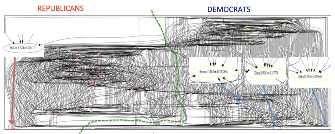
Given that LIGs belong to the class of 2-action graphical games [Kearns et al., 2001] with parametric payoff functions, we first needed to deal with the relative dearth of work on the broader problem of learning general graphical games from purely behavioral data. Hence, in addressing this problem, while inspired by the computational approach of Irfan and Ortiz [2014], the learning problem formulation we propose is in principle applicable to arbitrary games (although, again, the emphasis is on the PSNE of such games). In particular, we introduce a simple statistical generative mixture model, built “on top of” the game-theoretic model, with the only objective being to capture noise in the data. Despite the simplicity of the generative model, we are able to learn games from U.S. congressional voting records, which we use as a source of real-world behavioral data, that, as we will illustrate, seem to capture interesting, non-trivial aspects of the U.S. congress. While such models learned from real-world data are impossible to validate, we argue that there exists a considerable amount of anecdotal evidence for such aspects as captured by the models we learned. Figure 1 provides a brief illustration. (Should there be further need for clarification as to the why we present this figure, please see Footnote 14.)
As a final remark, given that LIGs constitute a non-trivial sub-class of parametric graphical games, we view our work as a step in the direction of addressing the broader problem of learning general graphical games with a large number of players from strictly behavioral data. We also hope our work helps to continue to bring and increase attention from the machine-learning community to the problem of inferring games from behavioral data (in which we attempt to learn a game that would “rationalize” players’ observed behavior).777This is a type of problem arising from game theory and economics that is different from the problem of learning in games (in which the focus is the study of how individual players learn to play a game by a sequence of repeated interactions), a more matured and perhaps better known problem within machine learning (see, e.g., Fudenberg and Levine 1999).
1.1 A Framework for Learning Games: Desiderata
The following list summarizes the discussion above and guides our choices in our pursuit of a machine-learning framework for learning game-theoretic graphical models from strictly behavioral data.
-
•
The learning algorithm
-
–
must output an LIG (which is a special type of graphical game); and
-
–
should be practical and tractably deal with a large number of players (typically in the hundreds, and certainly at least ).
-
–
-
•
The learned model objective is the “bottom line” in the sense that the basis for its evaluation is the prediction of end-state (or steady-state) joint decision-making behavior, and not the temporal behavioral dynamics that might have lead to end-state or the stable steady-state joint behavior.888Note that we are in no way precluding dynamic models as a way to end-state prediction. But there is no inherent need to make any explicit attempt or effort to model or predict the temporal behavioral dynamics that might have lead to end-state or the stable steady-state joint behavior, including pre-play “cheap talk,” which are often overly complex processes. (See Appendix A.1 for further discussion.)
-
•
The learning framework
-
–
would only have available strictly behavioral data on actual decisions/actions taken. It cannot require or use any kind of payoff-related information.
-
–
should be agnostic as to the type or nature of the decision-maker and does not assume each player is a single human. Players can be institutions or governments, or associated with the decision-making process of a group of individuals representing, e.g., a company (or sub-units, office sites within a company, etc.), a nation state (like in the UN, NATO, etc.), or a voting district. In other words, the recorded behavioral actions of each player may really be a representative of larger entities or groups of individuals, not necessarily a single human.
-
–
must provide computationally efficient learning algorithm with provable guarantees: worst-case polynomial running time in the number of players.
-
–
should be “data efficient” and provide provable guarantees on sample complexity (given in terms of “generalization” bounds).
-
–
1.2 Technical Contributions
While our probabilistic model is inspired by the concept of equilibrium from game theory, our technical contributions are not in the field of game theory nor computational game theory. Our technical contributions and the tools that we use are the ones in classical machine learning.
Our technical contributions include a novel generative model of behavioral data in Section 4 for general games. Motivated by the LIGs and the computational game-theoretic framework put forward by Irfan and Ortiz [2014], we formally define “identifiability” and “triviality” within the context of non-cooperative graphical games based on PSNE as the solution concept for stable outcomes in large strategic systems. We provide conditions that ensure identifiability among non-trivial games. We then present the maximum-likelihood estimation (MLE) problem for general (non-trivial identifiable) games. In Section 5, we show a generalization bound for the MLE problem as well as an upper bound of the functional/strategic complexity (i.e., analogous to the“VC-dimension” in supervised learning) of LIGs. In Section 6, we provide technical evidence justifying the approximation of the original problem by maximizing the number of observed equilibria in the data as suitable for a hypothesis-space of games with small true number of equilibria. We then present our convex loss minimization approach and a baseline sigmoidal approximation for LIGs. For completeness, we also present exhaustive search methods for both general games as well as LIGs. In Section 7, we formally define the concept of absolute-indifference of players and show that our convex loss minimization approach produces games in which all players are non-absolutely-indifferent. We provide a bound which shows that LIGs have small true number of equilibria with high probability.
2 Related Work
We provide a brief summary overview of previous work on learning games here, and delay discussion of the work presented below until after we formally present our model; this will provide better context and make “comparing and contrasting” easier for those interested, without affecting expert readers who may want to get to the technical aspects of the paper without much delay.
Table 1 constitutes our best attempt at a simple visualization to fairly present the differences and similarities of previous approaches to modeling behavioral data within the computational game-theory community in AI.
| Reference | Class | Needs | Learns | Learns | Guarant. | Equil. | Dyn. | Num. |
| Payoff | Param. | Struct. | Concept | Agents | ||||
| Wright and Leyton-Brown [2010] | NF | Y | Na | - | N | QRE | N | 2 |
| Wright and Leyton-Brown [2012] | NF | Y | Na | - | N | QRE | N | 2 |
| Gao and Pfeffer [2010] | NF | Y | Y | - | N | QRE | N | 2 |
| Vorobeychik et al. [2007] | NF | Y | Y | - | N | MSNE | N | 2-5 |
| Ficici et al. [2008] | NF | Y | Y | - | N | MSNE | N | 10-200 |
| Duong et al. [2008] | NGT | Y | Na | N | N | - | N | 4,10 |
| Duong et al. [2010] | NGTb | Y | Nc | N | N | - | Yd | 10 |
| Duong et al. [2012] | NGTb | Y | Nc | Ye | N | - | Yd | 36 |
| Duong et al. [2009] | GG | Y | Y | Yf | N | PSNE | N | 2-13 |
| Kearns and Wortman [2008] | NGT | N | - | - | Y | - | Y | 100 |
| Ziebart et al. [2010] | NF | N | Y | - | N | CE | N | 2-3 |
| Waugh et al. [2011] | NF | N | Y | - | Y | CE | Y | 7 |
| Our approach | GG | N | Y | Yg | Y | PSNE | N | 100g |
The research interest of previous work varies in what they intend to capture in terms of different aspects of behavior (e.g., dynamics, probabilistic vs. strategic) or simply different settings/domains (i.e., modeling “real human behavior,” knowledge of achieved payoff or utility, etc.).
With the exception of Ziebart et al. [2010], Waugh et al. [2011], Kearns and Wortman [2008], previous methods assume that the actions as well as corresponding payoffs (or noisy samples from the true payoff function) are observed in the data. Our setting largely differs from Ziebart et al. [2010], Kearns and Wortman [2008] because of their focus on system dynamics, in which future behavior is predicted from a sequence of past behavior. Kearns and Wortman [2008] proposed a learning-theory framework to model collective behavior based on stochastic models.
Our problem is clearly different from methods in quantal response models [McKelvey and Palfrey, 1995, Wright and Leyton-Brown, 2010, 2012] and graphical multiagent models (GMMs) [Duong et al., 2008, 2010] that assume known structure and observed payoffs. Duong et al. [2012] learns the structure of games that are not graphical, i.e., the payoff depends on all other players. Their approach also assumes observed payoff and consider a dynamic consensus scenario, where agents on a network attempt to reach a unanimous vote. In analogy to voting, we do not assume the availability of the dynamics (i.e., the previous actions) that led to the final vote. They also use fixed information on the conditioning sets of neighbors during their search for graph structure. We also note that the work of Vorobeychik et al. [2007], Gao and Pfeffer [2010], Ziebart et al. [2010] present experimental validation mostly for 2 players only, 7 players in Waugh et al. [2011] and up to 13 players in Duong et al. [2009].
In several cases in previous work, researchers define probabilistic models using knowledge of the payoff functions explicitly (i.e., a Gibbs distribution with potentials that are functions of the players payoffs, regrets, etc.) to model joint behavior (i.e., joint pure-strategies); see, e.g., Duong et al. [2008, 2010, 2012], and to some degree also Wright and Leyton-Brown [2010, 2012]. It should be clear to the reader that this is not the same as our generative model, which is defined directly on the PSNE (or stable outcomes) of the game, which the players’ payoffs determine only indirectly.
In contrast, in this paper, we assume that the joint actions are the only observable information and that both the game graph structure and payoff functions are unknown, unobserved and unavailable. We present the first techniques for learning the structure and parameters of a non-trivial class of large-population graphical games from joint actions only. Furthermore, we present experimental validation in games of up to players. Our convex loss minimization approach could potentially be applied to larger problems since it has polynomial time complexity in the number of players.
2.1 On Learning Probabilistic Graphical Models
There has been a significant amount of work on learning the structure of probabilistic graphical models from data. We mention only a few references that follow a maximum likelihood approach for Markov random fields [Lee et al., 2007], bounded tree-width distributions [Chow and Liu, 1968, Srebro, 2001], Ising models [Wainwright et al., 2007, Banerjee et al., 2008, Höfling and Tibshirani, 2009], Gaussian graphical models [Banerjee et al., 2006], Bayesian networks [Guo and Schuurmans, 2006, Schmidt et al., 2007b] and directed cyclic graphs [Schmidt and Murphy, 2009].
Our approach learns the structure and parameters of games by maximum likelihood estimation on a related probabilistic model. Our probabilistic model does not fit into any of the types described above. Although a (directed) graphical game has a directed cyclic graph, there is a semantic difference with respect to graphical models. Structure in a graphical model implies a factorization of the probabilistic model. In a graphical game, the graph structure implies strategic dependence between players, and has no immediate probabilistic implication. Furthermore, our general model differs from Schmidt and Murphy [2009] since our generative model does not decompose as a multiplication of potential functions.
Finally, it is very important to note that our specific aim is to model behavioral data that is strategic in nature. Hence, our modeling and learning approach deviates from those for probabilistic graphical models which are of course better suited for other types of data, mostly probabilistic in nature (i.e., resulting from a fixed underlying probability distribution). As a consequence, it is also very important to keep in mind that our work is not in competition with the work in probabilistic graphical models, and is not meant to replace it (except in the context of data sets collected from complex strategic behavior just mentioned). Each approach has its own aim, merits and pitfalls in terms of the nature of data sets that each seeks to model. We return to this point in Section 8 (Experimental Results).
2.2 On Linear Threshold Models and Econometrics
Irfan and Ortiz [2014] introduced LIGs in the AI community, showed that such games are useful, and addressed a variety of computational problems, including the identification of most influential senators. The class of LIGs is related to the well-known linear threshold model (LTM) in sociology [Granovetter, 1978], recently very popular within the social network and theoretical computer science community [Kleinberg, 2007].999López-Pintado and Watts [2008] also provide an excellent summary of the various models in this area of mathematical social science. Irfan and Ortiz [2014] discusses linear threshold models in depth; we briefly discuss them here for self-containment. LTMs are usually studied as the basis for some kind of diffusion process. A typical problem is the identification of most influential individuals in a social network. An LTM is not in itself a game-theoretic model and, in fact, Granovetter himself argues against this view in the context of the setting and the type of questions in which he was most interested [Granovetter, 1978]. Our reading of the relevant literature suggests that subsequent work on LTMs has not taken a strictly game-theoretic view either. The problem of learning mathematical models of influence from behavioral data has just started to receive attention. There has been a number of articles in the last couple of years addressing the problem of learning the parameters of a variety of diffusion models of influence [Saito et al., 2008, 2009, 2010, Goyal et al., 2010, Gomez Rodriguez et al., 2010, Cao et al., 2011].101010Often learning consists of estimating the threshold parameter from data given as temporal sequences from“traces” or “action logs.” Sometimes the “influence weights” are estimated assuming a given graph, and almost always the weights are assumed positive and estimated as “probabilities of influence.” For example, Saito et al. [2010] considers a dynamic (continuous time) LTM that has only positive influence weights and a randomly generated threshold value. Cao et al. [2011] uses active learning to estimate the threshold values of an LTM leading to a maximum spread of influence.
Our model is also related to a particular model of discrete choice with social interactions in econometrics (see, e.g. Brock and Durlauf 2001). The main difference is that we take a strictly non-cooperative game-theoretic approach within the classical “static”/one-shot game framework and do not use a random utility model. We follow the approach of Irfan and Ortiz [2014] who takes a strictly non-cooperative game-theoretic approach within the classical “static”/one-shot game framework, and thus we do not use a random utility model. In addition, we do not make the assumption of rational expectations, which in the context of models of discrete choice with social interactions essentially implies the assumption that all players use exactly the same mixed strategy.111111A formal definition of “rational expectations” is beyond the scope of this paper. We refer the reader to the early part of the article by Brock and Durlauf [2001] where they explain why assuming rational expectations leads to the conclusion that all players use exactly the same mixed strategy. That is the relevant part of that work to ours.
3 Background: Game Theory and Linear Influence Games
In classical game-theory (see, e.g. Fudenberg and Tirole 1991 for a textbook introduction), a normal-form game is defined by a set of players (e.g., we can let if there are players), and for each player , a set of actions, or pure-strategies , and a payoff function mapping the joint actions of all the players, given by the Cartesian product , to a real number. In non-cooperative game theory we assume players are greedy, rational and act independently, by which we mean that each player always want to maximize their own utility, subject to the actions selected by others, irrespective of how the optimal action chosen help or hurt others.
A core solution concept in non-cooperative game theory is that of an Nash equilibrium. A joint action is a pure-strategy Nash equilibrium (PSNE) of a non-cooperative game if, for each player , ; that is, constitutes a mutual best-response, no player has any incentive to unilaterally deviate from the prescribed action , given the joint action of the other players in the equilibrium. In what follows, we denote a game by , and the set of all pure-strategy Nash equilibria of by121212Because this paper concerns mostly PSNE, we denote the set of PSNE of game as to simplify notation.
A (directed) graphical game is a game-theoretic graphical model [Kearns et al., 2001]. It provides a succinct representation of normal-form games. In a graphical game, we have a (directed) graph in which each node in corresponds to a player in the game. The interpretation of the edges/arcs of is that the payoff function of player is only a function of the set of parents/neighbors in (i.e., the set of players corresponding to nodes that point to the node corresponding to player in the graph). In the context of a graphical game, we refer to the ’s as the local payoff functions/matrices.
Linear influence games (LIGs) [Irfan and Ortiz, 2014] are a sub-class of -action graphical games with parametric payoff functions. For LIGs, we assume that we are given a matrix of influence weights , with , and a threshold vector . For each player , we define the influence function and the payoff function . We further assume binary actions: for all . The best response of player to the joint action of the other players is defined as
Intuitively, for any other player , we can think of as a weight parameter quantifying the “influence factor” that has on , and we can think of as a threshold parameter quantifying the level of “tolerance” that player has for playing .131313As we formally/mathematically define here, LIGs are -action graphical games with linear-quadratic payoff functions. Given our main interest in this paper on the PSNE solution concept, for the most part, we simply view LIGs as compact representations of the PSNE of graphical games that the algorithms of Irfan and Ortiz [2014] use for CSI. (This is in contrast to a perhaps more natural, “intuitive” but still informal description/interpretation one may provide for instructive/pedagogical purposes based on “direct influences,” as we do here.) This view of LIGs is analogous to the modern, predominant view of Bayesian networks as compact representations of joint probability distributions that are also very useful for modeling uncertainty in complex systems and practical for probabilistic inference [Koller and Friedman, 2009]. (And also analogous is the “intuitive” descriptions/interpretations of BN structures, used for instructive/pedagogical purposes, based on “causal” interactions between the random variables Koller and Friedman, 2009.)
As discussed in Irfan and Ortiz [2014], LIGs are also a sub-class of polymatrix games [Janovskaja, 1968]. Furthermore, in the special case of and symmetric , a LIG becomes a party-affiliation game [Fabrikant et al., 2004].
In this paper, the use of the verb “influence” strictly refers to influences defined by the model.
Figure 1 provides a preview illustration of the application of our approach to congressional voting.141414We present this game graph because many people express interest in “seeing” the type of games we learn on this particular data set. The reader should please understand that by presenting this graph we are definitely not implying or arguing that we can identify the ground-truth graph of “direct influences.” (We say this even in the very unlikely event that the “ground-truth model” be an LIG that faithfully capture the “true direct influences” in this U.S. Congress, something arguably no model could ever do.) As we show later in Section 4.2, LIGs are not identifiable with respect to their local compact parametric representation encoding the game graph through their weights and biases, but only with respect to their PSNE, which are joint actions capturing a global property of a game that we really care about for CSI. Certainly, we could never validate the model parameters of an LIG at the local, microscopic level of “direct influences” using only the type of observational data we used to learn the model depicted by the graph in the figure. For that, we would need help from domain experts to design controlled experiments that would yield the right type of data for proper/rigorous scientific validation.
4 Our Proposed Framework for Learning LIGs
Our goal is to learn the structure and parameters of an LIG from observed joint actions only (i.e., without any payoff data/information).151515In principle, the learning framework itself is technically immediately/easily applicable to any class of simultaneous/one-shot games. Generalizing the algorithms and other theoretical results (e.g., on generalization error) while maintaining the tractability in sample complexity and computation may require significant effort. Yet, for simplicity, most of the presentation in this section is actually in terms of general 2-action games. While we make sporadic references to LIGs throughout the section, it is not until we reach the end of the section that we present and discuss the particular instantiation of our proposed framework with LIGs.
Our main performance measure will be average log-likelihood (although later we will be considering misclassification-type error measures in the context of simultaneous-classification, as a result of an approximation of the average log-likelihood). Our emphasis on a PSNE-based statistical model for the behavioral data results from the approach to causal strategic inference taken by Irfan and Ortiz [2014], which is strongly founded on PSNE.161616The possibility that PSNE may not exist in some LIGs does not present a significant problem in our case because we are learning the game, and can require that the LIG output has at least one PSNE. Indeed, in our approach, games with no PSNE achieve the lowest possible likelihood within our generative model of the data; said differently, games with PSNE have higher likelihoods than those that do not have any PSNE.
Note that our problem is unsupervised, i.e., we do not know a priori which joint actions are PSNE and which ones are not. If our only goal were to find a game in which all the given observed data is an equilibrium, then any “dummy” game, such as the “dummy” LIG , would be an optimal solution because .171717Ng and Russell [2000] made a similar observation in the context of single-agent inverse reinforcement learning (IRL). In this section, we present a probabilistic formulation that allows finding games that maximize the empirical proportion of equilibria in the data while keeping the true proportion of equilibria as low as possible. Furthermore, we show that trivial games such as LIGs with , obtain the lowest log-likelihood.
4.1 Our Proposed Generative Model of Behavioral Data
We propose the following simple generative (mixture) model for behavioral data based strictly in the context of “simultaneous”/one-shot play in non-cooperative game theory, again motivated by Irfan and Ortiz [2014]’s PSNE-based approach to causal strategic inference (CSI).181818Model “simplicity” and “abstractions” are not necessarily a bad thing in practice. More “realism” often leads to more “complexity” in terms of model representation and computation; and to potentially poorer generalization performance as well [Kearns and Vazirani, 1994]. We believe that even if the data could be the result of complex cognitive, behavioral or neuronal processes underlying human decision making and social interactions, the practical guiding principle of model selection in ML, which governs the fundamental tradeoff between model complexity and generalization performance, still applies. Let be a game. With some probability , a joint action is chosen uniformly at random from ; otherwise, is chosen uniformly at random from its complement set . Hence, the generative model is a mixture model with mixture parameter corresponding to the probability that a stable outcome (i.e., a PSNE) of the game is observed, uniform over PSNE. Formally, the probability mass function (PMF) over joint-behaviors parameterized by is
| (1) |
where we can think of as the “signal” level, and thus as the “noise” level in the data set.
Remark 1.
Note that in order for Eq. (1) to be a valid PMF for any , we need to enforce the following conditions and . Furthermore, note that in both cases () the PMF becomes a uniform distribution. We also enforce the following condition:191919We can easily remove this condition at the expense of complicating the theoretical analysis on the generalization bounds because of having to deal with those extreme cases. if then .
4.2 On PSNE-Equivalence and PSNE-Identifiability of Games
For any valid value of mixture parameter , the PSNE of a game completely determines our generative model . Thus, given any such mixture parameter, two games with the same set of PSNE will induce the same PMF over the space of joint actions.202020It is not hard to come up with examples of multiple games that have the same PSNE set. In fact, later in this section, we show three instances of LIGs with very different weight-matrix parameter that have this property. Note that this is not a roadblock to our objectives of learning LIGs because our main interest is the PSNE of the game, not the individual parameters that define it. We note that this situation is hardly exclusive to game-theoretic models: an analogous issue occurs in probabilistic graphical models (e.g., Bayesian networks).
Definition 2.
We say that two games and are PSNE-equivalent if and only if their PSNE sets are identical, i.e., .
We often drop the “PSNE-” qualifier when clear from context.
Definition 3.
We say a set of valid parameters for the generative model is PSNE-identifiable with respect to the PMF defined in Eq. (1), if and only if, for every pair , if for all then and . We say a game is PSNE-identifiable with respect to and the , if and only if, there exists a such that .
Definition 4.
We define the true proportion of equilibria in the game relative to all possible joint actions as
| (2) |
We also say that a game is trivial if and only if (or equivalently ), and non-trivial if and only if (or equivalently ).
The following propositions establish that the condition ensures that the probability of an equilibrium is strictly greater than a non-equilibrium. The condition also guarantees that non-trivial games are identifiable.
Proposition 5.
Given a non-trivial game , the mixture parameter if and only if for any and .
Proof.
Note that and given Eq. (2), we prove our claim. ∎
Proposition 6.
Let and be two valid generative-model parameter tuples.
-
(a)
If and then ,
-
(b)
Let and be also two non-trivial games such that and . If , then and .
Proof.
The last proposition, along with our definitions of “trivial” (as given in Definition 4) and “identifiable” (Definition 3), allows us to formally define our hypothesis space.
Definition 7.
Let be a class of games of interest. We call the set the hypothesis space of non-trivial identifiable games and mixture parameters. We also refer to a game that is also in some tuple for some , as a non-trivial identifiable game.212121Technically, we should call the set “the hypothesis space consisting of tuples of non-trivial games from and mixture parameters identifiable up to PSNE, with respect to the probabilistic model defined in Eq. (1).” Similarly, we should call such game “a non-trivial game from identifiable up to PSNE, with respect to the probabilistic model defined in Eq. (1).” We opted for brevity.
Remark 8.
Recall that a trivial game induces a uniform PMF by Remark 1. Therefore, a non-trivial game is not equivalent to a trivial game since by Proposition 5, non-trivial games do not induce uniform PMFs.222222In general, Section 4.2 characterizes our hypothesis space (non-trivial identifiable games and mixture parameters) via two specific conditions. The first condition, non-triviality (explained in Remark 1), is . The second condition, identifiability of the PSNE set from its related PMF (discussed in Propositions 5 and 6), is . For completeness, in this remark, we clarify that the class of trivial games (uniform PMFs) is different from the class of non-trivial games (non-uniform PMFs). Thus, in the rest of the paper we focus exclusively on non-trivial identifiable games; that is, games that produce non-uniform PMFs and for which the PSNE set is uniquely identified from their PMFs.
4.3 Additional Discussion on Modeling Choices
We now discuss other equilibrium concepts, such as mixed-strategy Nash equilibria (MSNE) and quantal response equilibria (QRE). We also discuss a more sophisticated noise process as well as a generalization of our model to non-uniform distributions; while likely more realistic, the alternative models are mathematically more complex and potentially less tractable computationally.
4.3.1 On Other Equilibrium Concepts
There is still quite a bit of debate as to the appropriateness of game-theoretic equilibrium concepts to model individual human behavior in a social context. Camerer’s book on behavioral game theory [Camerer, 2003] addresses some of the issues. Our interpretation of Camerer’s position is not that Nash equilibria is universally a bad predictor but that it is not consistently the best, for reasons that are still not well understood. This point is best illustrated in Chapter 3, Figure 3.1 of Camerer [2003].
(Logit) quantal response equilibria (QRE) [McKelvey and Palfrey, 1995] has been proposed as an alternative to Nash in the context of behavioral game theory. Models based on QRE have been shown superior during initial play in some experimental settings, but prior work assumes known structure and observed payoffs, and only the “precision/rationality parameter” is estimated, e.g. Wright and Leyton-Brown [2010, 2012]. In a logit QRE, the precision parameter, typically denoted by , can be mathematically interpreted as the inverse-temperature parameter of individual Gibbs distributions over the pure-strategy of each player .
It is customary to compute the MLE for from available data. To the best of our knowledge, all work in QRE assumes exact knowledge of the game payoffs, and thus, no method has been proposed to simultaneously estimate the payoff functions when they are unknown. Indeed, computing MLE for , given the payoff functions, is relatively efficient for normal-form games using standard techniques, but may be hard for graphical games; on the other hand, MLE estimation of the payoff functions themselves within a QRE model of behavior seems like a highly non-trivial optimization problem, and is unclear that it is even computationally tractable, even in normal-form games. At the very least, standard techniques do not apply and more sophisticated optimization algorithms or heuristics would have to be derived. Such extensions are clearly beyond the scope of this paper.232323Note that despite the apparent similarity in mathematical expression between logit QRE and the PSNE of the LIG we obtain by using individual logistic regression, they are fundamentally different because of the complex correlations that QRE conditions impose on the parameters of the payoff functions. It is unclear how to adapt techniques for logistic regression similar to the ones we used here to efficiently/tractably compute MLE within the logit QRE framework.
Wright and Leyton-Brown [2012] also considers even more mathematically complex variants of behavioral models that combine QRE with different models that account for constraints in “cognitive levels” of reasoning ability/effort, yet the estimation and usage of such models still assumes knowledge of the payoff functions.
It would be fair to say that most of the human-subject experiments in behavioral game theory involve only a handful of players [Camerer, 2003]. The scalability of those results to games with a large population of players is unclear.
Now, just as an example, we do not necessarily view the Senators final votes as those of a single human individual anyway: after all, such a decision is (or should be) obtained with consultation with their staff and (one would at least hope) the constituency of the state they represent. Also, the final voting decision is taken after consultation or meetings between the staff of the different senators. We view this underlying process as one of “cheap talk.” While cheap talk may be an important process to study, in this paper, we just concentrate on the end result: the final vote. The reason is more than just scientific; as the congressional voting setting illustrates, data for such process is sometimes not available, or would seem very hard to infer from the end-states alone. While our experiments concentrate on congressional voting data, because it is publicly available and easy to obtain, the same would hold for other settings such as Supreme court decisions, voluntary vaccination, UN voting records and governmental decisions, to name a few. We speculate that in almost all those cases, only the end-result is likely to be recorded and little information would be available about the “cheap talk” process or “pre-play” period leading to the final decision.
In our work we consider PSNE because of our motivation to provide LIGs for use within the casual strategic inference framework for modeling “influence” in large-population networks of Irfan and Ortiz [2014]. Note that the universality of MSNE does not diminish the importance of PSNE in game theory.242424Research work on the properties and computation of PSNE include Rosenthal [1973], Gilboa and Zemel [1989], Stanford [1995], Rinott and Scarsini [2000], Fabrikant et al. [2004], Gottlob et al. [2005], Sureka and Wurman [2005], Daskalakis and Papadimitriou [2006], Dunkel [2007], Dunkel and Schulz [2006], Dilkina et al. [2007], Ackermann and Skopalik [2007], Hasan et al. [2008], Hasan and Galiana [2008], Ryan et al. [2010], Chapman et al. [2010], Hasan and Galiana [2010]. Indeed, a debate still exist within the game theory community as to the justification for randomization, specially in human contexts. While concentrating exclusively on PSNE may not make sense in all settings, it does make sense in some.252525For example, in the context of congressional voting, we believe Senators almost always have full-information about how some, if not all other Senators they care about would vote. Said differently, we believe uncertainty in a Senator’s final vote, by the time the vote is actually taken, is rare, and certainly not the norm. Hence, it is unclear how much there is to gain, in this particular setting, by considering possible randomization in the Senators’ voting strategies. In addition, were we to introduce mixed-strategies into the inference and learning framework and model, we would be adding a considerable amount of complexity in almost all respects, thus requiring a substantive effort to study on its own.262626For example, note that because in our setting we learn exclusively from observed joint actions, we could not assume knowledge of the internal mixed-strategies of players. Perhaps we could generalize our model to allow for mixed-strategies by defining a process in which a joint mixed strategy from the set of MSNE (or its complement) is drawn according to some distribution, then a (pure-strategy) realization is drawn from that would correspond to the observed joint actions. One problem we might face with this approach is that little is known about the structure of MSNE in general multi-player games. For example, it is not even clear that the set of MSNE is always measurable in general!
4.3.2 On the Noise Process
Here we discuss a more sophisticated noise process as well as a generalization of our model to non-uniform distributions. The problem with these models is that they lead to a significantly more complex expression for the generative model and thus likelihood functions. This is in contrast to the simplicity afforded us by the generative model with a more global noise process defined above. (See Appendix A.2.1 for further discussion.)
In this paper we considered a “global” noise process, modeled using a parameter corresponding to the probability that a sample observation is an equilibrium of the underlying hidden game. One could easily envision potentially better and more natural/realistic “local” noise processes, at the expense of producing a significantly more complex generative model, and less computationally amenable, than the one considered in this paper. For instance, we could use a noise process that is formed of many independent, individual noise processes, one for each player. (See Appendix A.2.2 for further discussion.)
4.4 Learning Games via MLE
We now formulate the problem of learning games as one of maximum likelihood estimation with respect to our PSNE-based generative model defined in Eq. (1) and the hypothesis space of non-trivial identifiable games and mixture parameters (Definition 7). We remind the reader that our problem is unsupervised; that is, we do not know a priori which joint actions are equilibria and which ones are not. We base our framework on the fact that games are PSNE-identifiable with respect to their induced PMF, under the condition that , by Proposition 6.
First, we introduce a shorthand notation for the Kullback-Leibler (KL) divergence between two Bernoulli distributions parameterized by and :
| (3) |
Using this function, we can derive the following expression of the MLE problem.
Lemma 9.
Given a data set , define the empirical proportion of equilibria, i.e., the proportion of samples in that are equilibria of , as
| (4) |
The MLE problem for the probabilistic model given in Eq. (1) can be expressed as finding:
| (5) |
where and are as in Definition 7, and is defined as in Eq. (2). Also, the optimal mixture parameter .
Proof.
Let , and . First, for a non-trivial , for , and for . The average log-likelihood . By adding , this can be rewritten as , and by using Eq. (3) we prove our claim.
Note that by maximizing with respect to the mixture parameter and by properties of the KL divergence, we get . We define our hypothesis space given the conditions in Remark 1 and Propositions 5 and 6. For the case , we “shrink” the optimal mixture parameter to in order to enforce the second condition given in Remark 1. ∎
Remark 10.
Furthermore, Eq. (5) implies that for non-trivial identifiable games , we expect the true proportion of equilibria to be strictly less than the empirical proportion of equilibria in the given data. This is by setting the optimal mixture parameter and the condition in our hypothesis space.
4.4.1 Learning LIGs via MLE: Model Selection
Our main learning problem consists of inferring the structure and parameters of an LIG from data with the main purpose being modeling the game’s PSNE, as reflected in the generative model. Note that, as we have previously stated, different games (i.e., with different payoff functions) can be PSNE-equivalent. For instance, the three following LIGs, with different weight parameter matrices, induce the same PSNE sets, i.e., for :272727Using the formal mathematical definition of “identifiability” in statistics, we would say that the LIG examples prove that the model parameters of an LIG are not identifiable with respect to the generative model defined in Eq. (1). We note that this situation is hardly exclusive to game-theoretic models. As example of an analogous issue in probabilistic graphical models is the fact that two Bayesian networks with different graph structures can represent not only the same conditional independence properties but also exactly the same set of joint probability distributions [Chickering, 2002, Koller and Friedman, 2009]. As a side note, we can distinguish these games with respect to their larger set of mixed-strategy Nash equilibria (MSNE), but, as stated previously, we do not consider MSNE in this paper because our primary motivation is the work of Irfan and Ortiz [2014], which is based on the concept of PSNE.
Thus, not only the MLE may not be unique, but also all such PSNE-equivalent MLE games will achieve the same level of generalization performance. But, as reflected by our generative model, our main interest in the model parameters of the LIGs is only with respect to the PSNE they induce, not the model parameters per se. Hence, all we need is a way to select among PSNE-equivalent LIGs.
In our work, the indentifiability or interpretability of exact model parameters of LIGs is not our main interest. That is, in the research presented here, we did not seek or attempt to work on creating alternative generative models with the objective to provide a theoretical guarantee that, given an infinite amount of data, we can recover the model parameters of an unknown ground-truth model generating the data, assuming the ground-truth model is an LIG. We opted for a more practical ML approach in which we just want to learn a single LIG that has good generalization performance (i.e., predictive performance in terms of average log-likelihood) with respect to our generative model. Given the nature of our generative model, this essentially translate to learning an LIG that captures as best as possible the PSNE of the unknown ground-truth game. Unfortunately, as we just illustrated, several LIGs with different model parameter values can have the same set of PSNE. Thus, they all would have the same (generalization) performance ability.
As we all know, model selection is core to ML. One of the reason we chose an ML-approach to learning games is precisely the elegant way in which ML deals with the problem of how to select among multiple models that achieve the same level of performance: invoke the principle of Ockham’s razor and select the “simplest” model among those with the same (generalization) performance. This ML philosophy is not ad hoc. It is instead well established in practice and well supported by theory. Seminal results from the various theories of learning, such as computational and statistical learning theory and PAC learning, support the well-known ML adage that “learning requires bias.” In short, as is by now standard in an ML-approach, we measure the quality of our data-induced models via their generalization ability and invoke the principle of Ockham’s razor to bias our search toward simpler models using well-known and -studied regularization techniques.
Now, as we also all know, exactly what “simple” and “bias” means depends on the problem. In our case, we would prefer games with sparse graphs, if for no reason other than to simplify analysis, exploration, study, and (visual) “interpretability” of the game model by human experts, everything else being equal (i.e., models with the same explanatory power on the data as measured by the likelihoods).282828Just to be clear, here we mean “interpretability” not in any formal mathematical sense, or as often used in some areas of the social sciences such as economics. But, instead, as we typically use it in ML/AI textbooks, such as for example, when referring to shallow/sparse decision trees, generally considered to be easier to explain and understand. Similarly, the hope here is that the “sparsity” or “simplicity” of the game graph/model would make it also simpler for human experts to explain or understand what about the model is leading them to generate novel hypotheses, reach certain conclusions or make certain inferences about the global strategic behavior of the agents/players, such as those based on the game’s PSNE and facilitated by CSI. We should also point out that, in preliminary empirical work, we have observed that the representationally sparser the LIG graph, the computationally easier it is for algorithms and other heuristics that operate on the LIG, as those of Irfan and Ortiz [2014] for CSI, for example. For example, among the LIGs presented above, using structural properties alone, we would generally prefer the former two models to the latter, all else being equal (e.g., generalization performance).
5 Generalization Bound and VC-Dimension
In this section, we show a generalization bound for the maximum likelihood problem as well as an upper bound of the VC-dimension of LIGs. Our objective is to establish that with probability at least , for some confidence parameter , the maximum likelihood estimate is within of the optimal parameters, in terms of achievable expected log-likelihood.
Given the ground-truth distribution of the data, let be the expected proportion of equilibria, i.e.,
and let be the expected log-likelihood of a generative model from game and mixture parameter , i.e.,
Let be a maximum-likelihood estimate as in Eq. (5) (i.e., ), and be the maximum-expected-likelihood estimate: .292929If the ground-truth model belongs to the class of LIGs, then is also the ground-truth model, or PSNE-equivalent to it. We use, without formally re-stating, the last definitions in the technical results presented in the remaining of this section.
Note that our hypothesis space as stated in Definition 7 includes a continuous parameter that could potentially have infinite VC-dimension. The following lemma will allow us later to prove that uniform convergence for the extreme values of implies uniform convergence for all in the domain.
Lemma 11.
Consider any game and, for , let , and . If, for any we have and , then .
Proof.
Let , , , , and and be the expectation and probability with respect to the ground-truth distribution of the data.
First note that for any , we have .
Similarly, for any , we have . So that .
Furthermore, the function is strictly monotonically increasing for . If then . Else, if , we have . Finally, if then . ∎
In the remaining of this section, denote by the number of all possible PSNE sets induced by games in , the class of games of interest.
The following theorem shows that the expected log-likelihood of the maximum likelihood estimate converges in probability to that of the optimal , as the data size increases.
Theorem 12.
The following holds with -probability at least :
Proof.
First our objective is to find a lower bound for .
Let . Now, we have . The last equality follows from invoking Lemma 11.
Note that and that since , the log-likelihood is bounded as , where . Therefore, by Hoeffding’s inequality, we have .
Furthermore, note that there are possible parameters , since we need to consider only two values of and because the number of all possible PSNE sets induced by games in is . Therefore, by the union bound we get the following uniform convergence . Finally, by solving for we prove our claim. ∎
Remark 13.
A more elaborate analysis allows to tighten the bound in Theorem 12 from to . We chose to provide the former result for clarity of presentation.
The following theorem establishes the complexity of the class of LIGs, which implies that the term of the generalization bound in Theorem 12 is only polynomial in the number of players .
Theorem 14.
If is the class of LIGs, then .
Proof.
The logarithm of the number of possible pure-strategy Nash equilibria sets supported by (i.e., that can be produced by some game in ) is upper bounded by the VC-dimension of the class of neural networks with a single hidden layer of units and input units, linear threshold activation functions, and constant output weights.
For every LIG in , define the neural network with a single layer of hidden units, of the inputs corresponds to the linear terms and corresponds to the quadratic polynomial terms for all pairs of players , . For every hidden unit , the weights corresponding to the linear terms are , respectively, while the weights corresponding to the quadratic terms are , for all pairs of players , , respectively. The weights of the bias term of all the hidden units are set to . All output weights are set to while the weight of the output bias term is set to . The output of the neural network is . Note that we define the neural network to classify non-equilibrium as opposed to equilibrium to keep the convention in the neural network literature to define the threshold function to output for input . The alternative is to redefine the threshold function to output instead for input .
Finally, we use the VC-dimension of neural networks [Sontag, 1998]. ∎
Corollary 15.
The following holds with -probability at least :
where is the class of LIGs, in which case (Definition 7) becomes the hypothesis space of non-trivial identifiable LIGs and mixture parameters.
6 Algorithms
In this section, we approximate the maximum likelihood problem by maximizing the number of observed equilibria in the data, suitable for a hypothesis space of games with small true proportion of equilibria. We then present our convex loss minimization approach. We also discuss baseline methods such as sigmoidal approximation and exhaustive search.
But first, let us discuss some negative results that justifies the use of simple approaches. Irfan and Ortiz [2014] showed that counting the number of Nash equilibria in LIGs is #P-complete; thus, computing the log-likelihood function, and therefore MLE, is NP-hard.303030This is not a disadvantage relative to probabilistic graphical models, since computing the log-likelihood function is also NP-hard for Ising models and Markov random fields in general, while learning is also NP-hard for Bayesian networks. General approximation techniques such as pseudo-likelihood estimation do not lead to tractable methods for learning LIGs.313131We show that evaluating the pseudo-likelihood function for our generative model is NP-hard. Consider a non-trivial LIG . Furthermore, assume has a single non-absolutely-indifferent player and absolutely-indifferent players ; that is, assume that and (See Definition 19). Let , we have and therefore . The result follows because computing is #P-complete, even for this specific instance of a single non-absolutely-indifferent player [Irfan and Ortiz, 2014]. From an optimization perspective, the log-likelihood function is not continuous because of the number of equilibria. Therefore, we cannot rely on concepts such as Lipschitz continuity.323232To prove that counting the number of equilibria is not (Lipschitz) continuous, we show how small changes in the parameters can produce big changes in . For instance, consider two games , where and for . For , any -norm but remains constant. Furthermore, bounding the number of equilibria by known bounds for Ising models leads to trivial bounds.333333The log-partition function of an Ising model is a trivial bound for counting the number of equilibria. To see this, let , , where denotes the partition function of an Ising model. Given the convexity of [Koller and Friedman, 2009], and that the gradient vanishes at , we know that , which is the maximum .
6.1 An Exact Quasi-Linear Method for General Games: Sample-Picking
As a first approach, consider solving the maximum likelihood estimation problem in Eq. (5) by an exact exhaustive search algorithm. This algorithm iterates through all possible Nash equilibria sets, i.e., for , we generate all possible sets of size with elements from the joint-action space . Recall that there exist of such sets of size and since the search space is super-exponential in the number of players .
Based on few observations, we can obtain an algorithm for samples. First, note that the above method does not constrain the set of Nash equilibria in any fashion. Therefore, only joint actions that are observed in the data are candidates of being Nash equilibria in order to maximize the log-likelihood. This is because the introduction of an unobserved joint action will increase the true proportion of equilibria without increasing the empirical proportion of equilibria and thus leading to a lower log-likelihood in Eq. (5). Second, given a fixed number of Nash equilibria , the best strategy would be to pick the joint actions that appear more frequently in the observed data. This will maximize the empirical proportion of equilibria, which will maximize the log-likelihood. Based on these observations, we propose Algorithm 1.
As an aside note, the fact that general games do not constrain the set of Nash equilibria, makes the method more likely to over-fit. On the other hand, LIGs will potentially include unobserved equilibria given the linearity constraints in the search space, and thus they would be less likely to over-fit.
6.2 An Exact Super-Exponential Method for LIGs: Exhaustive Search
Note that in the previous subsection, we search in the space of all possible games, not only the LIGs. First note that sample-picking for linear games is NP-hard, i.e., at any iteration of sample-picking, checking whether the set of Nash equilibria corresponds to an LIG or not is equivalent to the following constraint satisfaction problem with linear constraints:
| (6) |
Note that Eq. (6) contains “or” operators in order to account for the non-equilibria. This makes the problem of finding the that satisfies such conditions NP-hard for a non-empty complement set . Furthermore, since sample-picking only consider observed equilibria, the search is not optimal with respect to the space of LIGs.
Regarding a more refined approach for enumerating LIGs only, note that in an LIG each player separates hypercube vertices with a linear function, i.e., for and we have . Assume we assign a binary label to each vertex , then note that not all possible labelings are linearly separable. Labelings which are linearly separable are called linear threshold functions (LTFs). A lower bound of the number of LTFs was first provided in Muroga [1965], which showed that the number of LTFs is at least . Tighter lower bounds were shown later in Yamija and Ibaraki [1965] for and in Muroga and Toda [1966] for . Regarding an upper bound, Winder [1960] showed that the number of LTFs is at most . By using such bounds for all players, we can conclude that there is at least and at most LIGs (which is indeed another upper bound of the VC-dimension of the class of LIGs; the bound in Theorem 14 is tighter and uses bounds of the VC-dimension of neural networks). The bounds discussed above would bound the time-complexity of a search algorithm if we could easily enumerate all LTFs for a single player. Unfortunately, this seems to be far from a trivial problem. By using results in Muroga [1971], a weight vector with integer entries such that is sufficient to realize all possible LTFs. Therefore we can conclude that enumerating LIGs takes at most steps, and we propose the use of this method only for .
For we found that the number of possible PSNE sets induced by LIGs is 23,706. Experimentally, we did not find differences between this method and sample-picking since most of the time, the model with maximum likelihood was an LIG.
6.3 From Maximum Likelihood to Maximum Empirical Proportion of Equilibria
We approximately perform maximum likelihood estimation for LIGs, by maximizing the empirical proportion of equilibria, i.e., the equilibria in the observed data. This strategy allows us to avoid computing as in Eq. (2) for maximum likelihood estimation (given its dependence on ). We propose this approach for games with small true proportion of equilibria with high probability, i.e., with probability at least , we have for . Particularly, we will show in Section 7 that for LIGs we have . Given this, our approximate problem relies on a bound of the log-likelihood that holds with high probability. We also show that under very mild conditions, the parameters belong to the hypothesis space of the original problem with high probability.
First, we derive bounds on the log-likelihood function.
Lemma 16.
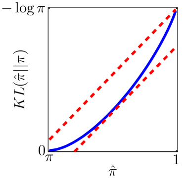
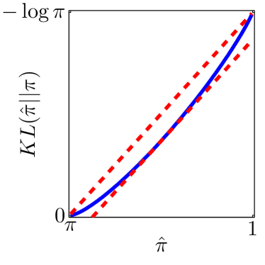
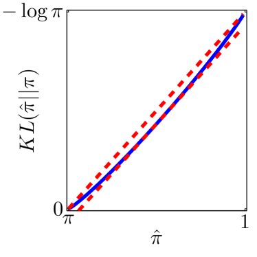
Given a non-trivial game with , the KL divergence in the log-likelihood function in Eq. (5) is bounded as follows:
Proof.
Let and . Note that ,343434Here we are making the implicit assumption that . This is sensible. For example, in most models learned from the congressional voting data using a variety of learning algorithms we propose, the total number of PSNE would range roughly from 100K—1M; using base 2, this is roughly from —. This may look like a huge number until one recognizes that there could potential be PSNE. Hence, we have that would be in the range of —. In fact, we believe this holds more broadly because, as a general objective, we want models that can capture as many PSNE behavior as possible but no more than needed, which tend to reduce the PSNE of the learned models, and thus their values, while simultaneously trying to increase as much as possible. and . Since the function is convex we can upper-bound it by .
To find a lower bound, we find the point in which the derivative of the original function is equal to the slope of the upper bound, i.e., , which gives . Then, the maximum difference between the upper bound and the original function is given by . ∎
Note that the lower and upper bounds are very informative when (or in our setting when ), since becomes small when compared to , as shown in Figure 2.
Next, we derive the problem of maximizing the empirical proportion of equilibria from the maximum likelihood estimation problem.
Theorem 17.
Assume that with probability at least we have for . Maximizing a lower bound (with high probability) of the log-likelihood in Eq. (5) is equivalent to maximizing the empirical proportion of equilibria:
| (7) |
furthermore, for all games such that for some , for sufficiently large and optimal mixture parameter , we have , where is the hypothesis space of non-trivial identifiable games and mixture parameters.
Proof.
By applying the lower bound in Lemma 16 in Eq. (5) to non-trivial games, we have . Since , we have . Therefore . Regarding the term , if , and if and approaches 0 when . Maximizing the lower bound of the log-likelihood becomes by removing the constant terms that do not depend on .
In order to prove we need to prove . For proving the first inequality , note that , and therefore has at least one equilibria. For proving the third inequality , note that . For proving the second inequality , we need to prove and . Since and , it suffices to prove . Similarly we need to prove . Putting both together, we have since and . Finally, . ∎
6.4 A Non-Concave Maximization Method: Sigmoidal Approximation
A very simple optimization approach can be devised by using a sigmoid in order to approximate the 0/1 function in the maximum likelihood problem of Eq. (5) as well as when maximizing the empirical proportion of equilibria as in Eq. (7). We use the following sigmoidal approximation:
| (8) |
The additional term ensures that for we get . We perform gradient ascent on these objective functions that have many local maxima. Note that when maximizing the “sigmoidal” likelihood, each step of the gradient ascent is NP-hard due to the “sigmoidal” true proportion of equilibria. Therefore, we propose the use of the sigmoidal maximum likelihood only for .
In our implementation, we add an -norm regularizer where to both maximization problems. The -norm regularizer encourages sparseness and attempts to lower the generalization error by controlling over-fitting.
6.5 Our Proposed Approach: Convex Loss Minimization
From an optimization perspective, it is more convenient to minimize a convex objective instead of a sigmoidal approximation in order to avoid the many local minima.
Note that maximizing the empirical proportion of equilibria in Eq. (7) is equivalent to minimizing the empirical proportion of non-equilibria, i.e., . Furthermore, . Denote by the 0/1 loss, i.e., . For LIGs, maximizing the empirical proportion of equilibria in Eq. (7) is equivalent to solving the loss minimization problem:
| (9) |
We can further relax this problem by introducing convex upper bounds of the 0/1 loss. Note that the use of convex losses also avoids the trivial solution of Eq. (9), i.e., (which obtains the lowest log-likelihood as discussed in Remark 10). Intuitively speaking, note that minimizing the logistic loss will make , while minimizing the hinge loss will make unlike the 0/1 loss that only requires in order to be minimized. In what follows, we develop four efficient methods for solving Eq. (9) under specific choices of loss functions, i.e., hinge and logistic.
In our implementation, we add an -norm regularizer where to all the minimization problems. The -norm regularizer encourages sparseness and attempts to lower the generalization error by controlling over-fitting.
6.5.1 Independent Support Vector Machines and Logistic Regression
We can relax the loss minimization problem in Eq. (9) by using the loose bound . This relaxation simplifies the original problem into several independent problems. For each player , we train the weights in order to predict independent (disjoint) actions. This leads to 1-norm SVMs of Bradley and Mangasarian [1998], Zhu et al. [2004] and -regularized logistic regression. We solve the latter with the -projection method of Schmidt et al. [2007a]. While the training is independent, our goal is not the prediction for independent players but the characterization of joint actions. The use of these well known techniques in our context is novel, since we interpret the output of SVMs and logistic regression as the parameters of an LIG. Therefore, we use the parameters to measure empirical and true proportion of equilibria, KL divergence and log-likelihood in our probabilistic model.
6.5.2 Simultaneous Support Vector Machines
While converting the loss minimization problem in Eq. (9) by using loose bounds allow to obtain several independent problems with small number of variables, a second reasonable strategy would be to use tighter bounds at the expense of obtaining a single optimization problem with a higher number of variables.
For the hinge loss , we have and the loss minimization problem in Eq. (9) becomes the following primal linear program:
| (10) |
where .
6.5.3 Simultaneous Logistic Regression
For the logistic loss , we could use the non-smooth loss directly. Instead, we chose a smooth upper bound, i.e., . The following discussion and technical lemma provides the reason behind our us of this simultaneous logistic loss.
Given that any loss is a decreasing function, the following identity holds . Hence, we can either upper-bound the function by the function or lower-bound the function by a negative . We chose the latter option for the logistic loss for the following reasons: Claim i of the following technical lemma shows that lower-bounding generates a loss that is strictly less than upper-bounding . Claim ii shows that lower-bounding generates a loss that is strictly less than independently penalizing each player. Claim iii shows that there are some cases in which upper-bounding generates a loss that is strictly greater than independently penalizing each player.
Lemma 18.
For the logistic loss and a set of numbers :
Proof.
Given a set of numbers , the function is bounded by the function by [Boyd and Vandenberghe, 2006]. Equivalently, the function is bounded by .
These identities allow us to prove two inequalities in Claim i, i.e., and . To prove the remaining inequality , note that for the logistic loss and . Since , strict inequality holds.
To prove Claim ii, we need to show that . This is equivalent to . Finally, we have because the exponential function is strictly positive.
To prove Claim iii, it suffices to find set of numbers for which . This is equivalent to . By setting , we reduce the claim we want to prove to . Strict inequality holds for . Furthermore, note that . ∎
Returning to our simultaneous logistic regression formulation, the loss minimization problem in Eq. (9) becomes
| (12) |
where .
7 On the True Proportion of Equilibria
In this section, we justify the use of convex loss minimization for learning the structure and parameters of LIGs. We define absolute indifference of players and show that our convex loss minimization approach produces games in which all players are non-absolutely-indifferent. We then provide a bound of the true proportion of equilibria with high probability. Our bound assumes independence of weight vectors among players, and applies to a large family of distributions of weight vectors. Furthermore, we do not assume any connectivity properties of the underlying graph.
Parallel to our analysis, Daskalakis et al. [2011] analyzed a different setting: random games which structure is drawn from the Erdős-Rényi model (i.e., each edge is present independently with the same probability ) and utility functions which are random tables. The analysis in Daskalakis et al. [2011], while more general than ours (which only focus on LIGs), it is at the same time more restricted since it assumes either the Erdős-Rényi model for random structures or connectivity properties for deterministic structures.
7.1 Convex Loss Minimization Produces Non-Absolutely-Indifferent Players
First, we define the notion of absolute indifference of players. Our goal in this subsection is to show that our proposed convex loss algorithms produce LIGs in which all players are non-absolutely-indifferent and therefore every player defines constraints to the true proportion of equilibria.
Definition 19.
Given an LIG , we say a player is absolutely indifferent if and only if , and non-absolutely-indifferent if and only if .
Next, we concentrate on the first ingredient for our bound of the true proportion of equilibria. We show that independent and simultaneous SVM and logistic regression produce games in which all players are non-absolutely-indifferent except for some “degenerate” cases. The following lemma applies to independent SVMs for and simultaneous SVMs for .
Lemma 20.
Given , the minimization of the hinge training loss guarantees non-absolutely-indifference of player except for some “degenerate” cases, i.e., the optimal solution if and only if and where is defined as , and .
Proof.
Let . By noting that , we can rewrite .
Note that has the minimizer if and only if belongs to the subdifferential set of the non-smooth function at . In order to maximize , we have , and . The previous rules simplify at the solution under analysis, since .
Let and . By making and , we get and . Finally, by noting that , we prove our claim. ∎
Remark 21.
Note that for independent SVMs, the “degenerate” cases in Lemma 20 simplify to and .
The following lemma applies to independent logistic regression for and simultaneous logistic regression for .
Lemma 22.
Given , the minimization of the logistic training loss guarantees non-absolutely-indifference of player except for some “degenerate” cases, i.e., the optimal solution if and only if and .
Proof.
Note that has the minimizer if and only if the gradient of the smooth function is at . Let and . By making and , we get and . Finally, by noting that , we prove our claim. ∎
Remark 23.
Note that for independent logistic regression, the “degenerate” cases in Lemma 22 simplify to and .
Based on these results, after termination of our proposed algorithms, we fix cases in which the optimal solution by setting if the action of player was mostly or otherwise. We point out to the careful reader that we did not include the -regularization term in the above proofs since the subdifferential of vanishes at , and therefore our proofs still hold.
7.2 Bounding the True Proportion of Equilibria
In what follows, we concentrate on the second ingredient for our bound of the true proportion of equilibria. We show a bound for a single non-absolutely-indifferent player and a fixed joint-action , that interestingly does not depend on the specific joint-action . This is a key ingredient for bounding the true proportion of equilibria in our main theorem.
Lemma 24.
Given an LIG with non-absolutely-indifferent player , assume that is a random vector drawn from a distribution . If for all , , then
If is a uniform distribution of support , then
Proof.
Claim i follows immediately from a simple condition we obtain from the normalization axiom of probability and the hypothesis of the claim: i.e., for all , .
To prove Claim ii, first let and . Note that . Then, let . Note that spans all possible vectors in . Because is a uniform distribution of support , we have:
where . Note that and thus, . Geometrically speaking, is the number of vertices of the -dimensional hypercube that are covered by the hyperplane with normal and bias . Recall that since . By relaxing this fact, as noted in Aichholzer and Aurenhammer [1996] a hyperplane with zeros on (i.e., a -parallel hyperplane) covers exactly half of the vertices, the maximum possible. Therefore, . ∎
Remark 25.
It is important to note that under the conditions of Lemma 24, in a measure-theoretic sense, for almost all vectors in the surface of the hypersphere in -dimensions (i.e., except for a set of Lebesgue-measure zero), we have that, for all . Hence, the hypothesis stated for Claim i of Lemma 24 holds for almost all probability measures (i.e., except for a set of probability measures, over the surface of the hypersphere in -dimensions, with Lebesgue-measure zero). Note that Claim ii essentially states that we can still upper bound, for all , the probability that such is a PSNE of a random LIG even if we draw the weights and threshold parameters from a belonging to such sets of Lebesgue-measure zero.
Remark 26.
Note that any distribution that has zero mean and that depends on some norm of fulfills the requirements for Claim i of Lemma 24. This includes, for instance, the multivariate normal distribution with arbitrary covariance which is related to the Bhattacharyya norm. Additionally, any distribution in which each entry of the vector is independent and symmetric also fulfills those requirements. This includes, for instance, the Laplace and uniform distributions. Furthermore, note that distributions with support on non-empty subsets of entries of , as well as mixtures of the above cases are also allowed. This includes, for instance, sparse graphs.
Next, we present our bound for the true proportion of equilibria of games in which all players are non-absolutely-indifferent.
Theorem 27.
Assume that all players are non-absolutely-indifferent and that the rows of an LIG are independent (but not necessarily identically distributed) random vectors, i.e., for every player , is independently drawn from an arbitrary distribution . If for all and , for , then the expected true proportion of equilibria is bounded as
Furthermore, the following high probability statement
holds.
Proof.
Let and . By Eq. (2), . For any , are independent since are independently distributed. Thus, . Since for all and , , we have .
By Markov’s inequality, given that , we have . For . ∎
Remark 28.
Under the same assumptions of Theorem 27, it is possible to prove that with probability at least we have by using Hoeffding’s lemma. We point out that such a bound is not better than the Markov’s bound derived above.
8 Experimental Results
For learning LIGs we used our convex loss methods: independent and simultaneous SVM and logistic regression (See Section 6.5). Additionally, we used the (super-exponential) exhaustive search method (See Section 6.2) only for . As a baseline, we used the (NP-hard) sigmoidal maximum likelihood only for as well as the sigmoidal maximum empirical proportion of equilibria (See Section 6.4). Regarding the parameters and our sigmoidal function in Eq. (8), we found experimentally that and achieved the best results.
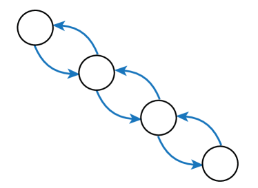
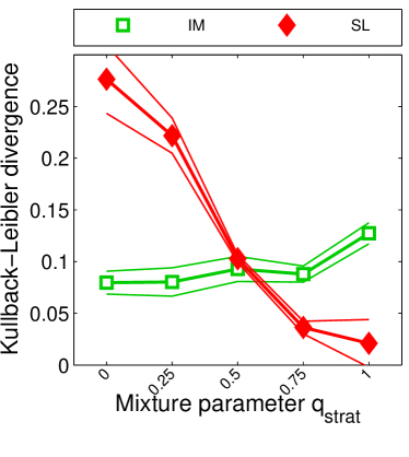
For reasons briefly discussed at the end of Section 2.1, we have little interest in determining how much worst game-theoretic models are relative to probabilistic models when applied to data from purely probabilistic processes, without any strategic component, as we think this to be a futile exercise. We believe the same is true for evaluating the quality of a probabilistic graphical model vs. a game-theoretic model when applied to strategic behavioral data, resulting from a process defined by game-theoretic concepts based on the (stable) outcomes of a game. Nevertheless, we summarize some experiments in Figure 3 that should help illustrate the point of discussed at the end of Section 2.1.
Still, for scientific curiosity, we compare LIGs to learning Ising models. Once again, our goal is not to show the superiority of either games or Ising models. For players, we perform exact -regularized maximum likelihood estimation by using the FOBOS algorithm [Duchi and Singer, 2009a, b] and exact gradients of the log-likelihood of the Ising model. Since the computation of the exact gradient at each step is NP-hard, we used this method only for . For players, we use the Höfling-Tibshirani method [Höfling and Tibshirani, 2009], which uses a sequence of first-order approximations of the exact log-likelihood. We also used a two-step algorithm, by first learning the structure by -regularized logistic regression [Wainwright et al., 2007] and then using the FOBOS algorithm [Duchi and Singer, 2009a, b] with belief propagation for gradient approximation. We did not find a statistically significant difference between the test log-likelihood of both algorithms and therefore we only report the latter.
Our experimental setup is as follows: after learning a model for different values of the regularization parameter in a training set, we select the value of that maximizes the log-likelihood in a validation set, and report statistics in a test set. For synthetic experiments, we report the Kullback-Leibler (KL) divergence, average precision (one minus the fraction of falsely included equilibria), average recall (one minus the fraction of falsely excluded equilibria) in order to measure the closeness of the recovered models to the ground truth. For real-world experiments, we report the log-likelihood. In both synthetic and real-world experiments, we report the number of equilibria and the empirical proportion of equilibria. Our results are statistically significant, we avoided showing error bars for clarity of presentation since error bars and markers overlapped.
8.1 Experiments on Synthetic Data

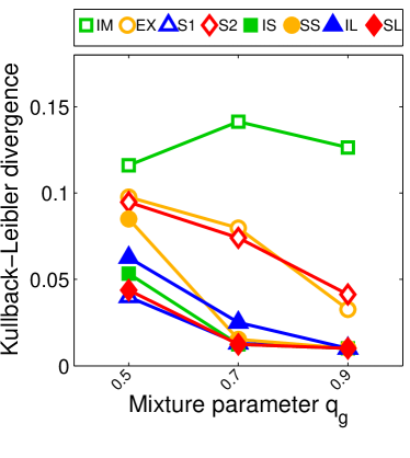
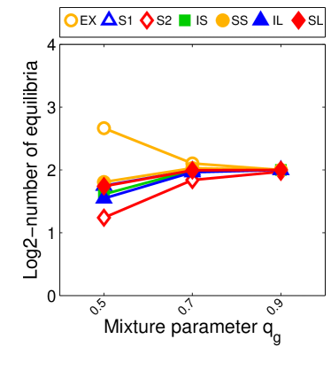 First synthetic model
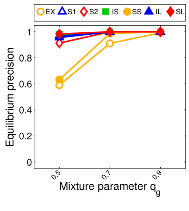
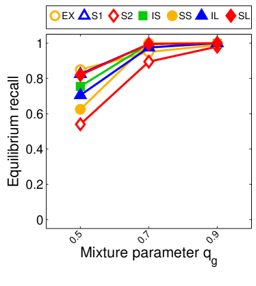
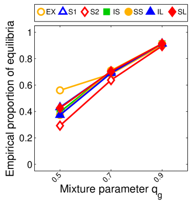
We first test the ability of the proposed methods to recover the PSNE induced by ground-truth games from data when those games are LIGs. We use a small first synthetic model in order to compare with the (super-exponential) exhaustive search method. The ground-truth model has players and 4 Nash equilibria (i.e., =0.25), was set according to Figure 4 (the weight of each edge was set to ) and . The mixture parameter of the ground-truth model was set to 0.5,0.7,0.9. For each of 50 repetitions, we generated a training, a validation and a test set of 50 samples each. Figure 4 shows that our convex loss methods and sigmoidal maximum likelihood outperform (lower KL) exhaustive search, sigmoidal maximum empirical proportion of equilibria and Ising models. Note that the exhaustive search method which performs exact maximum likelihood suffers from over-fitting and consequently does not produce the lowest KL. From all convex loss methods, simultaneous logistic regression achieves the lowest KL. For all methods, the recovery of equilibria is perfect for (number of equilibria equal to the ground truth, equilibrium precision and recall equal to 1). Additionally, the empirical proportion of equilibria resembles the mixture parameter of the ground-truth model .
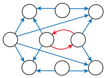
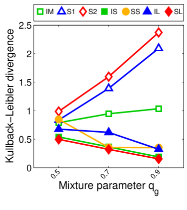
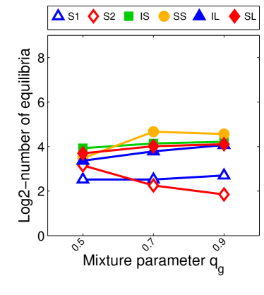 Second synthetic model
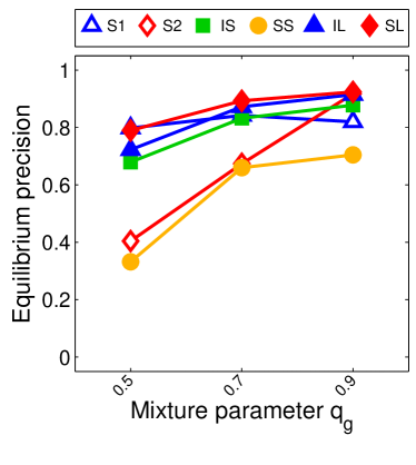
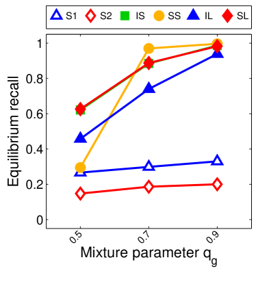
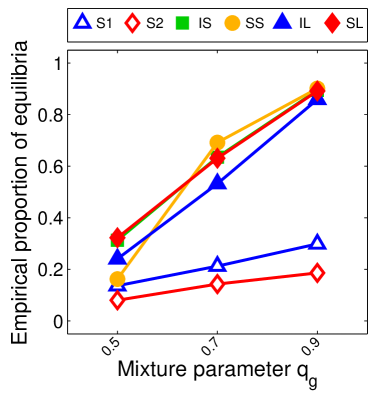
Next, we use a slightly larger second synthetic model with more complex interactions. We still keep the model small enough in order to compare with the (NP-hard) sigmoidal maximum likelihood method. The ground truth model has players and 16 Nash equilibria (i.e., =0.03125), was set according to Figure 5 (the weight of each blue and red edge was set to and respectively) and . The mixture parameter of the ground truth was set to 0.5,0.7,0.9. For each of 50 repetitions, we generated a training, a validation and a test set of 50 samples each. Figure 5 shows that our convex loss methods outperform (lower KL) sigmoidal methods and Ising models. From all convex loss methods, simultaneous logistic regression achieves the lowest KL. For convex loss methods, the equilibrium recovery is better than the remaining methods (number of equilibria equal to the ground truth, higher equilibrium precision and recall). Additionally, the empirical proportion of equilibria resembles the mixture parameter of the ground truth .
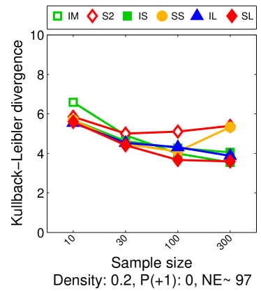
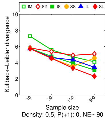
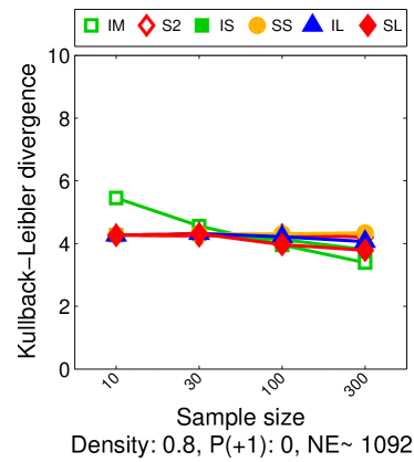
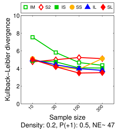
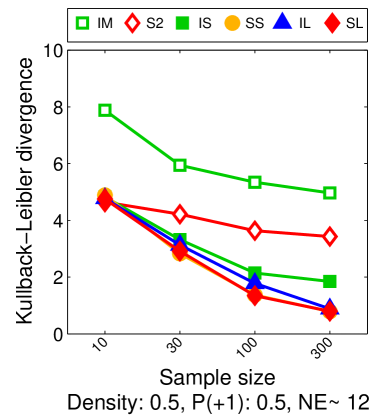
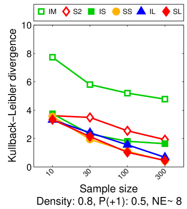
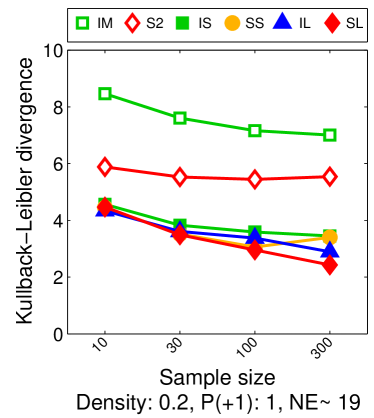
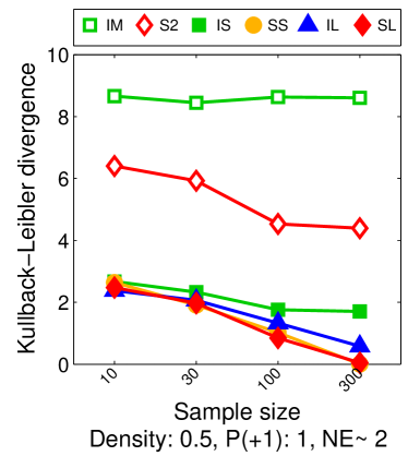
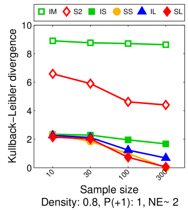
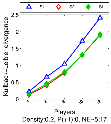
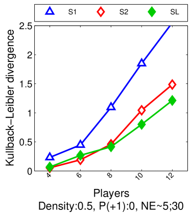
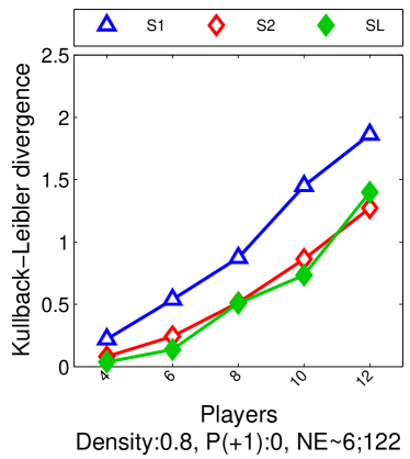
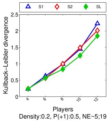
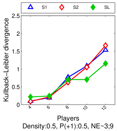
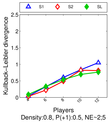
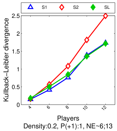
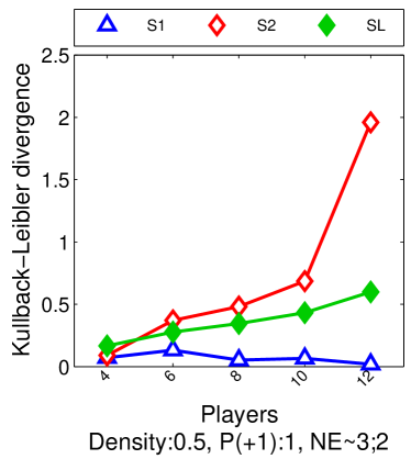
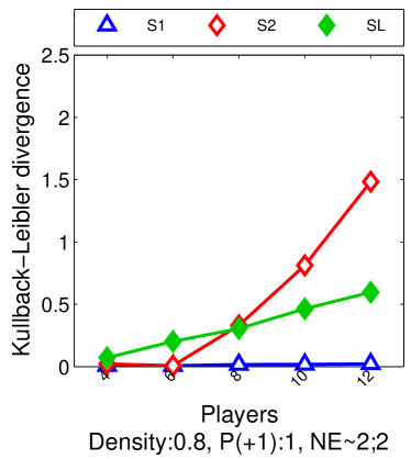
In the next experiment, we show that the performance of convex loss minimization improves as the number of samples increases. We used random graphs with slightly more variables and varying number of samples (10,30,100,300). The ground truth model contains players. For each of 20 repetitions, we generate edges in the ground truth model with a required density (either 0.2,0.5,0.8). For simplicity, the weight of each edge is set to with probability and to with probability .353535Part of the reason for using such “simple”/”limited” binary set of weight values in this synthetic experiment regards the ability to generate “interesting” LIGs; that is, games with interesting sets of PSNE. As a word of caution, this is not as simple as it appears at first glance. LIGs with weights and biases generated uniformly at random from some set of real values are almost always not interesting, often having only 1 or 2 PSNE [Irfan and Ortiz, 2014]. It is not until we move to more “special”/restricted classes of games, such as that used in this experiments, that more interesting PSNE structure arises from randomly generated LIGs. That is in large part why we concentrated our experiments in games with those simple properties. (Simplicity itself also had a role in our decision, of course.) Please understand that we are not saying that LIGs that use a larger set of integers, or non-integer real-valued weights ’s or ’s are not interesting, as the LIGs we learn from the real-world data demonstrate. What we are saying is that we do not yet have a good understanding on how to randomly generate “interesting” synthetic games from the standpoint of their induced PSNE. We leave a comprehensive evaluation of our MLE-based algorithms’ ability to recover the PSNE of randomly generated synthetic LIGs, which would involve a diversity of synthetic game graph structures, influence weights and biases that induce “interesting” sets of PSNE, for future work. Hence, the Nash equilibria of the generated games does not depend on the magnitude of the weights, just on their sign. We set the bias and the mixture parameter of the ground truth . We then generated a training and a validation set with the same number of samples. Figure 6 shows that our convex loss methods outperform (lower KL) sigmoidal maximum empirical proportion of equilibria and Ising models (except for the synthetic model with high true proportion of equilibria: density 0.8, , NE). The results are remarkably better when the number of equilibria in the ground truth model is small (e.g., for NE). From all convex loss methods, simultaneous logistic regression achieves the lowest KL.
In the next experiment, we evaluate two effects in our approximation methods. First, we evaluate the impact of removing the true proportion of equilibria from our objective function, i.e., the use of maximum empirical proportion of equilibria instead of maximum likelihood. Second, we evaluate the impact of using convex losses instead of a sigmoidal approximation of the 0/1 loss. We used random graphs with varying number of players and 50 samples. The ground truth model contains players. For each of 20 repetitions, we generate edges in the ground truth model with a required density (either 0.2,0.5,0.8). As in the previous experiment, the weight of each edge is set to with probability and to with probability . We set the bias and the mixture parameter of the ground truth . We then generated a training and a validation set with the same number of samples. Figure 7 shows that in general, convex loss methods outperform (lower KL) sigmoidal maximum empirical proportion of equilibria, and the latter one outperforms sigmoidal maximum likelihood. A different effect is observed for mild (0.5) to high (0.8) density and in which the sigmoidal maximum likelihood obtains the lowest KL. In a closer inspection, we found that the ground truth games usually have only 2 equilibria: and , which seems to present a challenge for convex loss methods. It seems that for these specific cases, removing the true proportion of equilibria from the objective function negatively impacts the estimation process, but note that sigmoidal maximum likelihood is not computationally feasible for .
8.2 Experiments on Real-World Data: U.S. Congressional Voting Records
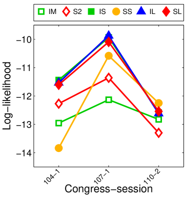
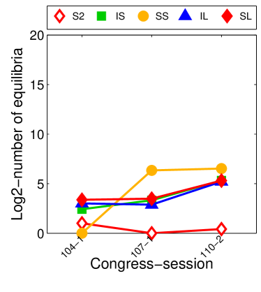
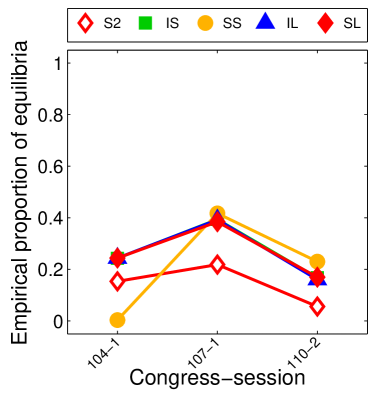
(a)
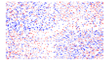
(b)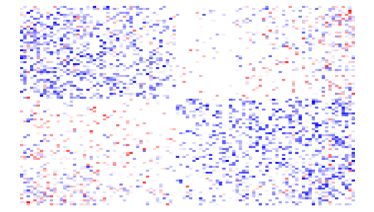

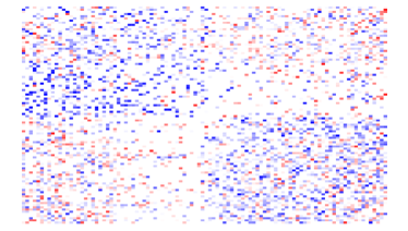
(c)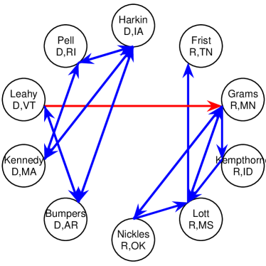
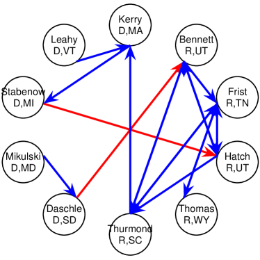
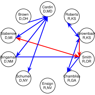
(d)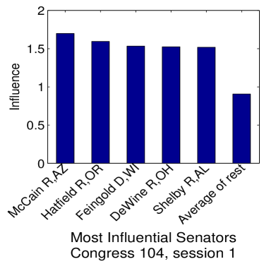
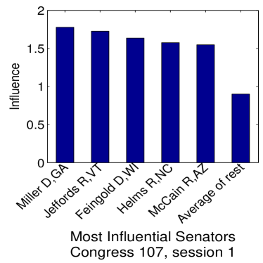
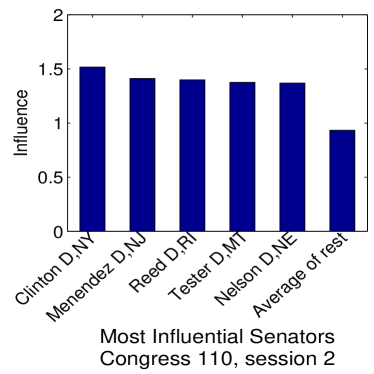
(e)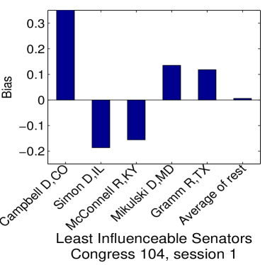
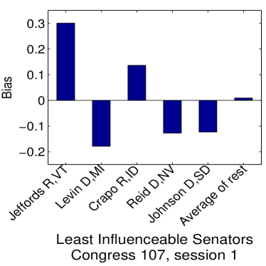
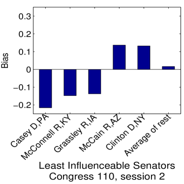
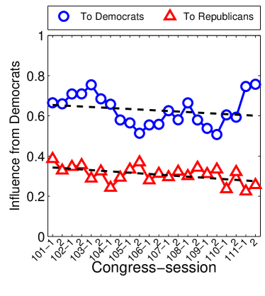
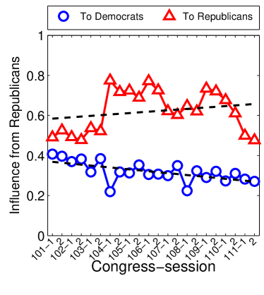
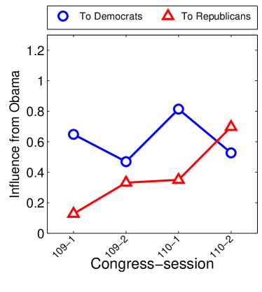
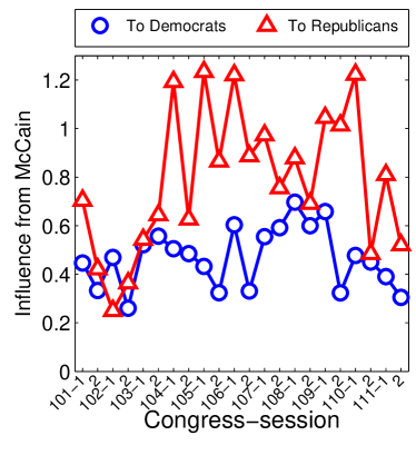
We used the U.S. congressional voting records in order to measure the generalization performance of convex loss minimization in a real-world data set. The data set is publicly available at http://www.senate.gov/. We used the first session of the 104th congress (Jan 1995 to Jan 1996, 613 votes), the first session of the 107th congress (Jan 2001 to Dec 2001, 380 votes) and the second session of the 110th congress (Jan 2008 to Jan 2009, 215 votes). Following on other researchers who have experimented with this data set (e.g., Banerjee et al. 2008), abstentions were replaced with negative votes. Since reporting the log-likelihood requires computing the number of equilibria (which is NP-hard), we selected only 20 senators by stratified random sampling. We randomly split the data into three parts. We performed six repetitions by making each third of the data take turns as training, validation and testing sets. Figure 8 shows that our convex loss methods outperform (higher log-likelihood) sigmoidal maximum empirical proportion of equilibria and Ising models. From all convex loss methods, simultaneous logistic regression achieves the lowest KL. For all methods, the number of equilibria (and so the true proportion of equilibria) is low.
We apply convex loss minimization to larger problems, by learning structures of games from all 100 senators. Figure 9 shows that simultaneous logistic regression produce structures that are sparser than its independent counterpart. The simultaneous method better elicits the bipartisan structure of the congress. We define the (aggregate) direct influence of player to all other players as after normalizing all weights, i.e., for each player we divide by . Note that Jeffords and Clinton are one of the 5 most directly-influential as well as 5 least directly-influenceable (high bias) senators, in the 107th and 110th congress respectively. McCain and Feingold are both in the list of 5 most directly-influential senators in the 104th and 107th congress. McCain appears again in the list of 5 least directly influenceable senators in the 110th congress (as defined above in the context of the LIG model).
We test the hypothesis that the aggregate direct influence, as defined by our model, between senators of the same party are stronger than senators of different party. We learn structures of games from all 100 senators from the 101th congress to the 111th congress (Jan 1989 to Dec 2010). The number of votes cast for each session were average: 337, minimum: 215, maximum: 613. Figure 10 validates our hypothesis and more interestingly, it shows that influence between different parties is decreasing over time. Note that the influence from Obama to Republicans increased in the last sessions, while McCain’s influence to Republicans decreased.
Since the U.S. Congressional voting data is observational, we used the log-likelihood as an adequate measure of predictive performance. We argue that the log-likelihood of joint actions provides a more “global view” compared to predicting the action of a single agent. Furthermore, predicting the action of a single agent (i.e., ) works under the assumption that we have access to the decisions of the other agents (i.e., ), which is in contrast to our framework. Regarding causal strategic inference, Irfan and Ortiz [2014] use the games that we produce in this section in order to address problems such as the identification of most influential senators. (We refer the reader to their paper for further details.)
9 Concluding Remarks
In Section 6, we present a variety of algorithms to learn LIGs from strictly behavioral data, including what we call independent logistic regression (ILR). There is a very popular technique for learning Ising models that uses independent regularized logistic regression to compute the individual conditional probabilities as a step toward computing a globally coherent joint probability distribution. However, this approach is inherently problematic, as some authors have previously pointed out (see, e.g., Guo et al. 2010). Without getting too technical, the main roadblock is that there is no guarantee that estimates of the weights produced by the individual regressions be symmetric: for all . Learning an Ising model requires the enforcement of this condition, and a variety of heuristics have been proposed. (Please see Section 2.1 for relevant work and references in this area.)
We also apply ILR in exactly the same manner but for a different objective: learning LIGs. Some seem to think that this diminishes the significance of our contributions. We strongly believe the opposite is true: That we can learn games by using such simple, practical, efficient and well-studied techniques is a significant plus in our view. Again, without getting too technical, the estimates of ILR need not be symmetric for LIG models, and are always perfectly consistent with the LIG definition. In fact, asymmetric estimates are common in practice (the LIG for the 110th Congress depicted in Figure 1 is an example). And we believe this makes the model more interesting. In the ILR-learned LIG, a player may have a positive, negative or no direct effect on another players utility, and vice versa.363636It is easy to come up with examples of such opposing/antagonistic interactions between individuals in real-world settings. (See, e.g., “parents with teenagers,” perhaps a more timely example is the U.S. Congress in recent times.)
Thus, despite the process of estimation of model parameters being similar, the view of the output of that estimation process is radically different in each case. Our experiments show that our generative model with LIGs built from ILR estimates achieves higher generalization likelihoods than standard probabilistic models such as Ising models that may also use ILR. This fact, that the generative model defined in terms of game-theoretic equilibrium concepts can explain the data better than traditional probabilistic models, provides further evidence supporting such a game-theoretic “view” of the ILR estimated parameters and yields additional confidence in their use in game-theoretic models.
In short, ILR is a thoroughly studied method with a long tradition and an extensive literature from which we can only benefit. We find it to a be a good, unexpected outcome of our research in this work, and thus a reasonably significant contribution, that we can successfully and effectively use ILR, a very simple and practical estimation technique for learning probabilistic graphical models, to learn game-theoretic graphical models too.
9.1 Extensions and Future Work
There are several ways of extending this research. We can extend our approach to -approximate PSNE.373737By definition, given , a joint pure-strategy is an -approximate PSNE if for each player , we have ; in other words, no players can gain more than in payoff/utility value from unilaterally deviating from , assuming the other players play . Using this definition, we can see that a PSNE is simply a -approximate PSNE. In this case, for each player instead of one condition, we will have two best-response conditions which are still linear in and . Additionally, we can extend our approach to a broader class of graphical games and non-Boolean actions. Note that our analysis does not rely on binary actions, but on binary features of one player or two players . We can use features of three players or of non-Boolean actions . This kernelized version is still linear in and . These extensions are possible because our algorithms and analysis rely on linearity and binary features; additionally, we can obtain a new upper-bound on the “VC-dimension” by changing the inputs of the neural-network architecture. We can easily extend our approach to parameter learning for fixed structures by using a regularizer instead.
Future work should also consider and study more sophisticated noise processes, MSNE, and the analysis of different upper bounds for the 0/1 loss (e.g., exponential, smooth hinge). Finally, we should consider other slightly more complex versions of our model based on Bayesian or stochastic games to account for possible variations of the influence-weights and bias-threshold parameters. As an example, we may consider versions of our model for congressional voting that would explicitly capture game differences in terms of influences and biases that depend on the nature or topic of each specific bill being voted on, as well as Senators’ time-changing preferences and trends.
Acknowledgements
We are grateful to Christian Luhmann for extensive discussion of many aspects of this work and the multiple comments and feedback he provided to improve both the work and the presentation. We warmly thank Tommi Jaakkola for several informal discussions on the topic of learning games and the ideas behind causal strategic inference, as well as suggestions on how to improve the presentation. We also thank Mohammad Irfan for his help with motivating causal strategic inference in inference games and examples to illustrate their use. We would also like to thank Alexander Berg, Tamara Berg and Dimitris Samaras for their comments and questions during informal presentations of this work, which helped us tailor the presentation to a wider audience. We are very grateful to Nicolle Gruzling for sharing her Master’s thesis [Gruzling, 2006] which contains valuable references used in Section 6.2. Finally, we thank several anonymous reviewers for their comments and feedback, and in particular, an anonymous reviewer for the reference to an overview on the literature on composite marginal likelihoods.
Shorter versions of the work presented here appear as Chapter 7 of the first author’s Ph.D. dissertation [Honorio, 2012] and as e-print arXiv:1206.3713 [cs.LG] [Honorio and Ortiz, 2012].
This work was supported in part by NSF CAREER Award IIS-1054541.
Appendix A Additional Discussion
In this section, we discuss our choice of modeling end-state predictions without modeling dynamics. We also discuss some alternative noise models to the one studied in this manuscript.
A.1 On End-State Predictions without Explicitly Modeling Dynamics
Certainly, in cases in which information about the dynamics is available, the learned model may use such information while still making end-state predictions. But no such information, either via data sequences or prior knowledge, is available in any of the publicly-available real-world data sets we study here. Take congressional voting as an example. Considering the voting records as sequence of votes does not seem sensible in our context from a modeling/engineering perspective because the data set does not have any detailed information about the nature of the vote: we just have each senator’s vote on whatever bill they considered, and little to no information about the detailed dynamics that might have lead to the senators’ final votes. Indeed, one may go further and argue that assuming the the availability of information about the dynamics of the process is a considerable burden on the modeler and something of a wishful thinking in many practical, real-world settings.
Besides the nature of our setting, the lack of data or information, and the CSI motivation, there are other more fundamental ML reasons why we have no interest in considering dynamics in this paper. First, we view the additional complexity of a dynamic/temporal model as providing the wrong tradeoff: dynamic/temporal models are often inherently more complex to express and learn from data. Second, it is common ML practice to separate single example/outcome problems from sequence problems; said differently, ML generally treats the problem of learning from individual i.i.d. examples different from that of learning from sequences or sequence prediction. Third, we invoke Vapnik’s Principle of Transduction (Vapnik, 1998, page 477):383838See also http://www.cs.man.ac.uk/~jknowles/transductive.html additional information.
“When solving a problem of interest, do not solve a more general problem as an intermediate step. Try to get the answer that you really need but not a more general one.”
We believe this additional complexity of temporal dynamics, while possibly more “realistic,” might easily weaken the power of the “bottom-line” prediction of the possible stable final outcomes because the resulting models can get side-tracked by the details of the interaction. We believe the difficulty of modeling such details, specially with the relatively limited amount of the data available, leads to poor prediction performance on what we really care about from an engineering stand point: We would like to know or predict what will end up happening, and have little or no interest on the how or why this happens.
We recognize the scientific significance and importance of research in social and behavioral sciences such as sociology, psychology and, in some cases economics, on explaining, at a higher level of abstraction, often going as low as the “cognitive” or “neuroscience” level, the process by which final decisions are reached.
We believe the sudden growth of interest from industry (both online and physical companies), government and other national and international institutions on predicting “behavior” for the purpose of revenue, improving efficiency, instituting effective policies with minimal regulations, etc., should shift the focus of the study of “behavior” closer to an engineering endeavor. We believe such entities are after the “bottom line” and will care more about the end-goal than how or why a specific outcome is achieved, modulo, of course, having simple enough and tractable computational models that provide reasonably accurate predictions of final end-state behavior, or at least accurate enough for their purposes.
A.2 On Alternative Noise Models
Next, we discuss some alternative noise models to the one studied in this manuscript. Specifically, we discuss an extension of the PSNE-based mixture noise model as well as individual-player noise models.
A.2.1 On Generalizations of the PSNE-based Mixture Noise Models
A simple extension to our model in Eq. (1) is to allow for more general distributions for the PSNE and the non-PSNE sets. That is, with some probability , a joint action is chosen from by following a distribution parameterized by ; otherwise, is chosen from its complement set by following a distribution parameterized by . The corresponding probability mass function (PMF) over joint-behaviors parameterized by is
where is a game, and are PMFs over .
One reasonable technique to learn such a model from data is to perform an alternate method. Compared to our simpler model, this model requires a step that maximizes the likelihood by changing and while keeping and constant. The complexity of this step will depend on how we parameterize the PMFs and but will very likely be an NP-hard problem because of the partition function. Furthermore, the problem of maximizing the likelihood by changing (while keeping , and constant) is combinatorial in nature and in this paper, we provided a tractable approximation method with provable guarantees (for the case of uniform distributions). Other approaches for maximizing the likelihood by changing are very likely to be exponential as we discuss briefly at the start of Section 6.
A.2.2 On Individual-Player Noise Models
As an example, consider a the generative model in which we first randomly select a PSNE of the game from a distribution parameterized by , and then each player , independently, acts according to with probability and switches its action with probability . The corresponding probability mass function (PMF) over joint-behaviors parameterized by is
where is a game, and is a PMF over .
One reasonable technique to learn such a model from data is to perform an alternate method. In one step, we maximize the likelihood by changing while keeping and constant, which could be tractably performed by applying Jensen’s inequality since the problem is combinatorial in nature. In another step, we maximize the likelihood by changing while keeping and constant, which could be performed by gradient ascent (the complexity of this step depends on the size of which could be exponential!). In yet another step, we maximize the likelihood by changing while keeping and constant (the complexity of this step will depend on how we parameterize the PMF but will very likely be an NP-hard problem because of the partition function). The main problem with this technique is that it can be formally proved that the first step (Jensen’s inequality) will almost surely pick a single equilibria for the model (i.e., ).
References
- Ackermann and Skopalik [2007] H. Ackermann and A. Skopalik. On the Complexity of Pure Nash Equilibria in Player-Specific Network Congestion Games. In X. Deng and F. Graham, editors, Internet and Network Economics, volume 4858 of Lecture Notes in Computer Science, pages 419–430. Springer Berlin Heidelberg, 2007.
- Aichholzer and Aurenhammer [1996] O. Aichholzer and F. Aurenhammer. Classifying Hyperplanes in Hypercubes. SIAM Journal on Discrete Mathematics, 9(2):225–232, 1996.
- Aumann [1974] R. Aumann. Subjectivity and Correlation in Randomized Strategies. Journal of Mathematical Economics, 1:67–96, 1974.
- Ballester et al. [2004] C. Ballester, A. Calvó-Armengol, and Y. Zenou. Who’s Who in Crime Networks. Wanted: the Key Player. Working Paper Series 617, Research Institute of Industrial Economics, 2004.
- Ballester et al. [2006] C. Ballester, A. Calvó-Armengol, and Y. Zenou. Who’s Who in Networks. Wanted: The Key Player. Econometrica, 74(5):1403–1417, 2006.
- Banerjee et al. [2008] O. Banerjee, L. El Ghaoui, and A. d’Aspremont. Model Selection Through Sparse Maximum Likelihood Estimation for Multivariate Gaussian or Binary Data. Journal of Machine Learning Research, 9:485–516, 2008.
- Banerjee et al. [2006] O. Banerjee, L. El Ghaoui, A. d’Aspremont, and G. Natsoulis. Convex Optimization Techniques for Fitting Sparse Gaussian Graphical Models. In W. Cohen and A. Moore, editors, Proceedings of the 23nd International Machine Learning Conference, pages 89–96. Omni Press, 2006.
- Blum et al. [2006] B. Blum, C.R. Shelton, and D. Koller. A Continuation Method for Nash Equilibria in Structured Games. Journal of Artificial Intelligence Research, 25:457–502, 2006.
- Boyd and Vandenberghe [2006] S. Boyd and L. Vandenberghe. Convex Optimization. Cambridge University Press, 2006.
- Bradley and Mangasarian [1998] P. S. Bradley and O. L. Mangasarian. Feature Selection via Concave Minimization and Support Vector Machines. In Proceedings of the 15th International Conference on Machine Learning, ICML ’98, pages 82–90, San Francisco, CA, USA, 1998. Morgan Kaufmann Publishers Inc.
- Brock and Durlauf [2001] W. Brock and S. Durlauf. Discrete Choice with Social Interactions. The Review of Economic Studies, 68(2):235–260, 2001.
- Camerer [2003] C. Camerer. Behavioral Game Theory: Experiments on Strategic Interaction. Princeton University Press, 2003.
- Cao et al. [2011] T. Cao, X. Wu, T. Hu, and S. Wang. Active Learning of Model Parameters for Influence Maximization. In D. Gunopulos, T. Hofmann, D. Malerba, and M. Vazirgiannis, editors, Machine Learning and Knowledge Discovery in Databases, volume 6911 of Lecture Notes in Computer Science, pages 280–295. Springer Berlin Heidelberg, 2011.
- Chapman et al. [2010] A. Chapman, A. Farinelli, E. Munoz de Cote, A. Rogers, and N. Jennings. A Distributed Algorithm for Optimising over Pure Strategy Nash Equilibria. In AAAI Conference on Artificial Intelligence, 2010.
- Chickering [2002] D. Chickering. Learning Equivalence Classes of Bayesian-Network Structures. Journal of Machine Learning Research, 2:445–498, 2002.
- Chow and Liu [1968] C. Chow and C. Liu. Approximating Discrete Probability Distributions with Dependence Trees. IEEE Transactions on Information Theory, 14(3):462–467, 1968.
- Daskalakis et al. [2011] C. Daskalakis, A. Dimakisy, and E. Mossel. Connectivity and Equilibrium in Random Games. Annals of Applied Probability, 21(3):987–1016, 2011.
- Daskalakis et al. [2009] C. Daskalakis, P. Goldberg, and C. Papadimitriou. The complexity of computing a Nash equilibrium. Communications of the ACM, 52(2):89–97, 2009.
- Daskalakis and Papadimitriou [2006] C. Daskalakis and C.H. Papadimitriou. Computing Pure Nash Equilibria in Graphical Games via Markov Random Fields. In Proceedings of the 7th ACM Conference on Electronic Commerce, EC ’06, pages 91–99, New York, NY, USA, 2006. ACM.
- Dilkina et al. [2007] B. Dilkina, C. P. Gomes, and A. Sabharwal. The Impact of Network Topology on Pure Nash Equilibria in Graphical Games. In Proceedings of the 22nd National Conference on Artificial Intelligence - Volume 1, AAAI’07, pages 42–49. AAAI Press, 2007.
- Domingos [2005] P. Domingos. Mining Social Networks for Viral Marketing. IEEE Intelligent Systems, 20(1):80–82, 2005. Short Paper.
- Domingos and Richardson [2001] P. Domingos and M. Richardson. Mining the Network Value of Customers. In Proceedings of the 7th ACM SIGKDD International Conference on Knowledge Discovery and Data Mining, KDD ’01, pages 57–66, New York, NY, USA, 2001. ACM.
- Duchi and Singer [2009a] J. Duchi and Y. Singer. Efficient Learning using Forward-Backward Splitting. In Y. Bengio, D. Schuurmans, J.D. Lafferty, C.K.I. Williams, and A. Culotta, editors, Advances in Neural Information Processing Systems 22, pages 495–503. Curran Associates, Inc., 2009a.
- Duchi and Singer [2009b] J. Duchi and Y. Singer. Efficient Online and Batch Learning using Forward Backward Splitting. Journal of Machine Learning Research, 10:2899–2934, 2009b.
- Dunkel [2007] J. Dunkel. Complexity of Pure-Strategy Nash Equilibria in Non-Cooperative Games. In K.-H. Waldmann and U. M. Stocker, editors, Operations Research Proceedings, volume 2006, pages 45–51. Springer Berlin Heidelberg, 2007.
- Dunkel and Schulz [2006] J. Dunkel and A. Schulz. On the Complexity of Pure-Strategy Nash Equilibria in Congestion and Local-Effect Games. In P. Spirakis, M. Mavronicolas, and S. Kontogiannis, editors, Internet and Network Economics, volume 4286 of Lecture Notes in Computer Science, pages 62–73. Springer Berlin Heidelberg, 2006.
- Duong et al. [2009] Q. Duong, Y. Vorobeychik, S. Singh, and M.P. Wellman. Learning Graphical Game Models. In Proceedings of the 21st International Joint Conference on Artificial Intelligence, IJCAI’09, pages 116–121, San Francisco, CA, USA, 2009. Morgan Kaufmann Publishers Inc.
- Duong et al. [2008] Q. Duong, M. Wellman, and S. Singh. Knowledge Combination in Graphical Multiagent Model. In Proceedings of the 24th Annual Conference on Uncertainty in Artificial Intelligence (UAI-08), pages 145–152, Corvallis, Oregon, 2008. AUAI Press.
- Duong et al. [2012] Q. Duong, M.P. Wellman, S. Singh, and M. Kearns. Learning and Predicting Dynamic Networked Behavior with Graphical Multiagent Models. In Proceedings of the 11th International Conference on Autonomous Agents and Multiagent Systems - Volume 1, AAMAS ’12, pages 441–448, Richland, SC, 2012. International Foundation for Autonomous Agents and Multiagent Systems.
- Duong et al. [2010] Q. Duong, M.P. Wellman, S. Singh, and Y. Vorobeychik. History-dependent Graphical Multiagent Models. In Proceedings of the 9th International Conference on Autonomous Agents and Multiagent Systems: Volume 1, AAMAS ’10, pages 1215–1222, Richland, SC, 2010. International Foundation for Autonomous Agents and Multiagent Systems.
- Even-Dar and Shapira [2007] E. Even-Dar and A. Shapira. A Note on Maximizing the Spread of Influence in Social Networks. In X. Deng and F. Graham, editors, Internet and Network Economics, volume 4858 of Lecture Notes in Computer Science, pages 281–286. Springer Berlin Heidelberg, 2007.
- Fabrikant et al. [2004] A. Fabrikant, C. Papadimitriou, and K. Talwar. The Complexity of Pure Nash Equilibria. In Proceedings of the 36th Annual ACM Symposium on Theory of Computing, STOC ’04, pages 604–612, New York, NY, USA, 2004. ACM.
- Ficici et al. [2008] S. Ficici, D. Parkes, and A. Pfeffer. Learning and Solving Many-Player Games through a Cluster-Based Representation. In Proceedings of the 24th Annual Conference on Uncertainty in Artificial Intelligence (UAI-08), pages 188–195, Corvallis, Oregon, 2008. AUAI Press.
- Fudenberg and Levine [1999] D. Fudenberg and D. Levine. The Theory of Learning in Games. MIT Press, 1999.
- Fudenberg and Tirole [1991] D. Fudenberg and J. Tirole. Game Theory. The MIT Press, 1991.
- Gao and Pfeffer [2010] X. Gao and A. Pfeffer. Learning Game Representations from Data Using Rationality Constraints. In Proceedings of the 26th Annual Conference on Uncertainty in Artificial Intelligence (UAI-10), pages 185–192, Corvallis, Oregon, 2010. AUAI Press.
- Gilboa and Zemel [1989] I. Gilboa and E. Zemel. Nash and correlated equilibria: some complexity considerations. Games and Economic Behavior, 1(1):80–93, 1989.
- Gomez Rodriguez et al. [2010] M. Gomez Rodriguez, J. Leskovec, and A. Krause. Inferring Networks of Diffusion and Influence. In Proceedings of the 16th ACM SIGKDD International Conference on Knowledge Discovery and Data Mining, KDD ’10, pages 1019–1028, New York, NY, USA, 2010. ACM.
- Gottlob et al. [2005] G. Gottlob, G. Greco, and F. Scarcello. Pure Nash equilibria: Hard and easy games. Journal of Artificial Intelligence Research, 24(1):357–406, 2005.
- Goyal et al. [2010] A. Goyal, F. Bonchi, and L.V.S. Lakshmanan. Learning Influence Probabilities in Social Networks. In Proceedings of the 3rd ACM International Conference on Web Search and Data Mining, WSDM ’10, pages 241–250, New York, NY, USA, 2010. ACM.
- Granovetter [1978] M. Granovetter. Threshold Models of Collective Behavior. The American Journal of Sociology, 83(6):1420–1443, 1978.
- Gruzling [2006] N. Gruzling. Linear Separability of the Vertices of an -Dimensional Hypercube. Master’s thesis, The University of British Columbia, 2006.
- Guo et al. [2010] J. Guo, E. Levina, G. Michailidis, and J. Zhu. Joint structure estimation for categorical Markov networks. Technical report, University of Michigan, Department of Statistics, 2010. Submitted. http://www.stat.lsa.umich.edu/~elevina.
- Guo and Schuurmans [2006] Y. Guo and D. Schuurmans. Convex Structure Learning for Bayesian Networks: Polynomial Feature Selection and Approximate Ordering. In Proceedings of the 22nd Annual Conference on Uncertainty in Artificial Intelligence (UAI-06), pages 208–216, Arlington, Virginia, 2006. AUAI Press.
- Hasan and Galiana [2008] E. Hasan and F. Galiana. Electricity Markets Cleared by Merit Order–Part II: Strategic Offers and Market Power. IEEE Transactions on Power Systems, 23(2):372–379, 2008.
- Hasan and Galiana [2010] E. Hasan and F. Galiana. Fast Computation of Pure Strategy Nash Equilibria in Electricity Markets Cleared by Merit Order. IEEE Transactions on Power Systems, 25(2):722–728, 2010.
- Hasan et al. [2008] E. Hasan, F. Galiana, and A. Conejo. Electricity Markets Cleared by Merit Order–Part I: Finding the Market Outcomes Supported by Pure Strategy Nash Equilibria. IEEE Transactions on Power Systems, 23(2):361–371, 2008.
- Heal and Kunreuther [2003] G. Heal and H. Kunreuther. You Only Die Once: Managing Discrete Interdependent Risks. Working Paper W9885, National Bureau of Economic Research, 2003.
- Heal and Kunreuther [2006] G. Heal and H. Kunreuther. Supermodularity and Tipping. Working Paper 12281, National Bureau of Economic Research, 2006.
- Heal and Kunreuther [2007] G. Heal and H. Kunreuther. Modeling Interdependent Risks. Risk Analysis, 27:621–634, 2007.
- Höfling and Tibshirani [2009] H. Höfling and R. Tibshirani. Estimation of Sparse Binary Pairwise Markov Networks using Pseudo-likelihoods. Journal of Machine Learning Research, 10:883–906, 2009.
- Honorio [2012] J. Honorio. Tractable Learning of Graphical Model Structures from Data. PhD thesis, Stony Brook University, Department of Computer Science, 2012.
- Honorio and Ortiz [2012] J. Honorio and L. Ortiz. Learning the Structure and Parameters of Large-Population Graphical Games from Behavioral Data. Computer Research Repository, 2012. http://arxiv.org/abs/1206.3713.
- Irfan and Ortiz [2014] M. Irfan and L. E. Ortiz. On Influence, Stable Behavior, and the Most Influential Individuals in Networks: A Game-Theoretic Approach. Artificial Intelligence, 215:79–119, 2014.
- Janovskaja [1968] E. Janovskaja. Equilibrium situations in multi-matrix games. Litovskiĭ Matematicheskiĭ Sbornik, 8:381–384, 1968.
- Jiang and Leyton-Brown [2008] A. Jiang and K. Leyton-Brown. Action-Graph Games. Technical Report TR-2008-13, University of British Columbia, Department of Computer Science, 2008.
- Jiang and Leyton-Brown [2011] A.X. Jiang and K. Leyton-Brown. Polynomial-time Computation of Exact Correlated Equilibrium in Compact Games. In Proceedings of the 12th ACM Conference on Electronic Commerce, EC ’11, pages 119–126, New York, NY, USA, 2011. ACM.
- Kakade et al. [2003] S. Kakade, M. Kearns, J. Langford, and L. Ortiz. Correlated Equilibria in Graphical Games. In Proceedings of the 4th ACM Conference on Electronic Commerce, EC ’03, pages 42–47, New York, NY, USA, 2003. ACM.
- Kearns [2005] M. Kearns. Economics, Computer Science, and Policy. Issues in Science and Technology, 2005.
- Kearns et al. [2001] M. Kearns, M. Littman, and S. Singh. Graphical Models for Game Theory. In Proceedings of the 17th Annual Conference on Uncertainty in Artificial Intelligence (UAI-01), pages 253–260, San Francisco, CA, 2001. Morgan Kaufmann.
- Kearns and Vazirani [1994] M. Kearns and U. Vazirani. An Introduction to Computational Learning Theory. The MIT Press, 1994.
- Kearns and Wortman [2008] M. Kearns and J. Wortman. Learning from Collective Behavior. In R.A. Servedio and T. Zhang, editors, 21st Annual Conference on Learning Theory - COLT 2008, Helsinki, Finland, July 9-12, 2008, COLT ’08, pages 99–110. Omnipress, 2008.
- Kleinberg [2007] J. Kleinberg. Cascading Behavior in Networks: Algorithmic and Economic Issues. In N. Nisan, T. Roughgarden, É. Tardos, and V. V. Vazirani, editors, Algorithmic Game Theory, chapter 24, pages 613–632. Cambridge University Press, 2007.
- Koller and Friedman [2009] D. Koller and N. Friedman. Probabilistic Graphical Models: Principles and Techniques. The MIT Press, 2009.
- Koller and Milch [2003] D. Koller and B. Milch. Multi-agent influence diagrams for representing and solving games. Games and Economic Behavior, 45(1):181–221, 2003.
- Kunreuther and Michel-Kerjan [2007] H. Kunreuther and E. Michel-Kerjan. Assessing, Managing and Benefiting from Global Interdependent Risks: The Case of Terrorism and Natural Disasters, 2007. CREATE Symposium: http://opim.wharton.upenn.edu/risk/library/AssessingRisks-2007.pdf.
- La Mura [2000] P. La Mura. Game Networks. In Proceedings of the 16th Annual Conference on Uncertainty in Artificial Intelligence (UAI-00), pages 335–342, San Francisco, CA, 2000. Morgan Kaufmann.
- Lee et al. [2007] S. Lee, V. Ganapathi, and D. Koller. Efficient Structure Learning of Markov Networks using -Regularization. In B. Schölkopf, J.C. Platt, and T. Hoffman, editors, Advances in Neural Information Processing Systems 19, pages 817–824. MIT Press, 2007.
- López-Pintado and Watts [2008] D. López-Pintado and D. Watts. Social Influence, Binary Decisions and Collective Dynamics. Rationality and Society, 20(4):399–443, 2008.
- McKelvey and Palfrey [1995] R. McKelvey and T. Palfrey. Quantal Response Equilibria for Normal Form Games. Games and Economic Behavior, 10(1):6–38, 1995.
- Morris [2000] S. Morris. Contagion. The Review of Economic Studies, 67(1):57–78, 2000.
- Muroga [1965] S. Muroga. Lower bounds on the number of threshold functions and a maximum weight. IEEE Transactions on Electronic Computers, 14:136–148, 1965.
- Muroga [1971] S. Muroga. Threshold Logic and Its Applications. John Wiley & Sons, 1971.
- Muroga and Toda [1966] S. Muroga and I. Toda. Lower Bound of the Number of Threshold Functions. IEEE Transactions on Electronic Computers, 5:805–806, 1966.
- Nash [1951] J. Nash. Non-cooperative games. Annals of Mathematics, 54(2):286–295, 1951.
- Ng and Russell [2000] A. Y. Ng and S. J. Russell. Algorithms for Inverse Reinforcement Learning. In Proceedings of the 17th International Conference on Machine Learning, ICML ’00, pages 663–670, San Francisco, CA, USA, 2000. Morgan Kaufmann Publishers Inc.
- Nisan et al. [2007] N. Nisan, T. Roughgarden, É. Tardos, and V. V. Vazirani, editors. Algorithmic Game Theory. Cambridge University Press, 2007.
- Ortiz and Kearns [2003] L. E. Ortiz and M. Kearns. Nash Propagation for Loopy Graphical Games. In S. Becker, S. Thrun, and K. Obermayer, editors, Advances in Neural Information Processing Systems 15, pages 817–824. MIT Press, 2003.
- Papadimitriou and Roughgarden [2008] C. Papadimitriou and T. Roughgarden. Computing correlated equilibria in multi-player games. Journal of the ACM, 55(3):1–29, 2008.
- Rinott and Scarsini [2000] Y. Rinott and M. Scarsini. On the Number of Pure Strategy Nash Equilibria in Random Games. Games and Economic Behavior, 33(2):274–293, 2000.
- Rosenthal [1973] R. Rosenthal. A class of games possessing pure-strategy Nash equilibria. International Journal of Game Theory, 2(1):65–67, 1973.
- Ryan et al. [2010] C.T. Ryan, A.X. Jiang, and K. Leyton-Brown. Computing Pure Strategy Nash Equilibria in Compact Symmetric Games. In Proceedings of the 11th ACM Conference on Electronic Commerce, EC ’10, pages 63–72, New York, NY, USA, 2010. ACM.
- Saito et al. [2009] K. Saito, M. Kimura, K. Ohara, and H. Motoda. Learning Continuous-Time Information Diffusion Model for Social Behavioral Data Analysis. In Z. Zhou and T. Washio, editors, Advances in Machine Learning, volume 5828 of Lecture Notes in Computer Science, pages 322–337. Springer Berlin Heidelberg, 2009.
- Saito et al. [2010] K. Saito, M. Kimura, K. Ohara, and H. Motoda. Selecting Information Diffusion Models over Social Networks for Behavioral Analysis. In J. L. Balcázar, F. Bonchi, A. Gionis, and M. Sebag, editors, Machine Learning and Knowledge Discovery in Databases, volume 6323 of Lecture Notes in Computer Science, pages 180–195. Springer Berlin Heidelberg, 2010.
- Saito et al. [2008] K. Saito, R. Nakano, and M. Kimura. Prediction of Information Diffusion Probabilities for Independent Cascade Model. In I. Lovrek, R. J. Howlett, and L. C. Jain, editors, Knowledge-Based Intelligent Information and Engineering Systems, volume 5179 of Lecture Notes in Computer Science, pages 67–75. Springer Berlin Heidelberg, 2008.
- Schmidt et al. [2007a] M. Schmidt, G. Fung, and R. Rosales. Fast Optimization Methods for L1 Regularization: A Comparative Study and Two New Approaches. In Proceedings of the 18th European Conference on Machine Learning, ECML ’07, pages 286–297, Berlin, Heidelberg, 2007a. Springer-Verlag.
- Schmidt and Murphy [2009] M. Schmidt and K. Murphy. Modeling Discrete Interventional Data using Directed Cyclic Graphical Models. In Proceedings of the 25th Annual Conference on Uncertainty in Artificial Intelligence (UAI-09), pages 487–495, Corvallis, Oregon, 2009. AUAI Press.
- Schmidt et al. [2007b] M. Schmidt, A. Niculescu-Mizil, and K. Murphy. Learning Graphical Model Structure Using -regularization Paths. In Proceedings of the 22nd National Conference on Artificial Intelligence - Volume 2, pages 1278–1283, 2007b.
- Shoham [2008] Y. Shoham. Computer Science and Game Theory. Communications of the ACM, 51(8):74–79, 2008.
- Shoham and Leyton-Brown [2009] Y. Shoham and K. Leyton-Brown. Multiagent Systems: Algorithmic, Game-Theoretic, and Logical Foundations. Cambridge University Press, 2009.
- Sontag [1998] E. Sontag. VC Dimension of Neural Networks. Neural Networks and Machine Learning, pages 69–95, 1998.
- Srebro [2001] N. Srebro. Maximum Likelihood Bounded Tree-Width Markov Networks. In Proceedings of the 17th Annual Conference on Uncertainty in Artificial Intelligence (UAI-01), pages 504–511, San Francisco, CA, 2001. Morgan Kaufmann.
- Stanford [1995] W. Stanford. A Note on the Probability of Pure Nash Equilibria in Matrix Games. Games and Economic Behavior, 9(2):238–246, 1995.
- Sureka and Wurman [2005] A. Sureka and P.R. Wurman. Using Tabu Best-response Search to Find Pure Strategy Nash Equilibria in Normal Form Games. In Proceedings of the 4th International Joint Conference on Autonomous Agents and Multiagent Systems, AAMAS ’05, pages 1023–1029, New York, NY, USA, 2005. ACM.
- Vapnik [1998] V. Vapnik. Statistical Learning Theory. Wiley, 1998.
- Vickrey and Koller [2002] D. Vickrey and D. Koller. Multi-agent Algorithms for Solving Graphical Games. In 18th National Conference on Artificial Intelligence, pages 345–351, Menlo Park, CA, USA, 2002. American Association for Artificial Intelligence.
- Vorobeychik et al. [2007] Y. Vorobeychik, M. Wellman, and S. Singh. Learning payoff functions in infinite games. Machine Learning, 67(1-2):145–168, 2007.
- Wainwright et al. [2007] M.J. Wainwright, J.D. Lafferty, and P.K. Ravikumar. High-Dimensional Graphical Model Selection Using -Regularized Logistic Regression. In B. Schölkopf, J.C. Platt, and T. Hoffman, editors, Advances in Neural Information Processing Systems 19, pages 1465–1472. MIT Press, 2007.
- Waugh et al. [2011] K. Waugh, B. Ziebart, and D. Bagnell. Computational Rationalization: The Inverse Equilibrium Problem. In Lise Getoor and Tobias Scheffer, editors, Proceedings of the 28th International Conference on Machine Learning (ICML-11), ICML ’11, pages 1169–1176, New York, NY, USA, 2011. ACM.
- Winder [1960] R. Winder. Single state threshold logic. Switching Circuit Theory and Logical Design, S-134:321–332, 1960.
- Wright and Leyton-Brown [2010] J. Wright and K. Leyton-Brown. Beyond Equilibrium: Predicting Human Behavior in Normal-Form Games. In AAAI Conference on Artificial Intelligence, 2010.
- Wright and Leyton-Brown [2012] J.R. Wright and K. Leyton-Brown. Behavioral Game Theoretic Models: A Bayesian Framework for Parameter Analysis. In Proceedings of the 11th International Conference on Autonomous Agents and Multiagent Systems - Volume 2, AAMAS ’12, pages 921–930, Richland, SC, 2012. International Foundation for Autonomous Agents and Multiagent Systems.
- Yamija and Ibaraki [1965] S. Yamija and T. Ibaraki. A lower bound of the number of threshold functions. IEEE Transactions on Electronic Computers, 14:926–929, 1965.
- Zhu et al. [2004] J. Zhu, S. Rosset, R. Tibshirani, and T.J. Hastie. 1-norm Support Vector Machines. In S. Thrun, L.K. Saul, and B. Schölkopf, editors, Advances in Neural Information Processing Systems 16, pages 49–56. MIT Press, 2004.
- Ziebart et al. [2010] B. Ziebart, J. A. Bagnell, and A. K. Dey. Modeling Interaction via the Principle of Maximum Causal Entropy. In Johannes Fürnkranz and Thorsten Joachims, editors, Proceedings of the 27th International Conference on Machine Learning (ICML-10), pages 1255–1262, Haifa, Israel, 2010. Omnipress.