Least Squares Monte Carlo applied to Dynamic Monetary Utility Functions
Abstract
In this paper we explore ways of numerically computing recursive dynamic monetary risk measures and utility functions. Computationally, this problem suffers from the curse of dimensionality and nested simulations are unfeasible if there are more than two time steps. The approach considered in this paper is to use a Least Squares Monte Carlo (LSM) algorithm to tackle this problem, a method which has been primarily considered for valuing American derivatives, or more general stopping time problems, as these also give rise to backward recursions with corresponding challenges in terms of numerical computation. We give some overarching consistency results for the LSM algorithm in a general setting as well as explore numerically its performance for recursive Cost-of-Capital valuation, a special case of a dynamic monetary utility function.
keywords: Monte Carlo algorithms, least-squares regression, multi-period valuation, dynamic utility funcitons
1 Introduction
Dynamic monetary risk measures and utility functions, as described for instance in [1] and [4], are time consistent if and only if they satisfy a recursive relationship (see for instance [5], [19]). In the case of time-consistent valuations of cash flows, often in an insurance setting, (e.g. [12], [13], [17], [19], [20], [18], [11]), analogous recursions also appear. Recursive relationships also occur as properties of solutions to optimal stopping problems, of which valuation of American derivatives is a special case. It is well known that numerical solutions to these kinds of recursions suffer from ”the curse of dimensionality”: As the underlying stochastic process generating the flow of information grows high dimensional, direct computations of solutions of these recursions prove unfeasible.
In order to make objective of this paper more clear, consider a probability space , a -dimensional Markov chain in and its natural filtration . We are interested in computing given as the solution to the following recursion
| (1) |
where, for each , is a given law-invariant mapping (see Section 2 and definition 3). Recursions such as (1) arise when describing time-consistent dynamic monetary risk measures/utility functions (see e.g. [4]). Alternatively, we may be interested in computing given as the solution to the following recursion
| (2) |
where is a given function. Recursions such as (2) arise when solving discrete-time optimal stopping problems or valuing American-style derivatives (see e.g. [14] and [16]). In this article we will focus the recursive expression (1). In either case, due to the Markovian assumptions, we expect to be determined by some deterministic function of the state at time . The curse of dimensionality can now be succinctly put as the statement that as the dimension grows, direct computation of often becomes unfeasible. Additionally, brute-force valuation via a nested Monte Carlo simulation, discussed in [3] and [2], is only a feasible option when , as the number of required simulations would grow exponentially with . One approach to tackle this problem is the Least Squares Monte Carlo (LSM) algorithm, notably used in [16] to value American-style derivatives, and consists of approximating in either (1) or (2) as a linear combination basis functions of the state via least-squares regression. While most often considered for optimal stopping problems ([16], [22], [7], [21], [14], [23], [24], [25]), it has also been used recently in [18] for the purpose of actuarial valuation, with respect to a recursive relationship in line with (1).
The paper is organized as follows. In Section 2 we introduce the mathematical definitions and notation that will allow us to describe the LSM algorithm in our setting mathematically, as well as to formulate theoretical results. Section 3 contains consistency results with respect to computing (1) both in a general setting, only requiring an assumption of continuity in norm, and for the special case of a Cost-of-Capital valuation, studied in [12] and [13], under the assumption that capital requirements are given by the risk measure Value-at-Risk, in line with solvency II. The lack of convenient continuity properties of Value-at-Risk pose certain challenges that are handled. Section 4 investigates the numerical performance of the LSM algorithm on valuation problems for a set of models for liability cash flows. Here some effort is also put into evaluating and validating the LSM algorithm’s performance, as this is not trivial for the considered cases.
2 Mathematical setup
Consider a probability space . On this space we consider two filtrations , with , and . The latter filtration is an initial expansion of the former: take and set . will later correspond to the -field generated by initially simulated data needed for numerical approximations. Define as the spaces of measurable random variables with . The subspace is defined analogously. All equalities and inequalities between random variables should be interpreted in the -almost sure sense.
We assume that the probability space supports a Markov chain on , where is constant, and an iid sequence , independent of , where, for each , has independent components with (equal in distribution). will represent possible initially simulated data and we set . The actual simulated data will be a finite sample and we write . For we write . Notice that is a nonrandom number if is independent of .
The mappings and appearing in Definitions 1 and 2 below can be defined analogously as mappings from to for . However, will be the relevant choice for the applications treated subsequently.
Definition 1.
A dynamic monetary risk measure is a sequence of mappings satisfying
| (3) | |||
| (4) | |||
| (5) |
The elements of the dynamic monetary risk measure are called conditional monetary risk measures.
Definition 2.
A dynamic monetary utility function is a sequence of mappings satisfying
| (6) | |||
| (7) | |||
| (8) |
Note that if is a dynamic monetary risk measure, is a dynamic monetary utility function. In what follows we will focus on dynamic monetary utility function of the form
| (9) |
where is a dynamic monetary risk measures in the sense of Definition 1 and is a sequence of nonrandom numbers in . We may consider a more general version of this dynamic monetary utility function by allowing to be an adapted sequence, however we choose the simpler version here. That is indeed a dynamic monetary utility function is shown in [12].
We will later consider conditional monetary risk measures that are conditionally law invariant in the sense of Definition 3 below. Conditional law invariance will then be inherited by in (9).
Definition 3.
A mapping is called law invariant if whenever .
We now define the value process corresponding to a dynamic monetary utility function in the sense of Definition 2 with respect to the filtration instead of . The use of the smaller filtration is due to that a value process of the sort appearing in Definition 4 is the theoretical object that we aim to approximate well by the methods considered in this paper.
Definition 4.
Let with for all . Let be a dynamic monetary utility function with respect to . Let
| (10) |
We refer to as the time -value of .
Whenever it will cause no confusion, we will suppress the argument in in order to make the expressions less notationally heavy.
Remark 1.
Letting be a dynamic monetary risk measure and letting be a dynamic monetary utility function, will be a conditional monetary risk measure on the cash flow in the sense of [4] and likewise will be a conditional monetary utility function in the sense of [4], with being interpreted as a process of incremental cash flows. If is a liability cash flow, we may write the risk measure of as . Importantly, any time-consistent dynamic monetary utility function/risk measure may be written in this way (see e.g. [5]). Often convexity or subadditivity is added to the list of desired properties in definitions 1 and 2 (see e.g. [1], [4], [5]).
2.1 The approximation framework
For , consider a sequence of functions , where for each , has the property and the set make up a.s. linearly independent random variables. We define the approximation space and its corresponding projection operator as follows: for and ,
| (11) | |||
| (12) |
Defining , note that the unique minimizer in (12) is given by , with
| (13) |
where the expected value of a vector or matrix is interpreted elementwise. Note that if in (13) is independent of the initial data , then is a nonrandom vector. Indeed, we will only apply the operator to random variables independent of .
For each , consider a nonrandom function such that . For , let
and define
| (14) | ||||
| (15) |
Notice that is independent of and is the standard OLS estimator of in (13). Notice also that is independent of . With the above definitions we can define the Least Squares Monte Carlo (LSM) algorithm for approximating the value given by (4).
Let be a sequence of law-invariant mappings . Consider a stochastic process , where for all for some nonrandom functions . The goal is to estimate the values given by Definition 4. Note that the sought values are independent of and thus, by the law-invariance property and the Markov property, is a function of for each . Now we may describe the LSM algorithm with respect to basis functions and simulation sample size . The LSM algorithm corresponds to the following recursion:
| (16) |
Notice that is a function of the random variables and for and . In particular, . In the section below, we will investigate when, and in what manner, may converge to . For this purpose, we make the additional useful definition:
| (17) |
is to be interpreted as an idealized LSM estimate, where we make a least-squares optimal estimate in each iteration. Note that this quantity is independent of
3 Consistency results
In the following section we prove what essentially are two consistency results for the LSM estimator along with providing conditions for these to hold. These consistency results are analogous to Theorems 3.1 and 3.2 in [7]. The first and simplest result, Lemma 1, is that if we have a flexible enough class of basis functions, will asymptotically approach the true value . The second consistency result, Theorem 1, is that when is kept fixed, then will approach the least-squares optimal for each as grows to infinity. Hence, we show that the LSM estimator for a fixed number of basis functions is consistent in the sense that the simulation-based projection operator will approach even in the presence of errors in a multiperiod setting. Lemma 7 and Theorem 3 furthermore extends these results to the case of a Cost-of-Capital valuation, studied in [12] and [13], which here is dependent on the non-continuous risk measure Value-at-Risk. Note from Section 2 that these results presume simulated data not to be path dependent, in contrast to the results in [25].
We should note that these results do not give a rate of convergence, which is done in the optimal stopping setting in for instance [14] and [23]. Especially, these papers provide a joint convergence rate in which and simultaneously go to infinity, something which is not done here. There are three main reasons for this. First of all, in this paper the purpose is to investigate LSM methods given by standard OLS regression, i.e. we do not want to involve a truncation operator as we believe this would not likely be implemented in practice. The use of truncation operators is necessary for the results in [14] and [23], although one can handle the case of unbounded cash flows by letting the bound based on the truncation operator suitably go to infinity along with and . Secondly, we believe that the bounds involved in the rates of convergence would be quite large in our case if we applied repeatedly the procedure in [14] or [23] (see remark 3). Thirdly, we want to consider mappings which are -continuous (Definition 5) but not necessarily Lipschitz. In this case it is not clear how convergence can be established other than at some unspecified rate.
3.1 General convergence results
We first define a useful mode of continuity that we will require to show our first results on the convergence of the LSM algorithm.
Definition 5.
The mapping is said to be -continuous if .
Notice that if and are independent of , the convergence in probability may be replaced by convergence of real numbers.
We are now ready to formulate our first result on the convergence of the LSM algorithm. The first result essentially says that if we make the best possible estimation in each recursion step, using basis functions, then, for each , the estimator of will converge in to as . This result is not affected by the initial data , as it does not require any simulation-based approximation.
Lemma 1.
For , let the mappings be -continuous and law invariant. For , let be dense in the set . Then, for ,
The second result uses the independence assumptions of to prove a somewhat technical result for when given by (15) asymptotically approaches the projection given by (12).
Lemma 2.
Let . For each , let , where only depends on through , i.e.
| (18) |
Then, as implies
Remark 2.
Lemma 2 is essentially what is needed to prove the induction step in the induction argument used to prove the following result:
Theorem 1.
To summarize, Lemma 1 says that we can theoretically/asymptotically achieve arbitrarily accurate approximations, even when applying the approximation recursively, and Theorem 1 says that we may approach this theoretical best approximation in practice, with enough simulated non-path-dependent data.
Lemma 3.
If the mapping is Lipschitz continuous in the sense that there exists a constant such that
| (19) |
then is -continuous in the sense of Definition 5.
Lemma 4.
The large class of (conditional) spectral risk measures are in fact Lipschitz continuous. These conditional monetary risk measures can be expressed as
| (20) |
where is a probability density function that is decreasing, bounded and right continuous, and is the conditional quantile function
It is well known that spectral risk measures are coherent and includes expected shortfall as a special case.
Lemma 5.
Remark 3.
Assume is Lipschitz continuous. Then
Repeating this argument gives
This bound is analogous to that in [24] (Lemma 2.3, see also Remark 3.4 for how this ties in with the main result) with the exception that the constant appears instead of . As may be quite large this is one of the reasons for not seeking to determine the exact rate of convergence, as is done in for instance [25] and [14]. This observation also discourages judging the accuracy of the LSM algorithm purely by estimating the out-of-sample one-step estimation errors of the form , as these need to be quite small in order for a satisfying error bound.
3.2 Convergence results using Value-at-Risk
In this section, we will focus on mappings given by
| (21) |
for some and nonnegative constants , and where
is the conditional version of Value-at-Risk. Note that is a special case of mappings in (9). is a dynamic monetary risk measure in the sense of Definition 1, and is law invariant in the sense of Definition 3. Since is in general not Lipschitz continuous, cannot be guaranteed to be so, without further regularity conditions. The aim of this section is to find results analogous to Lemma 1 and Theorem 1.
We will use the following Lemma and especially its corollary in lieu of -continuity for Value-at-Risk:
Lemma 6.
For any and any ,
| (22) | |||
| (23) |
We get an interesting corollary from this lemma:
Corollary 1.
Let and let with . Then, for any ,
Using these Lipschitz-like results, we can show a Lipschitz-like result for .
Theorem 2 enables us to prove -continuity of under a continuity assumption.
Corollary 2.
Consider , , with in . Assume that be a.s. continuous at . Then in .
The following remark illustrates that even a stronger requirement of a.s. continuous time -conditional distributions should not be a great hindrance in practice:
Remark 4.
If we add to our cash flow an adapted process , independent of , such that for each , is independent of and has a continuous distribution function, then the assumptions in Corollary 2 will be satisfied.
We are now ready to formulate a result analogous to Lemma 1.
Lemma 7.
Let and let with . Let be defined by (21) and let
| (26) |
Let be dense in the set and assume that be a.s. continuous at for all . Then, for ,
Lemma 8.
Let and let be a.s. continuous at for any . Then
Remark 5.
Lemma 8 can be extended to show the convergence
since the vector of basis functions could contain as an element. The requirement for convergence is that is a.s. continuous at . This requirement could be replaced by the stronger requirement that is a.s. continuous.
We have now fitted into the setting of Theorem 1.
Theorem 3.
4 Implementing and validating the LSM algorithm
In this section we will test the LSM algorithm empirically for the special case of the mappings being given by in (21). The LSM algorithm described below, Algorithm 1, will differ slightly from the one previously, in the sense that it will contain the small inefficiency of having two regression steps: One for the term of the mapping, one for the expected value term. The reason for introducing this split is that it will significantly simplify the validation procedures of the algorithm. Heuristically, we will be able to run a forward simulation where we may test the accuracy of both the term and the expected value term.
Let be the transition kernel from time to of the Markov process so that . In order to perform the LSM algorithm below, the only requirements are the ability to efficiently sample a variate from the unconditional law of and from the conditional law . Recall that the liability cash flow is assumed to be given by , for known functions .
We may assess the accuracy of the LSM implementation by computing root mean-squared errors (RMSE) of quantities appearing in Algorithm 1. For each index pair set . Define the RMSE and the normalized RMSE by
| (27) | ||||
| (28) |
where is a placeholder for , or .
For each index pair consider the actual non-default probability and actual return on capital given by
| (29) | ||||
| (30) |
and note that these random variables are expected to be centered around and , respectively, if the implementation is accurate. All validation procedures in this paper are performed out-of-sample, i.e. we must perform a second validation run to get these values.
4.1 Models
In this section we will introduce two model types in order to test the performance of the LSM algorithm. The first model type, introduced in Section 4.1.1, is not motivated by a specific application but is simply a sufficiently flexible and moderately complex time series model.The second model type, introduced in Section 4.1.2, aims to describe the cash flow of a life insurance portfolio paying both survival and death benefits.
4.1.1 AR(1)-GARCH(1,1) models
The first model to be evaluated is when the liability cash flow is assumed to be given by a process given by an AR(1) model with GARCH(1,1) residuals, with dynamics given by:
Here are assumed to be i.i.d. standard normally distributed and are known model parameters. If we put for , we see that will form a time homogeneous Markov chain.
In order to contrast this model with a more complex model, we also investigate the case where the process is given by a sum of independent AR(1)-GARCH(1,1)-processes of the above type: , where
The motivation for these choices of toy models is as follows: Firstly, a single AR(1)-GARCH(1,1) process is sufficiently low dimensional so we may compare brute force approximation with that of the LSM model, thus getting a real sense of the performance of the LSM model. Secondly, despite it being low dimensional, it still seems to have a sufficiently complex dependence structure as not to be easily valued other than by numerical means. The motivation for looking at a sum of AR(1)-GARCH(1,1) processes is simply to investigate whether model performance is severely hampered by an increase in dimensionality, provided a certain amount of independence of the sources of randomness.
4.1.2 Life insurance models
In order to investigate a set of models more closely resembling an insurance cash flow, we also consider an example closely inspired by that in [9]. Essentially, we will assume the liability cash flow to be given by life insurance policies where we take into account age cohorts and their sizes at each time, along with financial data relevant to the contract payouts.
We consider two risky assets and , given by the log-normal dynamics
are two correlated Brownian motions, which we may re-write as
where and are two standard, uncorrelated Brownian motions. Here, will represent the index associated with unit-linked contracts and will represent assets owned by the insurance company. Furthermore, we assume that an individual of age has the probability of reaching age , where the probabilities for are assumed to be nonrandom and known. All deaths are assumed to be independent of each other. We will consider age-homogeneous cohorts of sizes at time and ages at time . We assume that all insured individuals have bought identical contracts. If death occurs at time , the contract pays out the death benefit , where is a nonrandom guaranteed amount. If an insured person survives until time , the survival benefit , where again is a nonrandom amount. We finally assume that the insurance company holds the nominal amount in the risky asset Y and that they will sell off these assets proportionally to the amount of deaths as they occur, and sell off the entire remaining amount at time . Let denote the number of people alive in cohort at time , with the following dynamics:
These are the same dynamics as the life insurance example in Section 5 of [12]. Thus, the liability cash flow we consider here is given by
If we write , then will be a Markov chain with dynamics outlined above. Note that depending on the number of cohorts, might be a fairly high-dimensional Markov chain. Note that in addition to the obvious risk factors of mortality and the contractual payout amounts, there is also the risk of the value of the insurance company’s risky asset depreciating in value, something which is of course a large risk factor of insurance companies in practice. Here we will consider the case of cohorts, referred to as the small life insurance model and the case cohorts, referred to as the large life insurance model.
4.2 Choice of basis functions
So far, the choice of basis functions has not been addressed. As we are trying to numerically calculate some unknown functions we do not know the form of, the approach used here will be a combination of standard polynomial functions, completed with functions that in some ways bear resemblance to the underlying liability cash flow. A similar approach for the valuation of American derivatives is taken in for instance [16] and [3], where in the latter it is explicitly advised (see pp. 1082) to use the value of related, simpler, derivatives as basis functions to price more exotic ones.
In these examples, we will not be overly concerned with model sparsity, covariate significance or efficiency, but rather take the machine-learning approach of simply evaluating models based on out-of-sample performance. This is feasible due to the availability of simulated data for both fitting and out-of-sample validation.
4.2.1 AR(1)-GARCH(1,1) models
Since the AR(1)-GARCH(1,1) models can be considered toy models, generic basis functions were chosen. For a single AR(1)-GARCH(1,1) model, the choice of basis functions was all polynomials of the form for all . For the sum of independent AR(1)-GARCH(1,1) models we denote by the aggregated liability cash flow and standard deviation at time and , respectively. Then we consider the basis functions consisting of the state vector along with for all , omitting the case of , to avoid collinearity. Note that the number of basis functions grow linearly with the dimensionality of the state space, rather than quadratically.
4.2.2 Life insurance models
For the state , let be the probability of death during for an individual in cohort , with . We then introduce the state-dependent variables
The first two terms here are the mean and standard deviation of the number of deaths during , the third simply being the total number of people alive at time . The basis functions we choose consist of the state vector together with all products of two factors where the first factor is an element of the set and the other factor is an element of the set
can take values in depending on which covariates of the form had the highest -value at time . Here the -values were calculated based on the residuals after performing linear regression with respect to all basis function not containing elements of the form . While this is a somewhat ad hoc approach that could be refined, it is a simple and easy to implement example of basis functions. Again note that the number of basis functions grow linearly with the dimensionality of the state space, rather than quadratically.
4.2.3 Run specifications
For Algorithm 1, and were chosen for the life insurance models and and for the AR(1)-GARCH(1,1) models. Terminal time was used in all cases. For the validation run, and were chosen for all models. Due to the extreme quantile level involved, and also based on empirical observations, it was deemed necessary to keep around this order of magnitude. Similarly, in part due to the number of basis functions involved, it was observed as well that performance seemed to increase with . The choice of and to be on the considered order of magnitude was thus necessary for good model performance, and also the largest orders of magnitude that was computationally feasible given the computing power available.
For the AR(1)-GARCH(1,1) model, the chosen parameters were
The same choice was used for each of the terms in the sum of AR(1)-GARCH(1,1) processes, making the model a sum of i.i.d. processes.
For the life insurance models, the choice of parameters of the risky assets was . The benefit lower bounds were chosen as . The death/survival probabilities were calculated using the Makeham formula (for males):
These numbers correspond to the Swedish mortality table M90 for males (the formula for females is identical, but adjusted backwards by years to account for the greater longevity in the female population). For the case of cohorts, starting ages (for males) were in -year increments and for the case of cohorts the starting ages were with -year increments.
The algorithms were run on a computer with 8 Intel(R) Core(TM) i7-4770S 3.10GHz processors, and parallel programming was implemented in the nested simulation steps in both Algorithm 1 and the validation algorithm.
4.3 Numerical results
The RMSE:s and NRMSE:s of the LSM models can be seen in Table 1 (RMSE:s) and Table 2 (NRMSE:s). The ANDP:s and AROC:s of the LSM models can be seen in Table 3. The tables display quantile ranges with respect to the and quantiles of the data.
| Model | RMSE V | RMSE R | RMSE E |
|---|---|---|---|
| one single AR(1)-GARCH(1,1) | 0.0114, 0.0118, 0.0115, 0.0098, 0.0061 | 0.0533, 0.0556, 0.0553, 0.0455, 0.0285 | 0.0521, 0.0542, 0.0544, 0.0444, 0.0279 |
| a sum of AR(1)-GARCH(1,1) | 0.0172, 0.0130, 0.0120, 0.0100, 0.0061 | 0.0525, 0.0552, 0.0546, 0.0467, 0.0278 | 0.0536, 0.0544, 0.0535, 0.0458, 0.0273 |
| Life model with 4 cohorts | 134.4, 120.3, 134.8, 85.1, 75.5 | 760.3, 682.7, 901.6, 535.9, 575.1 | 742.4, 665.0, 856.8, 536.0, 571.3 |
| Life model with 10 cohorts | 331.9, 307.4, 330.8, 226.2, 219.3 | 1730.1, 1719.4, 2148.3, 1431.0, 1928.3 | 1689.2, 1672.8, 2049.8, 1429.4, 1910.3 |
| Model | NRMSE V (%) | NRMSE R (%) | NRMSE E (%) |
|---|---|---|---|
| one single AR(1)-GARCH(1,1) | 0.0498, 0.0583, 0.0685, 0.0797, 0.0901 | 0.1705, 0.1931, 0.2170, 0.2333, 0.2544 | 0.5810, 0.5962, 0.5930, 0.5747, 0.5885 |
| a sum of AR(1)-GARCH(1,1) | 0.0758, 0.0642, 0.0715, 0.0813, 0.0912 | 0.1693, 0.1913, 0.2158, 0.2393, 0.2493 | 0.6049, 0.5963, 0.5880, 0.5949, 0.5779 |
| Life model with 4 cohorts | 0.2567 0.2225 0.2603 0.1711 0.1647 | 0.5443 0.5646 0.8722 0.5924 0.7403 | 0.7109 0.7535 1.1381 0.8306 1.0271 |
| Life model with 10 cohorts | 0.2505, 0.2247, 0.2454, 0.1720, 0.1733 | 0.4911, 0.5592, 0.7948, 0.5952, 0.9056 | 0.6475, 0.7452, 1.0499, 0.8351, 1.2580 |
| Model | QR ANDP (, ) | QR AROC (, ) |
|---|---|---|
| one single AR(1)-GARCH(1,1) | (0.457, 0.544), (0.456, 0.545), (0.457, 0.545), (0.458, 0.545), (0.457, 0.543) | (4.79, 7.22), (4.76, 7.25), (4.78, 7.22), (4.84, 7.24), (4.80, 7.20) |
| a sum of AR(1)-GARCH(1,1) | (0.458, 0.545), (0.456, 0.545), (0.457, 0.545), (0.456, 0.546), (0.457, 0.544) | (4.74, 7.29), (4.77, 7.26), (4.77, 7.23), (4.79, 7.25), (4.81, 7.21) |
| Life model with 4 cohorts | (0.454, 0.548), (0.443, 0.565), (0.385, 0.622), (0.436, 0.571), (0.387, 0.603) | (4.59, 7.43), (4.32, 7.82), (2.71, 9.05), (4.10, 7.93), (2.69, 8.49) |
| Life model with 10 cohorts | (0.457, 0.546), (0.444, 0.560), (0.391, 0.611), (0.435, 0.569), (0.394, 0.605) | (4.66, 7.37), (4.33, 7.68), (2.94, 8.97), (4.08, 7.89), (2.96, 8.58) |
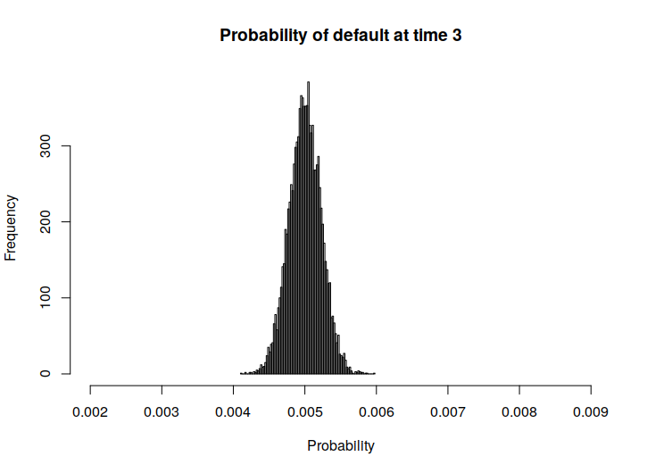
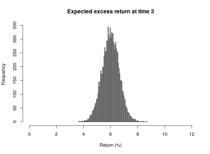
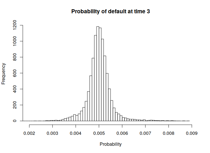
Below, in Figure 1 we also present some histograms of the actual returns and risks of ruin, in order to get a sense of the spread of these values.
 |
 |
 |
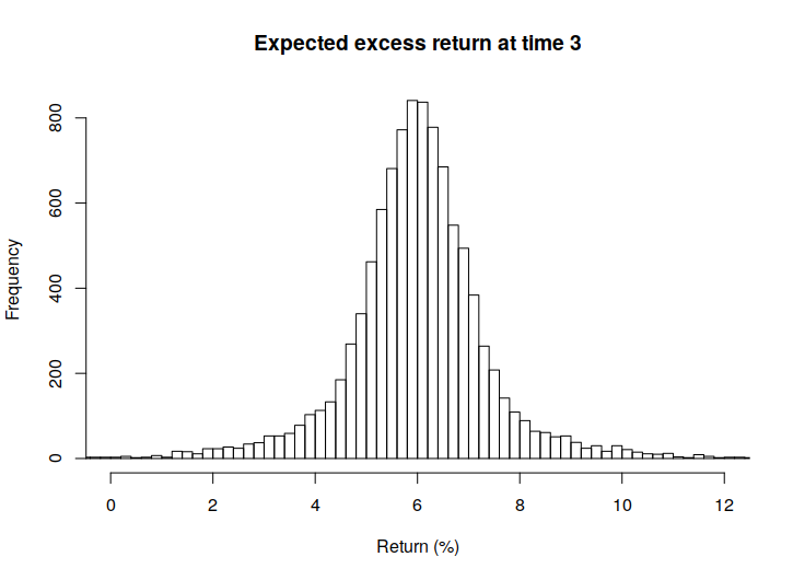 |
From these we can observe that the quantity representing the actual returns seems to be quite sensitive to model errors, if we recall the rather small size of the RMSE values.
| Model | Running time valuation (HH:MM) | Running time validation (HH:MM) |
|---|---|---|
| one single AR(1)-GARCH(1,1) | 00:06 | 00:10 |
| a sum of 10 AR(1)-GARCH(1,1) | 00:33 | 00:39 |
| Life model with 4 cohorts | 12:48 | 02:30 |
| Life model with 10 cohorts | 13:29 | 02:44 |
Table 4 displays the running times of each model. As far as is known, the main factor determining running time of Algoritm 1 is the repeated calculation of the basis functions inside the nested simulation (required to calculate the quantities in the inner for-loop). As these are quite many for models with high-dimensional state spaces, we see that running times increase accordingly. It should be noted that Algorithm 1 was not implemented to run as fast as possible for any specific model, other than the implementation of parallel programming. Speed could potentially be gained by adapting Algorithm 1 for specific models of interest.
Some conclusions can be drawn from the numerical results. Firstly, we can see that from a mean-squared-error point of view, the LSM model seems to work well in order to capture the dynamics of the multiperiod cost-of-capital valuation. It should be noted that the (N)RMSE of the value is lower than those of and across the board for all models and times. Since the expression for is heavily dependent of , we can suspect that estimation errors of and are positively correlated, and thus that gets lower mean squared errors as a result.
We can see that increasing model complexity for the AR(1)-GARCH(1,1) and life insurance models seems to have no significant effect on LSM performance. It should be noted that model complexity in both cases is increased by introducing independent stochastic factors; A sum of i.i.d. processes in the AR(1)-GARCH(1,1) case and the adding of (independent) cohorts in the life insurance case. Thus the de-facto model complexity might not have increased much, even though the state-space of the markov process is increased.
When we look at the ANDP and AROC quantities, we see that these seem to vary more than do the (N)RMSE:s. Especially AROC, which is defined via a quotient, seems to be sensitive to model error.
One important thing to note with regards to sensitivity of ANDP and AROC is the presence of errors introduced by the necessity of having to use Monte-Carlo simulations in order to calculate samples of . This can be seen in the AR(1)-GARCH(1,1) case: If we investigate what the value should be, we see that in this case it has a closed form (using positive homogeneity and translation invariance):
is deterministic due to law invariance. Since and are included in the basis functions for the AR(1)-GARCH(1,1) model, we would expect the fit in this case to be perfect. Since it is not, we conclude that errors still may appear even if optimal basis functions are among our selection of basis functions.
Finally, if we recall that the main purpose of these calculations is to calculate the quantity , a good approach for validation might be to re-balance the LSM estimates of and so that the LSM estimate of the value remains unchanged, but the LSM estimates are better fitted to and . This re-balancing would not be problematic in the economic model that this validation scheme is played out in. However, in this paper we were also interested in how the LSM model captures both the VaR term and the expected value term, so the quantities ANDP and AROC remain relevant to look at.
5 Conclusion
We have studied the performance of the LSM algorithm to numerically compute recursively defined objects such as given in definition 4, where the mappings are either -continuous or are given by (21). As a part of this study, Lipschitz-like results and conditions for -continuity were established for Value-at-Risk and the associated operator in Theorem 2 and Corollary 2. Important basic consistency results have been obtained showing the convergence of the LSM estimator both as the number of basis functions go to infinity in Lemmas 1 and 7 and when the size of the simulated data goes to infinity for a fixed number of basis functions in Theorems 1 and 3. Furthermore, these results are applicable to a large class of conditional monetary risk measures, utility functions and various actuarial multi-period valuations, the only requirement being -continuity or a property like that established in Theorem 2. We also apply and evaluate the LSM algorithm with respect to multi-period cost-of-capital valuation considered in [12] and [13], and in doing this also provide insight into practical considerations concerning implementation and validation of the LSM algorithm.
6 Proofs
Proof of Lemma 1.
Note that the quantities defined in (10) and (17) are independent of , hence all norms below are a.s. constants. Define . We will now show via backwards induction staring from time that . The induction base is trivial, since . Now assume that . Then
By the induction assumption and the continuity assumption, we know that the second summand goes to . We now need to show that . Now we simply note, by the definition of the projection operator and denseness of the approximating sets,
By our assumptions, both these terms go to zero as is afunction of the state , which lies in . ∎
Proof of Lemma 2.
We first note that if in probability, then in probability, since is independent of and -measurable, while is independent of . Hence it suffices to show that in probability. Now, recalling the definition of , we re-write (14) as
Furthermore recall the form of given by (13). We first note that since, by the law of large numbers, almost surely and thus in probability, it suffices to show that
in probability for each . We first note that, letting
The first summand goes to zero in probability by the law of large numbers. Thus, we investigate the second summand using Hölder’s inequality:
We see that, again by the law of large numbers, the first factor converges to in probability. Now we look at the second factor. By our independence assumption, and thus
which, by assumption, goes to in probability, hence the expression goes to zero in probability. This concludes the proof. ∎
Proof of Theorem 1.
We pove the statement by backwards induction, starting from time . As before, the induction base follows immediately from our assumptions. Now assume in probability, as . By -continuity we get that in probability. But then by Lemma 2 we immediately get that in probability. ∎
Proof of Lemma 3.
Note that
Here we have used Jensen’s inequality and the tower property of the conditional epectation at the second inequality and the following equality, respectively. From this -continuity immediately follows. ∎
Proof of Lemma 4.
By Lemma 9, to construct upper and lower bounds for a quantity given by we may find upper and lower bounds for and insert them into the expression for . Now Take and let . By monotnicity we get that
We now observe that
We use this to also observe that, by the subadditivity of the -operation,
Similarly, we have that
From this we get that
From which Lipschitz continuity with resepct to the constant immediately follows. ∎
Proof of Lemma 5.
By subadditivity we have that
Now we simply note that
This concludes the proof. ∎
Proof of Lemma 6.
Proof of Corollary 1.
Let . Now we simply note that, for any
By Markov’s inequality, we may bound the latter summand:
Now for the lower bound, we similarly note
where again we may bound the second summand using Markov’s inequality:
since we have assumed . This immediately yields that, almost surely,
This immediately yields our desired result. ∎
Lemma 9.
For any and with a.s.,
Proof of Lemma 9.
Let a.s. and let and . Note that almost surely, i.e. a.s. We now note that:
We look at the expectation in the first expression:
We now see that
This concludes the proof. ∎
Proof of Theorem 2.
Let . Note that
As for the -part of , including that in the expectation, we note that by Lemma 6 . We now note that, by subadditivity of ,
Hence
Here we have used the Markov’s inequality bound from Corollary 1.
We now similarly construct a lower bound for :
Again, for the -part, we note that by Lemma 6 . We now analyze the resulting expected value part, using subadditivity of :
Hence we get the lower bound
Here, again, we have used the Markov’s inequality bound from Corollary 1. Hence we have shown that
from which (24) immediately follows. ∎
Proof of Corollary 2.
Choose a sequence such that with and . We now use the following inequality, which follows from the monotonicity of in :
By -convergence and our choice of , the last term clearly goes to by our assumptions.
As for the first summand, we see that for any sequence , almost surely (by the continuity assumption of at ) and furthermore it is a decreasing sequence of nonnegative random variables in . Hence by Lebesgue’s monotone convergence theorem . This concludes the proof. ∎
Proof of Lemma 7.
By Lemma 2, is continuous with respect to limit objects with a.s. continuous -conditional distributions. Hence the proof is completely analogous to that of Lemma 1. ∎
Proof of Lemma 8.
Fix . we want to show that as . We first note that, for any with , we have an inequality similar to that in the proof of Corollary 2:
If we look at the first summand, we see that for any sequence , almost surely (by a.s. continuity) and furthermore it is a decreasing sequence of nonnegative random variables. Hence by Lebesgue’s monotone convergence theorem as a sequence of constants, since the expression is independent of .
We now apply Theorem 2 to the second term to see that
Note that is just a constant. We now note that, as in probability, then for any fixed , it is possible to choose a sequence such that . Hence, for any fixed , as . ∎
References
- [1] Philippe Artzner, Freddy Delbaen, Jean-Marc Eber, David Heath and Hyejin Ku (2007), Coherent multiperiod risk adjusted values and Bellman’s principle. Annals of Operations Research, 152, 5-22.
- [2] D. Barrera, S. Crépey, B. Diallo, G. Fort, E. Gobet and U. Stazhynski (2018), Stochastic approximation schemes for economic capital and risk margin computations. HAL <hal-01710394>
- [3] Mark Broadie, Yiping Du and Ciamac C. Moallemi (2015), Risk estimation via regression. Operations Research, 63 (5) 1077-1097.
- [4] Patrick Cheridito, Freddy Delbaen and Michael Kupper (2006), Dynamic monetary risk measures for bounded discrete-time processes. Electronic Journal of Probability, 11, 57-106.
- [5] Patrick Cheridito and Michael Kupper (2011), Composition of time-consistent dynamic monetary risk measures in discrete time. International Journal of Theoretical and Applied Finance, 14 (1), 137-162.
- [6] Patrick Cheridito and Michael Kupper (2009), Recursiveness of indifference prices and translation-invariant preferences. Mathematics and Financial Economics, 2 (3), 173-188.
- [7] Emanuelle Clément, Damien Lamberton, and Philip Protter(2002), An analysis of a least squares regression method for american option pricing. Finance and Stochastics, 6, 449–471.
- [8] European Commission (2015), Commission delegated regulation (EU) 2015/35 of 10 October 2014. Official Journal of the European Union.
- [9] Łukasz Delong, Jan Dhaene and Karim Barigou (2019), Fair valuation of insurance liability cash-flow streams in continuous time: Applications. ASTIN Bulletin, 49 (2), 299-333.
- [10] Kai Detlefsen and Giacomo Scandolo (2005), Conditional and dynamic convex risk measures. Finance and Stochastics, 9, 539-561.
- [11] Jan Dhaene, Ben Stassen, Karim Barigou, Daniël Linders and Ze Chen (2017) Fair valuation of insurance liabilities: Merging actuarial judgement and Market-Consistency. Insurance: Mathematics and Economics, 76, 14-27.
- [12] Hampus Engsner, Mathias Lindholm and Filip Lindskog (2017), Insurance valuation: A computable multi-period cost-of-capital approach. Insurance: Mathematics and Economics, 72, 250-264.
- [13] Hampus Engsner and Filip Lindskog (2020), Continuous-time limits of multi-period cost-of-capital margins. Statistics and Risk Modelling, forthcoming (DOI: https://doi.org/10.1515/strm-2019-0008)
- [14] Daniel Egloff (2005), Monte Carlo algorithms for optimal stopping and statistical learning, The Annals of Applied Probability, 15 (2), 1396-1432.
- [15] Hans Föllmer and Alexander Schied (2016), Stochastic finance: An introduction in discrete time, 4th edition, De Gruyter Graduate.
- [16] Francis A. Longstaff and Eduardo S. Schwartz (2001). Valuing American options by simulation: A simple least-squares approach. The Review of Financial Studies, 14 (1),113-147.
- [17] Christoph Möhr (2011), Market-consistent valuation of insurance liabilities by cost of capital. ASTIN Bulletin, 41, 315-341.
- [18] Antoon Pelsser and Ahmad Salahnejhad Ghalehjooghi (2020). Time-consistent and market-consistent actuarial valuation of the participating pension contract. Scandinavian Actuarial Journal, forthcoming (DOI: https://doi.org/10.1080/03461238.2020.1832911)
- [19] Antoon Pelsser and Ahmad Salahnejhad Ghalehjooghi (2016). Time-consistent actuarial valuations. Insurance: Mathematics and Economics, 66, 97-112.
- [20] Antoon Pelsser and Mitja Stadje (2014), Time-consistent and market-consistent evaluations. Mathematical Finance, 24 (1), 25-65.
- [21] Lars Stentoft (2004), Convergence of the least squares Monte Carlo approach to American option valuation. Management Science, 50 (9), 1193-1203.
- [22] John N. Tsitsiklis and Benjamin Van Roy (2001). Regression methods for pricing complex American-style options. IEEE Transactions On Neural Networks, 12 (4), 694-703.
- [23] Daniel Z. Zanger (2009), Convergence of a least-squares Monte Carlo algorithm for bounded approximating sets. Applied Mathematical Finance, 16 (2), 123-150.
- [24] Daniel Z. Zanger (2013), Quantitative error estimates for a least-squares Monte Carlo algorithm for American option pricing. Finance and Stochastics, 17, 503-534.
- [25] Daniel Z. Zanger (2018), Convergence of a least-squares Monte Carlo algorithm for American option pricing with dependent sample data. Mathematical Finance, 28 (1), 447-479.