11email: Marek.Abramowicz@physics.gu.se 22institutetext: N. Copernicus Astronomical Center, Polish Academy of Sciences, Bartycka 18, PL-00-716 Warszawa, Poland
22email: as@camk.edu.pl, 22email: agata@camk.edu.pl 33institutetext: Warsaw University Observatory, Al. Ujazdowskie 4, PL-00-478 Warszawa, Poland
33email: mj@astrouw.edu.pl 44institutetext: 2-2-2 Shikanodai-Nishi, Ikoma-shi, Nara 630-0114, Japan
44email: kato.shoji@gmail.com, 44email: kato@kusastro.kyoto-u.ac.jp 55institutetext: Institut d’Astrophysique de Paris, UMR 7095 CNRS, UPMC Univ Paris 06, 98bis Bd Arago, 75014 Paris, France
55email: lasota@iap.fr 66institutetext: Jagiellonian University Observatory, ul. Orla 171, PL-30-244 Kraków, Poland 77institutetext: Institute of Physics, Faculty of Philosophy and Science, Silesian University in Opava, Bezručovo nám. 13, 746-01 Opava, Czech Republic
Leaving the ISCO: the inner edge of a black-hole accretion disk
at various luminosities
The “radiation inner edge” of an accretion disk is defined as the inner boundary of the region from which most of the luminosity emerges. Similarly, the “reflection edge” is the smallest radius capable of producing a significant X-ray reflection of the fluorescent iron line. For black hole accretion disks with very sub-Eddington luminosities these and all other “inner edges” locate at ISCO. Thus, in this case, one may rightly consider ISCO as the unique inner edge of the black hole accretion disk. However, even for moderate luminosities, there is no such unique inner edge as differently defined edges locate at different places. Several of them are significantly closer to the black hole than ISCO. The differences grow with the increasing luminosity. For nearly Eddington luminosities, they are so huge that the notion of the inner edge losses all practical significance.
Key Words.:
black holes – accretion disks – inner edge1 Introduction
Accretion flows on to black holes must change character before matter crosses the event horizon. Two reasons account for this fundamental property of such flows. First, matter must cross the black-hole surface at the speed of light as measured by a local inertial observer (see e.g. Gourgoulhon & Jaramillo 2006), so that if the flow is sub-sonic far away from the black-hole (in practice it is always the case) it will have to cross the sound barrier (well) before reaching the horizon. This is the property of all realistic flows independent of their angular momentum. The sonic surface in question can be considered as the inner edge of the accretion flow.
The second reason is related to angular momentum. Far from the hole many (most probably most) rotating accretion flows adapt the Keplerian angular momentum profile. Because of the existence of the Inner-Most Stable Circular Orbit (ISCO) such flow must stop to be Keplerian there. At high accretion rates when pressure gradients become important the flow may extend below the ISCO but the presence of the Inner-Most Bound Circular Orbit (IBCO) defines another limit for a circular flow (the absolute limit being given by the Circular Photon Orbit; the CPO). These critical circular orbits provide another possible definition of the inner edge of the flow, in this case of an accretion disk.
The question is: what is the relation between the accretion flow edges? In the case of geometrically thin disks the sonic and Keplerian edges coincide and one can define the ISCO as the inner edge of such disks. Paczyński (2000) showed rigorously that, independent of viscosity mechanism, presence of magnetic fields etc. the ISCO is the universal inner disk’s edge for not too-high viscosities. The case of thin disks is therefore settled111In a recent paper Penna et al. (2010) studied the effects of magnetic fields on thin accretion disk (the disk thickness , which corresponds to ). They found that to within a few percent the magnetized disks are consistent with the Novikov & Thorne (1973) model, in which the inner edge coincides with the ISCO..
However, this is not the case of non-thin accretion disks, i.e. the case of medium and high luminosities. The problem of defining the inner edge of an accretion disk is not just a formal exercise. Afshordi & Paczyński (2003) explored several reasons which made discussing the location of inner edge of the black hole accretion disks an interesting and important issue. One of them was,
Theory of accretion disks is several decades old. With time ever more sophisticated and more diverse models of accretion onto black holes have been introduced. However, when it comes to modeling disk spectra, conventional steady state, geometrically thin-disk models are still used, adopting the classical “no torque” inner boundary condition at the marginally stable orbit.
The best illustration of this fact is the case of the state-of-art works on measuring the black hole spin in the microquasar GRS 1915+105 by fitting its observed “thermal state” spectra to these calculated (e.g. Shafee et al. 2008; Middleton et al. 2009). These works use general relativistic version of the classical Shakura-Sunyaev thin accretion disk model worked out by Novikov & Thorne (1973). The Novikov-Thorne model assumes that the inner edge of the the disk is also the innermost boundary of the radiating region.
Because the black hole mass of GRS 1915+105 is known and therefore fixed (), the surface area of the radiating region, calculated in the model, depends only on the black hole unknown spin, ( with being the total angular momentum of the black hole). In the thermal state, the disk spectrum is close to that of a sum of black body contributions from different radial locations. Its shape is determined by the radial distribution of temperature, which in the Novikov-Thorne model depends on the spin, . The total radiation power is determined by the “averaged” temperature and the surface area of the radiating region, . By calculating the spectral shape and power for different in the Novikov-Thorne model, one may find the best-fit estimates for the spin-dependent temperature and area. This is just the main idea of the spin estimate; details of the fitting are far more complex (see Shafee et al. 2008; Davis et al. 2005; Straub et al. 2010) and include, for example, a heuristic way of treating a contribution of scattering in accretion disks atmosphere (i.e. the “hardening factor”).
Results obtained this way by Shafee et al. (2008) for GRS 1915+105 showed that for the whole luminosity range . However, for , the spin estimated by Shafee et al. (2008) was much lower, . The inconsistent spin estimates at different luminosities indicate that some assumptions adopted by the Novikov-Thorne model are wrong at high luminosities.
This is not a surprise, because there are several physical effects known to be important at high luminosities, but ignored in the classical Shakura-Sunyaev and Novikov-Thorne thin accretion disk models. These effects are properly included in the slim222The names thin and slim refer to the dimensionless vertical geometrical thickness, . For thin disks it must be , while for slim disks a weaker condition holds. accretion disks models, introduced by Abramowicz et al. (1988). Advection is perhaps the best known of these “slim disk effects”, but in the present context equally important is a significant stress due to the radial pressure gradient (for thin disks ). The stress firmly holds matter well inside ISCO and as a result of this, at high luminosities the edge of the plunge-in region may be considerably closer to the black hole than ISCO333Matter may be hold well inside ISCO also by magnetic stresses, as pointed out by many authors; see e.g. a semi-analytic model by Narayan et al. (2003), or MHD numerical simulations by Noble, Krolik & Hawley (2010), and references quoted in these papers..
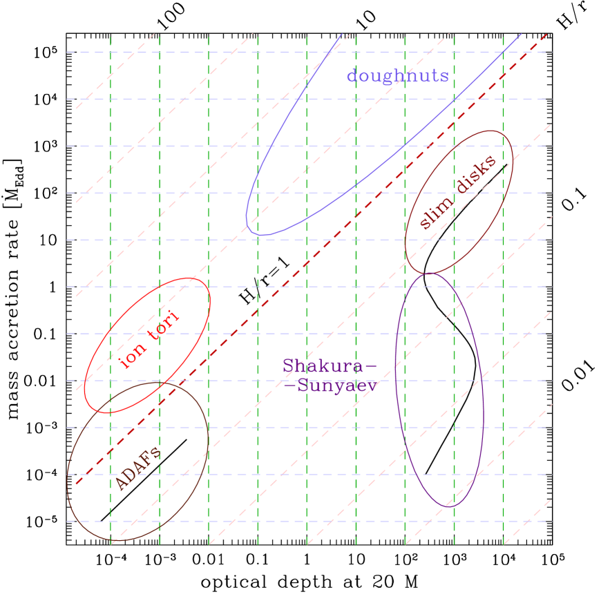
Slim disks are assumed to be stationary and axially symmetric. They are described by vertically integrated Navier-Stokes hydrodynamical equations; no magnetic fields are considered. The effective viscosity, believed to be generated by the MHD turbulence (Balbus & Hawley 1991) is described by the “” Shakura-Sunyaev ansatz. Figure 1 shows the slim disk location with respect to other analytic and semi-analytic disk models, in the parameter space described by the vertical optical depth , dimensionless vertical thickness and dimensionless accretion rate , where is the critical accretion rate approximately corresponding to the Eddington luminosity (erg/s) in case of a disk around a non-rotating black hole444Two warnings about notation. (i) Many authors use a different definition, . (ii) We often use the convention in which ..
In this paper, we discuss properties of the inner edge of slim accretion disks around rotating black holes, using models similar to those calculated recently by S\kadowski (2009)555At http://users.camk.edu.pl/as/slimdisks a very detailed data base for these solutions is given. It covers the whole parameter space relevant for microquasars and AGN.. For convenience, we shortly remind the slim disk basic equations in the Appendix A. In the following Section 2, we list six possible definitions of the inner edge. These definitions reflect different (but partially overlapping) physical meanings and different practical astrophysical applications. In the following six Sections 3-8 we calculate the slim disk locations of these six inner edges, and discuss their astrophysical relevance. Some of the results presented here have been anticipated previously by us and other authors in a different context of the Polish doughnuts (i.e. thick accretion disks; see e.g. a short review by Paczyński 1998); see also Paczyński (2000) and Afshordi & Paczyński (2003).
2 Definitions of the inner edge
Krolik & Hawley (2002) proposed several “empirical” definitions of the inner edge, each serving a different practical purpose (see also the follow-up by Beckwith et al. 2002). We add to these a few more definitions. The list of the inner edges considered in this paper consists of666Krolik & Hawley defined [4], [5], [6] above and in addition [7], the turbulence edge, where flux-freezing becomes more important than turbulence in determining the magnetic field structure. Magnetic fields are not considered for slim accretion disks, and we will not discuss [7].,
[1] The potential spout edge , where the effective potential forms a self-crossing Roche lobe, and accretion is governed by the Roche lobe overflow.
[2] The sonic edge , where the transition from subsonic to transonic accretion occurs. Hydrodynamical disturbances do not propagate upstream a supersonic flow, and therefore the subsonic part of the flow is “causally” disconnected from the supersonic part.
[3] The variability edge , the smallest radius where orbital motion of coherent spots may produce quasi periodic variability.
[4] The stress edge , the outermost radius where the Reynolds stress is small, and plunging matter has no dynamical contact with the outer accretion flow;
[5] The radiation edge , the innermost place from which significant luminosity emerges.
[6] The reflection edge , the smallest radius capable of producing significant fluorescent iron line.
In the next six Sections we discuss the six edges one by one.
3 The potential spout edge
The idea of the “relativistic Roche lobe overflow” governing accretion close to the black hole was first explained by Paczyński (see Kozłowski et al. 1978). Later, it was explored in detail by many authors analytically (e.g. Abramowicz 1981, 1985) and by large-scale hydrodynamical simulations (e.g. Igumenshchev & Beloborodov 1997). It became a standard concept in the black hole accretion theory. Figure 2 schematically illustrates the Roche lobe overflow mechanism. The left-most panel presents demonstrative profile of disk angular momentum which reaches the Keplerian value at the radius corresponding to the self-crossing of the equipotential surfaces presented in the middle panel. To flow through this “cusp” matter must have potential energy higher than the value of the potential at this point - such “potential barrier” is crossed only when the matter overflows its Roche lobe. Precise profiles of the potential barriers and the angular momentum, calculated with the slim disk model, are presented in Figs. 3 and 4 , respectively.
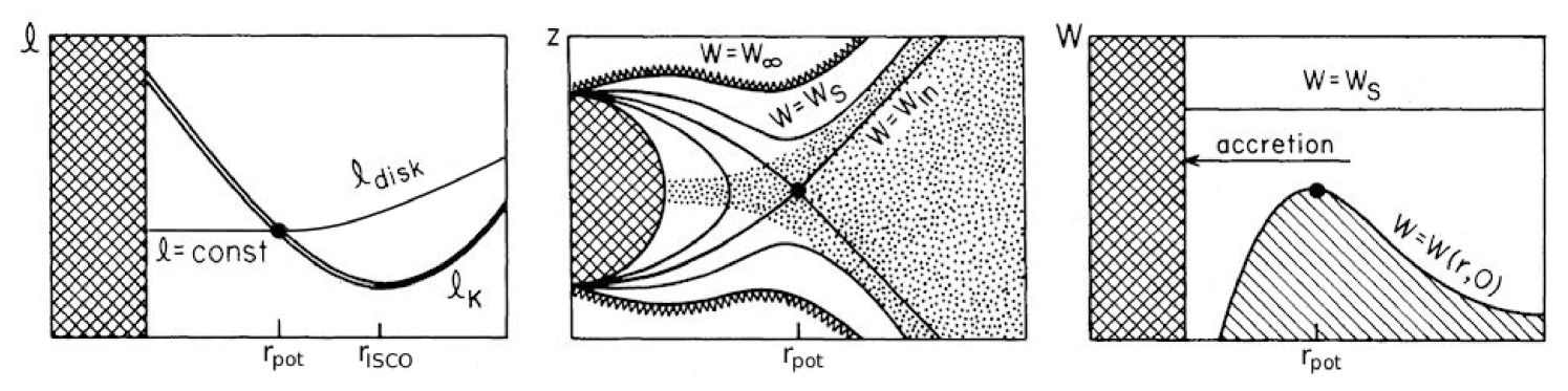

The potential difference between the horizon and the spout is infinite, and therefore no stress may prevent the matter located there from plunging into the black hole. For radii greater that , the potential barrier at holds the matter in. Note, that because the dynamical equilibrium is given (approximately) by , with being the density, one may also say that it is the pressure gradient (the pressure stress) that holds the matter inside .
The specific angular momentum in the Novikov-Thorne model is assumed to be Keplerian. Slim disk models do not a priori assume an angular momentum distribution, but self-consistently calculate it from the relevant equations of hydrodynamics (15)-(22). These calculations reveal that the type of angular momentum distribution depends on whether accretion rate and viscosity locate the flow in the disk-like, or the Bondi-like type.
In the Bondi-type accretion flows the angular momentum is everywhere sub-Keplerian, . These flows are typical for high viscosities and high accretion rates, as in the case of and shown in Figure 4. This is the only Bondi-like flow in this Figure.

In the disk-like accretion flows, the angular momentum of the matter in the disk is sub-Keplerian everywhere, except the strong-gravity region where the flow is super-Keplerian, . The radius corresponds to the ring of the maximal pressure in the accretion disk. This is also the minimum of the effective potential. The radius marks a saddle point for pressure and effective potential; this is also the location of the “potential spout inner edge”, .
Note that in the classic solutions for spherically accretion flows found by Bondi (1952) the viscosity is unimportant and the sonic point is saddle, while in the “Bondi-like” flows discussed here, angular momentum transport by viscosity is essentially important and the sonic point is usually nodal. Therefore, one should keep in mind that the difference between these types of accretion flows is also due to the relative importance of pressure and viscosity. For this reason a different terminology is often used. Instead of “disk-like” one uses the term “pressure-driven” and instead of “Bondi-like” one uses “viscosity-driven” (see e.g. Matsumoto et al. 1984; Kato et al. 2008).
From the above discussion it is clear that the location of this particular inner edge is formally given as the smaller of the two roots, , of the equation
| (1) |
The larger root corresponds to . Obviously, equation (1) has always a solution for the disk-like flows, and never for the Bondi-like flows. Figure 5 shows a division of the parameter space into regions occupied by Bondi-like and disk-like flows.

The location of the potential spout inner edge is shown in Figure 6 for . Note that for small accretion rates, , location of the potential spout inner edge coincides with ISCO. At , the location of the potential spout jumps to a new position, which is close to the radius of the innermost bound circular orbit, . This behavior is now well-known. It was noticed first by Kozłowski et al. (1978) for Polish doughnuts, and by Abramowicz et al. (1988) for slim disks.

We conclude the Section on the potential spout inner edge by giving an approximate formula for its location,
| (2) | |||||
The formula (2) is valid for .
4 The sonic edge
By a series of algebraic manipulations one reduces the slim disk equations (15)-(22) to a set of two ordinary differential equations for two dependent variables, e.g. the Mach number and the angular momentum ,
| (3) |

For a non-singular physical solution the nominators and must vanish at the same radius as the denominator . The denominator vanishes at the sonic edge (or sonic radius) where the Mach number is close to unity, i.e.
| (4) |
For low mass accretion rates, smaller than about in case of , the sonic edge locates close to ISCO, independently on the viscosity , as Figure 7 shows. At about a qualitative change occurs, resembling a “phase transition” from the Shakura-Sunyaev behavior, to a very different slim-disk behavior.
For higher accretion rates the location of the sonic point significantly departs from ISCO. For low values of the sonic point moves closer to the horizon down to for . For the sonic point moves outward with increasing accretion rate reaching values as high as for and . This effect was first noticed for small accretion rates by Muchotrzeb-Czerny (1986) and later investigated in a wide range of accretion rates by Abramowicz et al. (1988), who explained it in terms of the disk-Bondi dichotomy. The dependence of the sonic point location on the accretion rate in the near-Eddington regime is more complicated and is related to the fact that in this range of accretion rates the transition from the radiatively efficient disk to the slim disk occurs near the sonic radius.
The topology of the sonic point is important, because physically acceptable solutions must be of the saddle or nodal type; the spiral type is forbidden. The topology may be classified by the eigenvalues of the Jacobi matrix,
| (5) |
Because , only two eigenvalues are non-zero, and the quadratic characteristic equation that determines them takes the form,
| (6) |
The nodal type is given by and the saddle type by , as marked in Figure 7 with the dotted and the solid lines, respectively. For the lowest values of only the saddle type solutions exist. For moderate values of () the topological type of the sonic point changes at least once with increasing accretion rate. For the highest solutions have only nodal type critical points.
The extra regularity conditions at the sonic point are satisfied only for one particular value of the angular momentum at the horizon which is the eigenvalue of the problem. is not known a priori, and should be found. Figure 8 shows how does depend on the accretion rate and the viscosity parameter.

5 The variability edge
Axially symmetric and stationary states of slim accretion disks represent, obviously, only a certain theoretical idealization. Real disks are non-axial and non-steady. In particular, one expects transient coherent features at accretion disk surfaces — clumps, flares, and vortices. Orbital motion of these features could quasi-periodically modulate the observed flux of radiation, mostly through the Doppler effect and the relativistic beaming. Let be the “averaged” variability period, and a change of the period during one period due to radial motion of a spot.

The variability quality factor may be estimated by,
| (7) |
where and and are contravariant components of the four velocity. The period relates to the orbital angular velocity by . Using the relations (see Appendix A for the explanation of the notation used),
| (8) |
with being the radial velocity as measured by an observer corotating with the fluid, one obtains:
| (9) |
where,
| (10) |
with . From (16) and (19) it is clear than outside the black hole horizon. Note that in Newtonian limit it is and one has . In this limit , are the radial and azimuthal component of velocity, and the formula (9) takes its obvious Newtonian form.

Behavior of the quality factor is shown in Figure 10. Profiles for four accretion rates are drawn. As Fig. 9 shows the lower accretion rate the smaller radial velocity component and therefore the quality factor in general increases with decreasing accretion rate. For the lowest values of a rapid drop is visible at ISCO corresponding to the change in the nature of the flow (gas enters the free-fall region below ISCO). For higher accretion rates such behaviour is suppressed as the trajectories become wide open spirals well outside ISCO.
Note that our definition (7) of the quality factor , essentially agrees with a practical definition of the variability quality factor defined by observers with the help of the observationally constructed Fourier variability power spectra, . Here is the observed variability power (i.e. the square of the observed amplitude) at a particular observed variability frequency . Any observed quasi periodic variability with the frequency shows in the power spectrum as a local peak in , centered at a certain frequency . The half-width of the peak defines the variability quality factor by .
Quasi periodic variability with kHz frequencies, called kHz QPO, is observed from several low-mass neutron star and black hole binaries. In a pioneering and important research, Barret et al. (2005) carefully measured the quality factor for a particular source in this class (4U 1608-52) and found that , i.e. that the kHz are very coherent. They argued that cannot be due to kinematic effects in orbital motion of hot spots, clumps or other similar features located at the accretion disk surface, because these features are too quickly sheared out by the differential rotation of the disk (see also Bath et al. 1974; Pringle 1981). They also argued that although coherent vortices may survive much longer times at the disk surface (e.g. Abramowicz et al. 1995), if they participate in the inward radial motion, the observed variability cannot be high. Our results shown in Figure 10 illustrate and strengthen this point. We also agree with the conclusion reached by Barret et al. (2005) that the observational evidence against orbiting clumps as a possible explanation of the phenomenon of kHz QPO, seems to point out that this phenomenon is most probably due to the accretion disk global oscillations777Barret et al. (2005) found also how varies in time for each of the two individual oscillations in the “twin-peak QPO”. This gives strong observational constraints for possible oscillatory models of the twin peak kHZ QPO; see also Boutelier et al. (2010).. For excellent reviews of the QPO oscillatory models see Wagoner (1999) and Kato (2001).
Although clumps, hot-spots, vortices or magnetic flares cannot explain the coherent kHz QPOs with , they certainly are important in explaining the continuous, featureless Fourier variability power spectra (see e.g. Abramowicz et al. 1991; Schnittman 2005; Pecháček, Karas & Czerny 2008, and references quoted there). Our results shown in Figure 10 indicate that: (i) at low accretion rates, a sharp high-frequency cut-off in may be expected at about the ISCO frequency, (ii) at high accretion rates there should be no cut-off in at any frequency, (iii) the logarithmic slope should depend on .
A more quantitative description of (i)-(iii) will be given in a future publication (Straub 2010).
6 The stress edge
The Shakura-Sunyaev model assumes that there is no torque at the inner edge of the disk, which in this model coincides with ISCO. Slim disk model assumes that there is no torque at the horizon of the black hole. It makes no assumption on the torque at the disk inner edge, but calculations prove that the torque is small there.
The zero-torque at the horizon is consistent with the small torque at the inner edge of slim disks, as Figure 11 shows.


The Figure presents the relative importance of the torque by comparing it with the “advective” flux of angular momentum (c.f. equation 23). For the viscosity parameter smaller than about , the ratio both at and is smaller than even for highly super-Eddington accretion rates, and for small accretion rates the ratio is vanishingly small, . For high viscosity, , the ratio is very small for small accretion rates, and still smaller than about even for super-Eddington accretion rates (calculated at the sonic radius as the disk enters the Bondi-like regime for such high accretion rates).

To define the stress inner edge one has to specify the characteristic value of the torque parameter . Profiles of for a few values of and are shown in Fig. 12. The stress edge for is located at ISCO for low accretion rates. When accretion rate exceeds it departs from ISCO and moves closer to BH approaching its horizon with increasing . Behaviour of profiles for higher () values of is different - they move away from the BH as the angular momentum profiles become flatter with increasing accretion rates (compare Fig. 4).
In the case of disk-like accretion with a very low viscosity , it is with high accuracy,
| (11) |
In this case the “inner edge” inherits both the sonic edge and the potential spout edge properties; suggesting a small torque. It looks, as this is indeed the case. By pushing the MHD numerical simulations to their limits, Shafee et al. (2008) and recently Penna et al. (2010) calculated a thin, , disk-like accretion flow, and showed that for it the inner edge torque was small.
7 The radiation edge
As discussed in the previous section, the torque at is small, but non-zero and therefore there is orbital energy dissipation also at radii smaller than ISCO. Thus, some radiation from this region takes place and the inner edge is not expected to coincide with the radiation edge, . In Fig. 13 we present profiles of defined as radii limiting area emitting given fraction of disk total luminosity. For low accretion rates () disk emission terminates close to ISCO as the classical models of accretion disks predict. Locations of the presented are determined by the regular Novikov & Thorne flux radial profile. For higher accretion rates disk becomes advective and the maximum of the emission moves significantly inward. As a consequence of the increasing rate of advection (and resulting inward shift of ) the efficiency of accretion drops down.
We want to stress here that the location of the radiation edge is not determined by the location of the stress edge (as some authors seem to believe), but by the fact that significant advection flux brings energy into the region well below ISCO.
Let be the outer radius of the disk. The total luminosity of the disk could be estimated from
| (12) |
It is , , and from this one derives
| (13) |
where is the ratio of the viscous torque to the advective flux of angular momentum (see Figures 11 and 12).
Because , the efficiency of accretion depends mainly on the specific energy at the inner edge, . The further away is the inner edge from ISCO (and closer to the black hole), the smaller is the efficiency.

8 The reflection edge
The iron Kα fluorescent line is one of the characteristic features observed in many sources with black hole accretion disks (Miller 2006; Remillard & McClintock 2006). The intensity and the shape of this line depends strongly on the physical conditions close to the inner edge. This was discussed by many authors, including Reynolds & Fabian (2008) who gave three conditions for line formation: (i) the flow has to be Thomson-thick in the vertical direction; (ii) disk has to be irradiated by external source of X-rays (hard X-ray irradiation plays crucial role in the process of fluorescence and changes the ionization degree of matter); (iii) the ionization state should be sufficiently low (iron cannot be fully ionized).
We point out here, that this first condition is sufficient for the formation of the reflection continuum, but formation of the fluorescent iron line requires an even stronger condition i.e. that the effective optical depth of the flow should be higher than unity:
| (14) |
This is because, the fluorescence requires efficient absorption of high energy photons by iron ions. In Fig. 14 we present profiles of the effective optical depth in different regimes of accretion rates for and . Three characteristic types of their behaviour are shown: sharp drop, maximum and monotonic at the top, middle and bottom panels, respecively. Behaviour for different values of and is qualitatively similar (but not quantitatively as in general increases with decreasing ). Top panel, corresponding to the lowest accretion rates, shows a sharp drop in near ISCO. The same behavior was noticed previously e.g. by Reynolds & Fabian (2008). The drop could clearly define the inner reflection edge limiting the radii where formation of the fluorescent iron line is prominent. The middle panel, corresponding to moderate accretion rates, shows a maximum in near ISCO. The non-monotonic behaviour is caused by the fact that regions of moderate radii outside ISCO become radiation pressure and scattering dominated. Note, that the top of the maximum of stays near ISCO in a range of accretion rates, but for accretion rates greater than it moves closer to the black hole with increasing as the disk emission profile changes due to advection. The bottommost panel corresponds to super-Eddington accretion rates. The profiles are monotonic in and define no characteristic inner reflection edge. Close to the black hole such flows are effectively optically thin reaching on about few tens of gravitational radii.
When effective optical depth of the flow becomes less then unity, our approximation of radiative transfer by diffusion with grey opacities (Eq. 22) becomes not valid. In such case full radiative transfer through accretion disks atmospheres should be solved (e.g. Davis et al. 2005; Różańska & Madej 2008). Still, our results allow us to estimate roughly how far from the black hole the iron line formation is most prominent, assuming that disk is uniformly illuminated by an exterior X-ray source. For accretion rates smaller than , the reflection edge is located very close to ISCO and we may identify shape of the iron line with gravitational and dynamical effects connected to ISCO. In case of higher but sub-Eddington accretion rates, the maximum of the effective optical depth is located inside ISCO what may possibly allow us to study extreme gravitational effects on the iron line profile. However, the assumption that the line is formed at ISCO is no longer satisfied. The super-Eddington flows have smooth and monotonic profiles of the effective optical depth. Therefore, the reflection edge cannot be uniquely defined and no relation between shape of the fluorescent lines and ISCO exists. Finally, one should keep in mind that such lines can be successfully modeled by clumpy absorbing material and may have nothing to do with relativistic effects (see e.g. Miller et al. 2009, and references therein). The role of the ISCO in determining the shape of the Fe lines was also questioned in the past (based on different reasoning) by Reynolds & Begelman (1997) whose arguments were then refuted by Young et al. (1998).


9 Conclusions
We addressed the inner edge issue by discussing behavior of six differently defined “inner edges” of slim accretion disks around the Kerr black hole. We found that the slim disk inner edges behave very differently than the corresponding Shakura-Sunyaev and Novikov-Thorne ones. The differences are qualitative. Even for moderate luminosities, , there is no unique inner edge. Differently defined edges locate at different places. For nearly Eddington luminosities, the differences are huge and the notion of the inner edge losses all practical significance.
We summarize the properties and locations of the six inner edges in Table 1. It refers to , but the qualitative behavior is similar for .
| for moves inward with increasing down to ; for and sufficiently high disk enters the Bondi regime — undefined | departs from ISCO; for ; for | undefined | moves inward with increasing down to BH horizon. | moves inward with increasing down to BH horizon. | for for undefined | ||
We conclude, by showing in Figure 15 differences between the Shakura-Sunyaev and slim-disk (in the disk-like case) treatment of the inner disk physics. The innermost part of a Shakura-Sunyaev disk is shown in the left column in Figure 15, and the innermost part of a slim disk is shown in the right column. The upper panel shows angular momentum in the disk (the solid line) in reference to the Keplerian distribution (the dashed line). ISCO, indicated by the dash-dotted line is at the radius where the Keplerian angular momentum has its minimum. The potential spout (a square) and the center (a triangle) are defined as crossings of the angular momentum in the disk line with the Keplerian line. For slim disks they are at two different radii, on both sides of the ISCO. For Shakura-Sunyaev disks they merge into one singular location at ISCO. The lower panel shows the cross section of the disk. The slim disk has everywhere a finite thickness while the Shakura-Sunyaen disk is singular at ISCO (it has a zero thickness there). The sonic radius (a cross) is where the accretion component of the velocity equals the local sound speed. In slim disks, the sonic point corresponds to a critical point of the set of differential equations, that through the regularity conditions defines the global eigensolution of the problem. The Shakura-Sunyaev disk is described by local algebraic equations and this global eigenvalue aspect is missing, thus location of a sonic point is of no relevance.

Acknowledgements.
This work was supported by Polish Ministry of Science grants N203 0093/1466, N203 304035, N203 380336, N203 00832/0709. AS acknowledges support from the Department of Astronomy at Kyoto University. MAA acknowledges a professorship at Université Pierre et Marie Curie that supported his visit to Institut d’Astrophysique in Paris during which a part of research reported here was done. MAA also acknowledges the Czech government grant MSM 4781305903. JPL acknowledges support from the French Space Agency CNES.References
- Abramowicz (1981) Abramowicz M.A., 1981, Nature, 294, 235
- Abramowicz (1985) Abramowicz M.A., 1985, PASJ, 37, 727
- Abramowicz et al. (1991) Abramowicz M.A., Bao G., Lanza A., & Zhang X.-H., 1991, A&A, 245, 454
- Abramowicz et al. (1996) Abramowicz M.A., Chen X.-M., Granath M. & Lasota, J.-P., 1996, ApJ, 471, 762
- Abramowicz et al. (1988) Abramowicz M.A., Czerny B. & Lasota J.-P., 1988, ApJ, 332, 646
- Abramowicz et al. (1978) Abramowicz M.A., Jaroszyński M., & Sikora M., 1978, A&A, 63, 221
- Abramowicz et al. (1995) Abramowicz M.A., Lanza A., Spiegel E.A., Szuszkiewicz E., 1992, Nature, 356, 41
- Abramowicz & Zurek (1981) Abramowicz M.A. & Zurek W.H., 1981, ApJ, 246, 314
- Afshordi & Paczyński (2003) Afshordi N., & Paczyński B., 2003, ApJ, 592, 354
- Agol & Krolik (2000) Agol E. & Krolik J.H., 2000, ApJ, 528, 161
- Balbus & Hawley (1991) Balbus S.A. & Hawley J.F., 1991, ApJ376, 214
- Barret et al. (2005) Barret D., Kluźniak W., Olive J.F., Paltani S., Skinner G.K., 2005, MNRAS, 357, 1288
- Bath et al. (1974) Bath G.T., Evans W.D., Papaloizou J., 1974 MNRAS167, 7p
- Beckwith et al. (2002) Beckwith K., Hawley J.F. & Krolik J.H. 2008, MNRAS, 390, 21
- Blandford & Znajek (1977) Blandford, R.D.; Znajek, R.L., 1977, MNRAS179, 433
- Bondi (1952) Bondi H., 1952, MNRAS112, 195
- Boutelier et al. (2010) Boutelier M., Barret D., Lin Y., Török G., 2010, MNRAS, 401, 1290
- Davis et al. (2005) Davis S.W., Blaes O.M., Hubeny I., Turner N.J., 2005, ApJ621, 372
- Gourgoulhon & Jaramillo (2006) Gourgoulhon, E., & Jaramillo, J. L. 2006, Phys. Rep, 423, 159
- Hawley et al. (2001) Hawley, J. F., Balbus, S. A., & Stone, J. M., 2001, ApJ, 554, 49
- Esin et al. (1997) Esin, A.A., McClintock, J.E., & Narayan, R., 1997, ApJ, 489, 865
- Frank et al. (2002) Frank J., King A. & Raine D., 2002, Accretion Power in Astrophysics, Cambridge University Press (3rd edition)
- Gammie (1999) Gammie, C.F. 1999, ApJ, 522, L57
- Gammie & Popham (1998) Gammie, C. F., & Popham, R. 1998, ApJ, 498, 313
- Igumenshchev & Beloborodov (1997) Igumenshchev I.V., Beloborodov A.M., 1997 MNRAS284, 767
- Jaroszyński et al. (1980) Jaroszyński M., Abramowicz M.A. & Paczyński B., 1980, Acta Astr., 30, 1
- Kato et al. (2008) Kato S., Fukue J. & Mineshige S. 2008, Black-Hole Accretion Disks — Towards a New Paradigm, Kyoto University Press (2nd edition)
- Kato (2001) Kato S., 2001, PASJ, 53, 1
- Krolik (2002) Krolik, J.H., 1999 ApJ, 515, L73
- Krolik & Hawley (2002) Krolik J.H. & Hawley J.F. 2002, ApJ, 573, 754
- Komissarov (2006) Komissarov S.S., 2006 MNRAS368, 993
- Komissarov (2008) Komissarov, S.S., 2008, preprint arXiv:0804.1912
- Kozłowski et al. (1978) Kozłowski M. & Abramowicz M.A. & Jaroszyński M. 1978, A&A, ,
- Lasota (1994) Lasota, J. P. 1994, in NATO ASIC Proc. 417: Theory of Accretion Disks - 2, ed. W. J. Duschl, J. Frank, F. Meyer, E. Meyer-Hofmeister, & W. M. Tscharnuter, 341–+
- Matsumoto et al. (1984) Matsumoto, R., Kato, S., Fukue, J., & Okazaki, A. T. 1984, PASJ, 36, 71
- Middleton et al. (2009) Middleton M., Done C., Ward M., Gierliśki M., Schurch N. 2009, MNRAS394, 250
- Miller (2006) Miller, J. M. 2006, Astronomische Nachrichten, 327, 997
- Miller et al. (2009) Miller, L., Turner, T. J., & Reeves, J. N. 2009, MNRAS, 399, L69
- Muchotrzeb & Paczyński (1982) Muchotrzeb, B. & Paczyński, B., 1982, Acta Astr., 32, 1
- Muchotrzeb (1983) Muchotrzeb, B., 1983, Acta Astr., 33, 79
- Muchotrzeb-Czerny (1986) Muchotrzeb-Czerny, B., 1986, Acta Astr., 36, 1
- Narayan & Yi (1988) Narayan R., Yi I., 1988, ApJ, 444, 231
- Narayan et al. (2003) Narayan, R.; Igumenshchev, I.V. & Abramowicz, M.A., 2003, PASJ, 55. L69
- Noble, Krolik & Hawley (2010) Noble S.C., Krolik J.H., Hawley J.F., 2010 ApJin press, arXiv:1001.4809v1 [astro-ph.HE] 26 Jan 2010
- Novikov & Thorne (1973) Novikov, I. D., & Thorne, K. S. 1973, Black Holes (Les Astres Occlus), 343
- Paczyński (2000) Paczyński, B. 2000, preprint, arXiv:astro-ph/0004129
- Paczyński (1998) Paczyński, B. 1998, preprint., astro-ph-0004129
- Paczyński & Bisnovatyi-Kogan (1981) Paczyński, B. & Bisnovatyi-Kogan, G., 1981, Acta Astr., 31, 283
- Paczyński & Wiita (1980) Paczyński, B. & Wiita, P.J., 1980, å, 88, 23
- Pecháček, Karas & Czerny (2008) Pecháček T., Karas V., Czerny B., 2008 A&A, 487, 815
- Penna et al. (2010) Penna, R. F., McKinney, J. C., Narayan, R., Tchekhovskoy, A., Shafee, R., & McClintock, J. E. 2010, arXiv:1003.0966
- Pringle (1981) Pringle J.E., 1981, Ann. Rev. Ast. Ap., 19, 137
- Remillard & McClintock (2006) Remillard, R. A., & McClintock, J. E. 2006, ARA&A, 44, 49
- Reynolds & Begelman (1997) Reynolds, C. S., & Begelman, M. C. 1997, ApJ, 488, 109
- Reynolds & Fabian (2008) Reynolds C.S., Fabian C., 2008 ApJ, 675, 1048
- Różańska & Madej (2008) Różańska, A., & Madej, J. 2008, MNRAS, 386, 1872
- S\kadowski (2009) S\kadowski, A. 2009, ApJS, 183, 171
- Schnittman (2005) Schnittman, J. D. 2005, ApJ, 621, 940
-
Shafee et al. (2007)
Shafee R., McClintock J.E., Narayan R., Davis S.W.,
Li L.-X.,
& Remillard R.A., 2007, ApJ, 636, L113 - Shafee et al. (2008) Shafee R., McKinney J.C., Narayan R., Tchekhovskoy A. Gammie C.F. & McClintock J.E., 2008, ApJ, 687, L25
- Shakura & Sunyaev (1973) Shakura N.I. & Sunyaev R.A., 1973, A&A, 24, 337
- Straub et al. (2010) Straub O., Bursa M., Sa̧dowski A., Steiner J., Abramowicz M.A., Karas V., Kluźniak W., McClintock J.E., Mineshige S., Narayan R., Remillard R.A., Różańska A., 2010, in preparation
- Straub (2010) Straub O., 2010, in preparation
- Wagoner (1999) Wagoner R.V., 1999, Phys. Rep., 311, 259
- Young et al. (1998) Young, A. J., Ross, R. R., & Fabian, A. C. 1998, MNRAS, 300, L11
Appendix A The Kerr geometry slim disks
The Shakura-Sunyaev models are local: they are described by algebraic equations, valid at any particular (radial) location in the disk, independently of physical conditions at different locations. Contrary to that, the slim disk models of accretion disks are non-local. They are described by differential equations globally connecting physical conditions at all radial locations from infinity to the black hole horizon.
Initially, models of slim disks have been constructed by Abramowicz et al. (1988), who used the pseudo-Newtonian potential of Paczyński & Wiita (1980) and Newtonian equations derived by Paczyński & Bisnovatyi-Kogan (1981) and later improved by Muchotrzeb & Paczyński (1982), Matsumoto et al. (1984) and Muchotrzeb (1983). General relativistic version (the Kerr metric) of the slim disk equations was derived and elaborated by Lasota (1994), Abramowicz et al. (1996), Gammie & Popham (1998), and most recently by S\kadowski (2009) who made several corrections and improvements to results of the previous authors, and who numerically constructed slim disk solutions in a wide range of parameters applicable to the X-ray binaries. In particular, he calculated the solutions in the whole relevant range of accretion rates, from very sub-Eddingtonian, to moderately super-Eddingtonian ones. In this paper we follow notation and conventions adopted by S\kadowski (2009). The Kerr geometry slim disk equations adopted here are:
(i) The mass conservation:
| (15) |
where is disk surface density and is the gas radial velocity as measured by an observer at fixed who co-rotates with the fluid. Here
| (16) |
(For the Kerr metric description see e.g. Kato et al. 2008, or any textbook on general relativity). Equation (15) has the same form in the Shakura-Sunyaev model.
(ii) The radial momentum conservation:
| (17) |
where
| (18) |
| (19) |
is the angular velocity with respect to the stationary observer, is the angular velocity with respect to the inertial observer, are the angular frequencies of the co-rotating and counter-rotating Keplerian orbits and is the radius of gyration. In the Shakura-Sunyaev model this equation is a trivial identity because the radial pressure and velocity gradients vanish, and rotation is Keplerian, .
(iii) The angular momentum conservation:
| (20) |
where is the specific angular momentum, is the Lorentz factor and can be considered to be vertically integrated pressure. The constant is the standard alpha viscosity parameter introduced by Shakura & Sunyaev (1973). The constant is the angular momentum at the horizon, unknown a priori. It provides an eigenvalue linked to the unique eigensolution to the set of slim disk differential equations constrained by proper boundary and regularity conditions. The algebraic equation (20) is the same as in the Shakura-Sunyaev model, except that the Shakura-Sunyaev model assumes that .
(iv) The vertical equilibrium:
| (21) |
with being the conserved energy associated with the time symmetry. The same equation is valid for the Shakura-Sunyaev model.
(v) The energy conservation:
| (22) |
here is the disk central temperature. The right hand side of this equation represents the advective cooling and vanishes in the Shakura-Sunyaev model. Because in the Shakura-Sunyaev model rotation is Keplerian, , which means that is a known function of and therefore the first term on the left-hand side (which represents viscous heating) is algebraic. The second term, which represents the radiative cooling (in diffusive approximation) is similar in the Shakura-Sunyaev model.
Appendix B No torque at the black hole horizon
The assumption about (vanishingly) small torque in the region between black hole and accretion disk is well motivated physically. Let us recall that the very meaning of a torque is that it transports angular momentum without transporting mass. Correspondingly, the total angular momentum flux through a surface equals, in general,
| (23) |
where is the mass flux, and is the angular momentum density (per unit mass). However, the torque is only a phenomenological concept. Microscopically, the flux should be seen as a difference of material fluxes that come from the opposite sides of the surface, . One also has , and . Microscopically then, the torque is equal . It necessarily vanishes when all matter crosses the surface in only one direction, i.e. when either or . As the only one-side matter flux is the fundamental property of the black horizon, one concludes that there should be no torque at the black hole surface.
Since the Blandford & Znajek (1977) process energizes the jet (and disk) by extracting rotational energy of a black hole through a kind of electromagnetic braking, some astrophysicists argue that in this case there must be a “Maxwell” torque between the black hole and outside matter. However, by looking at the Blandford-Znajek process from the quantum electrodynamics perspective, one sees only ingoing, but not outgoing photons. Thus, there is only one-way traffic of photons, and no torque possible. The photons with negative energy and angular momentum that are present in the ergosphere, are responsible for the slowing down the hole, similarly to negative energy particles in the classic Penrose process that must necessarily have also a negative angular momentum. This point of view, that the Blandford-Znajek process is an electromagnetic version of the Penrose process, was recently discussed in context of the classical Maxwell electrodynamics (in Kerr geometry) by several authors, in particular most forcefully by Komissarov (2008).
Here, we generalize Komissarov’s point to any material field, not only the electromagnetic one. Following Komissarov, let us consider the local ZAMO (or FIDO) observer in the Kerr geometry. His four velocity in terms of the Killing vectors (time symmetry) and (axial symmetry) is given by , where is the angular velocity of frame dragging, and follows from normalization . Let us now consider a general matter or field, described by an unspecified stress-energy tensor . The energy flux in the ZAMO frame is . The energy acquitted by the black hole is
| (24) |
where is the surface integral over the horizon. The inequality sign follows from the fact that the locally measured energy must be positive. The above integral may by transformed into
| (25) |
where the index denotes horizon, and and are the “energy at infinity” and the “angular momentum at infinity” acquired by the black hole absorbing the corresponding fluxes of these quantities defined by,
| (26) |
From (25) one concludes that . As in the classic Penrose process, the necessary condition for the extraction of energy at infinity is that the energy (at infinity) absorbed by a black hole is negative, . This is equivalent to . Thus, in a way fully analogous to the line of arguments that is made discussing the Penrose process, one may say that if energy at infinity increases because the black hole absorbed a negative-at-infinity energy, then the black hole must also slow down by absorbing matter or electromagnetic flux with negative angular momentum.