Lecture Notes on Support Preconditioning

Sivan Toledo
Tel Aviv University

(Date: April 2007)

Preface

These lecture notes were written in 2007. They were available since then at https://www.tau.ac.il/˜stoledo/Support. I compiled them and uploaded them without any editing in December 2021.

Chapter 1 Motivation and Overview

In this chapter we examine solvers for two families of linear systems of equations. Our goal is motivate certain ideas and techniques, not to explain in detail how the solvers work. We focus on the measured behaviors of the solvers and on the fundamental questions that the solvers and their performance pose.

1.1. The Model Problems: Two- and Three Dimensional Meshes

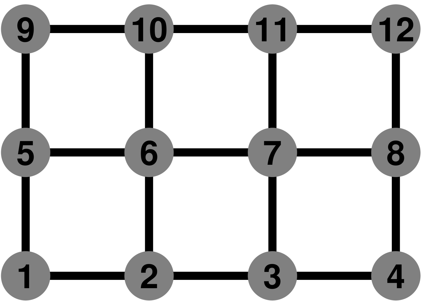
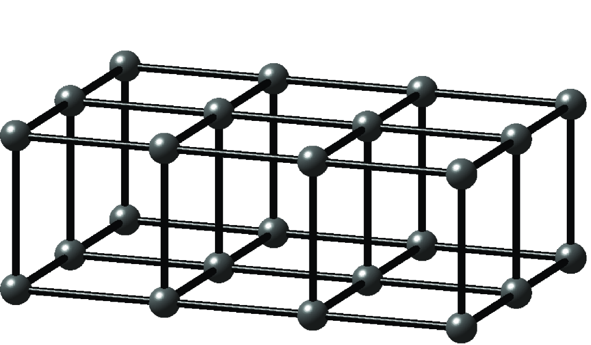
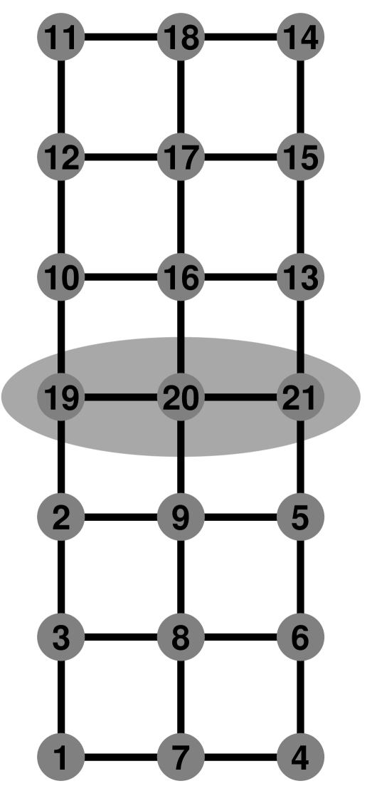
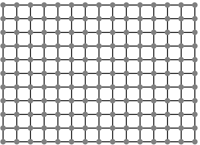
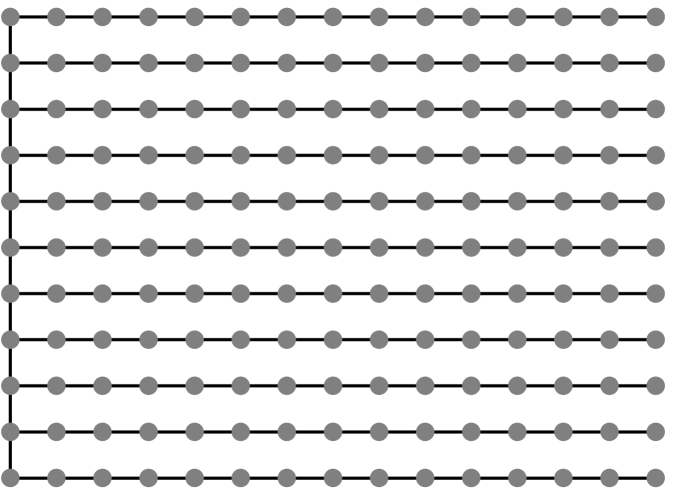
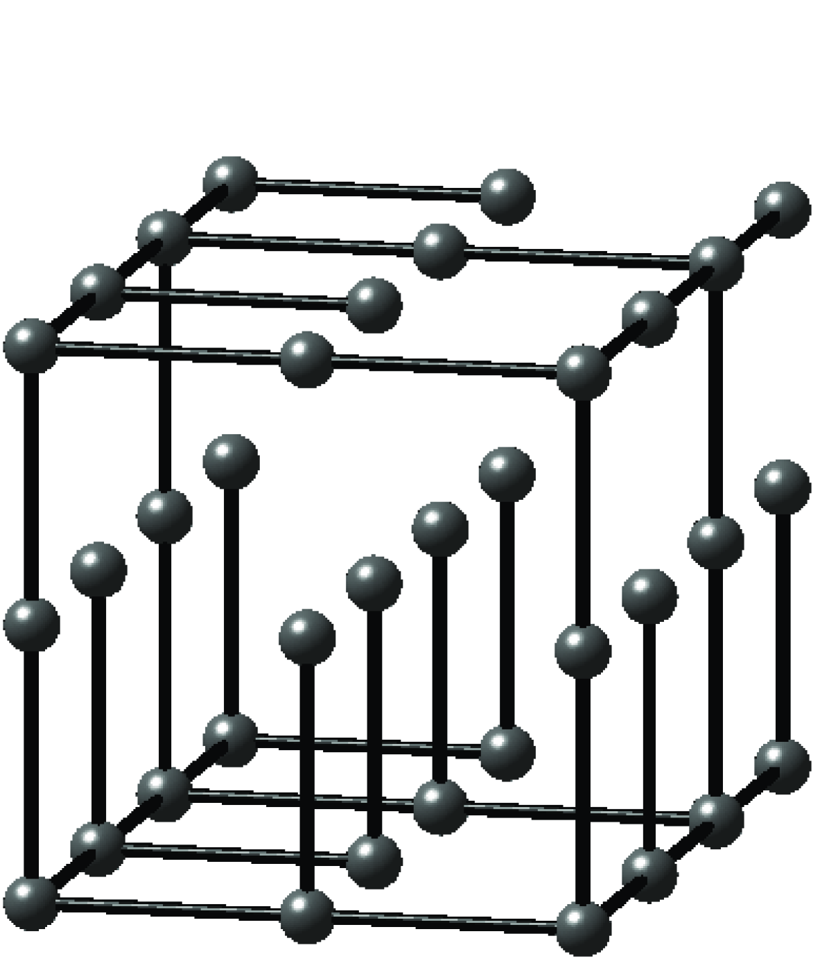
The coefficient matrices of the linear systems that we study arise from two families of undirected graphs: two- and three-dimensional meshes. The vertices of the graphs, which correspond to rows and columns in the coefficient matrix $A$ , are labeled $1$ through $n$ . The edges of the graph correspond to off-diagonal nonzeros in $A$ , the value of which is always $-1$ . If $(i,j)$ is an edge in the graph, then $A_{ij}=A_{ji}=-1$ . If $(i,j)$ is not an edge in the mesh for some $i\neq j$ , then $A_{ij}=A_{ji}=0$ . The value of the diagonal elements in $A$ is selected to make the sums of elements in rows $2,3,\ldots,n$ exactly $0$ , and to make the sum of the elements in the first row exactly $1$ . We always number meshes so that vertices that differ only in their $x$ coordinates are contiguous and numbered from small $x$ coordinates to large ones; vertices that have the same $z$ coordinate are also contiguous, numbered from small $y$ coordinates to high ones. Figure 1.1.1 shows an example of a two-dimensional mesh and the matrix that corresponds to it. Figure 1.1.2 shows an example of a small three-dimensional mesh.

Refer to caption — Figure 1.1.1. A $4$ -by- $3$ two-dimentional mesh, with vertices labeled $1,\ldots,12$ , and the coefficient matrix $A$ that corresponds to it.

Matrices similar to these do arise in applications, such as finite-difference discretizations of partial differential equations. These particular families of matrices are highly structured, and the structure allows specialized solvers to be used, such as multigrid solvers and spectral solvers. The methods that we present in this book are, however, applicable to a much wider class of matrices, not only to those arising from structured meshes. We use these matrices here only to illustrate and motivate various linear solvers.

The experimental results that we present in the rest of the chapter all use a solution vector $x$ with random uniformly-distributed elements between $0$ and $1$ .

1.2. The Cholesky Factorization

Our matrices are symmetric (by definition) and positive definite. We do not show here that they are positive definite (all their eigenvalues are positive); this will wait until a later chapter. But they are positive definite.

The simplest way to solve a linear system $Ax=b$ with a positive definite coefficient matrix $A$ is to factor $A$ into a produce of a lower triangular factor $L$ and its transpose, $A=LL^{T}$ . When $A$ is symmetric positive definite, such a factorization always exists. It is called the Cholesky factorization, and it is a variant of Gaussian Elimination. Once we compute the factorization, we can solve $Ax=b$ by solving two triangular linear systems,

	$\displaystyle Ly$	$\displaystyle=$	$\displaystyle b$
	$\displaystyle L^{T}x$	$\displaystyle=$	$\displaystyle y\;.$

Solvers for linear systems of equations that factor the coefficient matrix into a product of simpler matrices are called direct solvers. Here the factorization is into triangular matrices, but orthogonal, diagonal, tridiagonal, and block diagonal matrices are also used as factors in direct solvers.

The factorization can be computed recursively. If $A$ is $1$ -by- $1$ , then $L=\sqrt{A_{11}}$ . Otherwise, we can partition $A$ and $L$ into 4 blocks each, such that the diagonal blocks are square,

A=\begin{bmatrix}A_{11}&A_{21}^{T}\\ A_{21}&A_{22}\end{bmatrix}=\begin{bmatrix}L_{11}\\ L_{21}&L_{22}\end{bmatrix}\begin{bmatrix}L_{11}^{T}&L_{21}^{T}\\ &L_{22}^{T}\end{bmatrix}=LL^{T}\;.

This yields the following equations, which define the blocks of $L$ ,

(1.2.1)	$\displaystyle A_{11}$	$\displaystyle=$	$\displaystyle L_{11}L_{11}^{T}$
(1.2.2)	$\displaystyle A_{21}$	$\displaystyle=$	$\displaystyle L_{21}L_{11}^{T}$
(1.2.3)	$\displaystyle A_{22}$	$\displaystyle=$	$\displaystyle L_{21}L_{21}^{T}+L_{22}L_{22}^{T}\;.$

We compute $L$ by recursively solving Equation 1.2.1 for $L_{11}$ . Once we have computed $L_{11}$ , we solve Equation 1.2.2 for $L_{21}$ by substitution. The final step in the computation of $L$ is to subtract $L_{21}L_{21}^{T}$ from $A_{22}$ and to factor the difference recursively.

This algorithm is reliable and numerically stable, but if implemented naively, it is slow. Let $\phi(n)$ be the number of arithmetic operations that this algorithm performs on a matrix of size $n$ . To estimate $\phi$ , we partition $A$ so that $A_{11}$ is $1$ -by- $1$ . The partitioning does not affect $\phi(n)$ , but this particular partitioning makes it easy to estimate $\phi(n)$ . With this partitioning, computing $L$ involves computing one square root, dividing an $(n-1)$ -vector by the root, computing the symmetric outer product of the scaled $(n-1)$ -vector, subtracting this outer product from a symmetric $(n-1)$ -by- $(n-1)$ matrix, and recursively factoring the difference. We can set this up as a recurrence relation,

	$\displaystyle\phi(n)$	$\displaystyle=$	$\displaystyle 1+(n-1)+(n-1)^{2}+\phi(n-1)$
	$\displaystyle\phi(1)$	$\displaystyle=$	$\displaystyle 1\;.$

This yields

$\displaystyle\phi(n)$	$\displaystyle=$	$\displaystyle n+\sum_{j=2}^{n}(j-1)+\sum_{j=2}^{n}(n-1)^{2}$
	$\displaystyle=$	$\displaystyle n+\sum_{j=1}^{n-1}j+\sum_{j=1}^{n-1}j^{2}$
	$\displaystyle=$	$\displaystyle n+\frac{n(n-1)}{2}+\frac{n(n-\frac{1}{2})(n-1)}{3}$
	$\displaystyle=$	$\displaystyle\frac{n^{3}}{3}+o\left(n^{3}\right)\;.$

The little- $o$ notation means that we have neglected terms that grow slower than $cn^{3}$ for any constant $c$ .

Cubic growth means that for large meshes, a Cholesky-based solver is slow. For a mesh with a million vertices, the solver needs to perform more than $0.3\times 10^{18}$ arithmetic operations. Even at a rate of $10^{12}$ operations per second, the factorization takes almost 4 days. On a personal computer (say a 2005 model), the factorization will take more than a year. A mesh with a million vertices may seem like a large mesh, but it is not. The mesh has less than $2$ million edges in two dimensions and less than $3$ million in three dimensions, so its representation does not take a lot of space in memory. We can do a lot better.

1.3. Sparse Cholesky

One way to speed up the factorization is to exploit sparsity in $A$ . If we inspect the nonzero pattern of $A$ , we see that most of its elements are zero. If $A$ is derived from a 2-dimensional mesh, only 5 diagonals contain nonzero elements. If $A$ is derived from a 3-dimensional mesh, only 7 diagonals are nonzero. Figure 1.3.1 shows the nonzero pattern of such matrices. Only $O(n)$ elements out of $n^{2}$ in $A$ are nonzero.

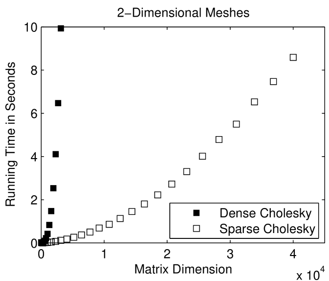
Sparse factorization codes exploit the sparsity of $A$ and avoid computations involving zero elements (except, sometimes, for zeros that are created by exact cancellations). Figure 1.3.2 compares the running times of a sparse Cholesky solver with that of a dense Cholesky solver, which does not exploit zeros. The sparse solver is clearly must faster, especially on 2-dimensional meshes.

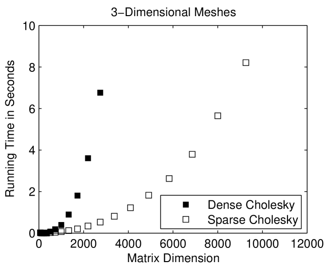
To fully understand the performance of the sparse solver, it helps to inspect the nonzero pattern of the Cholesky factor $L$ , shown in Figure 1.3.3. Exploiting sparsity pays off because the factor is also sparse: it fills, but not completely. It is easy to characterize exactly where the factor fills. It fills almost completely within the band structure of $A$ , the set of diagonals $d$ that are closer to the main diagonal than a nonzero diagonal. Outside this band structure, the elements of $L$ are all zero. For a $\sqrt{n}$ -by- $\sqrt{n}$ mesh, the outer diagonal is $\sqrt{n}$ , so the total amount of arithmetic in a sparse factorization is $n\cdot 2\left(\sqrt{n}\right)^{2}+o(n^{2})=2n^{2}+o(n^{2})$ . For large $n$ , this is a lot less than the dense $n^{3}/3+o(n^{2})$ bound. For three dimensional meshs, exploiting sparsity helps, but not as much. In a matrix corresponding to a $\sqrt[3]{n}$ -by- $\sqrt[3]{n}$ -by- $\sqrt[3]{n}$ mesh, the outer nonzero diagonal is $n^{2/3}$ , so the amount of arithmetic is $2n^{7/3}+o(n^{7/3})$ .

1.4. Preordering for Sparsity

Sparse factorization codes exploit zero elements in the reduced matrices and the factors. It turns out that by reordering the rows and columns of a matrix we can reduce fill in the reduced matrices and the factors. The most striking example for this phenomenon is the arrow matrix,

A=\begin{bmatrix}n+1&-1&-1&-1&\cdots&-1\\ -1&1\\ -1&&1\\ -1&&&1\\ \vdots&&&&\ddots\\ -1&&&&&1\end{bmatrix}\;.

When we factor this matrix, it fills completely after the elimination of the first column, since the outer product $L_{2\colon n,1}L_{2\colon n,1}^{T}$ is full (has no zeros). But if we reverse the order of the rows and columns, we have

	$\displaystyle PAP^{T}$	$\displaystyle=$	$\displaystyle\left[\begin{smallmatrix}&&&&&1\\ &&&&1\\ &&&1\\ &&1\\ &\cdot\\ 1\end{smallmatrix}\right]\left[\begin{smallmatrix}n+1&-1&-1&-1&\cdots&-1\\ -1&1\\ -1&&1\\ -1&&&1\\ \vdots&&&&\ddots\\ -1&&&&&1\end{smallmatrix}\right]\left[\begin{smallmatrix}&&&&&1\\ &&&&1\\ &&&1\\ &&1\\ &\cdot\\ 1\end{smallmatrix}\right]$
		$\displaystyle=$	$\displaystyle\left[\begin{smallmatrix}1&&&&&-1\\ &1&&&&-1\\ &&1&&&-1\\ &&&1&&-1\\ &&&&\ddots&\vdots\\ -1&-1&-1&-1&-1&n+1\end{smallmatrix}\right]\;.$

The Cholesky factor of $PAP^{T}$ is as sparse as $PAP^{T}$

\textrm{chol}(PAP^{T})=\begin{bmatrix}1\\ &1\\ &&1\\ &&&1\\ &&&&\ddots\\ -1&-1&-1&-1&\cdots&1\end{bmatrix}\;.

Solving a linear system with a Cholesky factorization of a permuted coefficient matrix is trivial. We apply the same permutation to the right-hand-side $b$ before the two triangular solves, and apply the inverse permutation after the triangular solves.

For matrices that correspond to meshes, there is no permutation that leads to a no-fill factorization, but there are permutations that reduce fill significantly. Figure 1.4.1 shows a theoretically-effictive fill-reducing permutation of the matrix of an $11$ -by- $15$ mesh and its Cholesky factor. This symmetric reordering of the rows and columns is called a nested dissection ordering. It reorders the rows and columns by finding a small set of vertices in the mesh whose removal breaks the mesh into two separate components of roughly the same size. This set is called a vertex separator and the corresponding rows and columns are ordered last. The rows and columns corresponding to each connected component of the mesh minus the separator are ordered using the same strategy recursively. Figure 1.4.2 illustrates this construction.

The factorization of the nested-dissection-ordered matrix of a a $\sqrt{n}$ -by- $\sqrt{n}$ mesh performs $\Theta(n^{3/2})$ arithmetic operations.¹¹1explain asymptotic notation. (We don’t give here the detailed analysis of fill and work under nested-dissection orderings.) For large meshes, this is a significant improvement over the $\Theta(n^{2})$ operations that the factorization performs without reordering. For a $\sqrt[3]{n}$ -by- $\sqrt[3]{n}$ -by- $\sqrt[3]{n}$ mesh, the factorization performs $\Theta(n^{2})$ operations. This is again an improvement, but the $\Theta(n^{2})$ solution cost is too high for many applications.

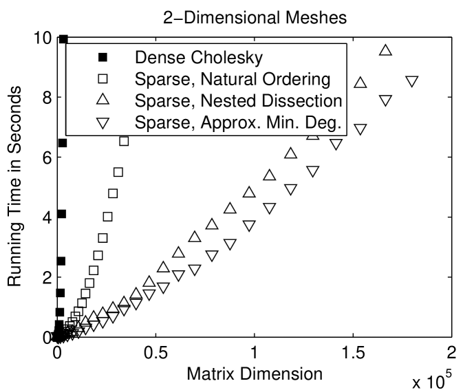
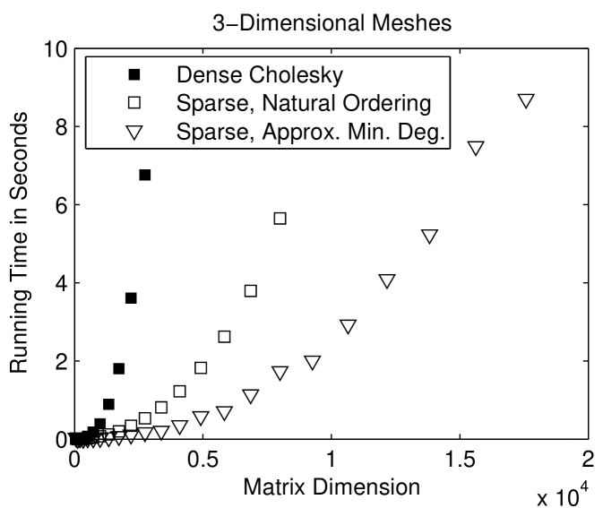
Figure 1.4.3 compares the running times of sparse Choesky applied to the natural ordering of the meshes and to fill-reducing orderings. The nested-dissection and minimum-degree orderings speed up the factorization considerably.

Unfortunately, nested-dissection-type orderings are usually the best we can do in terms of fill and work in sparse factorization of meshes, both structured and unstructured ones. A class of ordering heuristics called minimum-degree heuristics can beat nested dissection on small and medium-size meshes. On larger meshes, various hybrids of nested-dissection and minimum-degree are often more effective than pure variants of either method, but these hybrids have the same asymptotic behavior as pure nested-dissection orderings.

To asymptotically beat sparse Cholesky factorizations, we something more sophisticated than a factorization of the coefficient matrix.

1.5. Krylov-Subspace Iterative Methods

A radically different way to solve $Ax=b$ is to to find the vector $x^{(k)}$ that minimizes $\|Ax^{(k)}-b\|$ in a subspace of $\mathbb{R}^{n}$ , the subspace that is spanned by $b,Ab,A^{2}b,\ldots,A^{k-1}b$ . This subspace is called the Krylov subspace of $A$ and $b$ , and such solvers are called Krylov-subspace solvers. This idea is appealing because of two reasons, the first obvious and the other less so. First, we can create a basis for this subspace by repeatedly multiplying vectors by $A$ . Since our matrices, as well as many of the matrices that arise in practice, are so sparse, multiplying $A$ by a vector is cheap. Second, it turns out that when $A$ is symmetric, finding the minimizer $x^{(k)}$ is also cheap. These considerations, taken together, imply that the work performed by such solvers is proportional to $k$ . If $x^{(k)}$ converges quickly to $x$ , the total solution cost is low. But for most real-world problems, as well as for our meshes, convergence is slow.

The conjugate gradients method (cg) and the minimal-residual method (minres) are two Krylov-subspace methods that are appropriate for symmetric positive-definite matrices. Minres is more theoretically appealing, because it minimizes the residual $Ax^{(k)}-b$ in the $2$ -norm. It works even if $A$ is indefinite. Its main drawback is that it suffers from a certain numerically instability when implemented in floating point. The instability is almost always mild, not catastrophic, but it can slow convergence and it can prevent the method from converging to very small residuals. Conjugate gradients is more reliable numerically, but it minimizes the residual in the $A$ -norm, not in the $2$ -norm.

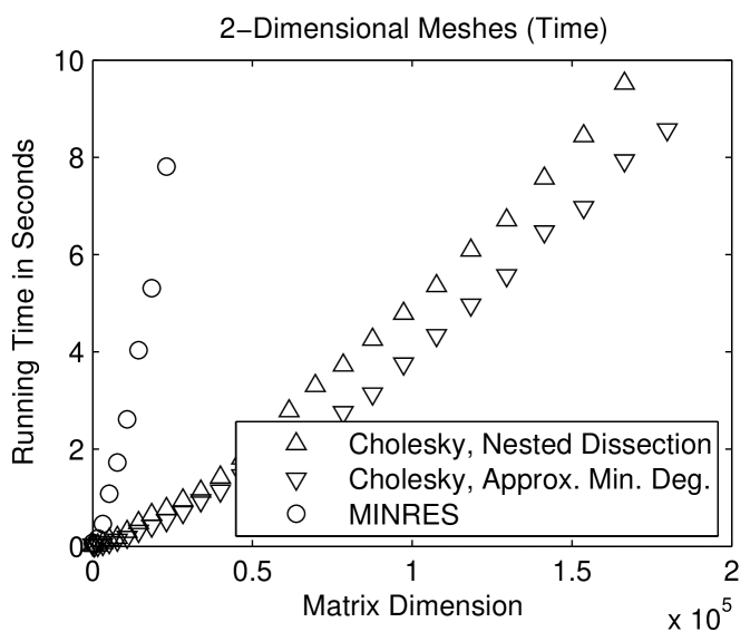
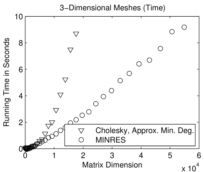
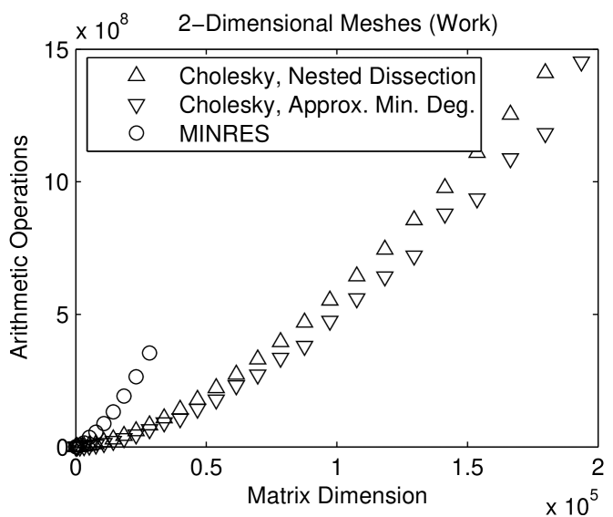
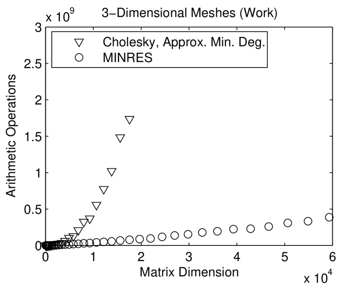
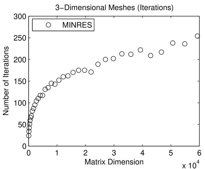
Figure 1.5.1 compares the performance of a sparse direct solver (with a fill-reducing ordering) with the performance of a minres solver. The performance of an iterative solver depends on the prescribed convergence threshold. Here we instructed the solver to halt once the relative norm of the residual

\frac{\|Ax^{(k)}-b\|}{\|b\|}

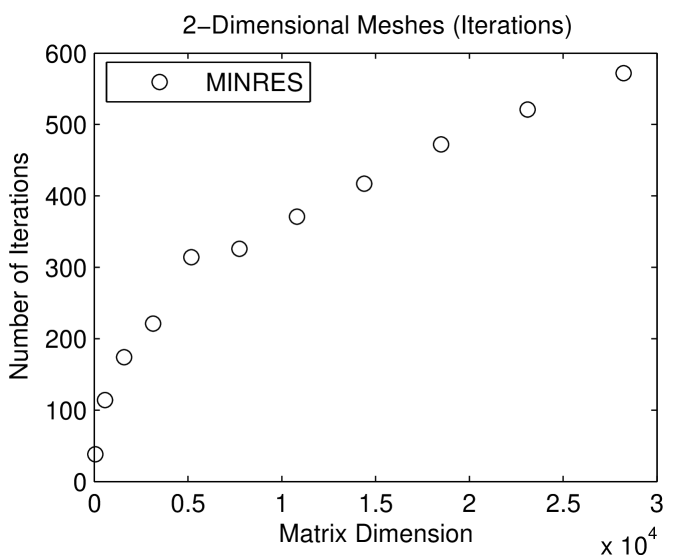
is $10^{-6}$ or smaller. On 2-dimensional meshes, the direct solver is faster. On 3-dimensional meshes, the iterative solver is faster. The fundamental reason for the difference is the size of the smallest balanced vertex separators in 2- and 3-dimensional meshes. In a 2-dimensional mesh with a bounded aspect ratio, the smallest balanced vertex separator has $\Theta(n^{1/2})$ vertices; in a 3-dimensional mesh, the size of the smallest separator is $\Theta(n^{2/3})$ . The larger separators in 3-dimensional meshes cause the direct solver to be expensive, but they speed up the iterative solver. This is shown in Figure 1.5.2: minres converges after fewer iterations on 2-dimensional meshes than on 3-dimensional meshes. The full explanation of this behavior is beyond the scope of this chapter, but this phenomenon shows how different direct and iterative solvers are. Something that hurts a direct solver may help an iterative solver.

As long as $A$ is symmetric and positive definite, the performance of a sparse Cholesky solver does not depend on the values of the nonzero elements of $A$ , only on $A$ ’s nonzero pattern. The performance of an iterative solver, on the other hand, depends on the values of the nonzero elements. The behavior of minres displayed in Figures 1.5.1 and 1.5.2 depend on our way of assigning values to nonzero elements of $A$ .

Comparing the running times of sparse and iterative solvers does not reveal all the differences between them. The graphs that present the number of arithmetic operations, in Figure 1.5.1, reveal another aspect. The differences in the amount of work that the solvers perform are much greater than the differences in running times. This indicates that the direct solver performs arithmetic at a much higher rate than the iterative solver. The exact arithmetic-rate ratio is implementation dependent, but qualitatively, direct solvers usually run at higher computational rates than iterative solvers. Most of the difference is due to the fact that it is easier to exploit complex computer architectures, in particular cache memories, in direct solvers.

Another important difference between direct and iterative solvers is memory usage. A solver like minres only allocates a few $n$ -vectors. A direct solver needs more memory, because, as we have seen, the factors fill. The Cholesky factor of a 3-dimensional mesh contains $\Omega(n^{4/3})$ nonzeros, so the memory-usage ratio between a direct and iterative solver worsens as the mesh grows.

1.6. Preconditioning

How can we improve the speed of Krylov-subspace iterative solvers? We cannot significantly reduce the cost of each iteration, because for matrices as sparse as ours, the cost of each iteration is only $\Theta(n)$ . There is little hope for finding a better approximation $x^{(k)}$ in the span of $b,Ab,\ldots,A^{k-1}b$ , because minres already finds the approximation that minimizes the norm of the residual.

To understand what can be improved, we examine simpler iterative methods. Given an approximate solution $x^{(k)}$ to the system $Ax=b$ , we define the error $e^{(k)}=x-x^{(k)}$ and the residual $r^{(k)}=b-Ax^{(k)}$ . The error $e^{(k)}$ is the required correction to $x^{(k)}$ ; if we add $e^{(k)}$ to $x^{(k)}$ , we obtain $x$ . We obviously do not know what $e^{(k)}$ is, but we know what $Ae^{(k)}$ is: it is $r^{(k)}$ , because

$\displaystyle Ae^{(k)}$	$\displaystyle=$	$\displaystyle A\left(x-x^{(k)}\right)$
	$\displaystyle=$	$\displaystyle Ax-Ax^{(k)}$
	$\displaystyle=$	$\displaystyle b-Ax^{(k)}$
	$\displaystyle=$	$\displaystyle r^{(k)}\;.$

Computing the correction requires solving a linear system of equation whose coefficient matrix is $A$ , which is what we are trying to do in the first place. The situation seems cyclic, but it is not. The key idea is to realize that even an inexact correction can bring us closer to $x$ . Suppose that we had another matrix $B$ that is close to $A$ and such that linear systems of the form $Bz=r$ are much earsier to solve than systems whose coefficient matrix is $A$ . Then we could solve $Bz^{(k)}=r^{(k)}$ for a correction $z^{(k)}$ and set $x^{(k+1)}=x^{(k)}+z^{(k)}=x^{(k)}+B^{-1}(b-Ax^{(k)})$ . Since $Ae^{(k)}=b-Ax^{(k)}$ , we can express $e^{(k)}$ directly in terms of $e^{(0)}$ ,

$\displaystyle e^{(k+1)}$	$\displaystyle=$	$\displaystyle x-x^{(k+1)}$
	$\displaystyle=$	$\displaystyle x-x^{(k)}+B^{-1}\left(b-Ax^{(k)}\right)$
	$\displaystyle=$	$\displaystyle e^{(k)}+B^{-1}Ae^{(k)}$
	$\displaystyle=$	$\displaystyle\left(I-B^{-1}A\right)e^{(k)}$
	$\displaystyle=$	$\displaystyle\left(I-B^{-1}A\right)^{k}e^{(0)}\;.$

Therefore, if $\left(I-B^{-1}A\right)^{k}$ converges quickly to a zero matrix, then $x^{(k)}$ quickly towards $x$ . This is the precise sense in which $B$ must be close to $A$ : $\left(I-B^{-1}A\right)^{k}$ should converge quickly to zero. This happens if the spectral radius of $\left(I-B^{-1}A\right)$ is small (the spectral radius of a matrix is the maximal absolute value of its eigenvalues).

The convergence of more sophisticaded iterative methods, like minres and cg, can also be accelerated using this technique, called preconditioning. In every iteration, we solve a correction equation $Bz^{(k)}=r^{(k)}$ . The coefficient matrix $B$ of the correction equation is called a preconditioner. The convergence of preconditioned minres and preconditioned cg also depends on spectral (eigenvalue) properties associated with $A$ and $B$ . For these methods, it is not the spectral radius that determines the convergence rate, but other spectral properties. But the principle is the same: $B$ should be close to $A$ in some spectral metric.

In this book, we mainly focus on one family of methods to construct and analyze preconditioners. There are many other ways. The constructions that we present are called support preconditioners, and our analysis method is called support theory.

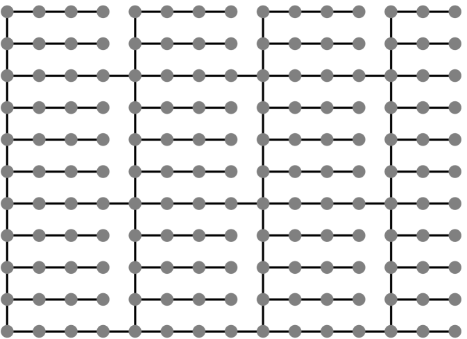
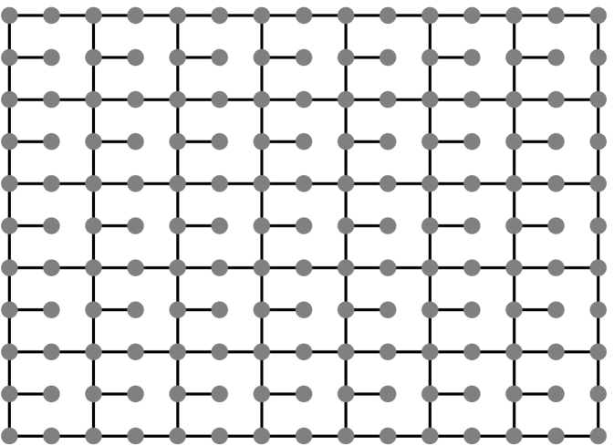
We introduce support preconditioning here using one particular family of support preconditioners for our meshes. These preconditioners, which are only effective for regular meshes whose edges all have the same weights (off-diagonals in $A$ all have the same value), are called Joshi preconditioners. We construct a Joshi preconditioner $B$ for a mesh matrix $A$ by dropping certain edges from the mesh, and then constructing a coefficient matrix $B$ for the sparsified mesh using the procedure given in Section 1.1. Figures 1.6.1 and 1.6.2 present examples of such sparsified meshes.

To solve the correction equations during the iterations, we compute the sparse Cholesky factorization of $PBP^{T}$ , where $P$ is a fill-reducing permutation $P$ for $B$ .

The construction of Joshi preconditioners depends on a parameter $k$ . For small $k$ , the mesh of the preconditioner is similar to the mesh of $A$ . In particular, for $k=1$ we obtain $B=A$ . As we shall see, Joshi preconditioners with a small $k$ lead to fast convergence rates. But Joshi preconditioners with a small $k$ do not have small balanced vertex separators, so their Cholesky factorization suffers from significant fill. Not as much as in the Cholesky factor of $A$ , but still significant. This fill slows down the preconditioner-construction phase of the linear solver, in which we construct and factor $B$ , and it also slows down each iteration. As $k$ gets larger, the similarity between the meshes diminishes. Convergence rates are worse than for small $k$ , but the factorization of $B$ and the solution of the correction equation in each iteration become cheaper. In particular, when $k$ is at least as large as the side of the mesh, the mesh of $B$ is a tree, which has single-vertex balanced separators; factoring it costs only $\Theta(n)$ operations, and its factor contains only $\Theta(n)$ nonzeros.

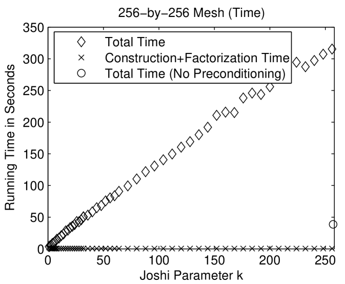
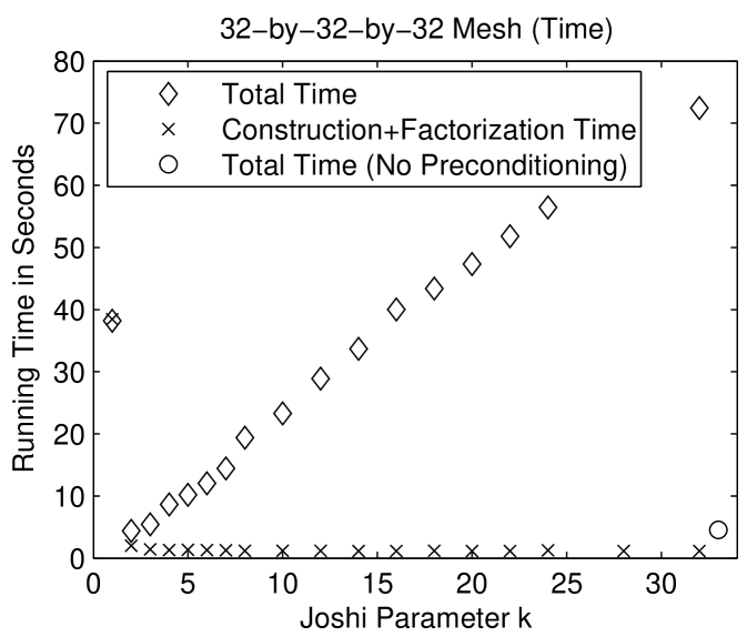
Figure 1.6.3 presents the performance of preconditioned minres with Joshi preconditioners on two meshes. On the three dimensional mesh, the preconditioned iterative solver is much faster than the direct solver and about as fast as the unpreconditioned minres solver. The preconditioned solver performs fewer arithmetic operations than both the direct solver and the unpreconditioned solver. In terms of arithmetic operations, the Joshi preconditioner for $k=3$ is the most efficient. For small $k$ , the preconditioned solvers perform fewer iterations than the unpreconditioned solver. The number of iteration rises with $k$ . Perhaps the most interesting aspect of these graphs is the fact that the cost of the factorization of $B$ drops dramatically from $k=1$ , where $B=A$ , to $k=2$ . Even slightly sparsifying the mesh reduces the cost of the factorization dramatically. The behavior on the 2-dimensional mesh is similar, except that in terms of time, the cost of the solver rises monotonically with $k$ . In particular, the direct solver is fastest. But in terms of arithmetic operations, the preconditioned solver with $k=2$ is the most efficient.

1.7. The Main Questions

We have now set the stage to pose the main questions in support theory and preconditioning. The main theme in support preconditioning is the construction of preconditioners using graph algorithms. Given a matrix $A$ , we model it as a graph $G_{A}$ . From the $G_{A}$ we build another graph $G_{B}$ , which approximates $G_{A}$ in some graph-related metric. From $G_{B}$ we build the preconditioner $B$ . The preconditioner is usually factored as preparation for solving correction equations $Bz=r$ , but sometimes the correction equation is also solved iteratively. This raises three questions

(1)

How do we model matrices as graphs?
(2)

Given two matrices $A$ and $B$ and their associated graphs $G_{A}$ and $G_{B}$ , how do we use the graphs to estimate or bound the convergence of iterative linear solvers in which $B$ preconditions $A$ ?
(3)

Given the graph $G_{A}$ of a matrix $A$ , how do we construct a graph $G_{B}$ in a metric that ensures fast convergence rates?

Support theory addresses all three questions: the modeling question, the analysis qustion, and the graph-approximation question.

The correspondence between graphs and matrices is usually an isomorphism, to allow the analysis to yield useful convergence-rate bounds. It may seem useless to transform one problem, the matrix-approximation probem, into a completely equivalent one, a graph-approximation question. It turns out, however, that many effective constructions only make sense when the problem is described in terms of graphs. They would not have been invented as matrix constructions. The Joshi preconditioners are a good example. They are highly structured when viewed as graph constructions, but would make little sense as direct sparse-matrix constructions. The analysis, on the other hand, is easier, more natural, and more general when carried out in terms of matrices. And so we transform the orignal matrix to a graph to allow for sophisticaed constructions, and then we transform the graphs back to matrices to analyze the convergence rate.

The preconditioning framework that we presented is the main theme of support theory, but there are other themes. The combinatorial and algebraic tools that were invented in order to develop preconditioners have also been used to analyze earlier preconditioners, to bound the extreme eigenvalues of matrices, to analyze the null spaces of matrices, and more.

Chapter 2 Iterative Krylov-Subspace Solvers

Preconditioned Krylov-subspace iterations are a key ingredient in many modern linear solvers, including in solvers that employ support preconditioners. This chapter presents Krylov-subspace iterations for symmetric semidefinite matrices. In particular, we analyze the convergence behavior of these solvers. Understanding what determines the convergence rate is key to designing effective preconditioners.

2.1. The Minimal Residual Method

The minimal-residual method (minres) is an iterative algorithm that finds in each iteration the vector $x^{(t)}$ that minimizes the residual $\|Ax^{(t)}-b\|_{2}$ in a subspace $\mathcal{K}_{t}$ of $\mathbb{R}^{n}$ . These subspaces, called the Krylov subspaces, are nested, $\mathcal{K}_{t}\subseteq\mathcal{K}_{t+1}$ , and the dimension of the subspace usually grows by one in every iteration, so the accuracy of the approximate solution $x^{(t)}$ tends to improve from one iteration to the next. The construction of the spaces $\mathcal{K}_{t}$ is designed to allow an efficient computation of the approximate solution in every iteration.

Definition 1.

The Krylov subspace $\mathcal{K}_{t}$ is the subspace that is spanned by the columns of the matrix $K_{t}=\begin{bmatrix}b&Ab&A^{2}b&\cdots&A^{t-1}\end{bmatrix}$ . That is,

\mathcal{K}_{t}=\left\{K_{t}y:y\in\mathbb{R}^{t}\right\}\;.

Once we have a basis for $\mathcal{K}_{t}$ , we can express the minimization of $\|Ax-b\|_{2}$ in $\mathcal{K}_{t}$ as an unconstrained linear least-squares problem, since

\min_{x\in\mathcal{K}_{t}}\|Ax-b\|_{2}=\min_{y\in\mathbb{R}^{t}}\|AK_{t}y-b\|_{2}\;.

There are three fundamental tools in the solution of least squares problems with full-rank $m$ -by- $n$ coefficient matrices with $m\geq n$ . The first tool is unitary transformations. A unitary matrix $Q$ preserves the $2$ -norm of vectors, $\|Qx\|_{2}=\|x\|_{2}$ for any $x$ (a square matrix with orthonormal columns, or equivalently, a matrix such that $QQ^{*}=I$ ). This allows us to transform least squares problem into equivalent forms

(2.1.1)

\min_{x}\|Ax-b\|_{2}=\min_{y}\|QAx-Qb\|_{2}\;.

An insight about matrices that contain only zeros in rows $n+1$ through $m$ is the second tool. Consider the least squares problem

\min_{x}\left\|\begin{bmatrix}R_{1}\\ 0\end{bmatrix}x-\begin{bmatrix}b_{1}\\ b_{2}\end{bmatrix}\right\|_{2}\;.

If the coefficient matrix has full rank, then the square block $R_{1}$ must be invertible. The solution to the problem is the vector $x$ that minimizes the Euclidean distance between $\left[\begin{smallmatrix}R_{1}\\ 0\end{smallmatrix}\right]x$ and $\left[\begin{smallmatrix}b_{1}\\ b_{2}\end{smallmatrix}\right]$ is minimal. But it is clear what is this vector: $x=R_{1}^{-1}b_{1}$ . This vector yields $\left[\begin{smallmatrix}R_{1}\\ 0\end{smallmatrix}\right]x=\begin{bmatrix}b_{1}\\ 0\end{bmatrix}$ , and we clearly cannot any closer. The third tool combines the first two into an algorithm. If we factor $A$ into a product $QR$ of a unitary matrix $Q$ and an upper trapezoidal matrix $R=\begin{bmatrix}R_{1}^{*}&0\end{bmatrix}^{*}$ , which is always possible, then we can multiply the system by $Q^{*}$ to obtain

$\displaystyle\min_{x}\left\\|Ax-b\right\\|_{2}$	$\displaystyle=$	$\displaystyle\min_{x}\left\\|QRx-b\right\\|_{2}$
	$\displaystyle=$	$\displaystyle\min_{x}\left\\|Rx-Q^{*}b\right\\|_{2}$
	$\displaystyle=$	$\displaystyle\min_{x}\left\\|\begin{bmatrix}R_{1}\\ 0\end{bmatrix}x-Q*b\right\\|_{2}\;.$

We can now compute the minimizer $x$ by substitution. Furthermore, the norm of the residual is given by $\|(Q^{*}b)_{n+1\colon m}\|_{2}$ .

In principle, we could solve (2.1.1) for $y$ using a $QR$ factorization of $AK_{t}$ . Once we find $y$ , we can compute $x=K_{t}y$ . There are, however, two serious defects in this approach. First, it is inefficient, because $AK_{t}$ is dense. Second, as $t$ grows, $A^{t}b$ tends to the subspace spanned by the dominant eigenvectors of $A$ (the eigenvectors associated with the eigenvalues with maximal absolute value). This causes $K_{t}$ to become ill conditioned; for some vectors $x\in\mathcal{K}_{t}$ with $\|x\|_{2}=1$ , the vector $y$ such that $x=K_{t}y$ has huge elements. This phenomenon will happen even if we normalize the columns of $K_{t}$ to have unit norm, and it causes instabilities when the computation is carried out using floating-point arithmetic.

We need a better basis for $\mathcal{K}_{t}$ for stability, and we need to exploit the special properties of $AK_{t}$ for efficiency. Minres does both. It uses a stable basis that can be computed efficiently, and it it combines the three basic tools in a clever way to achieve efficiency.

An orthonormal basis $Q_{t}$ for $\mathcal{K}_{t}$ would work better, because for $x=Q_{t}z$ we would have $\|z\|_{2}=\|x\|_{2}$ . There are many orthonormal bases for $\mathcal{K}_{t}$ . We choose a particular basis that we can compute incrementally, one basis column in each iteration. The basis that we use consists of the columns of the $Q$ factor from the $QR$ factorization of $K_{t}=Q_{t}R_{t}$ , where $Q_{t}$ is orthonormal and $R_{t}$ is upper triangular. We compute $Q_{t}$ using Gram-Schmidt orthogonalization. The Gram-Schmidt process is not always numerically stable when carried out in floating-point arithmetic, but it is the only efficient way to compute $Q_{t}$ one column at a time.

We now show how to compute, given $Q_{t}=\begin{bmatrix}q_{1}&\cdots&q_{t}\end{bmatrix}$ , the next basis column $q_{t+1}$ . The key to the efficient computation of $q_{t+1}$ is the special relationship of the matrices $Q_{t}$ with $A$ . We assume by induction that $K_{t}=Q_{t}R_{t}$ and that $r_{t,t}\neq 0$ . If $r_{t,t}=0$ , then it is not hard to show that the exact solution $x$ is in $\mathcal{K}_{t}$ , so we would have found it in one of the previous iterations. If we reached iteration $t$ , then $x\not\in\mathcal{K}_{t}$ , so $r_{t,t}\neq 0$ . Expanding the last column of $K_{t}=Q_{t}R_{t}$ , we get

A^{t-1}b=r_{1,t}q_{1}+r_{2,t}q_{2}+\cdots+r_{t-1,t}q_{t-1}+r_{t,t}q_{t}\;.

We now isolate $q_{t}$ to obtain

q_{t}=r_{t,t}^{-1}\left(A^{t-1}b-r_{1,t}q_{1}-r_{2,t}q_{2}-\cdots-r_{t-1,t}q_{t-1}\right)\;,

Aq_{t}=r_{t,t}^{-1}\left(A^{t}b-r_{1,t}Aq_{1}-r_{2,t}Aq_{2}-\cdots-r_{t-1,t}Aq_{t-1}\right)\;.

Because $q_{t}\in\mathcal{K}_{t}$ , clearly $Aq_{t}\in\mathcal{K}_{t+1}$ . Furthermore, if we reached iteration $t+1$ , then $Aq_{t}\not\in\mathcal{K}_{t}$ , because if $Aq_{t}\in\mathcal{K}_{t}$ then $x\in\mathcal{K}_{t}$ . Therefore, we can orthogonalize $Aq_{t}$ with respect to $q_{1},\dots,q_{t}$ and normalize to obtain $q_{t+1}$

	$\displaystyle\tilde{q}_{t+1}$	$\displaystyle=$	$\displaystyle Aq_{t}-\left(q_{t}^{}Aq_{t}\right)q_{t}-\cdots-\left(q_{1}^{}Aq_{t}\right)q_{1}$
	$\displaystyle q_{t+1}$	$\displaystyle=$	$\displaystyle\tilde{q}_{t+1}/\left\\|\tilde{q}_{t+1}\right\\|_{2}\;.$

These expressions allows us not only to compute $q_{t}$ , but also to express $Aq_{t}$ as a linear combination of $q_{1},\ldots q_{t},q_{t+1}$ ,

	$\displaystyle Aq_{t}$	$\displaystyle=$	$\displaystyle\left\\|\tilde{q}_{t+1}\right\\|_{2}q_{t+1}+\left(q_{t}^{}Aq_{t}\right)q_{t}+\cdots+\left(q_{1}^{}Aq_{t}\right)q_{1}$
		$\displaystyle=$	$\displaystyle h_{t+1,t}q_{t+1}+h_{t,t}q_{t}+\cdots+h_{1,t}q_{1}\;,$

where $h_{t+1,t}=\|\tilde{q}_{t+1}\|_{2}$ , and where $h_{j,t}=q_{j}^{*}Aq_{t}$ for $j\leq t$ . The same argument also holds for $Aq_{1},\ldots,Aq_{t-1}$ , so in matrix terms,

AQ_{t}=Q_{t+1}\tilde{H_{t}}\;.

The matrix $\tilde{H}_{t}\in\mathbb{R}^{(t+1)\times t}$ is upper Hessenberg: in column $j$ , rows $j+2$ to $t+1$ are zero. If we multiply both sides of this equation from the left by $Q_{t}^{*}$ , we obtain

$\displaystyle Q_{t}^{*}AQ_{t}$	$\displaystyle=$	$\displaystyle Q_{t}^{*}Q_{t+1}\tilde{H_{t}}$
	$\displaystyle=$	$\displaystyle\left(\begin{array}[]{ccc}1\\ &\ddots\\ &&1\\ 0&\cdots&0\end{array}\right)\tilde{H_{t}}$
	$\displaystyle=$	$\displaystyle\left(\tilde{H_{t}}\right)_{1\colon t,1\colon t}\;.$

We denote the first $t$ rows of $\tilde{H_{t}}$ by $H_{t}$ to obtain

Q_{t}^{*}AQ_{t}=H_{t}\;.

Because $A$ is symmetric, $H_{t}$ must be symmetric, and hence tridiagonal. The symmetry of $H_{t}$ implies that in column $j$ of $H_{t}$ and $\tilde{H}_{t}$ , rows $1$ through $j-2$ are also zero. This is the key to the efficiency of minres and similar algorithms, because it implies that for $j\leq t-2$ , $h_{j,t}=q_{j}^{*}Aq_{t}=0$ ; we do not need to compute these inner products and we do not need to subtract $\left(q_{j}^{*}Aq_{t}\right)q_{j}$ from $Aq_{t}$ in the orthogonalization process. As we shall shortly see, we do not even need to store $q_{j}$ for $j\leq t-2$ .

Now that we have an easy-to-compute orthonormal basis for $\mathcal{K}_{t}$ , we return to our least-squares problem

$\displaystyle\min_{x\in\mathcal{K}_{t}}\\|Ax-b\\|_{2}$	$\displaystyle=$	$\displaystyle\min_{y\in\mathbb{R}^{t}}\\|AK_{t}y-b\\|_{2}$
	$\displaystyle=$	$\displaystyle\min_{z\in\mathbb{R}^{t}}\\|AQ_{t}z-b\\|_{2}$
	$\displaystyle=$	$\displaystyle\min_{z\in\mathbb{R}^{t}}\\|Q_{t+1}\tilde{H_{t}}z-b\\|_{2}\;.$

Our strategy now is to compute the minimizer $z$ from the expression in the last line. Once we compute $z$ , the minimizer $x$ in $\mathcal{K}_{t}$ is $x=Q_{t}z$ . To compute the minimizer, we use the equality

	$\displaystyle\arg\min_{z\in\mathbb{R}^{t}}\\|Q_{t+1}\tilde{H}_{t}z-b\\|_{2}$	$\displaystyle=$	$\displaystyle\arg\min_{z\in\mathbb{R}^{t}}\\|\tilde{H}_{t}z-Q_{t+1}^{*}b\\|_{2}$
		$\displaystyle=$	$\displaystyle\arg\min_{z\in\mathbb{R}^{t}}\\|\tilde{H}_{t}z-\\|b\\|_{2}e_{1}\\|_{2}\;,$

where $e_{1}$ is the first unit vector. The equality $Q_{t+1}^{*}b=\|b\|_{2}e_{1}$ holds because $Q_{t+1}$ is the orthogonal factor in the $QR$ factorization of $K_{t+1}$ , whose first column is $b$ . To solve this least-squares problem, we will use a $QR$ factorization $\tilde{H}_{t}=V_{t}U_{t}$ of $\tilde{H}_{t}$ : the minimizer $z$ is then defined by $U_{t}z=\|b\|_{2}V_{t}^{*}e_{1}$ . Because $\tilde{H}_{t}\in\mathbb{R}^{t\times t}$ is triadiagonal we can compute its $QR$ factorization with a sequence of of $t-1$ Givens rotations, where the $i$ th rotation transforms rows $i$ and $i-1$ of $\tilde{H}_{t}$ and of $\|b\|_{2}e_{1}$ . A Given rotation is a unitary matrix of the form

\begin{bmatrix}1\\ &\ddots\\ &&1\\ &&&\cos\theta&\sin\theta\\ &&&-\sin\theta&\cos\theta\\ &&&&&1\\ &&&&&&\ddots\\ &&&&&&&1\end{bmatrix}\;.

We choose $\theta$ so as to anihilate the subdiagonal element in column $i$ of $\tilde{H}_{t}$ .

One difficulty that arises is that $z=z_{t}$ changes completely in every iteration, so to form $x=Q_{t}z$ , we need to either store all the columns of $Q_{t}$ to produce the approximate solution $x$ , or to recompute $Q_{t}$ again once we obtain a $z$ that ensures a small-enough residual. Fortunately, there is a cheaper alternative that only requires storing a constant number of vectors. Let $M_{t}=Q_{t}U_{t}^{-1}$ , and let $w=U_{t}z$ . Instead of solving for $z$ , we only compute $w=\|b\|_{2}V_{t}^{*}e_{1}$ . Because the $i$ the rotation only transforms rows $i-1$ and $i$ of $\|b\|_{2}e_{1}$ , we can compute $w$ one entry at a time. Since $x=Q_{t}z=Q_{t}U_{t}^{-1}U_{t}z=M_{t}w$ , we can accumulate $x$ using the columns of $M_{t}$ . We compute the columns of $M_{t}$ one at a time using the triangular linear system $U_{t}M_{t}=Q_{t}$ ; in iteration $t$ , we compute the last column of $M_{t}$ from $U_{t}$ and the last column of $Q_{t}$ .

minres( $A,b$ )
   $q_{1}=b/\|b\|_{2}$ $\triangleright$ the first column of $Q_{t}$
   $w_{1}=\|b\|_{2}$ $\triangleright$ the first element of the vector $w$
  for $t=1,2,\ldots$ until convergence
    compute $Aq_{t}$
     $\tilde{q}_{t+1}=Aq_{t}-\left(q_{t}^{*}Aq_{t}\right)q_{t}-\left(q_{t-1}^{*}Aq_{t}\right)q_{t-1}$
     $H_{t+1,t}=\|\tilde{q}_{t+1}\|_{2}$
     $H_{t,t}=q_{t}^{*}Aq_{t}$
     $H_{t-1,t}=q_{t-1}^{*}Aq_{t}$
     $q_{t+1}=\tilde{q}_{t+1}/\left\|\tilde{q}_{t+1}\right\|_{2}$
     $\triangleright$ Apply rotation $t-2$ to $H_{\colon,t}$
     $R_{t-2,t}=s_{t-2}H_{t-1,t}$
    if $t>2$ then $U_{t-1,t}=c_{t-2}H_{t-1,t}$ else $U_{t-1,t}=H_{t-1,t}$
     $\triangleright$ Apply rotation $t-1$ to $H_{\colon,t}$
     $U_{t-1,t}=c_{t-1}U_{t-1,t}+s_{t-1}H_{t,t}$
    if $t>1$ then $U_{t,t}=-s_{t-1}U_{t-1,t}+c_{t-1}H_{t,t}$ else $U_{t,t}=H_{t,t}$
    compute $\left[\begin{smallmatrix}c_{t}&-s_{t}\\ s_{t}&c_{t}\end{smallmatrix}\right]$ , the Givens rotation such
     that $\left[\begin{smallmatrix}c_{t}&-s_{t}\\ s_{t}&c_{t}\end{smallmatrix}\right]\left[\begin{smallmatrix}U_{t,t}\\ H_{t+1,t}\end{smallmatrix}\right]=\left[\begin{smallmatrix}\textrm{anything}\\ 0\end{smallmatrix}\right]$
     $\triangleright$ Apply rotation $t$ to $H_{\colon,t}$
     $U_{t,t}=c_{t}U_{t,t}+s_{t}H_{t+1,t}$
     $\triangleright$ Apply rotation $t$ to form $w=U_{t}z=V_{t}^{*}\|b\|e_{1}$
     $w_{t+1}=-s_{t}w_{t}$
     $w_{t}=c_{t}w_{t}$
     $m_{t}=r_{t,t}^{-1}\left(q_{t}-U_{t-1,t}m_{t-1}-U_{t-2,t}m_{t-2}\right)$ $\triangleright$ next column of $M$
     $x^{(t)}=x^{(t-1)}+w_{t}m_{t}$
  end for

Figure 2.1.1. Minres. To keep the pseudo-code simple, we use the convention that vectors and matrix/vector elements with nonpositive indices are zeros. By this convension,

x^{(0)}=q_{0}=m_{0}=m_{-1}=0

, and so on. In an actual code, this convension can be implemented either using explicit zero vectors or using conditionals.

2.2. The Conjugate Gradients Algorithm

Minres is a variant of an older and more well-known algorithm called the Conjugate Gradients method (cg). The Conjugate Gradients method is only guaranteed to work when $A$ is symmetric positive definite, whereas minres only requires $A$ to be symmetric. Conjugate Gradients also minimizes the norm of the residuals over the same Krylov subspaces, but not the $2$ -norm but the $A^{-1}$ -norm,

\|Ax^{(t)}-b\|_{A^{-1}}=\sqrt{\left(Ax^{(t)}-b\right)^{*}A^{-1}\left(Ax^{(t)}-b\right)}\;.

This is equivalent to minimizing the $A$ -norm of the error,

\|x-x^{(t)}\|_{A}=\sqrt{\left(x-x^{(t)}\right)^{*}A\left(x-x^{(t)}\right)}\;.

Minimizing the $A$ -norm of the residual may seem like an odd idea, because of the dependence on $A$ in the measurement of the residual and the error. But there are several good reasons not to worry. First, we use the $2$ -norm of the residual as a stoping criterion, to stop the iterations only when the $2$ -norm is small enough, not when the $A^{-1}$ -norm is small. Second, even when the stopping criterion is based on the $2$ -norm of the residual, Conjugate Gradients usually converges only slightly slower than minres. Still, the minimization of the $2$ -norm of the residual in minres is more elegant.

Why do people use Conjugate Gradients if minres is more theoretically appealing? The main reason that that the matrices $M_{t}=Q_{t}R_{t}^{-1}$ and $R_{t}$ that are used in minres to form $x^{(t)}$ can be ill conditioned. This means that in floating-point arithmetic, the computed $x^{(t)}$ are not always accurate minimizers. In the Conjugate Gradients method, the columns of the basis matrix (the equivalent of $M_{t}$ ) are $A$ -conjugate, not arbitrary. This reduces the inaccuracies in the computation of the approximate solution in each iterations, so the method is numerically more stable than minres.

We shall not derive the details of the Conjugate Gradient method here. The derivation is similar to that of minres (there are also other ways to derive cg), and is presented in many textbooks.

2.3. Convergence-Rate Bounds

The appeal of Krylov-subspace iterations stems to some extent from the fact that their convergence is easy to understand and to bound.

The crucial step in the analysis is the expression of the residual $b-Ax^{(t)}$ as a application of a univariate polynomial $\tilde{p}$ to $A$ and a multiplication of the resulting matrix $\tilde{p}(A)$ by $b$ . Since $x^{(t)}\in\mathcal{K}_{t}$ , $x^{(t)}=K_{t}y$ for some $y$ . That is, $x^{(t)}=y_{1}b+y_{2}Ab+\cdots y_{t}A^{t-1}b$ . Therefore,

b-Ax^{(t)}=b-y_{1}Ab-y_{2}A^{2}b-\cdots-y_{t}A^{t}b\;.

If we denote $p(z)=1-y_{1}z-y_{2}z^{2}-\cdots-y_{t}z^{t}=1-z\tilde{p}(z)$ , we obtain $b-Ax^{(t)}=p(A)b$ .

Definition 2.

Let $x^{(t)}\in\mathcal{K}_{t}$ be an approximate solution of $Ax=b$ and let $r^{(t)}=b-Ax^{(t)}$ be the corresponding residual. The polynomial $\tilde{p}_{t}$ such that $x^{(t)}=\tilde{p}_{t}(A)b$ is called the solution polynomial of the iteration and the polynomial $p_{t}(z)=1-z\tilde{p}(z)$ is called the residual polynomial of the iteration.

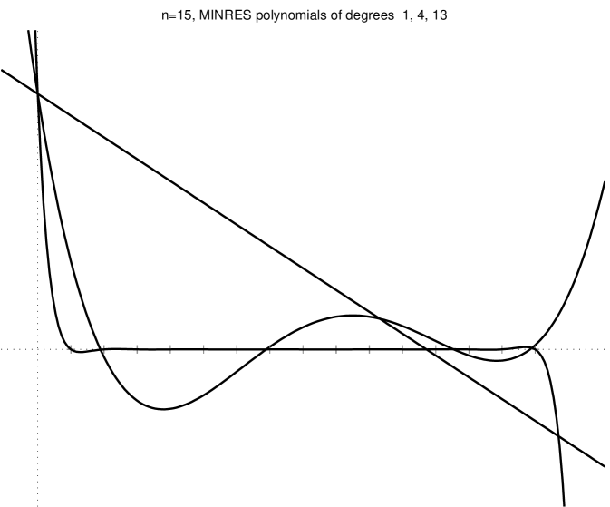
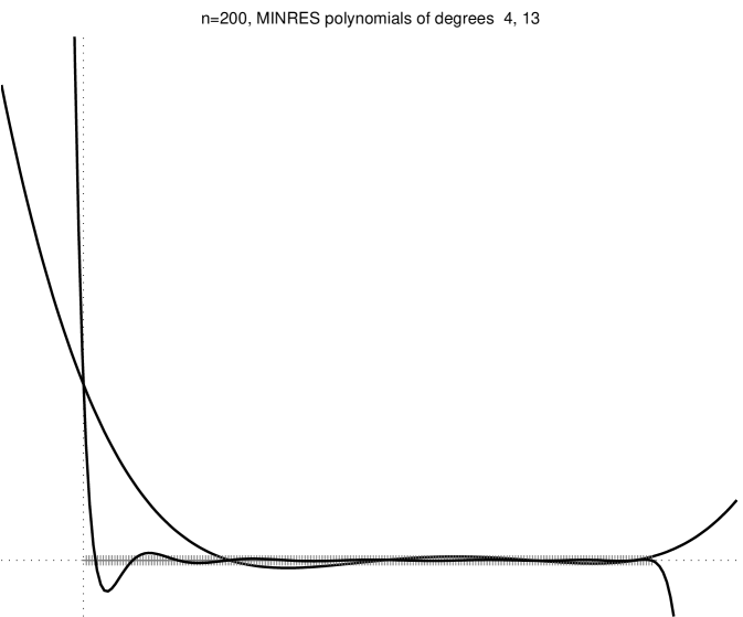
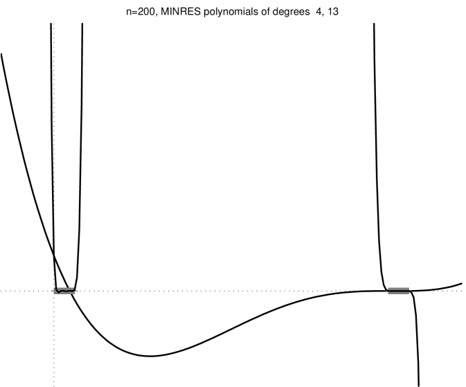
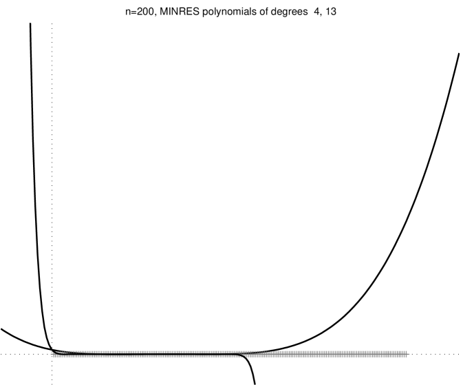
Figure 2.3.1 shows several minres residual polynomials.

We now express $p(A)$ in terms of the eigendecomposition of $A$ . Let $A=V\Lambda V^{*}$ be an eigendecomposition of $A$ . Since $A$ is Hermitian, $\Lambda$ is real and $V$ is unitary. We have

p(A)b=p\left(V\Lambda V^{*}\right)b=Vp(\Lambda)V^{*}b\;,

(2.3.1)

\left\|b-Ax^{(t)}\right\|_{2}=\left\|p(A)b\right\|_{2}=\left\|Vp(\Lambda)V^{*}b\right\|_{2}=\left\|p(\Lambda)V^{*}b\right\|_{2}\;.

We can obtain several bounds on the norm of the residual from this expression. The most important one is

$\displaystyle\left\\|b-Ax^{(t)}\right\\|_{2}$	$\displaystyle=$	$\displaystyle\left\\|p(\Lambda)V^{*}b\right\\|_{2}$
	$\displaystyle\leq$	$\displaystyle\left\\|p(\Lambda)\right\\|_{2}\left\\|V^{*}b\right\\|_{2}=\left\\|p(\Lambda)\right\\|_{2}\left\\|b\right\\|_{2}$
	$\displaystyle=$	$\displaystyle\max_{i=1}^{n}\left\{\left\|p\left(\lambda_{i}\right)\right\|\right\}\left\\|b\right\\|_{2}\;.$

The last equality follows from the facts that $p(\Lambda)$ is a diagonal matrix and that the $2$ -norm of a diagonal matrix is the largest absolute value of an element in it. This proves the following result.

Theorem 3.

The relative $2$ -norm of the residual in the $t$ th iteration of minres,

\left\|b-Ax^{(t)}\right\|_{2}/\left\|b\right\|_{2}\;,

is bounded by $\max_{i=1}^{n}\left\{\left|p\left(\lambda_{i}\right)\right|\right\}$ for any univariate polynomial $p$ of degree $t$ such that $p(0)=1$ , where the $\lambda_{i}$ ’s are the eigenvalues of $A$ .

We can strenghen this result by noting that if $b$ is a linear combination of only some of the eigenvectors of $A$ , then only the action of $p$ on corresponding eigenvalues matters (not on all the eigenvalues). An example of this behavior is shown in the bottom-right plot of Figure 2.3.1. More formally, from (2.3.1) we obtain

\left\|p(\Lambda)V^{*}b\right\|_{2}=\left\|\begin{bmatrix}p(\lambda_{1})(v_{1}^{*}b)\\ p(\lambda_{2})(v_{2}^{*}b)\\ \vdots\\ p(\lambda_{n})(v_{n}^{*}b)\end{bmatrix}\right\|_{2}\;.

In general, if $b$ is orthogonal or nearly orthogonal to an eigenvector $v_{j}$ of $A$ , then the product $p(\lambda_{j})(v_{j}^{*}b)$ can be small even if $p(\lambda_{j})$ is quite large. But since right-hand sides $b$ with this property are rare in practice, this stronger bound is not useful for us.

Theorem 3 states that if there are low-degree polynomials that are low on the eigenvalues of $A$ and assume the value $1$ at $0$ , the minres converges quickly. Let us examine a few examples. A degree- $n$ polynomial $p$ can satisfy $p(0)=1$ and $p(\lambda_{i})=0$ simulteneously for any set of $n$ nonzero eigenvalues $\lambda_{1},\ldots,\lambda_{n}$ . Therefore, in the absense of rounding errors minres must converge after $n$ iterations to the exact solution. We could also derive this exact-convergence result from the fact that $\mathcal{K}_{n}=\mathbb{R}^{n}$ , but the argument that we just gave characterizes the minres polynomials at or near convergence: their roots are at or near the eigenvalues of $A$ . If $A$ has repeated eigenvalues, then it has fewer than $n$ distinct eigenvalues, so we expect exact convergence after fewer than $n$ iterations. Even if $A$ does not have repeated eigenvalues, but it does have only a few tight clusters of eigenvalues, then minres will converge quickly, because a polynomial with one root near every cluster and a bounded derivative at the roots will assume low values at all the roots. On the other hand, a residual polynomial cannot have small values very close to $0$ , because it must assume the value $1$ at $0$ . These examples lead us to the most important observation about Krylov-subspace solvers:

Symmetric Krylov-subspace iterative methods for solving linear systems of equations $Ax=b$ converge quickly if the eigenvalues of $A$ form a few tight clusters and if $A$ does not have eigenvalues very close to $0$ .

Scaling both $A$ and $b$ can cluster the eigenvalues or move them away from zero, but has no effect at all on convergence. Scaling up $A$ and $b$ moves the eigenvalues away from zero, but distributes them on a larger interval; scaling $A$ and $b$ down clusters the eigenvalues around zero, but this brings them closer to zero. Krylov-subspace iterations are invariant to scaling.

This observation leads to two questions, one analytic and one constructive: (1) Exactly how quickly does the iteration converges given some characterization of the spectrum of $A$ ? (2) How can we alter the specturm of $A$ in order to accelerate convergence? We shall start with the second question.

2.4. Preconditioning

Suppose that we have a matrix $B$ that approximates $A$ (in a sense that will become clear shortly), and whose inverse is easier to apply than the inverse of $A$ . That is, linear systems of the form $Bz=r$ are much easier to solve for $z$ than linear systems $Ax=b$ . Perhpas the sparse Cholesky factorization of $B$ is cheaper to compute than $A$ ’s, and perhaps there is another inexpensive way to apply $B^{-1}$ to $r$ . If $B$ approximates $A$ in the sense that $B^{-1}A$ is close to the identity, then an algorithm like minres will converge quickly when applied to the linear system

(2.4.1)

\left(B^{-1}A\right)x=B^{-1}b\;,

because the eigenvalues of the coefficient matrix $B^{-1}A$ are clustered around $1$ . We will initialize the algorithm by computing the right-hand side $B^{-1}$ , and in every iteration we will multiply $q_{t}$ by $A$ and then apply $B^{-1}$ to the product. This technique is called preconditioning.

The particular form of preconditioning that we used in (2.4.1) is called left preconditioning, because the inverse of the preconditioner $B$ is applied to both sides of $Ax=b$ from the left. Left preconditioning is not appropriate to algorithms line minres and Conjugate Gradients that exploit the symmetry of the coefficient matrix, because in general $B^{-1}A$ is not symmetric. We could replace minres by a Krylov-subspace iterative solver that is applicable to unsymmetric matrices, but this would force us to give up either the efficiency or the optimality of minres and Conjugate Gradients.

Fortunately, if $B$ is symmetric positive definite, then there are forms of preconditioning that are appropriate for symmetric Krylov-subspace solvers. One form of symmetric preconditioning solves

(2.4.2)

\left(B^{-1/2}AB^{-1/2}\right)\left(B^{1/2}x\right)=B^{-1/2}b

for $x$ . A clever transformation of Conjugate Gradients yields an iterative algorithm in which the matrix that generates the Krylov subspace is $\left(B^{-1/2}AB^{-1/2}\right)$ , but which only applies $A$ and $B^{-1}$ in every iteration. In other words, $B^{-1/2}$ is never used, not even as a linear operator. We shall not show this transformation here.

We will show how to use a simpler but equally effective form of preconditioning. Let $B=LL^{T}$ be the Cholesky factorization of $A$ . We shall solve

(2.4.3)

\left(L^{-1}AL^{-T}\right)\left(L^{T}x\right)=L^{-1}b

for $y=L^{T}x$ using minres, and then we will solve $L^{T}x=y$ by substitution. To form the right-hand side $L^{-1}b$ , we solve for it by substitution as well. The coefficient matrix $L^{-1}AL^{-T}$ is clearly symmetric, so we can indeed apply minres to it. To apply the coefficient matrix to $q_{t}$ in every iteration, we apply $L^{-T}$ by substitution, apply $A$ , and apply $L^{-1}$ by substitution.

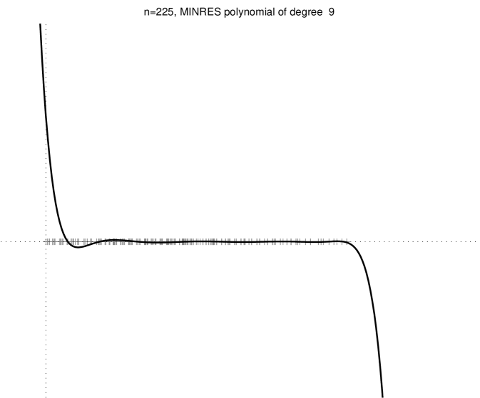Figure 2.4.1 shows the spectrum and one minres polynomial for two matrices: a two-dimensional mesh and the same mesh preconditioned as in (2.4.3) with a Joshi preconditioner $B$ . We can see that this particular preconditioner causes three changes in the spectrum. The most important change is the small eigenvalues of $L^{-1}AL^{-T}$ are much larger than the small eigenvalues of $A$ . This allows the minres polynomial to assume much smaller vaues on the spectrum. The minres polynomials must assume the value $1$ at $0$ , so they tend to have large values on the neighborhood of $0$ as well. Therefore, a specturm with larger smallest eigenvalues leads to faster convergence. Indeed, the preconditioned problem decreased the size of the residual by a factor $10^{-14}$ in $46$ iterations, whereas the unpreconditioned problem took $110$ iterations to achieve a residual with a similar norm. Two other changes that the preconditioner caused are a large gap in the middle of the spectrum, which is a good thing, and a larger largest eigenvalue, which is not. But these two changes are probably less important than the large increase in the smallest eigenvalues.

The different forms of preconditioning differ in the algorithmic details of the solver, but they all have the same spectrum.

Theorem 4.

Let $A$ be a symmetric matrix and let $B=LL^{T}$ be a symmetric positive-definite matrix. A scalar $\lambda$ is either an eigenvalue of all the following eigenvalue problems or of none of them:

$\displaystyle B^{-1}Ax$	$\displaystyle=$	$\displaystyle\lambda x$
$\displaystyle B^{-1/2}AB^{-1/2}y$	$\displaystyle=$	$\displaystyle\lambda y$
$\displaystyle L^{-1}AL^{-T}z$	$\displaystyle=$	$\displaystyle\lambda z$
$\displaystyle Aw$	$\displaystyle=$	$\displaystyle\lambda Bw$

Proof.

The following relations prove the equivalence of the specta:

$\displaystyle x$	$\displaystyle=$	$\displaystyle B^{-1/2}y$
$\displaystyle y$	$\displaystyle=$	$\displaystyle B^{1/2}x$
$\displaystyle x$	$\displaystyle=$	$\displaystyle L^{-T}z$
$\displaystyle z$	$\displaystyle=$	$\displaystyle L^{T}x$
$\displaystyle x$	$\displaystyle=$	$\displaystyle w$

∎

We can strengthen this theorem to also include certain semidefinite preconditioners.

Theorem 5.

Let $A$ be a symmetric matrix and let $B=LL^{T}$ be a symmetric positive-semidefinite matrix such that $\textrm{null}(B)=\textrm{null}(A)$ . Denote by $X^{+}$ the pseudo-inverse of a matrix $X$ . A scalar $\lambda$ is either an eigenvalue of all the following eigenvalue problems or of none of them:

$\displaystyle B^{+}Ax$	$\displaystyle=$	$\displaystyle\lambda x$
$\displaystyle\left(B^{+}\right)^{1/2}A\left(B^{+}\right)^{1/2}y$	$\displaystyle=$	$\displaystyle\lambda y$
$\displaystyle\left(L^{+}\right)A\left(L^{+}\right)^{T}z$	$\displaystyle=$	$\displaystyle\lambda z$
$\displaystyle Aw$	$\displaystyle=$	$\displaystyle\lambda Bw$

Proof.

We note that $\textrm{null}(L^{+})=\textrm{null}((L^{+})^{T})=\textrm{null}(B^{+})=\textrm{null}(B)=\textrm{null}(A)$ . Therefore, $\lambda=0$ is an eigenvalue of all the above problems. If $\lambda\neq 0$ is an eigenvalue of one of the above problems, then the corresponding eigenvector is not in $\textrm{null}(A)$ . This implies that the relations defined in the proof of Theorem 4, with inverses replaced by pseudo-inverses, define relations between nonzero vectors. Therefore, $\lambda$ is an eigenvalue of all the eigenvalue problems. ∎

Even though the different forms of preconditioning are equivalent in terms of the spectra of the coefficient matrices, they are different algorithmically. If symmetry is not an issue (e.g., if $A$ itself is unsymmetric), the form $B^{-1}A$ is the most general. When $A$ is symmetric, we usually require that $B$ is symmetric positive-definite (or semi-definite with the same null space as $A$ ). In this case, the form $B^{-1/2}AB^{-1/2}$ , when coupled with the transformation that allows multiplications only by $B^{-1}$ (and not by $B^{-1/2}$ ), is more widely applicable than the form $L^{-1}AL^{-T}$ , because the latter requires a Cholesky factorization of $B$ , whereas in the former any method of applying $B^{-1}$ can be used.

One issue that arizes with any form of preconditioning is the definition of the residual. If we apply minres to $\left(L^{-1}AL^{-T}\right)\left(L^{T}x\right)=L^{-1}b$ , say, it minimizes the $2$ -norm of the preconditioned residual

L^{-1}b-\left(L^{-1}AL^{-T}\right)\left(L^{T}x^{(t)}\right)=L^{-1}b-L^{-1}Ax^{(t)}=L^{-1}\left(b-Ax^{(t)}\right)\;.

Thus, the true residual $b-Ax^{(t)}$ in preconditioned minres may not be minimal. This is roughly the same issue as with the norms used in Conjugate Gradients: we minimize the residual in a norm that is related to $A$ .

2.5. Chebyshev Polynomials and Convergence Bounds

The link between Krylov-subspace iterations and polynomials suggests another idea. Given some information on the spectrum of $A$ , we can try to analytically define a sequence $\tilde{p}_{t}$ of solution polynomials such that for any $b$ the vector $x^{(t)}\equiv\tilde{p}_{t}(A)b\in\mathcal{K}_{t}$ is a good approximation to $x$ , the exact solution of $Ax=b$ . More specifically, we can try to define $\tilde{p}_{t}$ such that the residuals $b-Ax^{(t)}$ are small. We have seen that the residual can be expressed as $p_{t}(A)b$ , where $p_{t}(z)=1-z\tilde{p}_{t}(z)$ is the residual polynomial. Therefore, if $\tilde{p}_{t}$ is such that $p_{t}$ assumes low values on the eigenvalues of $A$ and satisfies $p_{t}(0)=1$ , then $x^{(t)}$ is a good approximate solution. This idea can be used both to construct iterative solvers and to prove bounds on the convergence of methods like minres and Conjugate Gradients.

One obvious problem is that we do not know what the eigenvalues of $A$ are. Finding the eigenvalues is more difficult than solving $Ax=b$ . However, in some cases we can use the structure of $A$ (even with preconditioning) to derive bounds on the smallest and largest eigenvalues of a positive-definite martrix $A$ , denoted $\lambda_{\min}$ and $\lambda_{\max}$ .

Suppose that we somehow obtained bounds on the extereme eigenvalues of $A$ ,

0<\rho_{\min}\leq\lambda_{\min}\leq\lambda_{i}\leq\lambda_{\max}\leq\rho_{\max}\;.

We shall not discuss here how we might obtain $\rho_{\min}$ and $\rho_{\max}$ ; this is the topic of much of the rest of the book. It turns out that we can build a sequence $p_{t}$ of polynomials such that

(1)

$p_{t}(0)=1$ , and
(2)

$\max_{z\in[\rho_{\min},\rho_{\max}]}\left|p_{t}(z)\right|$ is as small as possible for a degree $t$ polynomial with value $1$ at $0$ .

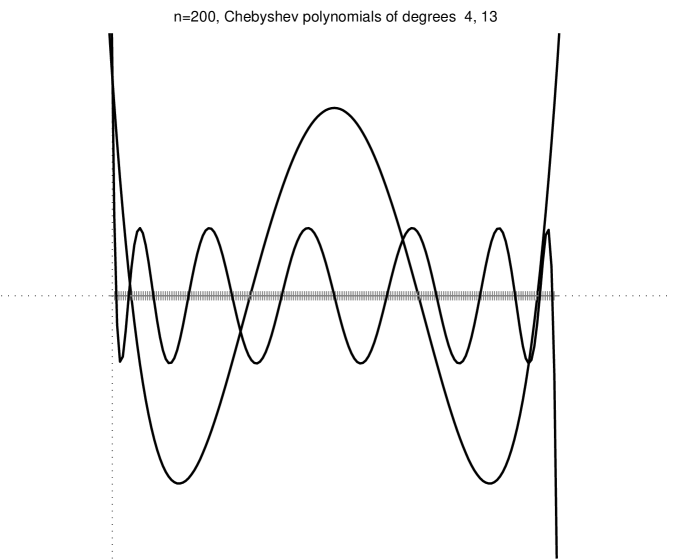
The polynomials that solve this optimization problem are derived from Chebyshev polynomials, which can be defined using the recurrence

$\displaystyle c_{0}(z)$	$\displaystyle=$	$\displaystyle 1$
$\displaystyle c_{1}(z)$	$\displaystyle=$	$\displaystyle z$
$\displaystyle c_{t}(z)$	$\displaystyle=$	$\displaystyle 2zc_{t-1}(z)-c_{t-2}(z)\;.$

The polynomials that reduce the residual are

p_{t}(z)=\frac{1}{c_{t}\left(\frac{\rho_{\max}+\rho_{\min}}{\rho_{\max}-\rho_{\min}}\right)}c_{t}\left(\frac{\rho_{\max}+\rho_{\min}-2z}{\rho_{\max}-\rho_{\min}}\right)\;.

An Iterative Linear Solver based on Chebyshev Polynomials

Our first application of Chebyshev polynomials is an iterative Krylov-subspace solver based on them. We will refer to this solver as the Krylov-Chebyshev solver¹¹1The algorithm that we describe below is related to a more well-known Chebychev linear solver that is used with matrix splittings.. The polynomials $p_{t}$ implicitly define polynomials $\tilde{p}_{t}$ that we can use to construct approximate solutions. The residual for an approximate solution $x^{(t)}$ is $r^{(t)}=b-Ax^{(t)}$ . If we define $x^{(t)}=\tilde{p}_{t}(A)b$ , we have $r^{(t)}=p_{t}(A)b=b-A\tilde{p}_{t}(A)b$ .

We now derive recurrences for $x^{(t)}$ and $r^{(t)}$ . To keep the notation simple, we define $\rho_{+}=\rho_{\max}+\rho_{\min}$ and $\rho_{-}=\rho_{\max}+\rho_{\min}$ . For the two base cases we have

$\displaystyle r^{(0)}=p_{0}(A)b$	$\displaystyle=$	$\displaystyle c_{0}^{-1}\left(\frac{\rho_{+}}{\rho_{-}}\right)c_{0}\left(\frac{\rho_{+}}{\rho_{-}}I-\frac{2}{\rho_{-}}A\right)b=Ib=b$
$\displaystyle r^{(1)}=p_{1}(A)b$	$\displaystyle=$	$\displaystyle c_{1}^{-1}\left(\frac{\rho_{+}}{\rho_{-}}\right)c_{1}\left(\frac{\rho_{+}}{\rho_{-}}I-\frac{2}{\rho_{-}}A\right)b$
	$\displaystyle=$	$\displaystyle\left(\frac{\rho_{+}}{\rho_{-}}\right)^{-1}\left(\frac{\rho_{+}}{\rho_{-}}I-\frac{2}{\rho_{-}}A\right)b=b-\frac{2}{\rho_{+}}Ab\;.$

This implies that

	$\displaystyle x^{(0)}$	$\displaystyle=$	$\displaystyle 0$
	$\displaystyle x^{(1)}$	$\displaystyle=$	$\displaystyle\frac{2}{\rho_{+}}b\;.$

For $t\geq 2$ we have

$\displaystyle p_{t}(A)b$	$\displaystyle=$	$\displaystyle c_{t}^{-1}\left(\frac{\rho_{+}}{\rho_{-}}\right)c_{t}\left(\frac{\rho_{+}}{\rho_{-}}I-\frac{2}{\rho_{-}}A\right)b$
	$\displaystyle=$	$\displaystyle c_{t}^{-1}\left(\frac{\rho_{+}}{\rho_{-}}\right)\left(2\left(\frac{\rho_{+}}{\rho_{-}}I-\frac{2}{\rho_{-}}A\right)c_{t-1}\left(\frac{\rho_{+}}{\rho_{-}}I-\frac{2}{\rho_{-}}A\right)-c_{t-2}\left(\frac{\rho_{+}}{\rho_{-}}I-\frac{2}{\rho_{-}}A\right)\right)b$
	$\displaystyle=$	$\displaystyle c_{t}^{-1}\left(\frac{\rho_{+}}{\rho_{-}}\right)\left(2\left(\frac{\rho_{+}}{\rho_{-}}I-\frac{2}{\rho_{-}}A\right)c_{t-1}\left(\frac{\rho_{+}}{\rho_{-}}\right)p_{t-1}\left(A\right)-c_{t-2}\left(\frac{\rho_{+}}{\rho_{-}}\right)p_{t-2}\left(A\right)\right)b$
	$\displaystyle=$	$\displaystyle c_{t}^{-1}\left(\frac{\rho_{+}}{\rho_{-}}\right)\left(2\left(\frac{\rho_{+}}{\rho_{-}}I-\frac{2}{\rho_{-}}A\right)c_{t-1}\left(\frac{\rho_{+}}{\rho_{-}}\right)r^{(t-1)}-c_{t-2}\left(\frac{\rho_{+}}{\rho_{-}}\right)r^{(t-2)}\right)\;.$

To compute $r^{(t)}$ from this recurrence, we need $r^{(t-1)}$ and $r^{(t-2)}$ , three elements of the sequence $c_{t}(\rho_{+}/\rho_{-})$ , and one multiplication of a vector by $A$ . Therefore, we can compute $r^{(t)}$ and $c_{t}(\rho_{+}/\rho_{-})$ concurrently in a loop. From the recurrence for $r^{(t)}$ we can derive a recurrence for $x^{(t)}$ ,

$\displaystyle r^{(t)}$	$\displaystyle=$	$\displaystyle p_{t}(A)b$
	$\displaystyle=$	$\displaystyle c_{t}^{-1}\left(\frac{\rho_{+}}{\rho_{-}}\right)\left(\frac{2\rho_{+}}{\rho_{-}}c_{t-1}\left(\frac{\rho_{+}}{\rho_{-}}\right)r^{(t-1)}-\frac{4}{\rho_{-}}Ac_{t-1}\left(\frac{\rho_{+}}{\rho_{-}}\right)r^{(t-1)}-c_{t-2}\left(\frac{\rho_{+}}{\rho_{-}}\right)r^{(t-2)}\right)$
	$\displaystyle=$	$\displaystyle c_{t}^{-1}\left(\frac{\rho_{+}}{\rho_{-}}\right)\biggl{(}\frac{2\rho_{+}}{\rho_{-}}c_{t-1}\left(\frac{\rho_{+}}{\rho_{-}}\right)\left(b-Ax^{(t-1)}\right)$
		$\displaystyle\quad\quad\quad\quad\quad\quad-\frac{4}{\rho_{-}}Ac_{t-1}\left(\frac{\rho_{+}}{\rho_{-}}\right)r^{(t-1)}$
		$\displaystyle\quad\quad\quad\quad\quad\quad-c_{t-2}\left(\frac{\rho_{+}}{\rho_{-}}\right)\left(b-Ax^{(t-2)}\right)\biggr{)}\;.$

$\displaystyle x^{(t)}$	$\displaystyle=$	$\displaystyle\tilde{p}_{t}(A)b$
	$\displaystyle=$	$\displaystyle c_{t}^{-1}\left(\frac{\rho_{+}}{\rho_{-}}\right)\biggl{(}\frac{2\rho_{+}}{\rho_{-}}c_{t-1}\left(\frac{\rho_{+}}{\rho_{-}}\right)x^{(t-1)}$
		$\displaystyle\quad\quad\quad\quad\quad\quad+\frac{4}{\rho_{-}}c_{t-1}\left(\frac{\rho_{+}}{\rho_{-}}\right)r^{(t-1)}$
		$\displaystyle\quad\quad\quad\quad\quad\quad-c_{t-2}\left(\frac{\rho_{+}}{\rho_{-}}\right)x^{(t-2)}\biggr{)}\;.$

This algorithm converges more slowly than minres and Conjugate Gradients. Minres is guaranteed to minimize the residual over all $x^{(t)}$ in $\mathcal{K}_{t}$ . The solution that we obtain from the Krylov-Chebyshev recurrences is in $\mathcal{K}_{t}$ , so it cannot yield a smaller residual than the minres solution. Its main algorithmic advantage over minres and Conjugate Gradients is that the polynomials $\tilde{p}_{t}$ that it produces depend only on $t$ and on $\rho_{\min}$ and $\rho_{\max}$ , but they do not depend on $b$ . Therefore, $\tilde{p}_{t}(A)$ is a fixed linear operator, so it can be used as a preconditioner $B^{-1}=\tilde{p}_{t}(A)$ . In contrast, the polynomials that minres and Conjugate Gradients generate depend on $b$ , so we cannot use these solvers as preconditioners unless we set very strict convergence bounds, in which case an application of these solvers is numerically indistiguishable from an application of $A^{-1}$ .

Since this algorithm does not exploit the symmetry of $A$ , it can be used with left preconditioning, not only with symmetric forms of preconditioning.

Chebyshev-Based Convergence Bounds

We can also use the Chebyshev iteration to bound the convergence of minres and Conjugate Gradients. The key is the following theorem, which we state without a proof.

Theorem 6.

Let $p(z)$ be the Chebyshev polynomials defined above with respect to the interval $[\lambda_{\min},\lambda_{\max}]$ . Denote by $\kappa$ the ratio $\kappa=\lambda_{\max}/\lambda_{\min}$ . For any $z\in[\lambda_{\min},\lambda_{\max}]$ we have

\left|p_{t}(z)\right|\leq 2\left(\left(\frac{\sqrt{\kappa}+1}{\sqrt{\kappa}-1}\right)^{t}+\left(\frac{\sqrt{\kappa}+1}{\sqrt{\kappa}-1}\right)^{-t}\right)^{-1}\leq 2\left(\frac{\sqrt{\kappa}-1}{\sqrt{\kappa}+1}\right)^{t}\;.

In this theorem, $0<\lambda_{\min}\leq\lambda_{\max}$ are arbitrary positive numbers that denote then end of the inteval that defines $p_{t}$ . But when these numbers are the extreme eigenvalues of a symmetric positive definite matrix, the ratio $\kappa=\lambda_{\max}/\lambda_{\min}$ plays an important-enough role in numerical linear algebra to deserve a name.

Definition 7.

Let $A$ be a symmetric semidefinite matrix, and let $\lambda_{\min}$ and $\lambda_{\max}$ be its extreme nonzero eigenvalue. The ratio

\kappa=\frac{\lambda_{\max}}{\lambda_{\max}}=\left\|A\right\|_{2}\left\|A^{+}\right\|_{2}

is called the spectral condition number of $A$ . The definition

\kappa=\left\|A\right\|\left\|A^{+}\right\|

generalizes the condition number to any matrix and to any norm.

We can use Theorem 6 to bound the residuals in minres.

Theorem 8.

Consider the application of minres to the linear system $Ax=b$ . Let $r^{(t)}$ be the minres residual at iteration $t$ . Then

\frac{\left\|r^{(t)}\right\|_{2}}{\left\|b\right\|_{2}}\leq 2\left(\frac{\sqrt{\kappa}-1}{\sqrt{\kappa}+1}\right)^{t}\;.

Proof.

The residual $r^{(t)}$ is the minimal residual for any $x^{(t)}\in\mathcal{K}_{t}$ . Let $\hat{r}^{(t)}$ be the Krylov-Chebyshev residual for $A$ and $b$ and let $p_{t}$ be the Krylov-Chebyshev residual polynomial. Let $A=V\Lambda V^{*}$ be an eigendecomposition of $A$ . The theorem follows from the following inequalities.

$\displaystyle\left\\|r^{(t)}\right\\|_{2}$	$\displaystyle\leq$	$\displaystyle\left\\|\hat{r}^{(t)}\right\\|_{2}=\left\\|p(A)b\right\\|_{2}=\left\\|Vp(\Lambda)V^{}b\right\\|_{2}=\left\\|p(\Lambda)V^{}b\right\\|_{2}$
	$\displaystyle\leq$	$\displaystyle\left\\|p(\Lambda)V^{*}\right\\|_{2}\left\\|b\right\\|_{2}=\left\\|p(\Lambda)\right\\|_{2}\left\\|b\right\\|_{2}$
	$\displaystyle=$	$\displaystyle\max_{i}\left\{\left\|p\left(\lambda_{i}\right)\right\|\right\}\left\\|b\right\\|_{2}$
	$\displaystyle\leq$	$\displaystyle\max_{z\in[\lambda_{\min},\lambda_{\max}]}\left\{\left\|p\left(z\right)\right\|\right\}\left\\|b\right\\|_{2}$
	$\displaystyle\leq$	$\displaystyle 2\left(\frac{\sqrt{\kappa}-1}{\sqrt{\kappa}+1}\right)^{t}\left\\|b\right\\|_{2}\;.$

∎

Similar results can be stated for the error and residual of Conjugate Gradients in the $A$ and $A^{-1}$ norms, respectively.

For small $\kappa$ , we can expect convergence to a fixed tolerance, say $\left\|r^{(t)}\right\|_{2}\leq 10^{-12}\left\|r^{(t)}\right\|_{2}$ within a constant number of iterations. As $\kappa$ grows,

\frac{\sqrt{\kappa}-1}{\sqrt{\kappa}+1}\to 1-\frac{2}{\sqrt{\kappa}}\;,

so we are guaranteed convergence to a fixed tolerance within $O(\sqrt{\kappa})$ iterations.

Chapter 3 Computing the Cholesky Factorization of Sparse Matrices

In many support preconditioners, the preconditioner $B$ is factored before the iterations begin. The Cholesky factorization of $B$ allows us to efficiently solve the correction equations $Bz=r$ . This chapter explains the principles behind the factorization of sparse symmetric positive definite matrices.

3.1. The Cholesky Factorization

We first show that the Cholesky factorization $A=LL^{T}$ of a symmetric positive-definite (spd) matrix $A$ always exists.

A matrix $A$ is positive definite if $x^{T}Ax>0$ for all $0\neq x\in\mathbb{R}^{n}$ . The same definition extends to complex Hermitian matrices. The matrix is positive semidefinite if $x^{T}Ax\geq 0$ for all $0\neq x\in\mathbb{R}^{n}$ and $x^{T}Ax=0$ for some $0\neq x\in\mathbb{R}^{n}$ .

To prove the existence of the factorization, we use induction and the construction shown in Chapter XXX. If $A$ is $1$ -by- $1$ , then $x^{T}Ax=A_{11}x_{1}^{2}>0$ , so $A_{11}\geq 0$ , so it has a real square root. We set $L_{11}=\sqrt{A_{11}}$ and we are done. We now assume by induction that all spd matrices of dimension $n-1$ or smaller have a Cholesky factorization. We now partition $A$ into a $2$ -by- $2$ block matrix and use the partitioning to construct a factorization,

A=\begin{bmatrix}A_{11}&A_{21}^{T}\\ A_{21}&A_{22}\end{bmatrix}\;.

Because $A$ is spd, $A_{11}$ must also be spd. If it is not positive definite, then a vector $y\neq 0$ such that $y^{T}A_{11}y\leq 0$ can be extended with zeros to a vector $x$ such that $x^{T}Ax\leq 0$ . Therfore, $A_{11}$ has a Choleskyh factor $L_{11}$ by induction. The Cholesky factor of a nonsingular matrix must be nonsingular, so we can define $L_{21}=A_{21}L_{11}^{-T}$ ( $L_{11}^{-T}$ denotes the inverse of $L_{11}^{T}$ ). The key step in the proof is to show that the Schur complement $A_{22}-L_{21}L_{21}^{T}=A_{22}-A_{21}A_{11}^{-1}A_{21}^{T}$ is also positive definite. Suppose for contradition that it is not, and let $z\neq 0$ be such that $z^{T}\left(A_{22}-L_{21}L_{21}^{T}\right)z\leq 0$ . We define

x=\begin{bmatrix}-A_{11}^{-1}A_{21}^{T}z\\ z\end{bmatrix}=\begin{bmatrix}w\\ z\end{bmatrix}\;.

Now we have

$\displaystyle x^{T}Ax$	$\displaystyle=$	$\displaystyle w^{T}A_{11}w+w^{T}A_{21}^{T}z+z^{T}A_{21}w+z^{T}A_{22}z$
	$\displaystyle=$	$\displaystyle\left(A_{11}^{-1}A_{21}^{T}z\right)^{T}A_{11}\left(A_{11}^{-1}A_{21}^{T}z\right)-2z^{T}A_{21}\left(A_{11}^{-1}A_{21}^{T}z\right)w+z^{T}A_{22}z$
	$\displaystyle=$	$\displaystyle z^{T}A_{21}A_{11}^{-1}A_{21}^{T}z-2z^{T}A_{21}A_{11}^{-1}A_{21}^{T}z+z^{T}A_{22}z$
	$\displaystyle=$	$\displaystyle z^{T}\left(A_{22}-L_{21}L_{21}^{T}\right)z$
	$\displaystyle\leq$	$\displaystyle 0\;,$

which is impossible, so our supposition was wrong. Because $A_{22}-L_{21}L_{21}^{T}$ is spd, it has a Cholesky factor $L_{22}$ by induction. The three blocks $L_{11}$ , $L_{21}$ , and $L_{22}$ form a Cholesky factor for $A$ , since

$\displaystyle A_{11}$	$\displaystyle=$	$\displaystyle L_{11}L_{11}^{T}$
$\displaystyle A_{21}$	$\displaystyle=$	$\displaystyle L_{21}L_{11}^{T}$
$\displaystyle A_{22}$	$\displaystyle=$	$\displaystyle L_{21}L_{21}^{T}+L_{22}L_{22}^{T}\;.$

Symmetric positive semidefinite (spsd) matrices also have a Cholesky factorization, but in floating-point arithmetic, it is difficult to compute a Cholesky factor that is both backward stable and has the same rank as $A$ . To see that a factorization exists, we modify the construction as follows. If $A$ is $1$ -by- $1$ , then if it is singular than it is exactly zero, in which case we can set $L=A$ . Otherwise, we partition $A$ , selecting $A_{11}$ to be $1$ -by- $1$ . If $A_{11}\neq 0$ , then it is invertible and we can continue with the same proof, except that we show that the Schur complement is semidefinite, not definte. If $A_{11}=0$ , then it is not hard to show that $A_{21}$ must be zero as well. This implies that the equation $A_{21}=L_{21}L_{11}^{T}$ is zero on both sides for any choice of $L_{21}$ . We set $L_{21}=0$ and continue.

The difficulty in a floating-point implementation lies in deciding whether a computed $A_{11}$ would be zero in exact arithmetic. In general, even if the next diagonal element $A_{11}=0$ in exact arithmetic, in floating-point it might be computed as a small nonzero value. Should we round it (and $A_{21}$ ) to zero? Assuming that it is a nonzero when in fact is should be treated is a zero leads to an unstable factorization. The small magnitude of the computed $L_{11}$ can cause the elements of $L_{21}$ to be large, which leads to large inaccuracies in the Schur complement. On the other hand, rounding small values to zero always leads to a backward stable factorization, since the rounding is equivalent to a small perturbation in $A$ . But rounding a column to zero when the value in exact arithmetic is not zero causes the rank of $L$ to be smaller than the rank of $A$ . This can later cause trouble, since some vectors $b$ that are in the range of $A$ are not in the range of $L$ . In such a case, there is no $x$ such that $LL^{T}x=b$ even if $Ax=b$ is consistent.

3.2. Work and Fill in Sparse Cholesky

When $A$ is sparse, operations on zeros can be skipped. For example, suppose that

A=\begin{bmatrix}2&0&\cdots\\ 0&3\\ \vdots&&\ddots\end{bmatrix}=\begin{bmatrix}\sqrt{2}&0&\cdots\\ 0&\sqrt{3}\\ \vdots&&\ddots\end{bmatrix}\begin{bmatrix}\sqrt{2}&0&\cdots\\ 0&\sqrt{3}\\ \vdots&&\ddots\end{bmatrix}^{T}\;.

There is no need to divide $0$ by $\sqrt{2}$ to obtain $L_{2,1}$ (the element in row $2$ and column $1$ ; from here on, expressions like $L_{2,1}$ denote matrix elements, not submatrices). Similarly, there is no need to subtract $0\times 0$ from the $3$ , the second diagonal element. If we represent zeros implicitly rather than explicitly, we can avoid computations that have no effect, and we can save storage. How many arithmetic operations do we need to perform in this case?

Definition 9.

We define $\eta(A)$ to be the number of nonzero elements in a matrix $A$ . We define $\phi_{\mathtt{alg}}(A)$ to be the number of arithmetic operations that some algorithm $\mathtt{alg}$ performs on an input matrix $A$ , excluding multiplications by zeros, divisions of zeros, additions and subtractions of zeros, and taking square roots of zeros. When the algorithm is clear from the context, we drop the subscript in the $\phi$ notation.

Theorem 10.

Let $\mathtt{SparseChol}$ be a sparse Cholesky factorization algorithm that does not multiply by zeros, does not divide zeros, does not add or subtract zeros, and does not compute square roots of zeros. Then for a symmetric positive-definite matrix $A$ with a Cholesky factor $L$ we have

	$\displaystyle\phi_{\mathtt{SparseChol}}(A)$	$\displaystyle=$	$\displaystyle\sum_{j=1}^{n}\left(1+\eta\left(L_{j+1\colon n}\right)+\frac{\eta\left(L_{j+1\colon n}\right)\left(\eta\left(L_{j+1\colon n}\right)+1\right)}{2}\right)$
		$\displaystyle=$	$\displaystyle\sum_{j=1}^{n}O\left(\eta^{2}\left(L_{j+1\colon n}\right)\right)\;.$

Proof.

Every arithmetic operation in the Cholesky factorization involves an element or two from a column of $L$ : in square roots and divisions the output is an element of $L$ , and in multiply-subtract the two inputs that are multiplied are elements from one column of $L$ . We count the total number of operations by summing over columns of $L$ .

Let us count the operations in which elements of $L_{j\colon n,j}$ are involved. First, one square root. Second, divisions of $\eta\left(L_{j+1\colon n}\right)$ by that square root. We now need to count the operations in which elements from this column update the Schur complement. To count these operations, we assume that the partitioning of $A$ is into a $2$ -by- $2$ block matrix, in which the first diagonal block consists of $j$ rows and columns and the second of $n-j$ . The computation of the Schur complement is

A_{j+1\colon n,j+1\colon n}-L_{j+1\colon n,1\colon j}L_{j+1\colon n,1\colon j}^{T}=A_{j+1\colon n,j+1\colon n}-\sum_{k=1}^{j}L_{j+1\colon n,k}L_{j+1\colon n,k}^{T}\;.

This is the only Schur-complement computation in which $L_{j\colon n,j}$ is involved under this partitioning of $A$ . It was not yet used, because it has just been computed. It will not be used again, because the recursive factorization of the Schur complement is self contained. The column contributes one outer product $L_{j+1\colon n,j}L_{j+1\colon n,j}^{T}$ . This outer product contains $\eta^{2}\left(L_{j+1\colon n}\right)$ nonzero elements, but it is symmetric, so only its lower triangle needs to be computed. For each nonzero element in this outer product, two arithmetic operations are performed: a multiplication of two elements of $L_{j+1\colon n}$ and a subtraction of the product from another number. This yields the total operation count. ∎

Thus, the number of arithmetic operations is asymptotically proportional to the sum of squares of the nonzero counts in columns of $L$ . The total number of nonzeros in $L$ is, of course, simply the sum of the nonzero counts,

\eta(L)=\sum_{j=1}^{n}\eta\left(L_{j+1\colon n}\right)\;.

This relationship between the arithmetic operation count and the nonzero counts shows two things. First, sparser factors usually (but not always) require less work to compute. Second, a factor with balanced nonzero counts requires less work to compute than a factor with some relatively dense columns, even if the two factors have the same dimension and the same total number of nonzeros.

The nonzero structure of $A$ and $L$ does not always reveal everything about the sparsity during the factorization. Consider the following matrix and its Cholesky factor,

A=\begin{bmatrix}4&&2&2\\ &4&2&-2\\ 2&2&6\\ 2&-2&&6\end{bmatrix}=\begin{bmatrix}2\\ &2\\ 1&1&2\\ 1&-1&&2\end{bmatrix}\begin{bmatrix}2\\ &2\\ 1&1&2\\ 1&-1&&2\end{bmatrix}^{T}\;.

The element in position $4,3$ is zero in $A$ and in $L$ , but it might fill in one of the Schur complements. If we partition $A$ into two $2$ -by- $2$ blocks, this element never fills, since

$\displaystyle A_{3\colon 4,3\colon 4}-L_{3\colon 4,1\colon 2}L_{3\colon 4,1\colon 2}^{T}$	$\displaystyle=$	$\displaystyle\begin{bmatrix}6\\ &6\end{bmatrix}-\begin{bmatrix}1&1\\ 1&-1\end{bmatrix}\begin{bmatrix}1&1\\ 1&-1\end{bmatrix}$
	$\displaystyle=$	$\displaystyle\begin{bmatrix}6\\ &6\end{bmatrix}-\begin{bmatrix}2&0\\ 0&2\end{bmatrix}$
	$\displaystyle=$	$\displaystyle\begin{bmatrix}4\\ &4\end{bmatrix}\;.$

However, if we first partition $A$ into a $1$ -by- $1$ block and a $3$ -by- $3$ block, then the $4,3$ element fills in the Schur complement,

$\displaystyle A_{2\colon 4,2\colon 4}-L_{2\colon 4,1}L_{2\colon 4,1}^{T}$	$\displaystyle=$	$\displaystyle\begin{bmatrix}4&2&-2\\ 2&6\\ -2&&6\end{bmatrix}-\begin{bmatrix}0\\ 1\\ 1\end{bmatrix}\begin{bmatrix}0&1&1\end{bmatrix}$
	$\displaystyle=$	$\displaystyle\begin{bmatrix}4&2&-2\\ 2&6\\ -2&&6\end{bmatrix}-\begin{bmatrix}0&0&0\\ 0&1&1\\ 0&1&1\end{bmatrix}$
	$\displaystyle=$	$\displaystyle\begin{bmatrix}4&2&-2\\ 2&5&-1\\ -2&-1&5\end{bmatrix}\;.$

When we continue the factorization, the $4,3$ element in the Schur complement must cancel exactly by a subsequent subtraction, because we know it is zero in $L$ (The Cholesky factor is unique). This example shows that an element can fill in some of the Schur complements, even if it zero in $L$ . Clearly, even an position that is not zero in $A$ can become zero in $L$ due to similar cancelation. For some analyses, it helps to define fill in a way that accounts for this possibility.

Definition 11.

A fill in a sparse Cholesky factorization is a row-column pair $i,j$ such that $A_{i,j}=0$ and which fills in at least one Schur complement. That is, $A_{i,j}=0$ and $A_{i,j}-L_{i,1\colon k}L_{1\colon k,j}^{T}\neq 0$ for some $k<j$ .

3.3. An Efficient Implemention of Sparse Cholesky

To fully exploit sparsity, we need to store the matrix and the factor in a data structure in which effect-free operations on zeros incur no computational cost at all. Testing values to determine whether they are zero before performing an arithmetic operation is a bad idea: the test takes time even if the value is zero (on most processor, a test like this takes more time than an arithmetic operation). The data structure should allow the algorithm to implicitly skip zeros. Such a data structure increases the cost of arithmetic on nonzeros. Our goal is to show that in spite of the overhead of manipulating the sparse data structure, the total number of operations in the factorization can be kept proportional to the number of arithmetic operations.

Another importan goal in the design of the data structure is memory efficiency. We would like the total amount of memory required for the sparse-matrix data structure to be proportional to the number of nonzeros that it stores.

Before we can present a data structure that achieves these goals, we need to reorder the computations that the Cholesky factorization perform. The reordered variant that we present is called column-oriented Cholesky. In the framework of our recursive formulations, this variant is based on repartitioning the matrix after the elimination of each column. We begin with a partitioning of $A$ into the first row and column and the rest of the matrix,

A=\begin{bmatrix}A_{1,1}&A_{2\colon n,1}^{T}\\ A_{2\colon n,1}&A_{2\colon n,2\colon n}\end{bmatrix}\;.

We compute $L_{1,1}=\sqrt{A_{1,1}}$ and divide $A_{2\colon n,1}$ to by the root to obtain $L_{2\colon n,1}$ . Now comes the key step. Instead of computing all the Schur complement $A_{2\colon n,2\colon n}-L_{2\colon n,1}L_{2\colon n,1}^{T}$ , we compute only its first column, $A_{2\colon n,2}-L_{2\colon n,1}L_{2,1}^{T}$ . The first column of the Schur complement allows us to compute the second column of $L$ . At this point we have computed the first two columns of $L$ and nothing else. We now view the partitioning of $A$ as

A=\begin{bmatrix}A_{1:2,1:2}&A_{3\colon n,1:2}^{T}\\ A_{3\colon n,1:2}&A_{3\colon n,3\colon n}\end{bmatrix}=\begin{bmatrix}L_{1:2,1:2}\\ L_{3\colon n,1:2}&L_{3\colon n,3\colon n}\end{bmatrix}\begin{bmatrix}L_{1:2,1:2}\\ L_{3\colon n,1:2}&L_{3\colon n,3\colon n}\end{bmatrix}^{T}\;.

We have already computed $L_{1:2,1:2}$ and $L_{3\colon n,1:2}$ . We still need to compute $L_{3\colon n,3\colon n}$ . We do so in the same way: computing the first column of the Schur complement $A_{3\colon n,3}-L_{3\colon n,1:2}L_{3,1\colon 2}^{T}$ and eliminating it. The algorithm, ignoring sparsity issues, is shown in Figure XXX.

for $j=1\colon n$

$S_{j\colon n}=A_{j\colon n,j}-L_{j\colon n,1:j-1}L_{j,1\colon j-1}^{T}$

$L_{j,j}=\sqrt{S_{j}}$

$L_{j+1\colon n,j}=S_{j+1\colon n}/L_{j,j}$

end

Figure 3.3.1. Column-oriented Cholesky. The vector

S

is a temporary vector that stores a column of the Schur complement. By definition, operations involving a range

i\colon j

of rows or columns for

i<1

j>n

are not performed at all. (This allows us to drop the conditional that skips the computation of the Schur-complement column for

j=1

and the computation of the nonexisting subdiagonal part of the last column of

L

; in an actual algorithm, these conditionals would be present, or the processing of

j=1

and

j=n

would be performed outside the loop.)

We now present a data structure for the efficient implementation of sparse column-oriented Cholesky. Our only objective in presenting this data structure is show that sparse Cholesky can be implemented in time proportional to arithmetic operations and in space proportional to the number of nonzeros in $A$ and $L$ . The data structure that we present is not the best possible. Using more sophisticated data structures, the number of operations in the factorization and the space required can be reduced further, but not asymptotically.

We store $A$ using an array of $n$ linked lists. Each linked list stores the diagonal and subdiagonal nonzeros in one column of $A$ . Each structure in the linked-list stores the value of one nonzero and its row index. There is no need to store the elements of $A$ above its main diagonal, because (1) $A$ is symmetric, and (2) column-oriented Cholesky never references them. There is also no need to store the column indices in the linked-list structures, because each list stores elements from only one column. The linked lists are ordered from low row indices to high row indices.

We store the already-computed columns of $L$ redundantly. One part of the data structure, which we refer to as columns, stores the columns of $L$ in exactly the same way we store $A$ . The contents of the two other parts of the data structure, called cursors and rows, depend on the number of columns that have already been computed. Immediately before step $j$ begins, these parts contains the following data. Cursors is an array of $n$ pointers. The first $j-1$ pointers, if set, point to linked-list elements of columns. $\mathtt{Cursors}_{i}$ points to the first element with row index larger than $j$ in $\mathtt{columns}_{i}$ , if there is such an element. If not, it is not set (that is, it contains a special invalid value). The other $n-j+1$ elements of cursors are not yet used. Like columns, rows is an array of linked list. The $i$ th list stores the elements of $L_{i,1\colon j-1}$ , but in reverse order, from high to low column indices. Each element in such a list contains a nonzero value and its column index.

The column $S$ of the Schur complement is represented by a data structure s called a sparse accumulator. This data structure consists of an array s.values of $n$ real or complex numbers, an array s.rowind of $n$ row indices, and array s.exists of booleans, and an integer s.nnz that specifies how many rows indices are actually stored in s.rowind.

Here is how we use these data structures to compute the factorization. Step $j$ begins by copying $A_{j\colon n,j}$ to s. To do so, we start by setting s.nnz to zero. We then traverse the list that represents $A_{j\colon n,j}$ . For a list element that represents $A_{i,j}$ , we increment s.nnz, store $i$ in $\mathtt{s.rowind_{s.nnz}}$ store $A_{ij}$ in $\mathtt{s.values}_{i}$ , and set $\mathtt{s.exists}_{i}$ to a true value.

Our next task is to subtract $L_{j\colon n,1:j-1}L_{j,1\colon j-1}^{T}$ from $S$ . We traverse $\mathtt{rows}_{j}$ to find the nonzero elements in $L_{j,1\colon j-1}^{T}$ . For each nonzero $L_{j,k}$ that we find, we subtract $L_{j\colon n,k}L_{k,j}^{T}=L_{j,k}L_{j\colon n,k}$ from $S$ . To subtract, we traverse $\mathtt{columns}_{k}$ starting from $\mathtt{cursors}_{k}$ . Let $L_{i,k}$ be a nonzero found during this traversal. To subtract $L_{j,k}L_{i,k}$ from $S_{i}$ , we first check whether $\mathtt{s.exists}_{i}$ is true. If it is, we simply subtract $L_{j,k}L_{i,k}$ from $\mathtt{s.values}_{i}$ . If not, then $S_{i}$ was zero until now (in step $j$ ). We increment s.nnz, store $i$ in $\mathtt{s.rowind_{s.nnz}}$ store $0-L_{j,k}L_{i,k}$ in $\mathtt{s.values}_{i}$ , and set $\mathtt{s.exists}_{i}$ to a true. During the traversal of $\mathtt{columns}_{k}$ , we many need to advance $\mathtt{cursors}_{k}$ to prepare it for subsequent steps of the algorithm. If the first element that we find in the travelral has row index $j$ , we advance $\mathtt{cursors}_{k}$ to the next element in $\mathtt{columns}_{k}$ . Otherwise, we do not modify $\mathtt{columns}_{k}$ .

Finally, we compute $L_{j\colon n,j}$ and insert it into the nonzero data structure that represents $L$ . We replace $\mathtt{s.values}_{j}$ by its square root. For each rows index $i\neq j$ stored in one of the first $\mathtt{s.nnz}$ entries of $\mathtt{s.rowind}$ , we divide $\mathtt{s.values}_{i}$ by $\mathtt{s.values}_{j}$ . We now sort elements $1$ though $\mathtt{s.nnz}$ of $\mathtt{s.rowind}$ , to ensure that the elements $\mathtt{columns}_{j}$ are linked in ascending row order. We traverse the row indices stored in $\mathtt{s.rowind}$ . For each index $i$ such that $\mathtt{s.values}_{i}\neq 0$ , we allocate a new element for $\mathtt{columns}_{j}$ , link it to the previous element that we created, and store in it $i$ and $\mathtt{s.values}_{i}$ . We also set $\mathtt{s.exists}_{i}$ to false, to prepare it for the next iteration.

We now analyze the number of operations and the storage requirements of this algorithm.

Theorem 12.

The total number of operations that the sparse-cholesky algorithm described above performs is $\Theta(\phi(A))$ . The amount of storage that the algorithm uses, including the representation of its input and output, is $\Theta(n+\eta(A)+\eta(A))$ .

Proof.

Let’s start with bounding work. Step $j$ starts with copying column $j$ of $A$ into the sparse accumulator, at a total cost of $\Theta(1+\eta(A_{j\colon n,j}))$ . No aritmetic is performed, but we can charge these operations to subsequent arithmetic operations. If one of these values is modified in the accumulator, we charge the copying to the subsequent multiply-subtract. If not, we charge it to either the square root of the diagonal element or to the division of subdiagonal elements. We cannot charge all the copying operations to roots and divisions, becuase some of the copied elements might get canceled before they are divided by $L_{j,j}$ .

The traversal of $\mathtt{rows}_{j}$ and the subtractions of scaled columns of $L$ from the accumulator are easy to account for. The processing of an element of $\mathtt{rows}_{j}$ is charged to the modification of the diagonal, $S_{j}=S_{j}-L_{j,k}^{2}$ . The traversal of the suffix of $\mathtt{columns}_{k}$ performs $2\eta(L_{j\colon n,k})$ arithmetic operations and $\Theta(\eta(L_{j\colon n,k}))$ non-arithmetic operations, so all operations are accounted for.

After the column of the Schur complement is computed, the algorithm computes a square root, scales $\eta(L_{j\colon n,j})-1$ elements, sorts the indices of $L_{j\colon n,j}$ , and creates a linked-list to hold the elements of $L_{j\colon n,j}$ . The total number of operations in these computations is clearly $O(\eta^{2}(L_{j+1\colon n,j}))$ , even if we use a quadratic sorting algorithm, so by using Theorem 10, we conclude that the operation-count bound holds.

Bounding space is easier. Our data structure includes a few arrays of length $n$ and linked lists. Every linked-list element represents a nonzero in $A$ or in $L$ , and every nonzero is represented by at most two linked-list elements. Therefore, the total storage requirements is $\Theta(n+\eta(A)+\eta(A))$ . ∎

The theorem shows that the only way to asymptotically reduce the total number of operations in a sparse factorization is to reduce the number of arithmetic operations. Similarly, to asymptotically reduce the total storage we must reduce the fill. There are many ways to optimize and improve both the data structure and the algorithm that we described, but these optimizations can reduce the number of operations and the storage requirements only by a constant multiplicative constant.

Improvements in this algorithm range from simple data-structure optimizations, through sophisticated preprocessing steps, to radical changes in the representation of the Schur complement. The most common data-structure optimization, which is used by many sparse factorization codes, is the use of compressed-column storage. In this data structure, all the elements in all the $\mathtt{columns}$ list are stored in two contiguous arrays, one for the actual numerical values and another for the row indices. A integer third array of size $n+1$ points to the beginning of each column in these arrays (and to the location just past column $n$ ). Preprocessing steps can upper bound the number of nonzeros in each column of $L$ (this is necessary for exact preallocation of the compressed-column arrays) and the identity of potential nonzeros. The prediction of fill in $L$ can can eliminate the conditional in the inner loop that updates the sparse accumulator; this can significantly speed up the computation. The preprocessing steps can also construct a compact data structured called the elimination tree of $A$ that can be used for determining the nonzero structure of a row of $L$ without maintaining the $\mathtt{rows}$ lists. This also speeds up the computation significantly. The elimination tree has many other uses. Finally, multifrontal factorization algorithms maintain the Schur complement in a completely different way, as a sum of sparse symmetric update matrices.

The number of basic computational operations in an algorithm is not an accurate predictor of its running time. Different algorithms have different mixtures of operations and different memory-access patterns, and these factors affect running times, not only the total number of operations. We have seen evidence for this in Chapter XXX, were we have seen cases where direct solvers run at much higher computational rates than iterative solvers. But to develop fundamental improvements in algorithms, it helps to focus mainly on operation counts, and in particular, on asymptotic operation counts. Once new algorithms are discovered, we can and should optimize them both in terms of operation counts and in terms of the ability to exploit cache memories, multiple processors, and other architectural features of modern computers. But our primary concern here is asymptotic operation counts.

3.4. Characterizations of Fill

If we want to reduce fill, we need to characterize fill. Definition 11 provides an characterization, but this characterization is not useful for predicting fill before it occurs. One reason that predicting fill using Definition 11 is that it for cancellations, which are difficult to predict. In this section we provide two other characterizations. They are not exact, in the sense that they characterize a superset of the fill. In many cases these characterizations are exact, but not always. On the other hand, these charactersizations can be used to predict fill before the factorization begins. Both of them are given in terms of graphs that are related to $A$ , not in terms of matrices.

Definition 13.

The pattern graph of an $n$ -by- $n$ symmetric matrix $A$ is an undirected graph $G_{A}=(\{1,2,\ldots n\},E)$ whose vertices are the integers $1$ through $n$ and whose edges are pairs $(i,j)$ such that $A_{i,j}\neq 0$ .

Definition 14.

Let $G$ be an undirected graph with vertices $1,2,\ldots,n$ . A vertex elimination step on vertex $j$ of $G$ is the transformation of $G$ into another undirected graph $\textrm{eliminate}(G,j)$ . The edge set of $\textrm{eliminate}(G,j)$ is the union of the edge set of $G$ with a clique on the neighbors of $j$ in $G$ whose indices are larger than $j$ ,

$\displaystyle E(\textrm{eliminate}(G,j))=E(G)\cup\{(i,k)$	$\displaystyle\|$	$\displaystyle i>j$
		$\displaystyle k>j$
		$\displaystyle(j,i)\in E(G)$
		$\displaystyle(k,i)\in E(G)\}\;.$

The fill graph $G_{A}^{+}$ of $A$ is the graph

G_{A}^{+}=\textrm{eliminate}(\textrm{eliminate}(\cdots\textrm{eliminate}(G_{A},1)\cdots),n-1),n)\;.

The edges of the fill graph provide a bound on fill

Lemma 15.

Let $A$ be an $n$ -by- $n$ symmetric positive-definite matrix. Let $1\leq j<i\leq n$ . If $A_{i,j}\neq 0$ or $i,j$ is a fill element, then $(i,j)$ is an edge of $G_{A}^{+}$ .

Proof.

The elimination of a vertex only adds edges to the graph. The fill graph is produced by a chain of vertex eliminations, starting from the graph of $A$ . If $A_{i,j}\neq 0$ , then $(i,j)$ is an edge of the graph of $A$ , and therefore also an edge of its fill graph.

We now prove by induction on $j$ that a fill element $i,j$ is also an edge $(i,j)$ in

\textrm{eliminate}(\textrm{eliminate}(\cdots\textrm{eliminate}(G_{A},1)\cdots),j-2),j-1)\;.

The claim hold for $j=1$ because $L_{i,1}\neq 0$ if and only if $A_{i,1}\neq 0$ . Therefore, there are no fill edges for $j=1$ , so the claims holds. We now prove the claim for $j>1$ . Assume that $i,j$ is a fill element, and let $S^{(j)}$ be the Schur complement just prior to the $j$ th elimination step,

S^{(j)}=A_{j\colon n,j\colon n}-L_{j\colon n,1\colon j-1}L_{j\colon n,1\colon j-1}^{T}=A_{j\colon n,j\colon n}-\sum_{k=1}^{j-1}L_{j\colon n,k}L_{j\colon n,k}^{T}\;.

Since $i,j$ is a fill element, $S_{i,j}^{(j)}\neq 0$ but $A_{i,j}=0$ . Therefore, $L_{i,k}L_{j,k}\neq 0$ for some $k<j$ . This implies that $L_{i,k}\neq 0$ and $L_{j,k}\neq 0$ . By induction, $(i,k)$ and $(j,k)$ are edges of

\textrm{eliminate}(\cdots\textrm{eliminate}(G_{A},1)\cdots),k-1)\;.

Therefore, $(i,j)$ is an edge of

\textrm{eliminate}(\textrm{eliminate}(\cdots\textrm{eliminate}(G_{A},1)\cdots),k-1),k)\;.

Since edges are never removed by vertex eliminations, $(i,j)$ is also an edge of

\textrm{eliminate}(\textrm{eliminate}(\cdots\textrm{eliminate}(G_{A},1)\cdots),j-2),j-1)\;.

This proves the claim and the entire lemma. ∎

The converse is not true. An element in a Schur complement can fill and then be canceled out, but the edge in the fill graph remains. Also, fill in a Schur complement can cancel exactly an original element of $A$ , but the fill graph still contains the corresponding edge.

The following lemma provides another characterization of fill.

Lemma 16.

The pair $(i,j)$ is an edge of the fill graph of $A$ if and only if $G_{A}$ contains a simple path from $i$ to $j$ whose internal vectices all have indices smaller than $\min(i,j)$ .

Proof.

Suppose that $G_{A}$ contains such a path. We prove that $(i,j)$ edge of the fill graph by induction on the length of the path. If path contains only one edge then $(i,j)$ is an edge of $G_{A}$ , so it is also an edge of $G_{A}^{+}$ . Suppose that the claim holds for paths of length $\ell-1$ or shorter and that a path of length $\ell$ connects $i$ and $j$ . Let $k$ be the smallest-index vertex in the path. The elimination of vertex $k$ adds an edge connecting its neighbors in the path, because their indices are higher than $k$ . Now there is a path of length $\ell-1$ between $i$ and $j$ ; the internal vertices still have indices smaller than $\min(i,j)$ . By induction, future elimination operations on the graph will create the fill edge $(i,j)$ .

To prove the other direction, suppose that $(i,j)$ is an edge of $G_{A}^{+}$ . If $(i,j)$ is an edge of $G_{A}$ , a path exists. If not, the edge $(i,j)$ is created by some elimination step. Let $k$ be the vertex whose elimination creates this edge. We must have $k<\min(i,j)$ , otherwise the $k$ th elimination step does not create the edge. Furthermore, when $k$ is eliminated, the edges $(k,i)$ and $(k,j)$ exist. If they are original edge of $G_{A}$ , we are done—we have found the path. If not, we use a similar argument to show that there must be suitable paths from $i$ to $k$ and from $k$ to $j$ . The concatenation of these paths is the sought after path. ∎

3.5. Perfect and Almost-Perfect Elimination Orderings

The Cholesky factorization of symmetric positive definite matrices is numerically stable, and symmetrically permuting the rows and columns of an spd matrix yields another spd matrix. Therefore, we can try to symmetrically permute the rows and columns of a sparse matrix to reduce fill and work in the factorization. We do not have to worry that the permutation will numerically destabilize the factorization. In terms of the graph of the matrix, a symmetric row and column pemutation corresponds to relabeling the vertices of the graphs. In otherwords, given an undirected graph we seek an elimination ordering for its vertices.

Some graphs have elimination orderings that generate no fill, so that $G_{A}^{+}=G_{A}$ . Such orderings are called perfect-elimination orderings. The most common example are trees.

Lemma 17.

If $G_{A}$ is a tree or a forest, then $G_{A}^{+}=G_{A}$ .

Proof.

On a tree or forest, any depth-first-search postorder is a perfect-elimination ordering.

By Lemma 16, all the fill edges occur within connected components of $G_{A}$ . Therefore, it is enough to show that each tree in a forest has a perfect-elimination ordering. We assume from here on that $G_{A}$ is a tree.

Let $v$ be an arbitrary vertex of $G_{A}$ . Perform a depth-first traversal of $G_{A}$ starting from the root $v$ , and number the vertices in postorder: give the next higher index to a vertex $v$ immediately after the traversal returns from the last child of $v$ , starting from index $1$ . Such an ordering guarantees that in the rooted tree rooted at $v$ , a vertex $u$ has a higher index than all the vertices in the subtree rooted at $u$ .

Under such an ordering, the elimination of a vertex $u$ creates no fill edges at all, because $u$ has at most one neighbor with a higher index, its parent in the rooted tree. ∎

Most graphs do not have perfect-elimination orderings, but some orderings are almost as good. The elimination of a vertex with only one higher-numbered neighbor is called a perfect elimination step, because it produces no fill edge. Eliminating a vertex with two higher-numbered neighbors is not perfect, but almost: it produces one fill edge. If $G_{A}$ contains an isolated path

v_{0}\leftrightarrow v_{1}\leftrightarrow v_{2}\leftrightarrow\cdots\leftrightarrow v_{\ell}\leftrightarrow v_{\ell+1}

such that the degree of $v_{1},v_{2},\ldots,v_{\ell}$ in $G_{A}$ is $2$ , then we can eliminate $v_{1},\ldots,v_{\ell}$ (in any order), producing only $\ell$ fill edges and performing only $\Theta(\ell)$ operations. This observation is useful if we try to sparsify a graph so that the sparsified graph has a good elimination ordering.

3.6. Symbolic Elimination and the Elimination Tree

We can use the fill-characterization technique that Lemma 15 describes to create an efficient algorithm for predicting fill. Predicting fill, or even predicting just the nonzero counts in rows and columns of the factor, can lead to more efficient factorization algorithms. The improvements are not asymptotic, but they can be nonetheless significant.

The elimination of vertex $k$ adds to the graph the edges of a clique, a complete subgraph induced by the higher-numbered neighbors of $k$ . Some of these edges may have already been part of the graph, but some may be new. If we represent the edge set of the partially-eliminated graph using a clique-cover data structure, we efficiently simulate the factorization process and enumerate the fill edges. An algorithm that does this is called a symbolic elimination algorithm. It is symbolic in the sense that it simulates the sparse factorization process, but without computing the numerical values of elements in the Schur complement or the factor.

A clique cover represents the edges of an undirected graph using an array of linked lists. Each list specifies a clique by specifying the indices of a set of vertices: each link-list element specifies one vertex index. The edge set of the graph is the union of the cliques. We can create a clique-cover data structure by creating one two-vertex clique for each edge in the graph.

A clique cover allows us to simulate elimination steps efficiently. We also maintain an array of vertices. Each element in the vertex array is a doubly-linked list of cliques that the vertex participates in. To eliminate vertex $k$ , we need to create a new clique containing its higher-numbered neighbors. These neighbors are exactly the union of higher-than- $k$ vertices in all the cliques that $k$ participates in. We can find them by traversing the cliques that $k$ participates in. For each clique $q$ that $k$ participates in, we traverse $q$ ’s list of vertices and add the higher-than- $k$ vertices that we find to the new clique. We add a vertex to the new clique at most once, using a length- $n$ bit vector to keep track of which vertices have already been added to the new clique. Before we move on to eliminate vertex $k+1$ , we clear the bits that we have set in the bit vector, using the vertices in the new clique to indicate which bits must be cleared. For each vertex $j$ in the new clique, we also add the new clique to the list of cliques that $j$ participates in.

The vertices in the new clique, together with $k$ , are exactly the nonzero rows in column $k$ of a cancellation-free Cholesky factor of $A$ . Thus, the symbolic-elimination algorithm predicts the structure of $L$ if there are no cancellations.

We can make the process more efficient by not only creating new cliques, but merging cliques. Let $q$ be a clique that $k$ participates in, and let $i>k$ and $j>k$ be vertices in $q$ . The clique $q$ represents the edge $(i,j)$ . But the new clique that the elimination of $k$ creates also represents $(i,j)$ , because both $i$ and $j$ belong to the new clique. Therefore, we can partially remove clique $q$ from the data structure. The removal makes the elimination of higher-than- $k$ vertices belonging to it cheaper, because we will not have to traverse it again. To remove $q$ , we need each element of the list representing $q$ to point to the element representing $q$ in the appropriate vertex list. Because the vertex lists are doubly-linked, we can remove elements from them in constant time.

Because each clique either represents a single nonzero of $A$ or the nonzeros in a single column of a cancellation-free factor $L$ , the total size of the data structure is $\Theta(\eta(A)+\eta(L)+n)$ . If we do not need to store the column structures (for example, if we are only interested in nonzero counts), we can remove completely merged cliques. Because we create at most one list element for each list element that we delete, the size of the data structure in this scheme is bounded by the size of the original data structure, which is only $\Theta(\eta(A)+n)$ .

The number of operations in this algorithm is $\Theta(\eta(A)+\eta(L)+n)$ , which is often much less than the cost of the actual factorization,

\phi(A)=\sum_{j=1}^{n}O\left(\eta^{2}\left(L_{j+1\colon n}\right)\right)\;.

To see that this is indeed the case, we observe that each linked-list element is touched by the algorithm only twice. An element of a clique list is touched once when it is first created, and another time when the clique is merged into another clique. Because the clique is removed from vertex lists when it is merged, it is never referenced again. An element of a vertex list is also touched only once after it is created. Either the element is removed from the vertex’s list before the vertex is eliminated, or it is touched during the traveral of the vertex’s list.

The process of merging the cliques defines an important structure that plays an important role in many sparse-matrix factorization algorithms, the elimination tree of $A$ . To define the elimination tree, we name some of the cliques. Cliques that are created when we initialize the clique cover to represent the edge set of $G_{A}$ have no name. Cliques that are formed when we eliminate a vertex are named after the vertex. The elimination tree is a rooted forest on the vertices $\{1,2,\ldots,n\}$ . The parent $\pi(k)$ of vertex $k$ is the name of the clique into which clique $k$ is merged, if it is. If clique $k$ is not merged in the symbolic-elimination process, $k$ is a root of a tree in the forest. There are many alternative definitions of the elimination tree. The elimination tree has many applications. In particular, it allows us to compute the number of nonzeros in each row and column of a cancellation-free Cholesky factor in time almost linear in $\eta(A)$ , even faster than using symbolic elimination.

3.7. Minimum-Degree Orderings

The characterization of fill in Lemma 15 also suggests an ordering heuristic for reducing fill. If the elimination of a yet-uneliminated vertex creates a clique whose size is the number of the uneliminated neighbors of the chosen vertex, it makes sense to eliminate the vertex with the fewer uneliminated neighbors. Choosing this vertex minimizes the size of the clique that is created in the next step and minimizes the arithmetic work in the next step. Ordering heuristics based on this idea are called minimum-degree heuristics.

There are two problems in the minimum-degree idea. First, not all the edges in the new cliques are new; some of them might be part of $G_{A}$ or might have already been created by a previous elimination step. It is possible to minimize not the degree but the actual new fill, but this turns out to be more expensive algorithmically. Minimizing fill in this way also turns out to produce orderings that are not significantly better than minimum-degree orderings. Second, an optimal choice for the next vertex to eliminate may be suboptimal globally. There are families of matrices on which minimum-degree orderings generate asymptotically more fill than the optimal ordering. Minimum-degree and minimum-fill heuristics are greedy and myopic. They select vertices for elimination one at a time, and the lack of global planning can hurt them. This is why minimum fill is often not much better than minimum fill.

Even though minimum-degree algorithms are theoretically known to be suboptimal, they are very fast and often produce effective orderings. On huge matrices nested-dissection orderings, which we discuss next, are often more effective than minimum-degree orderings, but on smaller matrices, minimum-degree orderings are sometimes more effective in reducing fill and work.

Minimum-degree algorithms usually employ data structures similar to the clique cover used by the symbolic elimination algorithm. The data structure is augmented to allow vertex degrees to be determined or approximated. Maintaining exact vertex degrees is expensive, since a vertex cover does not represent vertex degrees directly. Many successful minimum-degree algorithms therefore use degree approximations that are cheaper to maintain or compute. Since the minimum-degree is only a heuristic, these approximations are not neccessarily less effective in reducing fill than exact degrees; sometimes they are more effective.

3.8. Nested-Dissection Orderings for Regular Meshes

Nested-dissection orderings are known to be approximately optimal, and on huge matrices that can be significantly more effective than other ordering heuristics. On large matrices, the most effective orderings are often nested-dissection/minimum-degree hybrids.

Nested-dissection orderings are defined recursively using vertex subsets called separators.

Definition 18.

Let $G=(V,E)$ be an undirected graph with $|V|=n$ . Let $\alpha$ and $\beta$ be real positive constants, and let $f$ be a real function over the positive integers. An $(\alpha,\beta,f)$ vertex separator in $G$ is a set $S\subseteq V$ of vertices that satisfies the following conditions.

Separation::: There is a partition $V_{1}\cup V_{2}=V\setminus S$ such that for any $v\in V_{1}$ and $u\in V_{2}$ , the edge $(u,v)\not\in E$ .
Balance::: $|V_{1}|,|V_{2}|\leq\alpha n$ .
Size::: $|S|\leq\beta f(n)$ .

Given a vertex separator $S$ in $G_{A}$ , we order the rows and columns of $A$ of the separator last, say in an arbitrary order (but if $G\setminus S$ contains many connected components then a clever ordering of $S$ can further reduce fill and work), and the rows and columns corresponding to $V_{1}$ and $V_{2}$ first. By Lemma 16, this ensures that for any $v\in V_{1}$ and $u\in V_{2}$ , the edge $(u,v)$ is not a fill edge, so $L_{u,v}=L_{v,u}=0$ . Therefore, the interleaving of vertices of $V_{1}$ and $V_{2}$ has no effect on fill, so we can just as well order all the vertices of $V_{1}$ before all the vertices of $V_{2}$ .

The function of the separator in the ordering is to ensure that $L_{u,v}=0$ for any $v\in V_{1}$ and $u\in V_{2}$ . Any ordering in which the vertices of $V_{1}$ appear first, followed by the vertices of $V_{2}$ , followed by the vertices of $S$ , ensures that a $|V_{1}|$ -by- $|V_{2}|$ rectangular block in $L$ does not fill. A good separator is one for which this block is large. The size of $S$ determines the circumference of this rectangular block, because half the circumference is $|V_{1}|+|V_{2}|=n-|S|$ . The size imbalance between $V_{1}$ and $V_{2}$ determines the aspect ratio of this rectangle. For a given circumference, the area is maximized the rectangle is as close to square as possible. Therefore, a small balanced separator reduces fill more effectively than a large or unbalanced separator.

By using separators in the subgraphs of $G_{A}$ induced by $V_{1}$ and $V_{2}$ to order the diagonal blocks of $A$ that correspond to $V_{1}$ and $V_{2}$ , we can avoid fill in additional blocks of $L$ . These blocks are usually smaller than the top-level $|V_{1}|$ -by- $|V_{2}|$ block, but they are still helpful and significant in reducing the total fill and work. If $|V_{1}|$ or $|V_{2}|$ are small, say smaller than a constant threshold, we order the corresponding subgraphs arbitrarily.

Let us see how this works on square two-dimensional meshes. To keep the analysis simple, we use a cross-shaped separator that partitions the mesh into four square or nearly-square subgraphs. We assume that $G_{A}$ is an $n_{x}$ -by- $n_{y}$ where $n_{x}n_{y}=n$ and where $|n_{x}-n_{y}|\leq 1$ . The size of a cross-shaped separator in $G_{A}$ is $|S|=n_{x}+n_{y}-1<2\sqrt{n}$ . To see this, we note that if $n_{x}=n_{y}=\sqrt{n}$ then $|S|=2\sqrt{n}-1$ . Otherwise, without loss of generality $n_{x}=n_{y}-1<n_{y}$ , so $|S|=2n_{x}=2\sqrt{n_{x}n_{x}}<2\sqrt{n_{x}n_{y}}=2\sqrt{n}$ . The separator breaks the mesh into four subgraphs, each of which is almost square (their $x$ and $y$ dimensions differ by at most $1$ ), of size at most $n/4$ . This implies that throught the recursion, each size- $m$ subgraph that is produced by the nested-dissection ordering has a $(0.25,0.5,\sqrt{m})$ $4$ -way separator that we use in the ordering.

We analyze the fill and work in the factorization by blocks of columns. Let $S$ be the top-level separator and let $V_{1},V_{2},\ldots,V_{4}$ be the vertex sets of the separated subgraphs. We have

	$\displaystyle\eta(L)$	$\displaystyle=$	$\displaystyle\eta\left(L_{\colon,S}\right)+\eta\left(L_{\colon,V_{1}}\right)+\eta\left(L_{\colon,V_{2}}\right)+\eta\left(L_{\colon,V_{3}}\right)+\eta\left(L_{\colon,V_{4}}\right)$
		$\displaystyle\leq$	$\displaystyle\frac{\|S\|\left(\|S\|+1\right)}{2}+\eta\left(L_{\colon,V_{1}}\right)+\eta\left(L_{\colon,V_{2}}\right)+\eta\left(L_{\colon,V_{3}}\right)+\eta\left(L_{\colon,V_{4}}\right)\;.$

Bounding the fill in a block of columns that corresponds to one of the separated subgraphs is tricky. We cannot simply substitute a similar expression to form a reccurence. The matrix $A$ is square, but when we analyze fill in one of these column blocks, we need to account for fill in both the square diagonal block and in the subdiagonal block. If $u\in S$ and $v\in V_{1}$ and $A_{u,v}\neq 0$ , then elements in $L_{u,V_{1}}$ can fill. A accurate estimate of how much fill occurs in such blocks of the factor is critical to the analysis of nested dissection algorithms. If we use the trivial bound $\eta(L_{u,V_{1}})\leq n/4$ , we get an asymptotically loose bound $\eta(L)=O(n^{1.5})$ on fill.

To achieve an asymptotically tight bound, we set up a recurrence for fill in a nested-dissection ordering of the mesh. Let $\bar{\eta}(m_{x},m_{y})$ be a bound on the fill in the columns corresponding to an $m_{x}$ -by- $m_{y}$ submesh (with $|m_{x}-m_{y}|\leq 1$ ). At most $2m_{x}+2m_{y}$ edges connect the submesh to the rest of the mesh. Therefore we have

\bar{\eta}(m_{x},m_{y})\leq\frac{\left(m_{x}+m_{y}-1\right)\left(m_{x}+m_{y}\right)}{2}+\left(m_{x}+m_{y}-1\right)\left(2m_{x}+2m_{y}\right)+4\bar{\eta}\left(\frac{m_{x}}{2},\frac{m_{y}}{2}\right)\;.

The first term in the right-hand side bounds fill in the separator’s diagonal block. The second term, which is the crucial ingredient in the analysis, bounds fill in the subdiagonal rows of the separator columns. The third term bounds fill in the four column blocks corresponding to the subgraphs of the separated submesh. If we cast the recurrence in terms of $m=m_{x}m_{y}$ we obtain

\bar{\eta}(m)\leq\Theta\left(m\right)+4\bar{\eta}\left(\frac{m}{4}\right)\;.

By the Master Theorem CLR2ed_Thm_4.1, The solution of the recurrence is $\bar{\eta}(m)=O(m\log m)$ . Since $\eta(L)\leq\bar{\eta}(n)$ , we have $\eta(L)=O(n\log n)$ . We can analyze work in the factorization in a similar way. We set up a recurrence

\bar{\phi}(m)\leq\Theta\left(m^{1.5}\right)+4\bar{\phi\left(\frac{m}{4}\right)\;,}

whose solution leads to $\phi(A)=O(n\sqrt{n})$ . It is possible to show that these two bounds are tight and that under such a nested-dissection ordering for a two-dimensional mesh, $\eta(L)=\Theta(n\log n)$ and $\phi(A)=\Theta(n\sqrt{n})$ .

For a three-dimensional mesh, a similar analysis yields $\eta(L)=\Theta(n^{4/3})$ and $\phi(A)=\Theta(n^{6/3})=\Theta(n^{2})$ .

In practice, we can reduce the constants by stopping the recurrence at fairly large subgraphs, say around $m=100$ , and to order these subgraphs using a minimum-degree ordering. This does not change the asymptotic worst-case bounds on work and fill, but it usually improves the actual work and fill counts. There are other nested-dissection/minimum-degree hybrids that often improve the work and fill counts without hurting the asymptotic worst-case bounds.

Definition 19.

A class of graphs satisfies an $(\alpha,\beta,f)$ vertex-separator theorem (or a separator theorem for short) if every $n$ -vertex graph in the class has an $(\alpha,\beta,f)$ vertex separator.

3.9. Generalized Nested-Dissection Orderings

When $G_{A}$ is not a regular mesh, the analysis becomes much harder. When applied to general graphs, the ordering framework that we described in which a small balanced vertex separator is ordered last and the connected components are ordered recursively is called generalized nested dissection.

Definition 20.

A class of graphs satisfies an $(\alpha,\beta,f)$ vertex-separator theorem (or a separator theorem for short) if every $n$ -vertex graph in the class has an $(\alpha,\beta,f)$ vertex separator.

For example, planar graphs satisfy an $(2/3,\sqrt{8},\sqrt{n})$ separator theorem. Since nested dissection orders subgraphs recursively, we must ensure that subgraphs belong to the same class of graphs, so that they can be ordered effectively as well.

Definition 21.

A class of graphs is said to be closed under subgraph if every subgraph of a graph in the class is also in the class.

There are two ways to use small balanced vertex separators to order an arbitrary graph. The first algorithm, which we call the lrt algorithm, guarantees an effective ordering for graphs belonging to a class that satisfies a separator theorem and is closed under subgraph. The algorithm receives an input a range $[i,j]$ of indices and graph $G$ with $n$ vertices, $\ell$ of which may already have been ordered. If $\ell>0$ , then the ordered vertices have indices $j-\ell+1,\ldots,j$ . The algorithm assigns the rest of the indices, $i,\ldots,j-\ell$ , to the unnumbered vertices. The algorithm works as follows.

(1)

If $n$ is small enough, $n\leq(\beta(1-\alpha))^{2}$ , the algorithm orders the unnumbered vertices arbitrarily and returns.
(2)

The algorithm finds a small balanced vertex separator $S$ in $G$ . The separator separates the graph into subgraphs with vertex sets $V_{1}$ and $V_{2}$ . The two subgraphs may contain more than one connected componet each.
(3)

The algorithm arbitrarily assigns indices $j-\ell-|S|+1,\ldots,j-\ell$ to the vertices of $S$ .
(4)

The algorithm recurses on the subgraphs induced by $V_{1}\cup S$ and by $V_{2}\cup S$ . The unnumbered vertices in the first subgraph are assigned the middle range of $[i,j]$ and the second the first range (starting from $i$ ).

We initialize the algorithm by setting $\ell=0$ and $[i,j]=[1,n]$ .

The second algorithm, called the gt algorithm, finds a separator, orders its vertices last, and then recurses on each connected component of the graph with the separator removed; the vertices of each component are ordered consecutively. In each recursive call the algorithm finds a separator that separates the vertices of one component, ignoring the rest of the graph. This algorithm does not guarantee an effective orderings to any graph belonging to a class that satisfies a separator theorem and is closed under subgraph; additional conditions on the graphs are required, such as bounded degree or closure under edge contractions. Therefore, we analyze the first algorithm.

Theorem 22.

Let $G$ be a graph belonging to a class that satisfies an $(\alpha,\beta,\sqrt{n})$ separator theroem and closed under subgraph. Ordering the vertices of $G$ using the LRT algorithm leades to $O(n\log n)$ fill edges.

Proof.

We prove the theorem by induction on $n$ . If $n\leq n_{0}$ , the theorem holds by setting the constant $c$ in the big- $O$ notation high enough so that $cn\log n>n(n-1)/2$ for all $n\leq n_{0}$ . Suppose that the theorem holds for all graphs with fewer than $n$ vertices.

The algorithm finds a separator $S$ that splits the graph into subgraphs induced by $V_{1}$ and by $V_{2}$ . We partition the fill edges into four categories: (1) fill edges with two endpoints in $S$ ; (2) fill edges with one endpoint in $S$ and the other in one of the $\ell$ already-numbered vertices; (3,4) fill edges with at least one endpoint in $V_{2}$ or in $V_{2}$ . Since there are no fill edges with one endpoint in $V_{1}$ and the other in $V_{2}$ , categories 3 and 4 are indeed disjoint.

The number of fill edges in Category 1 is at most $|S|(|S|-1)/2\leq\beta^{2}n/2$ .

The number of fill edges in Category 2 is at most $|S|\ell\leq\beta\ell\sqrt{n}$ .

Let $\bar{\eta}(n,\ell)$ be an upper bound on the number of fill edges in the ordering produced by the algorithm on a graph with $n$ vertices, $\ell$ of which are already numbered.

The number of fill edges in Category 3 is at most $\bar{\eta}(|V_{1}|+|S|,\ell_{1})$ , where $\ell_{1}$ is the number of already-numbered vertices in $V_{1}\cup S$ after the vertices of $S$ have been numbered. Note that $\ell_{1}$ may be smaller than $\ell+|S|$ because some of the $\ell$ vertices that are initially numbered be in $V_{2}$ . Similarly, the number of fill edges in Category 4 is at most $\bar{\eta}(|V_{2}|+|S|,\ell_{2})$ .

By summing the bounds for the four categories, we obtain a recurrence on $\bar{\eta}$ ,

(3.9.1)

\bar{\eta}\left(n,\ell\right)\leq\frac{\beta^{2}n}{2}+\beta\ell\sqrt{n}+\bar{\eta}\left(|V_{1}|+|S|,\ell_{1}\right)+\bar{\eta}\left(|V_{2}|+|S|,\ell_{2}\right)\;.

We claim that

(3.9.2)

\bar{\eta}\left(n,\ell\right)\leq c^{\prime}(n+\ell)\log_{2}n+c^{\prime\prime}\ell\sqrt{n}

for some constants $c^{\prime}$ and $c^{\prime\prime}$ . Since initially $\ell=0$ , this bound implies the $O(n\log n)$ bound on fill.

To prove the bound, we denote $n_{1}=|V_{1}|+|S|$ and $n_{2}=|V_{2}|+|S|$ and note the following bounds:

\begin{array}[]{rcccl}&&\ell_{1}+\ell_{2}&\leq&\ell+2\beta\sqrt{n}\\ n&\leq&n_{1}+n_{2}&\leq&n+\beta\sqrt{n}\\ (1-\alpha)n&\leq&n_{1},n_{2}&\leq&\alpha n+\beta\sqrt{n}\end{array}

The first inequality follows from the fact that every alread-numbered vertex in the input to the two recursive calls is either one of the $\ell$ initially-numbered vertices or a vertex of $S$ . An initially-numbered vertex that is not in $S$ is passed to only one of the recursive calls; vertices in $S$ are be passed as already numbered to the two calls, but there are at most $\beta\sqrt{n}$ of them. The second inequality follows from the fact that the subgraphs passed to the two recursive calls contain together all the vertices in $V=S\cup V_{1}\cup V_{2}$ and that $|S|\leq\beta\sqrt{n}$ vertices are passed to the both of the recursive calls. The third inequality follows from the guarantees on $|V_{1}|$ , $|V_{2}|$ , and $|S|$ under the separator theroem.

We now prove the claim (3.9.2) by induction on $n$ . For $n$ smaller than some constant size, we can ensure that the claim holds simply by choosing $c^{\prime}$ and $c^{\prime\prime}$ to be large enough. In particular, $\bar{\eta}\left(n,\ell\right)\leq n(n-1)/2$ , which is smaller than the right-hand side of (3.9.2) for small enough $n$ and large enough $c^{\prime}$ and $c^{\prime\prime}$ .

For larger $n$ , we use Equation (3.9.1) and invoke the inductive assumption regarding the correctness of (3.9.2),

	$\displaystyle\bar{\eta}\left(n,\ell\right)$	$\displaystyle\leq$	$\displaystyle\frac{\beta^{2}n}{2}+\beta\ell\sqrt{n}+\bar{\eta}\left(\|V_{1}\|+\|S\|,\ell_{1}\right)+\bar{\eta}\left(\|V_{2}\|+\|S\|,\ell_{2}\right)$
		$\displaystyle\leq$	$\displaystyle\frac{\beta^{2}n}{2}+\beta\ell\sqrt{n}+c^{\prime}\left(n_{1}+\ell_{1}\right)\log_{2}n_{1}+c^{\prime\prime}\ell_{1}\sqrt{n_{1}}+c^{\prime}\left(n_{2}+\ell_{2}\right)\log_{2}n_{2}+c^{\prime\prime}\ell_{2}\sqrt{n_{2}}\;.$

The rest of the proof only involves manipulations of the expression in the second line to show that for large enough $c^{\prime}$ and $c^{\prime\prime}$ , it is bounded by (3.9.2). We omit the details. ∎

A similar analysis yields an analysis on arithmetic operations.

Theorem 23.

These results can be applied directly to matrices whose pattern graphs are planar, and more generally to graphs that can be embedded in surfaces with a bounded genus. Such graphs are closed under subgraph and satisfy a $(2/3,\sqrt{8},\sqrt{n})$ separator theorem. Furthermore, the separator in an $n$ -vertex graph of this family can be found in $O(n)$ operations, and it is possible to show that we can even find all the separators required in all the levels of the recursive algorithm in $O(n\log n)$ time.

For the gt algorithm, which is somewhat easier to implement and which finds separators faster (because the separator is not included in the two subgraphs to be recursively partitioned), a separator theorem is not suffiecient to guarantee comparable bounds on fill and work. To ensure that the algorithm leads to similar asymptotic bounds, one must also assume that the graphs are closed under edge contraction or that they have a bounded degree. However, the two algorithms have roughly the same applicability, because planar graphs and graphs that can be embedded on surfaces with a bounded genus are closed under edge contraction. It is not clear which of the two algorithms is better in practice.

The fill and work results for both the lrt and the gt algorithms can be extended to graphs that satisfy separator theorems with separators smaller or larger than $\sqrt{n}$ . See the original articles for the asymptotic bounds.

Finally, we mention that an algorithm that finds approximately optimal balanced vertex separators can be used to find a permutation that approximately minimizes fill and work in sparse Cholesky. The algorithm is similar in principle to the lrt and gt algorithms. This result shows that up to a polylogarithmic factors, the quality of vertex separators in a graph determines sparsity that we can achieve in sparse Cholesky.

3.10. Notes and References

Bandwidth and envelope reduction orderings.

The idea of nested dissection, and the analysis of nested dissection on regular meshes is due to George XXX. The lrt generalized-nested-dissection algorithm and its analysis are due to Lipton, Rose, and Tarjan XXX. The gt algorithm and its analysis are due to Gilbert and Tarjan XXX.

Exercises

Exercise 24.

The proof of Theorem 10 was essentially based on the fact that the following algorithm is a correct implementation of the Cholesky factorization:

$S=A$

for $j=1\colon n$

$L_{j,j}=\sqrt{S_{j,j}}$

$L_{j+1\colon n,j}=S_{j+1\colon n,j}/L_{j,j}$

for $i=j+1\colon n$

for $k=j+1\colon n$

$S_{i,k}=S_{i,k}-L_{i,j}L_{k,j}$

end

end

end

(1)

Show that this implementation is correct.
(2)

Show that in each outer iteration, the code inside the inner loop, the $k$ loop, performs $\eta^{2}(L_{j+1\colon n,j})$ nontrivial subtractions (subtractions in which a nonzero value is subtracted).
(3)

This implementation of the Cholesky factorization is often called $jik$ Cholesky, because the ordering of the loops is $j$ first (outermost), then $j$ , and finally $k$ , the inner loop. In fact, all $6$ permutations of the loop indices yield correct Cholesky factorizations; the expression inside the inner loop should is the same in all the permutations. Show this by providing $6$ appropriate Matlab functions.
(4)

For each of the $6$ permutations, consider the middle iteration of the outer loop. Sketch the elements of $A$ , the elements of $L$ , and the elements of $S$ that are referenced during this iteration of the outer loop. For the $jik$ loop ordering shown above, $A$ is not referenced inside outer loop, and for $L$ and $S$ the sketches shown above.

Exercise 25.

In this exercise we explore fill and work in the Cholesky factorization of banded and low-profile matrices. We say that a matrix has a half-bandwidth $k$ if for all $i<j-k$ we have $A_{j,i}=0$ .

(1)

Suppose that $A$ corresponds to an $x$ -by- $y$ two-dimensional mesh whose vertices are ordered as in the previous chapter. What is the half bandwidth of $A$ ? What happens when $x$ is larger than $y$ , and what happens when $y$ is larger? Can you permute $A$ to achieve a minimal bandwidth in both cases?
(2)

Show that in the factorization of a banded matrix, all the fill occurs within the band. That is, $L$ is also banded with the same bound on its half bandwidth.
(3)

Compute a bound on fill and work as a function of $n$ and $k$ .
(4)

In some cases, $A$ is banded but with a large bandwidth, but in most of the rows and/or columns all the nonzeros are closer to the main diagonal than predicted by the half-bandwidth. Can you derive an improved bound that takes into account the local bandwidth of each row and/or column? In particular, you need to think about whether a bound on the rows or on the columns, say in the lower triangular part of $A$ , is more useful.
(5)

We ordered the vertices of our meshes in a way that matrices come out banded. In many applications, the matrices are not banded, but they can be symmetrically permuted to a banded form. Using an $x$ -by- $y$ mesh with $x\gg y$ as a motivating example, develop a graph algorithm that finds a permutation $P$ that clusters the nonzeros of $PAP^{T}$ near the main diagonal. Use a breadth-first-search as a starting point. Consider the previous quesion in the exercise as you refine the algorithm.
(6)

Given an $x$ -by- $y$ mesh with $x\gg y$ , derive bounds for fill and work in a generalized-nested-dissection factorization of the matrix corresponding to the mesh. Use separators that approximately bisect along the $x$ dimention until you reach subgraphs with a square aspect ratio. Give the bounds in terms of $x$ and $y$ .

Chapter 4 Symmetric Diagonally-Dominant Matrices and Graphs

Support theory provides effective algorithms for constructing preconditioners for diagonally-dominant matrices and effective ways to analyze these preconditioners. This chapter explores the structure of diagonally-dominant matrices and the relation between graphs and diagonallly-dominant matrices. The next chapter will show how we can use the structure of diagonally-dominant matrices to analyze preconditioners, and the chapter that follows presents algorithms for constructing algorithms.

4.1. Incidence Factorizations of Diagonally-Dominant Matrices

Definition 26.

A square matrix $A\in\mathbb{R}^{n\times n}$ is called diagonally-dominant if for every $i=1,2,\ldots n$ we have

A_{ii}\geq\sum_{{j=1\atop j\neq i}}^{n}\left|A_{ij}\right|\;.

Symmetric diagonally dominant matrices have symmetric factorizations $A=UU^{T}$ such that each column of $U$ has at most two nonzeros, and all nonzeros in each column have the same absolute values. We now establish a notation for such columns.

Definition 27.

Let $1\leq i,j\leq n$ , $i\neq j$ . A length- $n$ positive edge vector, denoted $\left\langle i,-j\right\rangle$ , is the vector

\left\langle i,-j\right\rangle=\begin{matrix}\\ i\\ \\ j\\ \end{matrix}\begin{bmatrix}\vdots\\ +1\\ \vdots\\ -1\\ \vdots\end{bmatrix},\quad\left\langle i,-j\right\rangle_{k}=\left\{\begin{array}[]{rl}+1&k=i\\ -1&k=j\\ 0&\textrm{otherwise}.\end{array}\right.

A negative edge vector $\left\langle i,j\right\rangle$ is the vector

\left\langle i,j\right\rangle=\begin{matrix}\\ i\\ \\ j\\ \end{matrix}\begin{bmatrix}\vdots\\ +1\\ \vdots\\ +1\\ \vdots\end{bmatrix},\quad\left\langle i,j\right\rangle_{k}=\left\{\begin{array}[]{rl}+1&k=i\\ +1&k=j\\ 0&\textrm{otherwise}.\end{array}\right.

The reason for the assignment of signs to edge vectors will become apparent later. A vertex vector $\left\langle i\right\rangle$ is the unit vector

\left\langle i\right\rangle_{k}=\left\{\begin{array}[]{rl}+1&k=i\\ 0&\textrm{otherwise}.\end{array}\right.

We now show that a symmetric diagonally dominant matrix can always be expressed as a sum of outer products of edge and vertex vectors, and therefore, as a symmetric product of a matrix whose columns are edge and vertex vectors.

Lemma 28.

Let $A\in\mathbb{R}^{n\times n}$ be a diagonally dominant symmetric matrix. We can decompose A as follows

$\displaystyle A$	$\displaystyle=$	$\displaystyle\sum_{\begin{subarray}{c}i<j\\ A_{ij}>0\end{subarray}}\left\|A_{ij}\right\|\left\langle i,j\right\rangle\left\langle i,j\right\rangle^{T}$
		$\displaystyle+\sum_{\begin{subarray}{c}i<j\\ A_{ij}<0\end{subarray}}\left\|A_{ij}\right\|\left\langle i,-j\right\rangle\left\langle i,-j\right\rangle^{T}$
		$\displaystyle+\sum_{i=1}^{n}\left(A_{ii}-\sum_{\begin{subarray}{c}j=1\\ j\neq i\end{subarray}}^{n}\left\|A_{ij}\right\|\right)\left\langle i\right\rangle\left\langle i\right\rangle^{T}$
	$\displaystyle=$	$\displaystyle\sum_{\begin{subarray}{c}i<j\\ A_{ij}>0\end{subarray}}\left(\sqrt{\left\|A_{ij}\right\|}\;\left\langle i,j\right\rangle\right)\left(\sqrt{\left\|A_{ij}\right\|}\;\left\langle i,j\right\rangle\right)^{T}$
		$\displaystyle+\sum_{\begin{subarray}{c}i<j\\ A_{ij}<0\end{subarray}}\left(\sqrt{\left\|A_{ij}\right\|}\;\left\langle i,-j\right\rangle\right)\left(\sqrt{\left\|A_{ij}\right\|}\;\left\langle i,-j\right\rangle\right)^{T}$
		$\displaystyle+\sum_{i=1}^{n}\left(\sqrt{A_{ii}-\sum_{\begin{subarray}{c}j=1\\ j\neq i\end{subarray}}^{n}\left\|A_{ij}\right\|}\;\left\langle i\right\rangle\right)\left(\sqrt{A_{ii}-\sum_{\begin{subarray}{c}j=1\\ j\neq i\end{subarray}}^{n}\left\|A_{ij}\right\|}\;\left\langle i\right\rangle\right)^{T}\;.$

Proof.

The terms in the summations in lines 1 and 4 are clearly equal (we only distributed the scalars), and so are the terms in lines 2 and 5 and in lines 3 and 6. Therefore, the second equality holds.

We now show that the first equality holds. Consider the rank- $1$ matrix

\left\langle i,-j\right\rangle\left\langle i,-j\right\rangle^{T}=\begin{bmatrix}\ddots\\ &+1&&-1\\ &&\ddots\\ &-1&&+1\\ &&&&\ddots\end{bmatrix}\;,

and similarly,

\left\langle i,j\right\rangle\left\langle i,j\right\rangle^{T}=\begin{bmatrix}\ddots\\ &+1&&+1\\ &&\ddots\\ &+1&&+1\\ &&&&\ddots\end{bmatrix}

(in both matrices the four nonzeros are in rows and columns $i$ and $j$ ). Suppose $A_{ij}>0$ for some $i\neq j$ . The only contribution to element $i,j$ from the three sums is from a single term in the first sum, either the term $\left|A_{ij}\right|\left\langle i,j\right\rangle\left\langle i,j\right\rangle^{T}$ or the term $\left|A_{ji}\right|\left\langle j,i\right\rangle\left\langle j,i\right\rangle^{T}$ , depending on whether $i>j$ . The $i,j$ element of this rank- $1$ matrix is $\left|A_{ij}\right|=A_{ij}$ . If $A_{ij}<0$ , a similar argument shows that only $\left|A_{ij}\right|\left\langle i,-j\right\rangle\left\langle i,-j\right\rangle^{T}$ (assuming $i<j$ ) contributes to the $i,j$ element, and that the value of the element $-\left|A_{ij}\right|=A_{ij}$ . The third summation ensures that the values of diagonal elements is also correct. ∎

The matrix decompositions of this form play a prominent role in support theory, so we give them a name:

Definition 29.

A matrix whose columns are scaled edge and vertex vectors (that is, vectors of the forms $c\left\langle i,-j\right\rangle$ , $c\left\langle i,j\right\rangle$ , and $c\left\langle i\right\rangle$ ) is called an incidence matrix. A factorization $A=UU^{T}$ where $U$ is an incidence matrix is called an incidence factorization. An incidence factorization with no zero columns, with at most one vertex vector for each index $i$ , with at most one edge vector for each index pair $i,j$ , and whose positive edge vectors are all of the form $c\left\langle\min(i,j),-\max(i,j)\right\rangle$ is called a canonical incidence factorization.

Lemma 30.

Let $A\in\mathbb{R}^{n\times n}$ be a diagonally dominant symmetric matrix. Then $A$ has an incidence factorization $A=UU^{T}$ , and a unique canonical incidence factorization.

Proof.

The existence of the factorization follows directly from Lemma 28. We now show that the canonical incidence factorization is uniquely determined by $A$ . Suppose that $A_{ij}=0$ . Then $U$ cannot have a column which is a nonzero multiple of $\left\langle i,j\right\rangle$ , $\left\langle i,-j\right\rangle$ , or $\left\langle-i,j\right\rangle$ , since if it did, there would be only one such column, which would imply $\left(UU^{T}\right)_{ij}\neq 0=A_{ij}$ . Now suppost that $A_{ij}>0$ . Then $U$ must have a column $\sqrt{A_{ij}}\,\left\langle i,j\right\rangle$ . Similarly, if $A_{ij}<0$ , then $U$ must have a column $\sqrt{-A_{ij}}\,\left\langle\min(i,j),-\max(i,j)\right\rangle$ . The uniqueness of the edge vectors implies that the scaled vertex vectors in $U$ are also unique. ∎

4.2. Graphs and Their Laplacians Matrices

We now define the connection between undirected graphs and diagonally-dominant symmetric matrices.

Definition 31.

Let $G=(\{1,2,\ldots n\},E)$ be an undirected graph on the vertex set $\{1,2,\ldots,n\}$ with no self loops or parallel edges. That is, the edge-set $E$ consists of unordered pairs of unequal integers $(i,j)$ such that $1\leq i,j\leq n$ and $i\neq j$ . The degree of a vertex $i$ is the numbers of edges incident on it. The Laplacian of $G$ is the matrix $A\in\mathbb{R}^{n\times n}$ such that

A_{ij}=\left\{\begin{array}[]{rl}\textrm{degree}(i)&i=j\\ -1&(i,j)\in E\text{ (the index pair is unordered)}\\ 0&\textrm{otherwise}.\end{array}\right.

Lemma 32.

The Laplacian of an undirected graph is symmetric and diagonally dominant.

Proof.

The Laplacian is symmetric because the graph is undirected. The Laplacian is diagonally dominant because the number of off-diagonal nonzero entries in row $i$ is exactly $\textrm{degree}(i)$ and the value of each such nonzero is $-1$ . ∎

We now generalize the definition of Laplacians to undirected graphs with positive edge weights.

Definition 33.

Let $G=(\{1,2,\ldots n\},E,c)$ be a weighted undirected graph on the vertex set $\{1,2,\ldots,n\}$ with no self loops, and with a weight function $c:E\rightarrow\mathbb{R}\setminus\{0\}$ . The weighted Laplacian of $G$ is the matrix $A\in\mathbb{R}^{n\times n}$ such that

A_{ij}=\left\{\begin{array}[]{rl}\sum_{(i,k)\in E}\left|c(i,k)\right|&i=j\\ -c(i,j)&(i,j)\in E\\ 0&\textrm{otherwise}.\end{array}\right.

If some of the edge weights are negative, we call $G$ a signed graph, otherwise, we simply call it a weighted graph.

Lemma 34.

The Laplacian of a weighted undirected graph (signed or unsigned) is symmetric and diagonally dominant.

Proof.

Again symmetry follows from the fact that the graph is undirected. Diagonal dominance follows from the following equation, which holds for any $i$ , $1\leq i\leq n$ :

\sum_{\begin{subarray}{c}j=1\\ j\neq i\end{subarray}}^{n}\left|A_{ij}\right|=\sum_{\begin{subarray}{c}j=1\\ j\neq i\\ A_{ij}\neq 0\end{subarray}}^{n}\left|A_{ij}\right|=\sum_{(i,j)\in E}^{n}\left|A_{ij}\right|=\sum_{(i,j)\in E}^{n}\left|c(i,j)\right|=A_{ii}\;.

∎

If we allow graphs to have nonnegative vertex weights as well as edge weights, then this class of graphs becomes completely isomorphic to symmetric diagonally-dominant matrices.

Definition 35.

Let $G=(\{1,2,\ldots n\},E,c,d)$ be a weighted undirected graph on the vertex set $\{1,2,\ldots,n\}$ with no self loops, and with weight functions $c:E\rightarrow\mathbb{R}\setminus\{0\}$ and $d:\{1,\ldots,n\}\rightarrow\mathbb{R}_{+}\cup\{0\}$ . The Laplacian of $G$ is the matrix $A\in\mathbb{R}^{n\times n}$ such that

A_{ij}=\left\{\begin{array}[]{rl}d(i)+\sum_{(i,k)\in E}\left|c(i,k)\right|&i=j\\ -c(i,j)&(i,j)\in E\\ 0&\textrm{otherwise}.\end{array}\right.

A vertex $i$ such that $d(i)>0$ is called a strictly dominant vertex.

Lemma 36.

The Laplacians of the graphs defined in Definition 35 are symmetric and diagonally dominant. Furthermore, these graphs are isomorphic to symmetric diagonally-dominant matrices under this Laplacian mapping.

Proof.

Symmetry again follows from the fact that the graph is undirected. For any $i$ we have

\sum_{\begin{subarray}{c}j=1\\ j\neq i\end{subarray}}^{n}\left|A_{ij}\right|=\sum_{\begin{subarray}{c}j=1\\ j\neq i\\ A_{ij}\neq 0\end{subarray}}^{n}\left|A_{ij}\right|=\sum_{(i,j)\in E}^{n}\left|A_{ij}\right|=\sum_{(i,j)\in E}^{n}\left|c(i,j)\right|=A_{ii}-d(i)\;,

A_{ii}=d(i)+\sum_{\begin{subarray}{c}j=1\\ j\neq i\end{subarray}}^{n}\left|A_{ij}\right|\geq\sum_{\begin{subarray}{c}j=1\\ j\neq i\end{subarray}}^{n}\left|A_{ij}\right|

because $d(i)\geq 0$ . This shows that Laplacians are diagonally dominant. The isomorphism follows from the fact that the following expressions uniquely determine the graph $(\{1,.\ldots,n\},E,c,d)$ associated with a diagonally-dominant symmetric matrix:

$\displaystyle(i,j)\in E$	iff	$\displaystyle i\neq j\text{ and }A_{ij}\neq 0$
$\displaystyle c(i,j)$	$\displaystyle=$	$\displaystyle-A_{ij}$
$\displaystyle d(i)$	$\displaystyle=$	$\displaystyle A_{ii}-\sum_{\begin{subarray}{c}j=1\\ j\neq i\end{subarray}}^{n}\left\|A_{ij}\right\|\;.$

∎

We prefer to work with vertex weights rather than allowing self loops because edge and vertex vectors are algebraically different. As we shall see below, linear combinations of edge vectors can produce new edge vectors, but never vertex vectors. Therefore, it is convenient to distinguish edge weights that correspond to scaling of edge vectors from vertex weights that correspond to scaling of vertex vectors.

In algorithms, given an explicit representation of a diagonally-dominant matrix $A$ , we can easily compute an explicit representation of an incidence factor $U$ (including the canonical incidence factor if desired). Sparse matrices are often represented by a data structure that stores a compressed array of nonzero entries for each row or each column of the matrix. Each entry in a row (column) array stores the column index (row index) of the nonzero, and the value of the nonzero. From such a representation of $A$ we can easily construct a sparse representation of $U$ by columns. We traverse each row of $A$ , creating a column of $U$ for each nonzero in the upper (or lower) part of $A$ . During the traversal, we can also compute all the $d(i)$ ’s. The conversion works even if only the upper or lower part of $A$ is represented explicitly.

We can use the explicit representation of $A$ as an implicit representation of $U$ , with each off-diagonal nonzero of $A$ representing an edge-vector column of $U$ . If $A$ has no strictly-dominant rows, that is all. If $A$ has strictly dominant rows, we need to compute their weights using a linear traversal of $A$ .

4.3. Laplacians and Resistive Networks

Weighted (but unsigned) Laplacians model voltage-current relationships in electrical circuits made up of resistors. This fact has been used in developing some support preconditioners. This section explains how Laplacians model resistive networks.

Let $G_{A}=(\{1,\ldots,n\},E,c)$ be an edge-weighted graph and let $A$ be its Laplacian. We view $G_{A}$ as an electrical circuit with $n$ nodes (connection points) and with $m=|E|$ resistors. If $(i,j)\in E$ , then there is a resistor with capacitance $c(i,j)$ between nodes $i$ and $j$ (equivalently, with resistence $1/c(i,j)$ ).

Given a vector $x$ of node potentials, the voltage drop across resistor $(i,j)$ is $|x_{i}-x_{j}|$ . If the voltage drop is nonzero, current will flow across the resistor. Current flow has a direction, so we need to orient resistors in order to assign a direction to current flows. We arbitrarily orient resistors from the lower-numbered node to the higher-numbered one. In that direction, the directional voltage drop across $(i,j)$ is

x_{\min(i,j)}-x_{\max(i,j)}=\left\langle\min(i,j),-\max(i,j)\right\rangle^{T}x\;.

We denote $E=\{(i_{1},j_{1}),(i_{2},j_{2}),\ldots,(i_{m},j_{m})\}$ and we denote

\tilde{U}=\left[\begin{array}[]{ccc}\left\langle\min(i_{1},j_{1}),-\max(i_{1},j_{1})\right\rangle&\cdots&\left\langle\min(i_{m},j_{m}),-\max(i_{m},j_{m})\right\rangle\end{array}\right]\;.

Using this notation, the vector $\tilde{U}^{T}x$ is the vector of all directional voltage drops. The directional current flow across resistor $(i,j)$ is $c(i,j)(x_{\min(i,j)}-x_{\max(i,j)})$ . We denote by $C$ the diagonal matrix with $C_{k,k}=c(i_{k},j_{k})$ . Then the vector $C\tilde{U}^{T}x$ is the vector of directional current flow across the $m$ resistors.

Next, we compute nodal currents, the net current flowing in or out of each node. If we set the potential of node $i$ to $x_{i}$ , this means that we have connected node $i$ to a voltage source, such as a battery. The voltage source keeps the potential at $i$ at exactly $x_{i}$ volts. To do so, it might need to send current into $x_{i}$ or to absorb currect flowing out of $x_{i}$ . These current flows also have a direction: we can either compute the current flowing into $i$ , or the current flowing out of $i$ . We will arbitrarily compute the current flowing into $i$ . How much current flows into node $i$ ? Exactly the net current flowing into it from its neighbors in the circuit, minus the current flowing from it to its neighbors. Let $(i_{k},j_{k})\in E$ . If $i_{k}<j_{k}$ , then $\left(C\tilde{U}^{T}x\right)_{k}$ represents the current $c(i_{k},j_{k})(x_{\min(i_{k},j_{k})}-x_{\max(i_{k},j_{k})})$ flowing from $i_{k}$ to $j_{k}$ , which is positive if $x_{i_{k}}>x_{j_{k}}$ . If $i_{k}>j_{k}$ then current flowing from $i_{k}$ to $j_{k}$ will have a negative sign (even though it too is flowing out of $i_{k}$ if $x_{i_{k}}>x_{j_{k}}$ ) and we have to negate it before we add it to the total current flowing from $i_{k}$ to its neighbors, which is exactly the net current flowing into $i_{k}$ from the voltage source. That is, the total current from a node $i$ to its neighbors is

\sum_{\begin{subarray}{c}(i_{k},j_{k})\in E\\ i_{k}=i\end{subarray}}(-1)^{i>j_{k}}\left(C\tilde{U}^{T}x\right)_{k}=\tilde{U}_{i,\colon}C\tilde{U}^{T}x\;.

Therefore, the vector of net node currents is exactly $\tilde{U}C\tilde{U}^{T}=A$ . We can also compute the total power dissipated by the circuit. We multiply the current flowing across each resistor by the voltage drop and sum over resistors, to obtain $\left(x^{T}\tilde{U}\right)\left(C\tilde{U}^{T}x\right)=x^{T}\tilde{U}C\tilde{U}^{T}x$ .

We summarize the various voltage-current relationships:

\begin{array}[]{ll}x&\text{nodal voltages}\\ \tilde{U}^{T}x&\text{voltage drops across resistors}\\ C\tilde{U}^{T}x&\text{current flows across resistors}\\ \tilde{U}C\tilde{U}^{T}x=Ax&\text{net nodal currents}\\ x^{T}\tilde{U}C\tilde{U}^{T}x=x^{T}Ax&\text{total power dissipated by the circuit}\end{array}

These relationships provide physical interpretations to many quantities and equations that we have already seen. Given a vector $x$ of nodal voltages, $Ax$ is the corresponding vector of nodal currents, where $A$ is the Laplacian of the circuit. Conversely, given a vector $b$ of nodal currents, solving $Ax=b$ determines the corresponding nodal voltages. The maximal eigenvalue of $A$ measures the maximum power that the circuit can dissipate under a unit vector of voltages, and the minimal nonzero eigenvalue measures the minimum power that is dissipated under a unit voltage vector that is orthogonal to the constant vector (which spans the null space of $A$ ).

Laplacians with strictly-dominant rows arise when the boundary conditions, the known quantities in the circuit, include a mixture of nodal voltages and nodal currents. Suppose that we know the currents in all the nodes except for one, say $n$ , where we know the voltage, not the current. Let us assume that the voltage at node $n$ is $5$ Volts. We want to compute the voltages at nodes $1$ to $n-1$ . We cannot use the linear system $\tilde{U}C\tilde{U}^{T}x=Ax=b$ directly, because we do not know $b_{n}$ , and on the other hand, we do know that $x_{n}=5$ . Therefore, we drop the last row from this linear system, since we do not know its right-hand side. We have

\begin{bmatrix}A_{1,1}&\cdots&A_{1,n-1}&A_{1,n}\\ \vdots&&\vdots&\vdots\\ A_{n-1,1}&\cdots&A_{n-1,n-1}&A_{n-1,n}\end{bmatrix}\begin{bmatrix}x_{1}\\ \vdots\\ x_{n-1}\\ 5\end{bmatrix}=\begin{bmatrix}b_{1}\\ \vdots\\ b_{n-1}\end{bmatrix}

\begin{bmatrix}A_{1,1}&\cdots&A_{1,n-1}\\ \vdots&&\vdots\\ A_{n-1,1}&\cdots&A_{n-1,n-1}\end{bmatrix}\begin{bmatrix}x_{1}\\ \vdots\\ x_{n-1}\end{bmatrix}=\begin{bmatrix}b_{1}\\ \vdots\\ b_{n-1}\end{bmatrix}-5\begin{bmatrix}A_{1,n-1}\\ \vdots\\ A_{n-1,n-1}\end{bmatrix}\;.

We have obtained a new square and symmetric coefficient matrix and a known right-hand side. The new matrix is still diagonally dominant, but now has strictly-dominant rows: if $A_{k,n}\neq 0$ , then row $k$ in the new coefficient matrix is now strictly-dominant, since we removed $A_{k,n}$ from it. If we know the voltages at other nodes, we repeat the process and drop more rows and columns, making the remaining coefficient matrix even more dominant.

Given two resistive networks with the same number of unknown-voltage nodes, what is the interpretation of a path embedding $\pi$ ? An embedding of $G_{A}$ in $G_{B}$ shows, for each edge $(i,j)$ in $G_{A}$ , a path between $i$ and $j$ in $G_{B}$ . That path can carry current and its conductance, which is the inverse of the sum of resistances along the path, serves as a lower bound on the conductance between $i$ and $j$ in $G_{B}$ . Intuitively, an embedding allows us to show that $G_{B}$ is, up to a certain factor, “as good as” $G_{A}$ , in the sense that for a given vector of voltages, currents in $G_{B}$ are not that much smaller than the currents in $G_{A}$ .

Chapter 7 Augmented Spanning-Tree Preconditioners

It’s time to construct a preconditioner! This chapter combinatorial algorithms for constructing preconditioners that are based on augmenting spanning trees with extra edges.

7.1. Spanning Tree Preconditioners

We start with the simplest support preconditioner, a maximum spanning tree for weighted Laplacians. The construction of the preconditioner $B$ aims to achieve three goals:

•

The generalized eigenvalues $(A,B)$ should be at least $1$ .
•

The preconditioner should be as sparse as possible and as easy to factor as possible.
•

The product of the maximum dilation and the maximum congestion should be low, to ensure that generalized eigenvalues of the pencil $(A,B)$ are not too large. (We can also try to achieve low stretch.)

These objectives will not lead us to a very effective preconditioner. It usually pays to relax the second objective and make the preconditioner a little denser in order to achive a smaller $\kappa(A,B)$ . But here we strive for simplicity, so we stick with these objectives.

We achieve the first objective using a simple technique. Given $A$ , we compute its canonical incidence factor $U$ . We construct $V$ by dropping some of the columns of $U$ . If we order the columns of $U$ so that the columns that we keep in $V$ appear first, then

V=U\left(\begin{array}[]{c}I\\ 0\end{array}\right)\;.

This is a subset preconditioner, so

\lambda(A,B)\geq\sigma^{-1}(B,A)\geq\left\|\left(\begin{array}[]{c}I\\ 0\end{array}\right)\right\|_{2}^{-2}=1^{-2}=1\;.

We now study the second objective, sparsity in $B$ . By Lemma LABEL:lemma:preconditioner-connectedness, we should $G_{B}$ as connected as $G_{A}$ . That is, we cannot drop so many columns from $U$ that connected components of $G_{A}$ become disconnected in $G_{B}$ . How sparse can we make $G_{B}$ under this constraint? A spanning forest of $G_{A}$ . That is, we can drop edges from $G_{A}$ until no cycles remain in $G_{B}$ . If there are cycles, we can clearly drop an edge. If there are no cycles, dropping an edge will disconnect a connected component of $G_{A}$ . A spanning subgraph with no cycles is called a spanning forest. If $G_{A}$ is connected, the spanning forest is a spanning tree. A spanning forest $G_{B}$ of $G_{A}$ is always very sparse; the number of edges is $n$ minus the number of connected components in $G_{A}$ . The weighted Laplacian $B$ of a spanning forest $G_{B}$ can be factored into triangular factors in $\Theta(n)$ time, the factor requires $\Theta(n)$ words of memory to store, and each preconditioning step requires $\Theta(n)$ arithmetic operations.

Which edges should we drop, and which edges should we keep in the spanning forest? If $G_{B}$ is a spanning forest of $G_{A}$ , than for every edge $(i_{1},i_{2})$ there is exactly one path in $G_{B}$ between $i_{1}$ and $i_{2}$ . Therefore, if $G_{B}$ is a spanning forest, then there is a unique path embedding $\pi$ of the edges of $G_{A}$ into paths in $G_{B}$ . The dropping policy should try to minimize the maximum congestion and dilation of the embedding (or the stretch/crowding of the embedding). The expressions for congestion, dilation, stretch, and crowsing are sums of ratios whose denominators are absolute values or squares of absolute values of entries of $B$ . Therefore, to reduce the congestion, dilation, and stretch, we can try to drop edges $(i_{1},i_{2})$ that correspond to $A_{i_{1},i_{2}}$ with small absolute values, and keep “heavy” edges that correspond to entries of $A$ with large absolute values.

One class of forests that are easy to construct and that favor heavy edges are maximum spanning forests. A maximum spanning forest maximizes the sum of the weights $-A_{i_{1},i_{2}}$ of the edges of the forest. One property of maximum spanning forest is particularly useful for us.

Lemma 37.

Let $G_{B}$ be a maximum spanning forest of the weighted (but unsigned) graph $G_{A}$ , and let $\pi(i_{1},i_{\ell})=(i_{1},i_{2},\ldots,i_{\ell})$ be the path with endpoints $i_{1}$ and $i_{\ell}$ in $G_{B}$ . Then for $j=1,\ldots,\ell-1$ we have $|A_{i_{1},i_{2}}|\leq|A_{i_{j},i_{j+1}}|$ .

Proof.

Suppose for contradition that for some $j$ , $|A_{i_{1},i_{\ell}}|>|A_{i_{j},i_{j+1}}|$ . If we add $(i_{1},i_{\ell})$ to $G_{B}$ , we create a cycle. If we then drop $(i_{j},i_{j+1})$ , the resulting subgraph again becomes a spanning forest. The total weight of the new spannign forest is $|A_{i_{1},i_{\ell}}|-|A_{i_{j},i_{j+1}}|>0$ more than that of $G_{B}$ , contradicting the hypothesis that $G_{B}$ is a maximum spanning forest. ∎

It follows that in all the summations that constitute the congestion, dilation, stretch and crowding, the terms are bounded by $1$ . This yields the following result.

Lemma 38.

Let $A$ and $B$ be weighted Laplacians with identical row sums, such that $G_{B}$ is a maximum spanning forest of $G_{A}$ . Then

\kappa(A,B)\leq(n-1)m\;,

where $n$ is the order of $A$ and $B$ and $m$ is the number of nonzeros in the strictly upper triangular part of $A$ .

Proof.

Let $W$ correspond to the path embedding of $G_{A}$ in $G_{B}$ . For an edge $(i_{1},i_{2})$ in $G_{A}$ we have

\textrm{dilation}_{\pi}(i_{1},i_{2})=\sum_{{(j_{1,},j_{2})\atop(j_{1,},j_{2})\in\pi(i_{1},i_{2})}}\sqrt{\frac{A_{i_{1},i_{2}}}{B_{j_{1},j_{2}}}}\leq\sum_{{(j_{1,},j_{2})\atop(j_{1,},j_{2})\in\pi(i_{1},i_{2})}}1\leq n-1\;.

The rightmost inequality holds because the number of edges in a simple path in a graph is at most $n-1$ , the number of vertices minus one. The total number of paths that use a single edge in $G_{B}$ is at most $m$ , the number of edges in $G_{A}$ , and hence the number of paths (in fact, its not hard to see that the number of paths is at most $m-(n-2)$ ). Therefore,

$\displaystyle\kappa(A,B)$	$\displaystyle\leq$	$\displaystyle\sigma(A,B)/\sigma(B,A)$
	$\displaystyle\leq$	$\displaystyle\sigma(A,B)/1$
	$\displaystyle\leq$	$\displaystyle\left(\max\left\{1,\max_{(i_{1},i_{2})\in G_{A}}\textrm{dilation}_{\pi}(i_{1},i_{2})\right\}\right)\left(\max\left\{1,\max_{(j_{1},j_{2})\in G_{A}}\textrm{congestion}_{\pi}(j_{1},j_{2})\right\}\right)$
	$\displaystyle\leq$	$\displaystyle(n-1)m\;.$

A similar argument shows that the stretch of an edge is at most $n-1$ , and since there are at most $m$ edges, $\|W\|_{F}^{2}$ is at most $(n-1)m+n$ . ∎

Algorithms for constructing minimum spanning trees and forests can easily be adapted to construct maximum spanning forests. For example, Kruskal’s algorithm starts out with no edges in $G_{B}$ . It sorts the edges of $G_{A}$ by weight and processes from heavy to light. For each edge, the algorithm determines whether its endpoints are in the same connected component of the current forest. If the endpoints are in the same component, then adding the edge would close a cycle, so the edge is dropped from $G_{B}$ . Otherwise, the edge is added to $G_{B}$ . This algorithm requires a union-find data structure to determine whether two vertices belong to the same connected components. It is easy to implement the algorithm so that it performs $O(m\log m)$ operations. The main data structure in another famous algorithm, Prim’s, is a priority queue of vertices, and it can be implemented so that it performs $O(m+n\log n)$ operations. If $A$ is very sparse, Prim’s algorithm is faster.

When we put together the work required to construct a maximum-spanning-forest preconditioner, to factor it, the condition number of the preconditioned system, and the cost per iteration, we can bound the total cost of the linear solver.

Theorem 39.

Let $A$ be a weighted Laplacians of order $n$ with $n+2m$ nonzeros. Then a minimal-residual preconditioned Krylov-subspace method with a maximum-spanning-forest preconditioner can solve a consistent linear system $Ax=b$ using $O((n+m)\sqrt{nm})$ operations.

Proof.

Constructing the preconditioner requires $O(m+n\log n)$ work. Computing the Cholesky factorization of the preconditioner requires $\Theta(n)$ work. The cost per iteration is $\Theta(n+m)$ operations, because $A$ has $\Theta(n+m)$ nonzeros and the factor of the preconditioner only $\Theta(n)$ . The condition number of the preconditioned system is bounded by $nm$ , so the number of iteration to reduce the relative residual by a constant factor is $O(\sqrt{nm})$ . Thus, the total solution cost is

O(m+n\log n)+\Theta(n)+O((n+m)\sqrt{nm})=O((n+m)\sqrt{nm})\;.

∎

Can we do any better with spanning forest preconditioner? It seems that the congesion-dilation-product bound cannot give a condition-number bound better than $O(mn)$ .^†^†margin: Is there a lower bound? But the stretch bound can. Constructions for low-stretch trees can construct a spanning forest $G_{B}$ for $G_{A}$ such that

\sum_{(i_{1},i_{2})\in G_{A}}\textrm{stretch}_{\pi}(i_{1},i_{2})=O\left((m+n)(\log n\log\log n)^{2}\right)\;,

where $\pi$ is the embedding of edges of $G_{A}$ into paths in $G_{B}$ . Like maximum spanning forests, lowe-stretch forests also favor heavy edges, but their optimization criteria are different. The number of operations required to construct such a forest is $O((m+n)\log^{2}n)$ . The constructoin details are considerably more complex than those of maximum spanning forests, so we do not give them here. The next theorem summarizes the total cost to solve a linear system with a low-stretch forest preconditioner.

Theorem 40.

Let $A$ be a weighted Laplacians of order $n$ with $n+2m$ nonzeros. A minimal-residual preconditioned Krylov-subspace method with a low-stretch-forest preconditioner can solve a consistent linear system $Ax=b$ using $O((n+m)^{1.5}(\log n\log\log n)$ operations.

Proof.

Constructing the preconditioner requires $O((m+n)\log^{2}n)$ work. Computing the Cholesky factorization of the preconditioner requires $\Theta(n)$ work. The cost per iteration is $\Theta(n+m)$ . The condition number of the preconditioned system is $O((m+n)(\log n\log\log n)^{2})$ . Thus, the total solution cost is

O((m+n)\log^{2}n)+\Theta(n)+O\left((n+m)\sqrt{(m+n)(\log n\log\log n)^{2}}\right)=\\ O\left((n+m)^{1.5}(\log n\log\log n\right)\;.

∎

7.2. Vaiyda’s Augmented Spanning Trees

The analysis of spanning-tree preconditioners shows how they can be improved. The construction of the preconditioner is cheap, the factorization of the preconditioner is cheap, each iteration is cheap, but the solver performs many iterations. This suggests that it might be better to make the preconditioner a bit denser. This would make the construction and the factorization more expensive, and it would make every iteration more expensive. But if we add edges cleverly, the number of iterations can be dramatically reduced.

The following algorithm adds edges to a maximum spanning tree in an attempt to reduce the bounds on both the congestion and the dilation. The algorithm works in two phases. In the first phase, the algorithm removes edges to partition the tree into about $t$ subtrees of roughly the same size. In the second phase, the algorithm adds the heaviest edge between every two subtrees. The value $t$ is a parameter that controls the density of the preconditioner. When $t$ is small, the preconditioner remains a tree or close to a tree. As $t$ grows, the preconditioner becomes denser and more expensive to construct and to factor, the cost of every iteration grows, but the number of iterations shrinks.

The partitioning algorithm, called TreePartition, is recursive and works as follows. It maintains an integer vector $s$ . The element $s_{i}$ is the number of vertices in the subtree rooted at $i$ . We begin by calling TreePartition on the root of the maximum spanning tree. The algorithm starts processing

TreeParition(vertex $i$ , integer array $s$ )
   $s_{i}\leftarrow 1$
  for each child $j$ of $i$
    if $(s_{j}>n/t+1)$
      TreePartition( $j$ , $s$ )

Algorithm 1

7.3. Notes and References

The low-stretch forests are from Elkin-Emek-Spielman-Teng, STOC 2005. This is an improvement over Alon-Karp-Peleg-West.

Appendix A Linear Algebra Notation and Definitions

This appendix provides notation, definitions and some well known results, mostly in linear algebra. We assume that all matrices and vectors are real unless we explicitly state otherwise.

A square matrix is symmetric if $A_{ij}=A_{ji}$ .

A.1. Eigenvalues and Eigenvectors

A square matrix is positive definite if $x^{T}Ax>0$ for all $x$ and positive semidefinite if $x^{T}Ax\geq 0$ for all $x$ .

The eigendecomposition of a square matrix is a factorization $A=V\Lambda V^{-1}$ where $\Lambda$ is diagonal. The columns of $V$ are called eigenvectors of $A$ and the diagonal elements of $\Lambda$ are called the eigenvalues of $A$ . A real matrix may have complex eigenvalues. The expression $\Lambda(A)$ denotes the set of eigenvalues of $A$ .

Not all matrices have an eigendecomposition, but every symmetric matrix has one. In particular, the eigenvalues of symmetric matrices are real and their eigenvectors are orthogonal to each other. Therefore, the eigendecomposition of symmetric matrices is of the form $A=V\Lambda V^{T}$ . The eigenvalues of positive definite matrices are all positive, and the eigenvalues of positive semidefinite matrices are all non-negative.

For any matrix $V$ , the product $VV^{T}$ is symmetric and positive semidefinite.

A.2. The Singular Value Decomposition

Every matric $A\in\mathbb{C}^{m\times n}$ , $m\geq n$ has a singular value decomposition (SVD) $A=U\Sigma V^{*}$ where $U\in\mathbb{C}^{m\times n}$ with orthonormal columns, $V\in\mathbb{C}^{n\times n}$ with orthonormal columns, and $\Sigma\in\mathbb{R}^{n\times n}$ is non-negative and diagonal. (This decomposition is sometimes called the reduced SVD, the full one being with a rectangular $U$ and an $m$ -by- $n$ $\Sigma$ .) The columns of $U$ are called left singular vectors, the columns of $V$ are called right singular vectors, and the diagonal elements of $\Sigma$ are called singular values. The singular values are non-negative. We denote the set of singular values of $A$ by $\Sigma(A)$ .

A.3. Generalized Eigenvalues

Preconditioning involves two matrices, the coefficient matrix and the preconditioners. The convergence of iterative linears solvers for symmetric semidefinite problems depends on the generalized eigenvalues of the pair of matrices. A pair $(S,T)$ of matrices is also called a pencil.

Definition 41.

Let $S$ and $T$ be $n$ -by- $n$ complex matrices. We say that a scalar $\lambda$ is a finite generalized eigenvalue of the matrix pencil (pair) $(S,T)$ if there is a vector $v\neq 0$ such that

Sv=\lambda Tv

and $Tv\neq 0$ . We say that $\infty$ is a infinite generalized eigenvalue of $(S,T)$ if there exist a vector $v\neq 0$ such that $Tv=0$ but $Sv\neq 0$ . Note that $\infty$ is an eigenvalue of $(S,T)$ if and only if $0$ is an eigenvalue of $(T,S)$ . The finite and infinite eigenvalues of a pencil are determined eigenvalues (the eigenvector uniquely determines the eigenvalue). If both $Sv=Tv=0$ for a vector $v\neq 0$ , we say that $v$ is an indeterminate eigenvector, because $Sv=\lambda Tv$ for any scalar $\lambda$ .

We order from smallest to largest. We will denote the $k$ th eigenvalue of $S$ by $\lambda_{k}(S)$ , and the $k$ th determined generalized eigenvalue of $(S,T)$ by $\lambda_{k}(S,T)$ . Therefore $\lambda_{1}(S)\leq\dots\leq\lambda_{l}(S)$ and $\lambda_{1}(S,T)\leq\dots\leq\lambda_{d}(S,T)$ , where $l$ is the number of eigenvalues $S$ has, and $d$ is the number of determined eigenvalues that $(S,T)$ has.

Definition 42.

A pencil $(S,T)$ is Hermitian positive semidefinite (H/PSD) if $S$ is Hermitian, $T$ is positive semidefinite, and $\mbox{null}(T)\subseteq\mbox{null}(S)$ .

The generalized eigenvalue problem on H/PSD pencils is, mathematically, a generalization of the Hermitian eigenvalue problem. In fact, the generalized eigenvalues of an H/PSD can be shown to be the eigenvalues of an equivalent Hermitian matrix. The proof appears in the Appendix. Based on this observation it is easy to show that other eigenvalue properties of Hermitian matrices have an analogy for H/PSD pencils. For example, an H/PSD pencil, $(S,T)$ , has exactly $\mbox{rank}(T)$ determined eigenvalues (counting multiplicity), all of them finite and real.

A useful tool for analyzing the spectrum of an Hermitian matrix is the Courant-Fischer Minimax Theorem [MatrixComp].

Theorem 43.

(Courant-Fischer Minimax Theorem) Suppose that $S\in\mathbb{C}^{n\times n}$ is an Hermitian matrix, then

\lambda_{k}(S)=\min_{\dim(U)=k}\max_{x\in U}\frac{x^{*}Sx}{x^{*}x}

and

\lambda_{k}(S)=\max_{\dim(V)=n-k+1}\min_{x\in V}\frac{x^{*}Sx}{x^{*}x}\,.

As discussed above, the generalized eigenvalue problem on H/PSD pencils is a generalization of the eigenvalue problem on Hermitian matrices. Therefore, there is a natural generalization of Theorem 43 to H/PSD pencils, which we refer to as the Generalized Courant-Fischer Minimax Theorem. We now state the theorem. For completeness the proof appears in the Appendix.

Theorem 44.

(Generalized Courant-Fischer Minimax Theorem) Suppose that $S\in\mathbb{C}^{n\times n}$ is an Hermitian matrix and that $T\in\mathbb{C}^{n\times n}$ is an Hermitian positive semidefinite matrix such that $\text{\emph{null}}(T)\subseteq\text{\emph{null}}(S)$ . For $1\leq k\leq\mbox{\emph{rank}}(T)$ we have

\displaystyle\lambda_{k}(S,T)

\displaystyle=\min_{\begin{array}[]{c}\dim(U)=k\\ U\perp\mbox{\emph{null}}(T)\end{array}}\max_{x\in S}\frac{x^{*}Sx}{x^{*}Tx}

and

\lambda_{k}(S,T)=\max_{\begin{array}[]{c}\dim(V)=\mbox{rank}(T)-k+1\\ V\perp\mbox{\emph{null}}(T)\end{array}}\min_{x\in S}\frac{x^{*}Sx}{x^{*}Tx}\,.

$\displaystyle\min_{x}\left\\|Ax-b\right\\|_{2}$	$\displaystyle=$	$\displaystyle\min_{x}\left\\|QRx-b\right\\|_{2}$
	$\displaystyle=$	$\displaystyle\min_{x}\left\\|Rx-Q^{*}b\right\\|_{2}$
	$\displaystyle=$	$\displaystyle\min_{x}\left\\|\begin{bmatrix}R_{1}\\ 0\end{bmatrix}x-Q*b\right\\|_{2}\;.$

$\displaystyle\min_{x\in\mathcal{K}_{t}}\\|Ax-b\\|_{2}$	$\displaystyle=$	$\displaystyle\min_{y\in\mathbb{R}^{t}}\\|AK_{t}y-b\\|_{2}$
	$\displaystyle=$	$\displaystyle\min_{z\in\mathbb{R}^{t}}\\|AQ_{t}z-b\\|_{2}$
	$\displaystyle=$	$\displaystyle\min_{z\in\mathbb{R}^{t}}\\|Q_{t+1}\tilde{H_{t}}z-b\\|_{2}\;.$

	$\displaystyle\arg\min_{z\in\mathbb{R}^{t}}\\|Q_{t+1}\tilde{H}_{t}z-b\\|_{2}$	$\displaystyle=$	$\displaystyle\arg\min_{z\in\mathbb{R}^{t}}\\|\tilde{H}_{t}z-Q_{t+1}^{*}b\\|_{2}$
		$\displaystyle=$	$\displaystyle\arg\min_{z\in\mathbb{R}^{t}}\\|\tilde{H}_{t}z-\\|b\\|_{2}e_{1}\\|_{2}\;,$

$\displaystyle\left\\|b-Ax^{(t)}\right\\|_{2}$	$\displaystyle=$	$\displaystyle\left\\|p(\Lambda)V^{*}b\right\\|_{2}$
	$\displaystyle\leq$	$\displaystyle\left\\|p(\Lambda)\right\\|_{2}\left\\|V^{*}b\right\\|_{2}=\left\\|p(\Lambda)\right\\|_{2}\left\\|b\right\\|_{2}$
	$\displaystyle=$	$\displaystyle\max_{i=1}^{n}\left\{\left\|p\left(\lambda_{i}\right)\right\|\right\}\left\\|b\right\\|_{2}\;.$

$\displaystyle\left\\|r^{(t)}\right\\|_{2}$	$\displaystyle\leq$	$\displaystyle\left\\|\hat{r}^{(t)}\right\\|_{2}=\left\\|p(A)b\right\\|_{2}=\left\\|Vp(\Lambda)V^{}b\right\\|_{2}=\left\\|p(\Lambda)V^{}b\right\\|_{2}$
	$\displaystyle\leq$	$\displaystyle\left\\|p(\Lambda)V^{*}\right\\|_{2}\left\\|b\right\\|_{2}=\left\\|p(\Lambda)\right\\|_{2}\left\\|b\right\\|_{2}$
	$\displaystyle=$	$\displaystyle\max_{i}\left\{\left\|p\left(\lambda_{i}\right)\right\|\right\}\left\\|b\right\\|_{2}$
	$\displaystyle\leq$	$\displaystyle\max_{z\in[\lambda_{\min},\lambda_{\max}]}\left\{\left\|p\left(z\right)\right\|\right\}\left\\|b\right\\|_{2}$
	$\displaystyle\leq$	$\displaystyle 2\left(\frac{\sqrt{\kappa}-1}{\sqrt{\kappa}+1}\right)^{t}\left\\|b\right\\|_{2}\;.$