Less is More: Rethinking State-of-the-art Continual Relation Extraction Models with a Frustratingly Easy but Effective Approach
Abstract
Continual relation extraction (CRE) requires the model to continually learn new relations from class-incremental data streams. In this paper, we propose a Frustratingly easy but Effective Approach (Fea) method with two learning stages for CRE: 1) Fast Adaption (FA) warms up the model with only new data. 2) Balanced Tuning (BT) finetunes the model on the balanced memory data. Despite its simplicity, Fea achieves comparable (on Tacred) or superior (on Fewrel) performance compared with the state-of-the-art baselines. With careful examinations, we find that the data imbalance between new and old relations leads to a skewed decision boundary in the head classifiers over the pretrained encoders, thus hurting the overall performance. In Fea, the FA stage unleashes the potential of memory data for the subsequent finetuning, while the BT stage helps establish a more balanced decision boundary. With a unified view, we find that two strong CRE baselines can be subsumed into the proposed training pipeline. The success of Fea also provides actionable insights and suggestions for future model designing in CRE.
1 Introduction
Relation extraction (RE) aims to identify the relation of two given entities in a sentence, which is one of the cornerstones in knowledge graph construction and completion Riedel et al. (2013). Traditional RE models Gormley et al. (2015); Xu et al. (2015a); Zhang et al. (2018) are trained on a static dataset with a predefined relation set, which is inadequate in the real-world applications where new relations are constantly emerging.
To adapt to the real-world applications, continual relation extraction (CRE) is proposed Wang et al. (2019); Han et al. (2020). CRE requires the model to continually learn new relations from class-incremental data streams. In CRE, it is often infeasible to combine the new data with previous data and then retrain the model due to the privacy policy, store space limit or computation overhead Biesialska et al. (2020); Wu et al. (2021). Therefore, CRE models usually suffer from catastrophic forgetting, i.e., the performance of previously learned relations drops rapidly while learning new relations.
To alleviate this problem, researchers usually retain a few instances as a memory cache for each learned relation, and propose different ways to replay the sotred incorporate the memory data while learning new relations. For example, Han et al. (2020) propose memory replay, activation and reconsolidation protocols to attain relation prototype representation. Cui et al. (2021) propose a memory network to refine the representation of input instances to better utilize memory data. Wu et al. (2021) propose a curriculum-meta learning method to reduce the replay frequency of memory data to alleviate the over-fitting problem. Zhao et al. (2022) introduce supervised contrastive learning and knowledge distillation to learn better memory representations.
In this paper, we propose a frustratingly easy but effective approach (Fea) with two learning stages for CRE: 1) in Fast Adaption (FA), we train the model with only new data to rapidly learn new relations. 2) in Balanced Tuning (BT), we finetune the model with the balanced updated memory by downsampling new data and then adding the downsampled instances to the existing memory. Despite its simplicity, Fea achieves comparable (on Tacred) or superior (on Fewrel) performance compared with the state-of-the-art baselines.
To better understand why our Fea works, we conduct a series of analysis and observe that: 1) The catastrophic forgetting happens because the CRE models often mistakenly predict existing old relation instances as newly emerging relations. 2) The intrinsic data imbalance problem between newly emerging data and existing memory cache leads to a skewed decision boundary of the head classifier, which is one of the main reasons for catastrophic forgetting. 3) The Fast Adaption phase retains the potential of memory data for the subsequent finetuning, while the Balance Tuning phase circumvents the data imbalance problem, and helps build a more balanced decision boundary. 4) Constructing a better classifier with the balanced decision boundary is of great benefit to CRE models.
With a deep dive into the best performing CRE models, we also find that the proposed Fea can be viewed as a simplified but more effective variant of two strong baselines, namely EMAR Han et al. (2020) and RPCRE Cui et al. (2021), by removing or replacing certain modules. We show that EMAR and RPCRE can be enhanced by incorporating similar designing principles of Fea, and the success of Fea also provides actionable insights and suggestions for future model designing in CRE. Our contributions are listed as follows:
-
•
We propose a frustratingly easy but effective approach (Fea) with Fast Adaption and Balanced Tuning for CRE.
-
•
Extensive experiments show the effectiveness of Fea on two benchmarks. We also conduct thorough analysis on why catastrophic forgetting happens and why Fea works.
-
•
By aligning the underlying designs of two strong CRE baselines with that of Fea, we provide actionable insights for developing effective CRE models in future research.
2 Related Work
2.1 Relation Extraction
Traditional Relation Extraction mainly includes supervised methods Zelenko et al. (2003); Zhou et al. (2005); Zeng et al. (2014); Gormley et al. (2015); Xu et al. (2015b); Miwa and Bansal (2016), and distant supervised methods Mintz et al. (2009); Zeng et al. (2015); Lin et al. (2016); Han et al. (2018a); Liu et al. (2019); Baldini Soares et al. (2019). The conventional RE works mainly utilize human-designed lexical and syntactic features, e.g., shortest dependency path, POS tagging to predict the relation of two entities Zelenko et al. (2003); Zhou et al. (2005); Mintz et al. (2009), which needs a lot of human engineering. Recently, deep learning-based methods are proposed to alleviate the human labor and outperform feature-based methods. For example, Zeng et al. (2015) encodes sentence through convolutional neural networks. Han et al. (2018a) introduce attention mechanism to aggregate information of sentence with given entities. Alt et al. (2019); Baldini Soares et al. (2019) introduce pretrained language models for relation extraction.
2.2 Continual Learning
Continual Learning (CL) aims to train the models to learn from a continuous data stream Biesialska et al. (2020). Researchers usually formulate the data stream as a sequence of tasks arriving at different times. In CL, the models usually suffer from catastrophic forgetting, and existing CL methods mainly focus on three kinds of methods to alleviate this problem: 1) Regularization-based methods Li and Hoiem (2017); Aljundi et al. (2018); Kirkpatrick et al. (2017) put regularization constraints on the parameter space while learning subsequent tasks to preserve acquired knowledge. 2) Parameter isolation-based methods Mallya and Lazebnik (2018); Mallya et al. (2018); Serra et al. (2018); Liu et al. (2018) allocate subsets of the model parameters or extend new parameters for specific tasks. For example, Mallya and Lazebnik (2018) prunes parameters by heuristics and Liu et al. (2018) learns gradient masks to instantiate new sub-networks for each task. 3) Rehearsal-based methods Lopez-Paz and Ranzato (2017); Shin et al. (2017); Seff et al. (2017) store a few instances in the memory from previous tasks, and replay the memory data when learning new tasks to remind the model of previously learned knowledge. Specifically, we focus on the rehearsal-based method for CRE in this paper.
3 Task Formulation
Following previous works Cui et al. (2021); Zhao et al. (2022), CRE is formulated to accomplish a sequence of tasks , where the -th task has its own training set , testing set and relation set . Every instance corresponds to a specific relation . More specifically, in the -th task, a CRE model is trained on to learn new relations , and it should also be capable of handling all the seen relations , i.e., the model will be evaluated on all seen testing sets . To circumvent the catastrophic forgetting in CRE, following previous works Cui et al. (2021); Zhao et al. (2022), we use a memory to store a few instances from each previously learned relation , and then replay them in the subsequent training, where is the constrained memory size. After the -th task, we have the memory , where is the set of all already observed relations.
4 Methodology
Our proposed Fea is model-independent, and we use the relation extraction model from Cui et al. (2021) as our backbone model. The extraction model consists of two components, one is an encoder with parameter , and the other is a classifier with parameter .
4.1 Relation Extraction Model
Encoder
Given an input instances with two entities and , we first insert four special marks / and / to denote the start/end positions of head and tail entities:
Then, we use BERT to encode the input , and get the hidden representations of and , i.e., and . Finally, we achieve the representation of through as follows:
| (1) |
where is the concatenation operation, and are trainable parameters.
Classifier
The classifier figures out the relation probability of according to the Encoder output as follows:
| (2) |
where is trainable parameter, and is the number of seen relations.
| Fewrel | ||||||||||
|---|---|---|---|---|---|---|---|---|---|---|
| Models | T1 | T2 | T3 | T4 | T5 | T6 | T7 | T8 | T9 | T10 |
| EA-EMR | 89.0 | 69.0 | 59.1 | 54.2 | 47.8 | 46.1 | 43.1 | 40.7 | 38.6 | 35.2 |
| CML | 91.2 | 74.8 | 68.2 | 58.2 | 53.7 | 50.4 | 47.8 | 44.4 | 43.1 | 39.7 |
| RPCRE | 97.9 | 92.7 | 91.6 | 89.2 | 88.4 | 86.8 | 85.1 | 84.1 | 82.2 | 81.5 |
| RPCRE† | 97.8 | 94.7 | 92.7 | 90.3 | 89.4 | 88.0 | 87.1 | 85.8 | 84.4 | 82.8 |
| EMAR† | 98.1 | 94.3 | 92.3 | 90.5 | 89.7 | 88.5 | 87.2 | 86.1 | 84.8 | 83.6 |
| CRL | 98.1 | 94.6 | 92.5 | 90.5 | 89.4 | 87.9 | 86.9 | 85.6 | 84.5 | 83.1 |
| Fea (Ours) | 98.3 | 94.8 | 93.1 | 91.7 | 90.8 | 89.1 | 87.9 | 86.8 | 85.8 | 84.3 |
| Tacred | ||||||||||
| Models | T1 | T2 | T3 | T4 | T5 | T6 | T7 | T8 | T9 | T10 |
| EA-EMR | 47.5 | 40.1 | 38.3 | 29.9 | 24.0 | 27.3 | 26.9 | 25.8 | 22.9 | 19.8 |
| CML | 57.2 | 51.4 | 41.3 | 39.3 | 35.9 | 28.9 | 27.3 | 26.9 | 24.8 | 23.4 |
| RPCRE | 97.6 | 90.6 | 86.1 | 82.4 | 79.8 | 77.2 | 75.1 | 73.7 | 72.4 | 72.4 |
| RPCRE† | 97.5 | 92.2 | 89.1 | 84.2 | 81.7 | 81.0 | 78.1 | 76.1 | 75.0 | 75.3 |
| EMAR† | 98.3 | 92.0 | 87.4 | 84.1 | 82.1 | 80.6 | 78.3 | 76.6 | 76.8 | 76.1 |
| CRL | 97.7 | 93.2 | 89.8 | 84.7 | 84.1 | 81.3 | 80.2 | 79.1 | 79.0 | 78.0 |
| Fea (Ours) | 97.6 | 92.6 | 89.5 | 86.4 | 84.8 | 82.8 | 81.0 | 78.5 | 78.5 | 77.7 |
4.2 Two Stage Learning
In CRE, after the --th task of continual relation extraction, we have the model which has been trained on . When learning new relations on the -th task, we take a frustratingly easy but effective approach (Fea) with fast adaption and balanced tuning to train the model.
Fast Adaption (FA)
aims to rapidly learn the knowledge of new tasks. In FA, as shown in Algorithm 1, we first extend the classifier for new relations (line 1), and then train the model with only the instances of new relations (lines 2-4) to quickly learn new relations.
Memory Selection
After the Fast Adaption, for relations in the current task , we select their most informative and diverse instances from the training data to update the memory (Algorithm 1: line 5-6). Following Han et al. (2020); Cui et al. (2021); Zhao et al. (2022), we apply the K-means algorithm to cluster instances of each relation in and select the instances closest to each cluster center as the memorized instances of the . The cluster number of K-means is set as the memory size for each relation.
Balanced Tuning (BT)
aims to train the model to distinguish old and new relations. However, in CRE, the number of instances of old relations in the memory is significantly less than that of current relations in , which causes severe the data imbalance problem. Therefore, at the Balanced Tuning stage (Algorithm 1: line 7-9), we train the model only with the updated memory where all seen relations have an equal number of instances.
4.3 Training and Inference
The loss function of both FA and BT stages is defined as follows:
| (3) |
where is an instance from , and denotes or at the FA stage or BT stage, respectively. During inference, we select the relation with the max probability as the predicted relation.
5 Experiments
5.1 Datasets and Evaluation Metric
Datasets
Following Han et al. (2020); Cui et al. (2021); Zhao et al. (2022), we evaluate Fea on two widely used datasets, Fewrel and Tacred. Fewrel Han et al. (2018b) is originally proposed for few-shot relation extraction, which consists of relations and instances per relation. Previous works Han et al. (2020); Cui et al. (2021); Zhao et al. (2022) construct CRE dataset using relations of Fewrel, and divide them into tasks to form a task sequence. The training, validation and test split ratio is 3:1:1. Tacred Zhang et al. (2017) is a relation extraction dataset with relations (including the ‘no relation’) and instances. Cui et al. (2021); Zhao et al. (2022) remove the instances of ‘no relation’ and divide the left relations into tasks to form a task sequence. The number of training and testing samples for each relation is limited to and , respectively.
Evaluation Metric
5.2 Experimental Setup
Parameter Settings
We use a random sampling strategy to construct continual relation task sequences. It randomly divides all relations of the dataset into sets to simulate tasks. For fairness, we use the same random seeds with Cui et al. (2021); Zhao et al. (2022), thus the task sequences are exactly the same. We report the average accuracy of different sampling task sequences. Following Cui et al. (2021), we use bert-base-uncased as our encoder, and Adam as our optimizer with the learning rate - for non-BERT modules and -5 for the BERT module. The memory size is in our main experiments (we also explore the influence of memory size in Appendix 5). Both our fast adaption learning and balanced tuning stages contain epochs.111We do not tune the hyperparameters of Fea, and just set them the same as Cui et al. (2021). We run our code on a single NVIDIA A40 GPU with 48GB of memory.
Baselines
5.3 Main Results
The performances of Fea and baselines are shown in Table 1. As is shown, Our Fea achieves the best result at all task (T1-T10) stages on Fewrel, and comparable results with the best performing model CRL on Tacred. We think Fea can achieve the new state-of-the-art on Fewrel, since Fewrel is a class-balanced dataset, which is harmonious with our training data distribution of BT. Although Fea does not achieve the best performance on Tacred, it is just slightly worse than a more complex model CRL accuracy (Note that Fea outperforms CRL 1.2 accuracy on Fewrel). These results show the effectiveness of our Fea on both balanced and imbalanced datasets.222We also explore the influence of memory size (the number of clusters in memory selection) for Fea. Fea is more stable than baselines. Please refer to Appendix 5 for details.333Fea also has a better model efficiency than that of baselines. Please refer to Appendix C for more details.
6 Analysis
| Methods | Fewrel | Tacred |
|---|---|---|
| Fea | 84.3 | 77.7 |
| remove BT | 75.8 | 71.2 |
| remove FA | 81.1 | 74.9 |
| remove FA and BT | 75.6 | 71.2 |
6.1 Ablation Study
To explore the effectiveness of Fea, we conduct the ablation study. We consider the three different ablation methods: 1) remove BT, which trains the model on previous memory and all new data (i.e., ) at the second stage. 2) remove FA, which trains the model on at the first stage. 3) remove FA and BT, which directly trains the model on on each task stage. As shown in Table 2: a) Fea significantly outperforms “remove BT” and accuracy on Fewrel and Tacred, respectively, which shows BT is very essential for Fea. b) “remove FA” from Fea leads to and accuracy drop on Fewrel and Tacred, respectively, while “remove FA and BT” has comparable performance with “remove BT”, showing the effectiveness of FA depends on the presence of BT. In fact, the FA works since it preserves the potential of memory data for the following BT, which we explore in Section 6.4. We can conclude that both BT and FA are essential for Fea.444We also explore more ablation methods in Appendix D.
| Methods | Error | latter | former | inner |
|---|---|---|---|---|
| Fea | 15.7% | 63.5% | 28.6% | 7.9% |
| remove BT | 24.2% | 90.3% | 6.1% | 3.6% |
| remove FA | 18.9% | 80.9% | 13.4% | 6.3% |
| CRL | 16.9% | 65.2% | 28.0% | 6.8% |
| EMAR | 16.6% | 70.0% | 23.1% | 6.9% |
| RPCRE | 17.2% | 65.2% | 28.2% | 6.6% |
6.2 Error Analysis
The main results and ablation study show Fea with FA and BT is extremely effective. To understand why Fea works, we first perform an error analysis to explore where Fea outperforms other methods. Specifically, given an input instance that belongs to the relation and the corresponding model prediction , we say that the model makes an error if . Assuming that the relation and appear at the tasks -th and -th, respectively, we summarize three different errors according to their appearance order: latter error (i.e., ), former error (i.e., ) and inner error (i.e., ).
As shown in Table 3, the latter error accounts for a large proportion for all methods. However, Fea has less latter error proportion compared with other methods and thus outperforms them. In addition, through the error analysis of Fea and two ablation methods, we find that both FA and BT are very essential to reduce the latter error. We also conduct a more detailed error analysis and notice that most of the latter error happens among similar relations. For example, on Fewrel, “remove FA” and “remove BT” predicts and instances of the former relation “location” to the latter similar relation “headquarters location”, while the ratios are just and for Fea and a supervised model (i.e., trains all data together without forgetting), respectively. From the error analysis, we can find that the catastrophic forgetting happens because the CRE models often mistakenly predict existing old relation instances as newly emerging relations..
6.3 Explorations of Balanced Tuning
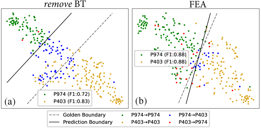
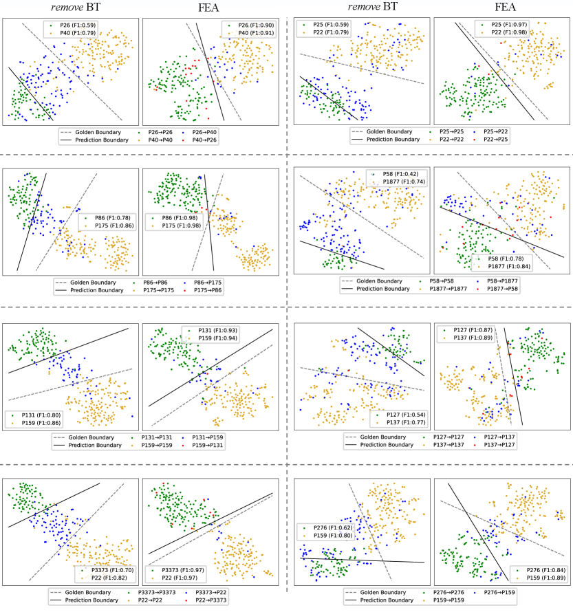
Compared with “remove BT”, Fea reduces a lot of latter errors, and thus alleviates the catastrophic forgetting. To explain why BT can reduce the latter error, we chose two similar relations P974 (tributary, appears at the -th task) and P403 (mouth of the watercourse, appears at the -th task) with severe latter error to conduct a case study.555Please refer to Appendix F for more cases. We draw the t-SNE of instances belonging to P974 and P403 for “remove BT” and Fea after learning P403. As shown in Figure 1(a), for “remove BT”, the model tends to establish a skewed decision boundary between P974 and P403 due to the data imbalance.666The skewed boundary phenomenon between minor and majority classes is also observed in imbalanced learning works Khan et al. (2019); Kim and Kim (2020). In contrast, Fea with BT can establish a more balanced decision boundary (Figure1(b)), and thus reduces a lot of latter error. To further confirm whether BT helps build a better decision boundary, we drop the classifier of Fea and “remove BT” after training, and retrain an upper-bound classifier (UBC) with all training data to see their performance gap. As shown in the first four rows of Table 4: 1) Fea outperforms “remove BT”, while “Fea with UBC” and “remove BT with UBC” have comparable results on two benchmarks, showing that BT works because it establishes a more balanced decision boundary. 2) Fea significantly outperforms “remove BT” average accuracy on two benchmarks, showing that the intrinsic data imbalance problem between old and new data that leads to a skewed decision boundary is one of the main reasons for catastrophic forgetting.
We also explore the performance of supervised method that trains all data together without catastrophic forgetting. As shown in Table 4: 1) two CRE models “with UBC” and “SUP.” significantly outperform “SUP. with frozen encoder”, which shows the original BERT representation is not good enough to represent relations, and the pretrained encoder learns a lot of knowledge during training. 2) “SUP.” significantly outperforms Fea and “remove BT” and average accuracy on two benchmarks, while it just outperforms “Fea with UBC” and “remove BT with UBC” and average accuracy, showing that the forgetting of BERT encoder may be not a serious problem for the performance of CRE models. 3) “with UBC” significantly improves the performances of Fea and “remove BT” and average accuracy on two benchmarks, showing that constructing a good classifier can be of great benefit to CRE models.
| Methods | Few. | Tac. | Avg. |
|---|---|---|---|
| Fea | 84.3 | 77.7 | 81.0 |
| Fea with UBC | 88.0 | 82.0 | 85.0 |
| remove BT | 75.8 | 71.2 | 73.5 |
| remove BT with UBC | 87.9 | 82.4 | 85.2 |
| Supervised (SUP.) | 89.5 | 84.5 | 87.0 |
| SUP. with frozen encoder | 77.3 | 66.2 | 71.8 |
6.4 Explorations of Fast Adaption
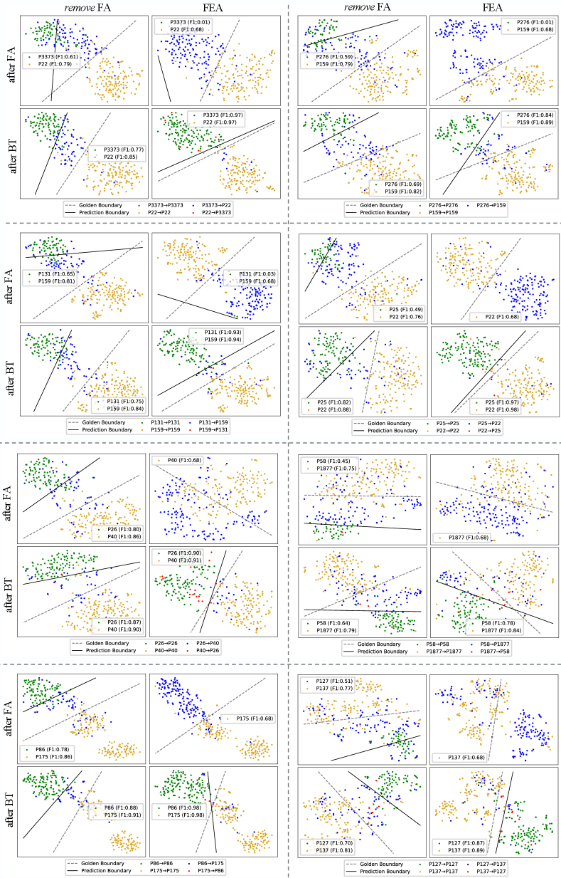
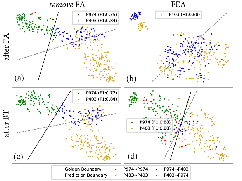
Fea outperforms “remove FA” average accuracy on two benchmarks, showing the importance of training the model ONLY on new data at first. Table 3 shows FA works since it is helpful for reducing the latter error. Therefore, we begin with a case study between P974 and P403 with severe latter error to understand why FA is helpful.777Please refer to Appendix G for more cases. We draw the t-SNE of instances belonging to P974 and P403 for “remove FA” and Fea after two learning stages of the task containing P403. For “remove FA”, after the first stage, the model establishes a skewed decision boundary due to the data imbalance problem (Figure 2(a)). However, after BT, the decision boundary is still skewed (Figure 2(c)), showing BT does not work well. For Fea, in contrast, after FA, the memory instances of P974 and P403 scatter on the embedding space, and the model predicts all instances as P403 (Figure 2(b)), because the model does not need to distinguish these two relations. After BT, the model establishes a relative fair decision boundary (Figure 2(d)) compared with that of “remove FA”. These results show that “remove FA” may hinder the following BT.
Because BT updates the model on the memory data, we further utilize the gradient norm of memory data to reflect their effect on BT. As shown in Table 5, in the BT stage, compared with Fea, the memory data has a much smaller gradient norm in “remove FA”, which shows the memory data has a very limited effect. We think the reasons are as follows: 1) For “remove FA”, the model has learned a good parameter to distinguish the memory data between old and new relations at the first stage, and thus tends to keep the learned parameter (i.e., skewed decision boundary) in the following BT. 2) In contrast, Fea utilizes the memory data only in BT, and thus can help the model establish a more balanced decision boundary on the balanced situation from the scratch. These results show that it is important to learn new relations with only new data at first, and FA works as it retains the potential of memory data for the subsequent BT.
6.5 Less is More: Rethinking CRE models
In this section, we find that Fea can be viewed as a simplified variant of two strong CRE models (EMAR and RPCRE), and we rethink them to explain why Fea can outperform these more complex models. We hope our analysis can provide guidance for the design of future CRE models.
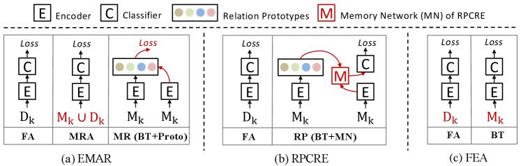
Rethinking EMAR
Han et al. (2020) proposes an episodic memory activation and reconsolidation (EMAR) method for CRE. As shown in Figure 3(a), EMAR consists of three stages: 1) Learning from new data. 2) Memory Replay and Activation (MRA): Learning from the memory data and new data. 3) Memory Reconsolidation (MR): learning from memory data with relation prototypes. Please refer to Han et al. (2020) for more model details.
Among these three stages, the first stage is the same as FA, and the third stage MR can be regarded as BT (compared with BT, MR further incorporates relation prototypes to train the model). However, the extra second stage MAR mixes the memory and new data to train the model, and thus introduces the data imbalance problem. According to our analysis, the data imbalance harms the model performance. Therefore, we only use the balanced memory data to train the model in MRA. As shown in Table 6, after using balanced data in MRA (EMAR: balanced MRA), the accuracy of EMAR on Fewrel and Tacred can improve and , respectively. However, the performance is still slightly lower than that of Fea, which shows incorporating the relation prototypes may not be helpful in CRE. As the relation prototypes are calculated by the memory data, we think the reason is that optimizing the model based on relation prototypes aggravates the over-fitting of memory data.
| Methods | Fewrel | Tacred |
|---|---|---|
| Fea | 27.8 | 45.0 |
| remove FA | 1.4 | 4.1 |
| Methods | Fewrel | Tacred |
|---|---|---|
| Fea | 84.3 | 77.7 |
| EMAR | 83.6 | 76.1 |
| EMAR: balanced MRA | 84.0 | 77.2 |
| RPCRE | 82.8 | 75.3 |
| RPCRE: with normalized | 83.0 | 76.5 |
Rethinking RPCRE
Cui et al. (2021) proposes a refining network with relation prototypes for CRE (RPCRE). As shown in Figure 3(b), RPCRE consists of two learning stages: 1) Initial training for new task. 2) Refine input instance with Prototypes (RP): Train a memory network (MN) to refine the representation of input instances with the relation prototypes for better classification. Please refer to Cui et al. (2021) for more model details.
The first stage is FA, and the second stage RP can be regarded as BT. Compared with BT, RP further utilizes a memory network (MN) to refine the representation of the input instances with relation prototypes. Specifically, for each input instance, MN regards it as a query, the relation prototypes as key and value. MN uses an attention mechanism to aggregate the relation prototypes, and adds the aggregation result to the original representation as a refined representation for classification.
However, MN is harmful for performance. There exists two potential reasons: 1) MN incorporates implicit data imbalance. We find that there exists gaps among the norms of different prototypes and input instances tend to attention more to the relation prototype with the larger norm. Therefore, after refining, the representation of each relation is not balanced. To alleviate this problem, we normalize the norm of all relation prototypes to (“with normalized”). As shown in Table 6, after normalizing, the accuracy of RPCRE on Fewrel and Tacred can improve and , respectively. 2) MN makes it more difficult for the CRE model to distinguish similar relations. According to our error analysis in Section 6.2, CRE models are confused by the similar relations, and are prone to latter error. Given an instance, the attention-based MN mechanism tends to add the representation of its similar relation prototypes to it, and thus the representation of similar relations becomes more confusing. For example, RPCRE predicts instances of former relation “followed by” to latter relation “follow”, and vice versa, while the ratio of pure Fea is much less than that of RPCRE ( and , respectively).
6.6 Suggestions for Future Work
Through our a series of analysis on both Fea and two strong CRE baselines, we think future CRE models should pay attention to the following issues: 1) Learn distinguishable feature for similar relations. In CRE, the catastrophic forgetting mainly happens among similar relations from different tasks, since there does not exist enough data to teach the model to distinguish them. Therefore, it may be helpful to propose some mechanisms to learn distinguishable features that highlight differences among similar relations. 2) Establish a better classifier. In CRE, the forgetting that happens on the pretrained encoder is not serious, and the conventional Softmax classifier tends to build a skewed decision boundary, leading to severe latter errors. Therefore, it can be helpful to design a better classifier for CRE models.
7 Conclusion
In this paper, we propose a frustratingly easy but effective approach (Fea) for CRE. Fea consists of two stages: 1) Fast Adaption (FA) warms up the model with only new data. 2) Balanced Tuning (BT) circumvents the intrinsic imbalance between new and old relations by finetuning on the balanced memory data. Despite the simplicity of Fea, it is extremely effective. Therefore, we conduct a series of analysis to understand why Fea works and why catastrophic forgetting happens. We also dive into two strong CRE baselines, and find that Fea can be viewed as a simplified but most effective variant of them. We show these two CRE baselines can be further enhanced by the principle of Fea. Based on our analysis, we also provide two actionable suggestions for future model design in CRE.
References
- Aljundi et al. (2018) Rahaf Aljundi, Francesca Babiloni, Mohamed Elhoseiny, Marcus Rohrbach, and Tinne Tuytelaars. 2018. Memory aware synapses: Learning what (not) to forget. In Proceedings of the European Conference on Computer Vision (ECCV), pages 139–154.
- Alt et al. (2019) Christoph Alt, Marc Hübner, and Leonhard Hennig. 2019. Improving relation extraction by pre-trained language representations. arXiv preprint arXiv:1906.03088.
- Baldini Soares et al. (2019) Livio Baldini Soares, Nicholas FitzGerald, Jeffrey Ling, and Tom Kwiatkowski. 2019. Matching the blanks: Distributional similarity for relation learning. In Proceedings of the 57th Annual Meeting of the Association for Computational Linguistics, pages 2895–2905, Florence, Italy. Association for Computational Linguistics.
- Biesialska et al. (2020) Magdalena Biesialska, Katarzyna Biesialska, and Marta R. Costa-jussà. 2020. Continual lifelong learning in natural language processing: A survey. In Proceedings of the 28th International Conference on Computational Linguistics, pages 6523–6541, Barcelona, Spain (Online). International Committee on Computational Linguistics.
- Cui et al. (2021) Li Cui, Deqing Yang, Jiaxin Yu, Chengwei Hu, Jiayang Cheng, Jingjie Yi, and Yanghua Xiao. 2021. Refining sample embeddings with relation prototypes to enhance continual relation extraction. In Proceedings of the 59th Annual Meeting of the Association for Computational Linguistics and the 11th International Joint Conference on Natural Language Processing (Volume 1: Long Papers), pages 232–243, Online. Association for Computational Linguistics.
- Gormley et al. (2015) Matthew R. Gormley, Mo Yu, and Mark Dredze. 2015. Improved relation extraction with feature-rich compositional embedding models. In Proceedings of the 2015 Conference on Empirical Methods in Natural Language Processing, pages 1774–1784, Lisbon, Portugal. Association for Computational Linguistics.
- Han et al. (2020) Xu Han, Yi Dai, Tianyu Gao, Yankai Lin, Zhiyuan Liu, Peng Li, Maosong Sun, and Jie Zhou. 2020. Continual relation learning via episodic memory activation and reconsolidation. In Proceedings of the 58th Annual Meeting of the Association for Computational Linguistics, pages 6429–6440, Online. Association for Computational Linguistics.
- Han et al. (2018a) Xu Han, Pengfei Yu, Zhiyuan Liu, Maosong Sun, and Peng Li. 2018a. Hierarchical relation extraction with coarse-to-fine grained attention. In Proceedings of the 2018 Conference on Empirical Methods in Natural Language Processing, pages 2236–2245, Brussels, Belgium. Association for Computational Linguistics.
- Han et al. (2018b) Xu Han, Hao Zhu, Pengfei Yu, Ziyun Wang, Yuan Yao, Zhiyuan Liu, and Maosong Sun. 2018b. FewRel: A large-scale supervised few-shot relation classification dataset with state-of-the-art evaluation. In Proceedings of the 2018 Conference on Empirical Methods in Natural Language Processing, pages 4803–4809, Brussels, Belgium. Association for Computational Linguistics.
- Khan et al. (2019) Salman Khan, Munawar Hayat, Syed Waqas Zamir, Jianbing Shen, and Ling Shao. 2019. Striking the right balance with uncertainty. In 2019 IEEE/CVF Conference on Computer Vision and Pattern Recognition (CVPR), pages 103–112.
- Kim and Kim (2020) Byungju Kim and Junmo Kim. 2020. Adjusting decision boundary for class imbalanced learning. IEEE Access, 8:81674–81685.
- Kirkpatrick et al. (2017) James Kirkpatrick, Razvan Pascanu, Neil Rabinowitz, Joel Veness, Guillaume Desjardins, Andrei A Rusu, Kieran Milan, John Quan, Tiago Ramalho, Agnieszka Grabska-Barwinska, et al. 2017. Overcoming catastrophic forgetting in neural networks. Proceedings of the national academy of sciences, 114(13):3521–3526.
- Li and Hoiem (2017) Zhizhong Li and Derek Hoiem. 2017. Learning without forgetting. IEEE transactions on pattern analysis and machine intelligence, 40(12):2935–2947.
- Lin et al. (2016) Yankai Lin, Shiqi Shen, Zhiyuan Liu, Huanbo Luan, and Maosong Sun. 2016. Neural relation extraction with selective attention over instances. In Proceedings of the 54th Annual Meeting of the Association for Computational Linguistics (Volume 1: Long Papers), pages 2124–2133, Berlin, Germany. Association for Computational Linguistics.
- Liu et al. (2018) Chenxi Liu, Barret Zoph, Maxim Neumann, Jonathon Shlens, Wei Hua, Li-Jia Li, Li Fei-Fei, Alan Yuille, Jonathan Huang, and Kevin Murphy. 2018. Progressive neural architecture search. In Proceedings of the European conference on computer vision (ECCV), pages 19–34.
- Liu et al. (2019) Hongtao Liu, Peiyi Wang, Fangzhao Wu, Pengfei Jiao, Wenjun Wang, Xing Xie, and Yueheng Sun. 2019. Reet: Joint relation extraction and entity typing via multi-task learning. In CCF International Conference on Natural Language Processing and Chinese Computing, pages 327–339. Springer.
- Lopez-Paz and Ranzato (2017) David Lopez-Paz and Marc’Aurelio Ranzato. 2017. Gradient episodic memory for continual learning. Advances in neural information processing systems, 30:6467–6476.
- Mallya et al. (2018) Arun Mallya, Dillon Davis, and Svetlana Lazebnik. 2018. Piggyback: Adapting a single network to multiple tasks by learning to mask weights. In Proceedings of the European Conference on Computer Vision (ECCV), pages 67–82.
- Mallya and Lazebnik (2018) Arun Mallya and Svetlana Lazebnik. 2018. Packnet: Adding multiple tasks to a single network by iterative pruning. In Proceedings of the IEEE conference on Computer Vision and Pattern Recognition, pages 7765–7773.
- Mintz et al. (2009) Mike Mintz, Steven Bills, Rion Snow, and Daniel Jurafsky. 2009. Distant supervision for relation extraction without labeled data. In Proceedings of the Joint Conference of the 47th Annual Meeting of the ACL and the 4th International Joint Conference on Natural Language Processing of the AFNLP, pages 1003–1011, Suntec, Singapore. Association for Computational Linguistics.
- Miwa and Bansal (2016) Makoto Miwa and Mohit Bansal. 2016. End-to-end relation extraction using LSTMs on sequences and tree structures. In Proceedings of the 54th Annual Meeting of the Association for Computational Linguistics (Volume 1: Long Papers), pages 1105–1116, Berlin, Germany. Association for Computational Linguistics.
- Riedel et al. (2013) Sebastian Riedel, Limin Yao, Andrew McCallum, and Benjamin M. Marlin. 2013. Relation extraction with matrix factorization and universal schemas. In Proceedings of the 2013 Conference of the North American Chapter of the Association for Computational Linguistics: Human Language Technologies, pages 74–84, Atlanta, Georgia. Association for Computational Linguistics.
- Seff et al. (2017) Ari Seff, Alex Beatson, Daniel Suo, and Han Liu. 2017. Continual learning in generative adversarial nets. arXiv preprint arXiv:1705.08395.
- Serra et al. (2018) Joan Serra, Didac Suris, Marius Miron, and Alexandros Karatzoglou. 2018. Overcoming catastrophic forgetting with hard attention to the task. In International Conference on Machine Learning, pages 4548–4557. PMLR.
- Shin et al. (2017) Hanul Shin, Jung Kwon Lee, Jaehong Kim, and Jiwon Kim. 2017. Continual learning with deep generative replay. In Proceedings of the 31st International Conference on Neural Information Processing Systems, pages 2994–3003.
- Wang et al. (2019) Hong Wang, Wenhan Xiong, Mo Yu, Xiaoxiao Guo, Shiyu Chang, and William Yang Wang. 2019. Sentence embedding alignment for lifelong relation extraction. In Proceedings of the 2019 Conference of the North American Chapter of the Association for Computational Linguistics: Human Language Technologies, Volume 1 (Long and Short Papers), pages 796–806, Minneapolis, Minnesota. Association for Computational Linguistics.
- Wu et al. (2021) Tongtong Wu, Xuekai Li, Yuan-Fang Li, Gholamreza Haffari, Guilin Qi, Yujin Zhu, and Guoqiang Xu. 2021. Curriculum-meta learning for order-robust continual relation extraction. In Proceedings of the AAAI Conference on Artificial Intelligence, volume 35, pages 10363–10369.
- Xu et al. (2015a) Yan Xu, Lili Mou, Ge Li, Yunchuan Chen, Hao Peng, and Zhi Jin. 2015a. Classifying relations via long short term memory networks along shortest dependency paths. In Proceedings of the 2015 Conference on Empirical Methods in Natural Language Processing, pages 1785–1794, Lisbon, Portugal. Association for Computational Linguistics.
- Xu et al. (2015b) Yan Xu, Lili Mou, Ge Li, Yunchuan Chen, Hao Peng, and Zhi Jin. 2015b. Classifying relations via long short term memory networks along shortest dependency paths. In Proceedings of the 2015 Conference on Empirical Methods in Natural Language Processing, pages 1785–1794, Lisbon, Portugal. Association for Computational Linguistics.
- Zelenko et al. (2003) Dmitry Zelenko, Chinatsu Aone, and Anthony Richardella. 2003. Kernel methods for relation extraction. Journal of machine learning research, 3(Feb):1083–1106.
- Zeng et al. (2015) Daojian Zeng, Kang Liu, Yubo Chen, and Jun Zhao. 2015. Distant supervision for relation extraction via piecewise convolutional neural networks. In Proceedings of the 2015 Conference on Empirical Methods in Natural Language Processing, pages 1753–1762, Lisbon, Portugal. Association for Computational Linguistics.
- Zeng et al. (2014) Daojian Zeng, Kang Liu, Siwei Lai, Guangyou Zhou, and Jun Zhao. 2014. Relation classification via convolutional deep neural network. In Proceedings of COLING 2014, the 25th International Conference on Computational Linguistics: Technical Papers, pages 2335–2344, Dublin, Ireland. Dublin City University and Association for Computational Linguistics.
- Zhang et al. (2018) Yuhao Zhang, Peng Qi, and Christopher D. Manning. 2018. Graph convolution over pruned dependency trees improves relation extraction. In Proceedings of the 2018 Conference on Empirical Methods in Natural Language Processing, pages 2205–2215, Brussels, Belgium. Association for Computational Linguistics.
- Zhang et al. (2017) Yuhao Zhang, Victor Zhong, Danqi Chen, Gabor Angeli, and Christopher D. Manning. 2017. Position-aware attention and supervised data improve slot filling. In Proceedings of the 2017 Conference on Empirical Methods in Natural Language Processing, pages 35–45, Copenhagen, Denmark. Association for Computational Linguistics.
- Zhao et al. (2022) Kang Zhao, Hua Xu, Jiangong Yang, and Kai Gao. 2022. Consistent representation learning for continual relation extraction. arXiv preprint arXiv:2203.02721.
- Zhou et al. (2005) GuoDong Zhou, Jian Su, Jie Zhang, and Min Zhang. 2005. Exploring various knowledge in relation extraction. In Proceedings of the 43rd Annual Meeting of the Association for Computational Linguistics (ACL’05), pages 427–434, Ann Arbor, Michigan. Association for Computational Linguistics.
Appendix A Baselines
We compared Fea with following baselines:
-
•
EA-EMR Wang et al. (2019), which uses an embedding alignment mechanism to maintain memory to alleviate the catastrophic forgetting problem.
-
•
CML Wu et al. (2021), which proposes a curriculum-meta learning method to alleviate catastrophic forgetting while maintaining order-robust.
-
•
EMAR Han et al. (2020), which introduces memory activation and reconsolidation mechanism for continual relation extraction.
-
•
RP-CRE Cui et al. (2021), which refines sample embeddings with relation prototypes to enhance continual relation extraction.
-
•
CRL Zhao et al. (2022), which proposes a consistent representation learning method that utilizes contrastive replay and knowledge distillation to alleviate catastrophic forgetting.
| Ablation Methods | Stage 1 | Stage 2 | Fewrel | Tacred |
|---|---|---|---|---|
| Fea | 84.3 | 77.7 | ||
| A1 (remove BT) | 75.8 | 71.2 | ||
| A2 (remove FA) | 81.1 | 74.9 | ||
| A3 (remove FA and BT) | 75.6 | 71.2 | ||
| A4 | 73.1 | 70.1 | ||
| A5 | 78.1 | 73.8 |
Appendix B Influence of Memory Size
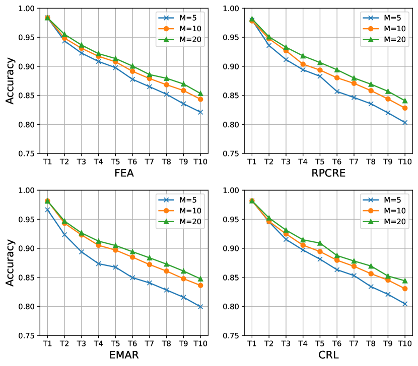
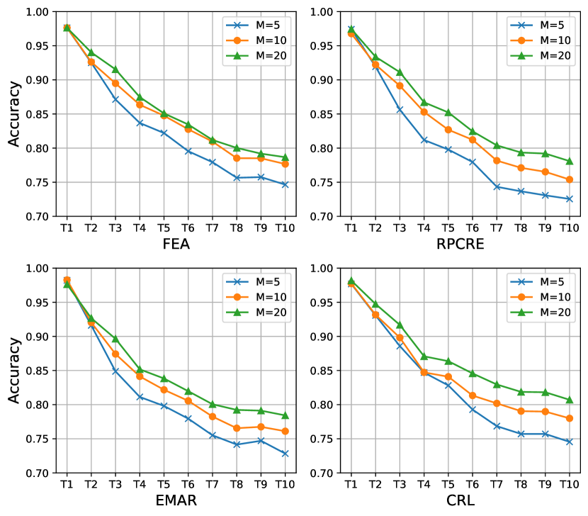
For the rehearsal-based CRE models, memory size (the number of stored instances for each relation) is a key factor for the model performance. Therefore, in this section, we also study the performance of Fea with different memory sizes. As shown in Figure 4 and Figure 5: 1) As the size of the memory decreases, the performances of all models drop, which shows the importance of the memory size for CRE models. 2) In Fewrel, Fea outperforms three baselines with different memory sizes. In addition, when decreasing the memory size, the performance gap between Fea and baselines tends to be larger. For example, on the final task, Fea outperforms RPCRE , and accuracy on memory size , and , respectively. 3) In Tacred, Fea outperforms RPCRE and EMAR with three different memory sizes, especially when memory sizes are and . CRL outperforms Fea when memory size is . However, when memory size is and , Fea achieves comparable results with CRL. These results show Fea has more obvious advantages when the memory size is small. (4) By comparing the performance gap of between and , we can also find Fea performs more stable than all baselines.
Appendix C Model Efficiency
| Models | Fewrel | Tacred | ||
|---|---|---|---|---|
| Accuracy | Time | Accuracy | Time | |
| Fea | 84.3 | 173.7s | 77.7 | 53.8s |
| RPCRE | 82.8 | 347.2s | 75.3 | 89.8s |
| EMAR | 83.6 | 297.3s | 76.1 | 70.8s |
| CRL | 83.1 | 256.2s | 78.0 | 67.7s |
In real life, CRE models need to learn new relations constantly, thus we should also consider the learning efficiency of models. In this section, we compared the learning time (average training time per task) of Fea and our baselines on two benchmarks. As shown in Table 8, with exactly the same hardware setting, compared with all strong baselines, Fea has a better learning efficiency.
Appendix D More Detail of Ablation Study
In Table 7, We explore different kinds of ablation methods in total. denotes the up-sampling memory data where the number of memory data for each previously learned relation is the same as that of its origin training data. As is shown: 1) A3 and A4 have poor performances on two benchmarks, showing that it is important to propose a two-stage learning CRE model. 2) A5 outperforms A4, showing that it is important to learn new relations at stage 1. Fea outperform A2 shows that stage 1 should have ONLY new data. 3) Fea and A2 outperform all other methods showing that it is important to ensure the data imbalance at stage 2.
Appendix E More Detail of Error Analysis
To better explore the effectiveness of BT and FA, we conduct error analysis for Fea, “BT: remove BT” and “remove FA” on Fewrel in in Table 9 and Table 10. From the results, we can find: 1) The model makes a lot of latter error. 2) The model wrongly predicts many instances as the relations appearing at the last task (i.e., [10]). 3) The model is unable to distinguish similarity relations, and easily predicts former-occurring relation instances as the later-occurring similar relation. For example, “followed by (P156, appear at task [1])” to “follow (P155, appears at task [8])”, “mother” (P25, appears at task [4]) to “father” (P22, appears at task [10]), “tributary (P974, appears at task [7])” to “mouth of the watercourse (P403, appears at task [9])”. (4) Removing either BT or FA will significantly increase the latter error, and thus aggravate the catastrophic forgetting.
Appendix F Effectiveness of BT
We draw several relation pairs with severe latter error to show the effectiveness of BT in Figure 6.
Appendix G Effectiveness of FA
We draw several relation pairs with severe latter error to show the effectiveness of FA in Figure 7.
| Relations | Fea | remove BT | remove FA | ||||||
|---|---|---|---|---|---|---|---|---|---|
| Acc. | TOP1 | TOP2 | Acc. | TOP1 | TOP2 | Acc. | TOP1 | TOP2 | |
| P156/[1] | 0.52 | P155/[8]/0.31 | P176/[10]/0.02 | 0.36 | P155/[8]/0.31 | P31/[10]/0.15 | 0.43 | P155/[8]/0.27 | P31/[10]/0.09 |
| P84/[1] | 0.94 | P127/[5]/0.03 | P6/[3]/0.01 | 0.91 | P176/[10]/0.04 | P127/[5]/0.02 | 0.93 | P31/[10]/0.01 | P1877/[10]/0.01 |
| P39/[1] | 0.94 | P106/[4]/0.02 | P410/[1]/0.01 | 0.88 | P31/[10]/0.04 | P106/[4]/0.04 | 0.92 | P106/[4]/0.04 | P31/[10]/0.01 |
| P276/[1] | 0.52 | P159/[10]/0.21 | P551/[7]/0.04 | 0.34 | P159/[10]/0.52 | P31/[10]/0.04 | 0.46 | P159/[10]/0.37 | P706/[5]/0.04 |
| P410/[1] | 0.99 | P39/[1]/0.01 | P106/[4]/0.01 | 0.98 | P241/[1]/0.01 | P31/[10]/0.01 | 0.99 | P106/[4]/0.01 | P26/[8]/0.00 |
| P241/[1] | 0.91 | P137/[7]/0.05 | P27/[8]/0.01 | 0.88 | P137/[7]/0.04 | P407/[10]/0.04 | 0.81 | P137/[7]/0.11 | P27/[8]/0.03 |
| P177/[1] | 1.00 | P137/[7]/0.00 | P937/[7]/0.00 | 0.98 | P4552/[6]/0.01 | P206/[6]/0.01 | 0.99 | P206/[6]/0.01 | P3450/[7]/0.00 |
| P264/[1] | 0.95 | P175/[9]/0.03 | P463/[5]/0.01 | 0.92 | P175/[9]/0.02 | P176/[10]/0.01 | 0.90 | P175/[9]/0.04 | P750/[4]/0.03 |
| P412/[2] | 0.99 | P1303/[8]/0.01 | P178/[7]/0.00 | 0.97 | P1303/[8]/0.03 | P178/[7]/0.00 | 0.99 | P1303/[8]/0.01 | P178/[7]/0.00 |
| P361/[2] | 0.27 | P31/[10]/0.11 | P131/[2]/0.07 | 0.21 | P31/[10]/0.31 | P1344/[10]/0.08 | 0.22 | P31/[10]/0.21 | P527/[8]/0.06 |
| P1923/[2] | 0.95 | P1346/[4]/0.03 | P710/[2]/0.01 | 0.87 | P1346/[4]/0.07 | P159/[10]/0.01 | 0.88 | P1346/[4]/0.07 | P710/[2]/0.04 |
| P123/[2] | 0.59 | P178/[7]/0.34 | P750/[4]/0.02 | 0.45 | P178/[7]/0.37 | P176/[10]/0.06 | 0.52 | P178/[7]/0.34 | P176/[10]/0.07 |
| P118/[2] | 0.96 | P641/[10]/0.02 | P1344/[10]/0.01 | 0.88 | P1344/[10]/0.06 | P641/[10]/0.04 | 0.93 | P1344/[10]/0.04 | P641/[10]/0.03 |
| P131/[2] | 0.66 | P159/[10]/0.09 | P706/[5]/0.09 | 0.44 | P159/[10]/0.31 | P31/[10]/0.08 | 0.46 | P159/[10]/0.21 | P17/[6]/0.06 |
| P710/[2] | 0.72 | P1346/[4]/0.06 | P1923/[2]/0.06 | 0.66 | P1346/[4]/0.08 | P1877/[10]/0.06 | 0.79 | P1346/[4]/0.05 | P991/[4]/0.04 |
| P355/[2] | 0.69 | P527/[8]/0.11 | P127/[5]/0.03 | 0.56 | P31/[10]/0.18 | P159/[10]/0.15 | 0.60 | P159/[10]/0.10 | P127/[5]/0.07 |
| P6/[3] | 0.99 | P991/[4]/0.01 | P355/[2]/0.01 | 0.98 | P991/[4]/0.01 | P22/[10]/0.01 | 0.99 | P1877/[10]/0.01 | P991/[4]/0.01 |
| P400/[3] | 0.91 | P306/[9]/0.09 | P31/[10]/0.01 | 0.84 | P306/[9]/0.11 | P31/[10]/0.04 | 0.82 | P306/[9]/0.16 | P361/[2]/0.01 |
| P101/[3] | 0.79 | P135/[6]/0.04 | P31/[10]/0.03 | 0.61 | P31/[10]/0.15 | P106/[4]/0.07 | 0.68 | P106/[4]/0.10 | P31/[10]/0.06 |
| P140/[3] | 0.95 | P407/[10]/0.01 | P101/[3]/0.01 | 0.88 | P31/[10]/0.06 | P407/[10]/0.03 | 0.93 | P407/[10]/0.02 | P31/[10]/0.01 |
| P2094/[3] | 1.00 | P137/[7]/0.00 | P937/[7]/0.00 | 0.99 | P1344/[10]/0.01 | P937/[7]/0.00 | 0.99 | P1344/[10]/0.01 | P937/[7]/0.00 |
| P364/[3] | 0.86 | P407/[10]/0.13 | P27/[8]/0.01 | 0.67 | P407/[10]/0.33 | P3450/[7]/0.00 | 0.68 | P407/[10]/0.31 | P495/[4]/0.01 |
| P150/[3] | 0.94 | P1001/[6]/0.02 | P551/[7]/0.01 | 0.89 | P159/[10]/0.08 | P31/[10]/0.01 | 0.86 | P159/[10]/0.09 | P527/[8]/0.01 |
| P466/[3] | 0.92 | P127/[5]/0.03 | P140/[3]/0.01 | 0.76 | P159/[10]/0.09 | P137/[7]/0.04 | 0.88 | P159/[10]/0.04 | P127/[5]/0.03 |
| P449/[4] | 0.98 | P750/[4]/0.01 | P1408/[5]/0.01 | 0.97 | P750/[4]/0.02 | P31/[10]/0.01 | 0.94 | P750/[4]/0.04 | P137/[7]/0.02 |
| P674/[4] | 0.81 | P1877/[10]/0.06 | P527/[8]/0.04 | 0.69 | P1877/[10]/0.25 | P527/[8]/0.03 | 0.78 | P1877/[10]/0.14 | P527/[8]/0.02 |
| P991/[4] | 0.97 | P6/[3]/0.02 | P102/[9]/0.01 | 0.99 | P102/[9]/0.01 | P137/[7]/0.00 | 0.98 | P6/[3]/0.01 | P102/[9]/0.01 |
| P495/[4] | 0.72 | P407/[10]/0.11 | P27/[8]/0.06 | 0.31 | P407/[10]/0.46 | P27/[8]/0.08 | 0.56 | P407/[10]/0.17 | P27/[8]/0.09 |
| P1346/[4] | 0.79 | P1923/[2]/0.14 | P710/[2]/0.05 | 0.83 | P1923/[2]/0.09 | P1877/[10]/0.04 | 0.82 | P1923/[2]/0.11 | P710/[2]/0.04 |
| P750/[4] | 0.89 | P449/[4]/0.03 | P178/[7]/0.02 | 0.89 | P178/[7]/0.04 | P176/[10]/0.04 | 0.91 | P176/[10]/0.02 | P178/[7]/0.01 |
| P106/[4] | 0.69 | P641/[10]/0.13 | P101/[3]/0.11 | 0.69 | P641/[10]/0.13 | P1303/[8]/0.07 | 0.79 | P641/[10]/0.11 | P1303/[8]/0.06 |
| P25/[4] | 0.91 | P22/[10]/0.05 | P26/[8]/0.02 | 0.39 | P22/[10]/0.59 | P26/[8]/0.03 | 0.69 | P22/[10]/0.30 | P26/[8]/0.01 |
| P706/[5] | 0.67 | P206/[6]/0.12 | P4552/[6]/0.09 | 0.59 | P206/[6]/0.11 | P31/[10]/0.11 | 0.54 | P206/[6]/0.13 | P4552/[6]/0.10 |
| P127/[5] | 0.51 | P137/[7]/0.17 | P176/[10]/0.09 | 0.29 | P176/[10]/0.30 | P137/[7]/0.19 | 0.36 | P137/[7]/0.21 | P176/[10]/0.20 |
| P413/[5] | 1.00 | P137/[7]/0.00 | P937/[7]/0.00 | 1.00 | P137/[7]/0.00 | P937/[7]/0.00 | 1.00 | P137/[7]/0.00 | P937/[7]/0.00 |
| P463/[5] | 0.81 | P102/[9]/0.01 | P175/[9]/0.01 | 0.64 | P31/[10]/0.16 | P175/[9]/0.05 | 0.70 | P31/[10]/0.09 | P175/[9]/0.04 |
| P1408/[5] | 0.99 | P740/[5]/0.01 | P3450/[7]/0.00 | 0.91 | P159/[10]/0.09 | P407/[10]/0.01 | 0.98 | P159/[10]/0.01 | P17/[6]/0.01 |
| P59/[5] | 0.99 | P22/[10]/0.01 | P137/[7]/0.00 | 0.95 | P31/[10]/0.04 | P22/[10]/0.01 | 0.99 | P460/[9]/0.01 | P31/[10]/0.01 |
| P86/[5] | 0.74 | P58/[8]/0.10 | P175/[9]/0.06 | 0.29 | P1877/[10]/0.51 | P175/[9]/0.15 | 0.70 | P175/[9]/0.14 | P1877/[10]/0.12 |
| P740/[5] | 0.77 | P159/[10]/0.18 | P937/[7]/0.02 | 0.67 | P159/[10]/0.32 | P27/[8]/0.01 | 0.66 | P159/[10]/0.29 | P937/[7]/0.01 |
| Relations | Fea | BT: remove BT | remove FA | ||||||
|---|---|---|---|---|---|---|---|---|---|
| Acc. | TOP1 | TOP2 | Acc. | TOP1 | TOP2 | Acc. | TOP1 | TOP2 | |
| P206/[6] | 0.90 | P706/[5]/0.03 | P403/[9]/0.03 | 0.89 | P150/[3]/0.04 | P403/[9]/0.03 | 0.93 | P403/[9]/0.04 | P706/[5]/0.01 |
| P17/[6] | 0.71 | P495/[4]/0.09 | P407/[10]/0.07 | 0.64 | P407/[10]/0.16 | P159/[10]/0.08 | 0.72 | P407/[10]/0.09 | P1001/[6]/0.07 |
| P136/[6] | 0.87 | P31/[10]/0.05 | P641/[10]/0.02 | 0.76 | P31/[10]/0.15 | P641/[10]/0.03 | 0.82 | P31/[10]/0.09 | P641/[10]/0.03 |
| P800/[6] | 0.94 | P176/[10]/0.01 | P551/[7]/0.01 | 0.89 | P31/[10]/0.06 | P176/[10]/0.01 | 0.93 | P86/[5]/0.01 | P31/[10]/0.01 |
| P4552/[6] | 0.91 | P706/[5]/0.06 | P31/[10]/0.01 | 0.91 | P31/[10]/0.06 | P706/[5]/0.02 | 0.96 | P706/[5]/0.02 | P31/[10]/0.01 |
| P1001/[6] | 0.81 | P495/[4]/0.06 | P17/[6]/0.04 | 0.64 | P159/[10]/0.16 | P31/[10]/0.09 | 0.84 | P159/[10]/0.07 | P31/[10]/0.03 |
| P931/[6] | 0.96 | P159/[10]/0.03 | P706/[5]/0.01 | 0.94 | P159/[10]/0.06 | P137/[7]/0.01 | 0.94 | P159/[10]/0.06 | P137/[7]/0.00 |
| P135/[6] | 0.88 | P463/[5]/0.03 | P937/[7]/0.01 | 0.85 | P31/[10]/0.06 | P1344/[10]/0.01 | 0.88 | P31/[10]/0.02 | P101/[3]/0.02 |
| P3373/[7] | 0.68 | P22/[10]/0.16 | P40/[9]/0.11 | 0.54 | P22/[10]/0.38 | P40/[9]/0.04 | 0.77 | P22/[10]/0.09 | P40/[9]/0.09 |
| P551/[7] | 0.69 | P937/[7]/0.20 | P27/[8]/0.04 | 0.56 | P159/[10]/0.18 | P937/[7]/0.14 | 0.63 | P937/[7]/0.21 | P159/[10]/0.07 |
| P974/[7] | 0.90 | P403/[9]/0.10 | P3450/[7]/0.00 | 0.60 | P403/[9]/0.39 | P131/[2]/0.01 | 0.54 | P403/[9]/0.45 | P155/[8]/0.01 |
| P921/[7] | 0.75 | P31/[10]/0.05 | P641/[10]/0.04 | 0.51 | P31/[10]/0.29 | P1877/[10]/0.06 | 0.67 | P31/[10]/0.13 | P1877/[10]/0.04 |
| P3450/[7] | 0.99 | P641/[10]/0.01 | P937/[7]/0.00 | 0.93 | P31/[10]/0.04 | P1344/[10]/0.01 | 0.93 | P31/[10]/0.03 | P641/[10]/0.02 |
| P137/[7] | 0.74 | P176/[10]/0.09 | P127/[5]/0.07 | 0.71 | P176/[10]/0.12 | P31/[10]/0.04 | 0.74 | P176/[10]/0.13 | P159/[10]/0.04 |
| P937/[7] | 0.83 | P551/[7]/0.06 | P159/[10]/0.03 | 0.74 | P159/[10]/0.12 | P551/[7]/0.09 | 0.77 | P551/[7]/0.07 | P159/[10]/0.06 |
| P178/[7] | 0.81 | P123/[2]/0.06 | P176/[10]/0.04 | 0.69 | P176/[10]/0.20 | P31/[10]/0.04 | 0.74 | P176/[10]/0.13 | P306/[9]/0.03 |
| P26/[8] | 0.69 | P40/[9]/0.11 | P22/[10]/0.10 | 0.54 | P22/[10]/0.36 | P40/[9]/0.05 | 0.67 | P22/[10]/0.16 | P40/[9]/0.09 |
| P1303/[8] | 1.00 | P137/[7]/0.00 | P937/[7]/0.00 | 0.99 | P1344/[10]/0.01 | P137/[7]/0.00 | 1.00 | P137/[7]/0.00 | P937/[7]/0.00 |
| P1435/[8] | 1.00 | P137/[7]/0.00 | P3450/[7]/0.00 | 1.00 | P137/[7]/0.00 | P3450/[7]/0.00 | 1.00 | P137/[7]/0.00 | P3450/[7]/0.00 |
| P527/[8] | 0.68 | P31/[10]/0.04 | P641/[10]/0.03 | 0.64 | P31/[10]/0.14 | P159/[10]/0.06 | 0.71 | P31/[10]/0.07 | P159/[10]/0.06 |
| P155/[8] | 0.86 | P176/[10]/0.01 | P31/[10]/0.01 | 0.79 | P31/[10]/0.09 | P176/[10]/0.04 | 0.86 | P176/[10]/0.02 | P31/[10]/0.01 |
| P27/[8] | 0.91 | P407/[10]/0.02 | P937/[7]/0.01 | 0.81 | P407/[10]/0.15 | P17/[6]/0.01 | 0.94 | P407/[10]/0.02 | P137/[7]/0.01 |
| P58/[8] | 0.63 | P1877/[10]/0.18 | P57/[8]/0.14 | 0.24 | P1877/[10]/0.69 | P57/[8]/0.06 | 0.35 | P1877/[10]/0.51 | P57/[8]/0.10 |
| P57/[8] | 0.87 | P1877/[10]/0.04 | P58/[8]/0.04 | 0.59 | P1877/[10]/0.36 | P58/[8]/0.03 | 0.82 | P1877/[10]/0.14 | P58/[8]/0.01 |
| P403/[9] | 0.81 | P974/[7]/0.16 | P4552/[6]/0.01 | 0.95 | P974/[7]/0.04 | P17/[6]/0.01 | 0.98 | P974/[7]/0.01 | P159/[10]/0.01 |
| P306/[9] | 0.96 | P400/[3]/0.02 | P176/[10]/0.01 | 0.96 | P31/[10]/0.02 | P176/[10]/0.01 | 0.99 | P176/[10]/0.01 | P400/[3]/0.01 |
| P175/[9] | 0.93 | P86/[5]/0.05 | P57/[8]/0.01 | 0.96 | P1877/[10]/0.02 | P176/[10]/0.01 | 0.96 | P1877/[10]/0.01 | P57/[8]/0.01 |
| P102/[9] | 0.97 | P463/[5]/0.01 | P551/[7]/0.01 | 0.97 | P937/[7]/0.01 | P1344/[10]/0.01 | 0.96 | P463/[5]/0.01 | P937/[7]/0.01 |
| P1411/[9] | 1.00 | P137/[7]/0.00 | P3450/[7]/0.00 | 0.99 | P31/[10]/0.01 | P921/[7]/0.00 | 1.00 | P137/[7]/0.00 | P3450/[7]/0.00 |
| P40/[9] | 0.86 | P22/[10]/0.05 | P26/[8]/0.04 | 0.84 | P22/[10]/0.15 | P26/[8]/0.01 | 0.93 | P22/[10]/0.06 | P3373/[7]/0.01 |
| P105/[9] | 0.99 | P31/[10]/0.01 | P137/[7]/0.00 | 0.98 | P31/[10]/0.02 | P137/[7]/0.00 | 0.99 | P31/[10]/0.01 | P137/[7]/0.00 |
| P460/[9] | 0.71 | P31/[10]/0.06 | P155/[8]/0.03 | 0.62 | P31/[10]/0.24 | P22/[10]/0.02 | 0.76 | P31/[10]/0.09 | P135/[6]/0.01 |
| P176/[10] | 0.95 | P178/[7]/0.03 | P127/[5]/0.01 | 0.96 | P159/[10]/0.01 | P355/[2]/0.01 | 0.96 | P178/[7]/0.01 | P159/[10]/0.01 |
| P641/[10] | 0.98 | P106/[4]/0.01 | P101/[3]/0.01 | 0.99 | P106/[4]/0.01 | P937/[7]/0.00 | 0.99 | P106/[4]/0.01 | P937/[7]/0.00 |
| P22/[10] | 0.89 | P3373/[7]/0.04 | P40/[9]/0.02 | 0.98 | P175/[9]/0.01 | P3373/[7]/0.01 | 0.95 | P40/[9]/0.02 | P175/[9]/0.01 |
| P31/[10] | 0.81 | P1411/[9]/0.04 | P306/[9]/0.03 | 0.99 | P361/[2]/0.01 | P178/[7]/0.00 | 0.94 | P136/[6]/0.01 | P463/[5]/0.01 |
| P1344/[10] | 0.97 | P2094/[3]/0.01 | P118/[2]/0.01 | 0.99 | P2094/[3]/0.01 | P3450/[7]/0.00 | 0.98 | P2094/[3]/0.01 | P40/[9]/0.01 |
| P407/[10] | 0.92 | P364/[3]/0.04 | P27/[8]/0.02 | 0.99 | P31/[10]/0.01 | P137/[7]/0.00 | 0.97 | P136/[6]/0.01 | P27/[8]/0.01 |
| P1877/[10] | 0.86 | P58/[8]/0.13 | P57/[8]/0.01 | 0.99 | P58/[8]/0.01 | P937/[7]/0.00 | 0.96 | P58/[8]/0.02 | P57/[8]/0.01 |
| P159/[10] | 0.80 | P740/[5]/0.07 | P551/[7]/0.03 | 0.98 | P150/[3]/0.01 | P1001/[6]/0.01 | 0.94 | P1408/[5]/0.01 | P740/[5]/0.01 |