Leveraging Offline Data from Similar Systems for Online Linear Quadratic Control

Online learning of linear quadratic regulators (LQRs) with unknown system matrices is a well-studied problem. Many recent works have proposed novel algorithms with performance guarantees on their (cumulative) regret, defined as the difference between the cumulative cost with a controller from the learning algorithm and the cost with an optimal controller that knows the system matrices [1, 2, 3, 4]. However, these algorithms require long exploration times [5], which impedes their usage in many practical applications. To aid these algorithms, we propose to use offline datasets of state-action pairs either from an approximate simulator or a simpler model of the unknown system. We propose an online algorithm that leverages offline data to provably reduce the exploration time, leading to lower regret.

Leveraging offline data is not a new idea. Offline reinforcement learning [6], for instance, uses offline data to learn a policy which is used online. However, this leads to the problem of sim-to-real gap or distribution shift since the system parameters learned offline are different from the ones encountered online [7]. Although many methods have been proposed in the literature to be robust to such issues, in general, such policies are not optimal for the new system. Another approach is to utilize the offline data to warm-start an online learning algorithm. Such strategies have been shown to achieve an improved bound on the regret in multi-armed bandits [8, 9, 10, 11]. However, extending these algorithms to LQR design and establishing their theoretical properties remains unexplored, particularly for characterizing when they provide benefits over learning the policy in a purely online fashion.

Our algorithm provides a framework to incorporate offline data from a similar linear system¹¹1Two linear systems, characterized by system matrices $A_{i}$ and $B_{i}$, $i\in\{1,2\}$, are said to be similar if they have the same order and their system matrices satisfy $\mathinner{\!\left\lVert\begin{bmatrix}A_{1}&B_{1}\end{bmatrix}-\begin{bmatrix}A_{2}&B_{2}\end{bmatrix}\right\rVert}\leq M_{\delta}$. for online learning, which provably achieves $\tilde{\mathcal{O}}({f(S,M_{\delta})\sqrt{T/S}})$ upper bound on the regret, where $S$ denotes the offline trajectory length and $M_{\delta}$ quantifies the heterogeneity between the two systems. Our algorithm utilizes both the system matrices estimated from offline data and the residual uncertainty. We show via numerical simulations that as $S$ increases, an improved regret can be achieved with a fairly small number of measurements from the online system.

Our algorithm uses Thompson Sampling (TS) which samples a model (system matrices) from a belief distribution over unknown system matrices, takes the optimal action based on the sample model, and subsequently updates the belief distribution using the observed feedback (cost). In the purely online setting, control of unknown linear dynamical systems using TS approach has been extensively studied [1, 12, 13, 14]. Under the assumption that the distribution of the true parameters is known, [3] established a $\tilde{\mathcal{O}}(\sqrt{T})$ (Bayes) regret bound. Recently, the same $\tilde{\mathcal{O}}(\sqrt{T})$ regret bound was established without that assumption [15, 2]. Finally, our work is also related to the growing literature on transfer learning for linear systems [16, 17, 18, 19]. However, unlike that stream, this work focuses on determining regret guarantees on online LQR control while leveraging offline data.

This work is organized as follows. Section II presents the problem definition and a summary of background material. Section III describes the offline data scheme. Section IV presents the proposed algorithm which is analyzed in Section V. In Section VI, we present additional numerical insights and discuss how this work extends to when data from multiple sources is available. Finally, Section VIII summarizes this work and outlines directions for future work.

Notation: $\|\cdot\|$, $\|\cdot\|_{F}$, $\|\cdot\|_{2}$, and $\mathbf{Tr}(\cdot)$ denotes the operator norm, Frobenius norm, spectral norm, and the trace, respectively. For a positive definite matrix $A$ (denoted as $A\succ 0$), ${\lambda}_{\textup{max}}(A)$ and ${\lambda}_{\textup{min}}(A)$ denote its maximum and minimum eigenvalue, respectively. $\mathbf{I}$ denotes the identity matrix and $\eta$ denotes a matrix with independent standard normal entries. Given a set $\mathcal{P}$ and a sample $\theta$, $\mathcal{S}_{\mathcal{P}}$ represents a sampling operator that ensures $\theta\in\mathcal{P}$.

We first review the classical LQR control problem and then describe our model followed by the formal problem statement.

In this work, we do not consider a particular algorithm from which the offline data is generated. As we will see later, any algorithm that satisfies the following two properties can be used to generate the offline dataset $\mathcal{D}$. Let $\mathcal{A}^{\text{sim}}$ denote an algorithm that is used to generate the offline data. Further, let at time $s$, $U_{s}\coloneqq\sum_{k=0}^{s}y_{s}y_{s}^{\top}$ denote the precision matrix of Algorithm $\mathcal{A}^{\text{sim}}$. We assume the following on algorithm $\mathcal{A}^{\text{sim}}$.

Assumption 2 is not restrictive as there are many algorithms for LQR control that satisfies these properties such as algorithms based on Thompson sampling [2] or on Upper Confidence Bounds (UCB) [4, 21] principle.

Although $(A_{*},B_{*})$ is considered to be stabilizable, an algorithm based on Thompson sampling may sample parameters that are non-stabilizable. Thus, for some fixed constants $M_{P}$, we assume that $\theta_{*}\in\mathcal{Q}$ where:

The assumption that $\theta_{*}\in\mathcal{Q}$ leads to the following result.

The idea behind Algorithm TSOD-LQR is to augment the data collected online corresponding to system $\theta_{*}$ with data collected from the simulated system. To achieve this, we utilize the posterior of $\theta^{\text{sim}}$ to characterize the prior for learning $\theta_{*}$.

Our algorithm works as follows and is summarized in Algorithm 1. At each time $t\geq 1$, Algorithm 1 samples a parameter $\tilde{\theta}_{t}$ according to the following equation:

where, for any $\delta_{2}\in(0,1)$,

Once the parameter $\tilde{\theta}_{t}$ is sampled, the gain matrix $K(\tilde{\theta}_{t})$ is determined, the corresponding control $u_{t}$ is applied, and the system transitions to the next state $x_{t+1}$. Algorithm 1 then updates $V_{t}$ and $\hat{\theta}_{t}$ using the following equations:

Observe that Algorithm 1 does not require the information of the distribution $\mu$ (the distribution of $\theta_{*}$). This highlights that Algorithm 1 works even when the distribution is not known, i.e., the assumption that the distribution $\mu$ is known is required only for the analysis. Our first result, proof of which is deferred to the Appendix, characterizes the confidence bound on the estimation error of $\theta_{*}$.

In the next section we will establish an upper bound on the regret for Algorithm 1.

Following the standard technique [15, 2] we begin by defining two concentration ellipsoids ${\mathcal{E}}^{\text{RLS}}_{t}$ and ${\mathcal{E}}^{\text{TS}}_{t}$.

where $\beta^{\prime}_{t}(\delta_{2})=n\sqrt{2(n+m)\log{(2n(n+m)/\delta_{2})}}\beta_{t}(\delta_{2})$. Further, introduce the event $\hat{E}_{t}=\{\forall k\leq t,\theta_{*}\in{\mathcal{E}}^{\text{RLS}}_{k}\}$ and the event $\tilde{E}_{t}=\{\forall k\leq t,\tilde{\theta}_{t}\in{\mathcal{E}}^{\text{TS}}_{t}\}$.

The following result will be useful to establish that the event $E_{t}\coloneqq\hat{E}_{t}\cap\tilde{E}_{t}$ holds with high probability.

Conditioned on the filtration $\mathcal{F}_{s}\cup\mathcal{F}_{t}$ and event $E_{t}$, following analogous steps as in [15], the expected regret of Algorithm 1 can be decomposed as

where

We will now characterize an upper bound on each of these terms separately to bound the regret of Algorithm 1.

Let $X_{T}\mathrel{\mathop{\mathchar 58\relax}}=\max_{t\leq T}\|x_{t}\|_{2}$ and $X_{S}\mathrel{\mathop{\mathchar 58\relax}}=\max_{s\leq S}\|x_{s}\|_{2}$. Then, the following two results, proofs of which are in the appendix, bound $\mathcal{R}_{2}$ and $\mathcal{R}_{3}$.

Since $S>T$, when offline data from the same system is available, Corollary 1 suggests that the regret of Algorithm 1 is bounded by $\mathcal{O}(\log{T})$, where $\mathcal{O}$ contains logarithmic terms in $S$. Such bounds are known to be possible, for instance when $A_{*}$ or $B_{*}$ is known [21].

Theorem V.1 provides a general regret bound for Algorithm 1 when an arbitrary algorithm is used for generating data $\mathcal{D}$. The next result provides a regret bound for a particular algorithm, i.e., Algorithm TSAC [2] is used. To characterize a state-bound for Algorithm TSAC, we assume (cf. [2, Assumption 1]) that $\theta_{*}^{\text{sim}}\in\mathcal{P}$, where

We now illustrate the performance of Algorithm 1 through numerical simulations. The system matrices were selected as

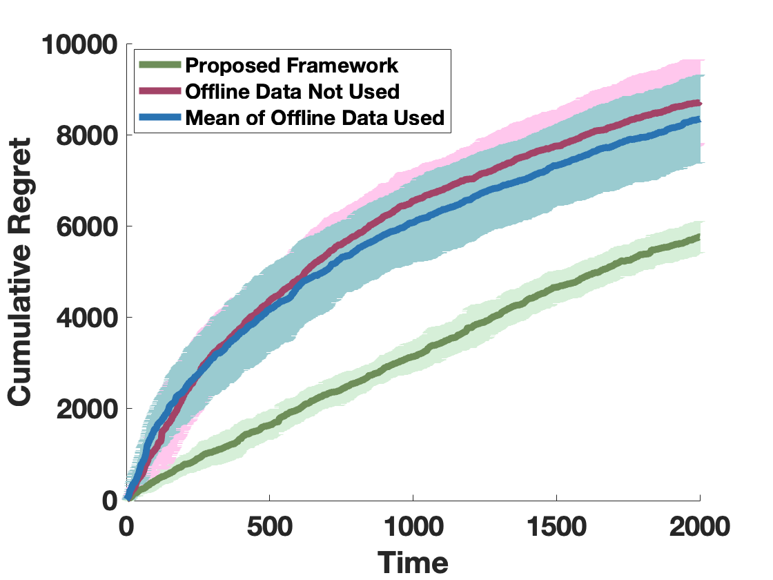
For all of our numerical results, we run $10$ simulations and present the mean and the standard deviation for each scenario. Figure 1 presents the numerical results that compare the cumulative regret of Algorithm 1 for $S=3000$. From Figure 1, the proposed approach outperforms al algorithm that either does not utilize the available data or that only uses $\hat{\theta}^{\text{sim}}$ computed from the offline data, implying that utilizing estimate and the uncertainty from dissimilar systems can be beneficial.

Figure 2 presents the cumulative regret of the proposed Algorithm TSOD-LQR for values of $S=1500,2500,5000$. From Figure 2, the cumulative regret of Algorithm TSOD-LQR decreases as $S$ increases.

We now briefly describe how this framework generalizes to when multiple trajectories $S_{1},\dots,S_{N}$ are available from systems $\theta_{*,1}^{\text{sim}},\dots,\theta_{*,N}^{\text{sim}}$, respectively.

By defining the $l_{2}$-least squares error as

and minimizing with respect to $\theta$ yields

Then, following analogous steps as in the proof of Theorem IV.1, we obtain

With these modifications, we can now utilize Algorithm 1 for online control of LQR when offline data from multiple dissimilar sources are available. By defining $S=\sum_{i=1}^{N}S_{i}$ and $M_{\delta}=\max{M_{\delta,i}}$ and by following analogous steps as in the proof of Theorem V.1, a similar upper bound on the cumulative regret of Algorithm 1 can be obtained.

In this work, we considered an online control problem of an LQR when an offline trajectory of length $S$ of state-action pairs from a similar linear system, also of unknown system matrices, is available. We design and analyze an algorithm that utilizes the available data from the trajectory and establish that the algorithm achieves $\tilde{\mathcal{O}}(f(S,M_{\delta}){\sqrt{T}})$ regret, where $f(S,M_{\delta})$ is a decreasing function of $S$. Finally, we provide additional numerical insights by comparing our algorithm with two other approaches.

We greatly acknowledge the valuable comments by Dr. Gugan Thoppe from the Indian Institute of Science (IISc).

References

- [1] Y. Abbasi-Yadkori and C. Szepesvári, “Regret bounds for the adaptive control of linear quadratic systems,” in Proceedings of the 24th Annual Conference on Learning Theory, pp. 1–26, JMLR Workshop and Conference Proceedings, 2011.
- [2] T. Kargin, S. Lale, K. Azizzadenesheli, A. Anandkumar, and B. Hassibi, “Thompson sampling achieves regret in linear quadratic control,” in Conference on Learning Theory, pp. 3235–3284, PMLR, 2022.
- [3] Y. Ouyang, M. Gagrani, and R. Jain, “Control of unknown linear systems with thompson sampling,” in 2017 55th Annual Allerton Conference on Communication, Control, and Computing (Allerton), pp. 1198–1205, IEEE, 2017.
- [4] A. Cohen, T. Koren, and Y. Mansour, “Learning linear-quadratic regulators efficiently with only regret,” in International Conference on Machine Learning, pp. 1300–1309, PMLR, 2019.
- [5] Y. Li, “Reinforcement learning in practice: Opportunities and challenges,” arXiv preprint arXiv:2202.11296, 2022.
- [6] R. F. Prudencio, M. R. Maximo, and E. L. Colombini, “A survey on offline reinforcement learning: Taxonomy, review, and open problems,” IEEE Transactions on Neural Networks and Learning Systems, 2023.
- [7] W. Zhao, J. P. Queralta, and T. Westerlund, “Sim-to-real transfer in deep reinforcement learning for robotics: a survey,” in 2020 IEEE symposium series on computational intelligence (SSCI), pp. 737–744, IEEE, 2020.
- [8] P. Shivaswamy and T. Joachims, “Multi-armed bandit problems with history,” in Artificial Intelligence and Statistics, pp. 1046–1054, PMLR, 2012.
- [9] C. Zhang, A. Agarwal, H. D. Iii, J. Langford, and S. Negahban, “Warm-starting contextual bandits: Robustly combining supervised and bandit feedback,” in Proceedings of the 36th International Conference on Machine Learning, vol. 97, pp. 7335–7344, PMLR, 2019.
- [10] C. Kausik, K. Tan, and A. Tewari, “Leveraging offline data in linear latent bandits,” arXiv preprint arXiv:2405.17324, 2024.
- [11] B. Hao, R. Jain, T. Lattimore, B. Van Roy, and Z. Wen, “Leveraging demonstrations to improve online learning: Quality matters,” in International Conference on Machine Learning, pp. 12527–12545, PMLR, 2023.
- [12] H. Mania, S. Tu, and B. Recht, “Certainty equivalence is efficient for linear quadratic control,” Advances in Neural Information Processing Systems, vol. 32, 2019.
- [13] D. Baby and Y.-X. Wang, “Optimal dynamic regret in lqr control,” Advances in Neural Information Processing Systems, vol. 35, pp. 24879–24892, 2022.
- [14] T.-J. Chang and S. Shahrampour, “Regret analysis of distributed online lqr control for unknown lti systems,” IEEE Transactions on Automatic Control, 2023.
- [15] M. Abeille and A. Lazaric, “Improved regret bounds for thompson sampling in linear quadratic control problems,” in International Conference on Machine Learning, pp. 1–9, PMLR, 2018.
- [16] T. Guo and F. Pasqualetti, “Transfer learning for lqr control,” arXiv preprint arXiv:2503.06755, 2025.
- [17] T. Guo, A. A. Al Makdah, V. Krishnan, and F. Pasqualetti, “Imitation and transfer learning for lqg control,” IEEE Control Systems Letters, vol. 7, pp. 2149–2154, 2023.
- [18] L. Li, C. De Persis, P. Tesi, and N. Monshizadeh, “Data-based transfer stabilization in linear systems,” IEEE Transactions on Automatic Control, vol. 69, no. 3, pp. 1866–1873, 2023.
- [19] L. Xin, L. Ye, G. Chiu, and S. Sundaram, “Learning dynamical systems by leveraging data from similar systems,” IEEE Transactions on Automatic Control, 2025.
- [20] Y. Abbasi-Yadkori, D. Pál, and C. Szepesvári, “Improved algorithms for linear stochastic bandits,” Advances in neural information processing systems, vol. 24, 2011.
- [21] A. Cassel, A. Cohen, and T. Koren, “Logarithmic regret for learning linear quadratic regulators efficiently,” in International Conference on Machine Learning, pp. 1328–1337, PMLR, 2020.
- [22] I. Osband and B. Van Roy, “Posterior sampling for reinforcement learning without episodes,” arXiv preprint arXiv:1608.02731, 2016.
- [23] Y. Abbasi-Yadkori, D. Pál, and C. Szepesvári, “Online least squares estimation with self-normalized processes: An application to bandit problems,” arXiv preprint arXiv:1102.2670, 2011.