LFTC-24-01/84 -12C states and detailed study of momentum space method for - and -nucleus bound states
Abstract
We perform a detailed study of the -, - and -nucleus systems in momentum space to calculate the bound-state energies and the corresponding coordinate space radial wave functions. A comparison is made among different methods to obtain the partial wave decomposition of meson-nucleus potentials in momentum space, namely, (i) the spherical Bessel transform of the numerically obtained original potential in coordinate space, (ii) the partial wave decomposition of the Fourier transform of the Woods-Saxon approximated form for the original potential, and (iii) the spherical Bessel transform of the Woods-Saxon approximation of the numerically obtained original potential. The strong nuclear bound-state energies for the -4He, -12C, -4He, -12C, -4He (no Coulomb), and -12C (no Coulomb) systems and the corresponding wave functions in coordinate space are compared for the three methods. Furthermore, as an initial and realistic study, the -12C bound states are studied for the first time, with the effects of self-consistently calculated Coulomb potentials in 12C (when the mesons are absent).
I Introduction
Studies of hadron properties under extreme conditions indicate that the Lorentz scalar effective masses of mesons are expected to decrease in a nuclear medium, as a consequence of partial restoration of chiral symmetry Krein:2010vp ; Tsushima:2011kh ; Ko:1992tp ; Asakawa:1992ht . This negative effective mass shift (Lorentz scalar) of the meson can be regarded as an attractive Lorentz scalar potential, and when the sum of the Lorentz scalar and the Lorentz vector potentials (total potential in a nonrelativistic sense) is sufficiently attractive, the mesons can be bound to atomic nuclei. In the case of heavy quarkonia (no vector potentials arise in the lowest order), charmonium-nucleus systems were proposed in 1989 Brodsky:1989jd , which led to various subsequent studies Krein:2010vp ; Tsushima:2011kh ; Hosaka:2016ypm ; Metag:2017yuh ; Krein:2017usp ; Lee:2000csl ; Krein:2013rha ; Klingl:1998sr ; Hayashigaki:1998ey ; Kumar:2010hs ; Belyaev:2006vn ; Yokota:2013sfa ; Peskin:1979va ; Kharzeev:1995ij ; Kaidalov:1992hd ; Luke:1992tm ; deTeramond:1997ny ; Brodsky:1997gh ; Sibirtsev:2005ex ; Voloshin:2007dx ; TarrusCastella:2018php ; Cobos-Martinez:2020ynh and lattice QCD calculations Yokokawa:2006td ; Kawanai:2010ev ; Skerbis:2018lew on these states. Recent lattice results show also a possibility of -nucleon (N) bound states Chizzali:2022pjd , although is not the heavy quarkonium. Furthermore, by the developed Faddeev three-body approach using the lattice extracted -N potential, a possible -NN bound state is predicted Etminan:2024vkv . We have studied further the bottomonium-nucleus systems Krein:2010vp ; Cobos-Martinez:2020ynh , and predicted that the and mesons can form strong nuclear bound states with various nuclei Zeminiani:2020aho ; Zeminiani:2021vaq ; Zeminiani:2021xvw ; Cobos-Martinez:2022fmt , provided that they are produced inside a nucleus with very low relative momenta to the nucleus.
The Okubo-Zweig-Iizuka (OZI) rule dictates the suppression of the light hadron exchange in the heavy quarkonium-nucleus interaction, then the interaction must occur primarily by multigluon exchange, namely, a QCD van der Waals type of interaction Brodsky:1997gh . Looking at different possibilities, we consider an alternative (effective) mechanism for the quarkonium-nucleus interaction. We estimated the charmonia ( and ) and bottomonia ( and ) mass shifts by the enhanced in-medium self-energies via the excitations of intermediate-state hadrons with light quarks Cobos-Martinez:2020ynh .
The focus of the present study is firstly the bottomonia, for which the self-energies were calculated including only the minimal loop contributions for the and mesons, namely, the loop for the , and the loop for the Zeminiani:2020aho . The calculations were performed neglecting any possible imaginary part of the self-energies. Secondly, we study the -nucleus bound states for the first time, with and without the Coulomb force.
To obtain the bound-state energies and the corresponding bound meson state wave functions of the meson-nucleus systems in the coordinate space, we solve the Klein-Gordon equation in momentum space, where for the case, the Proca equation is approximated and reduced to the Klein-Gordon equation assuming the longitudinal and transverse modes are nearly equal with low momentum. It is very convenient to deal with the kinetic term in the Klein-Gordon equation in momentum space, and the search for the bound-state energies is also much more simple than performing in coordinate space. This can be done by solving the differential wave equation as an eigenvalue equation, and using a method for finding selected eigenvalues and eigenfunctions (eigen vectors). This makes it easy to extend the calculation for complex Hamiltonians, e.g., when including the meson widths and/or imaginary potentials. In coordinate space, dealing with complex eigenvalues is tricky, as it involves searching for a convergence point in the real and imaginary parts in energy plane, as well as the real and imaginary parts of the coordinate space wave functions.
The treatment in momentum space requires the nuclear potentials to be transformed from coordinate space to momentum space, and then decomposed into partial waves. For this purpose we compare three different methods, namely, (i) the spherical Bessel transform of the numerically obtained original potential in coordinate space, (ii) the partial wave decomposition of the Fourier transform of the Woods-Saxon approximated form for the original potential, and (iii) the spherical Bessel transform of the Woods-Saxon approximation of the numerically obtained original potential.
The bound-state energies calculated for -12C, -4He, -12C and -4He systems reported in Cobos-Martinez:2022fmt are reproduced here and compared with new values obtained through the different methods mentioned above, for which we now present for the first time the wave functions in coordinate space associated with each energy level of the bound state. In this article we also include the first calculation of the -nucleus bound states, for -4He and -12C with no Coulomb interaction, followed by a realistic study of -12C including the Coulomb potentials, which are obtained self-consistently in the 12C nucleus when the mesons are absent, within the quark-meson coupling (QMC) model treatment for finite nuclei Guichon:1987jp ; Guichon:1995ue ; Tsushima:2002cc ; Tsushima:1997df ; Saito:1996sf ; Saito:2005rv .
This article is organized as follows. In Sec. II we discuss different methods used to solve the Klein-Gordon equation in momentum space. The numerical procedure of the calculation is explained in Sec. III, and the results are presented in Sec. IV. An initial study of the -4He (no Coulomb potential) and -12C bound states (with and without the Coulomb potentials) is made in Sec. V. The summary and conclusions are given in Sec. VI.
II Formulation in momentum space
The meson-nucleus bound states are studied in momentum space by solving the Klein-Gordon (K.G.) equation. While the K.G. equation is solved for the pseudoscalar meson, we also solve the K.G. equation for the spin-1 meson. This is based on the approximation that the -nucleus relative momentum is nearly zero. In this approximation, the transverse and longitudinal components in the Proca equation are expected to be very similar, which allows us to reduce it to solving a single-component K.G. equation, as practiced in Ref. Zeminiani:2021vaq ; Zeminiani:2021xvw ; Cobos-Martinez:2022fmt .
The - and -nuclear potentials were previously calculated in coordinate space in Ref. Cobos-Martinez:2022fmt , in which they were transformed into the momentum-space by one particular method for that study (“Woods-Saxon Fourier transform” method to be explained later). For the purpose of the present study, we will transform the coordinate space potentials using a few methods, including the same method used in the past.
The K.G. equation will be solved for each value of the angular momentum of the meson-nucleus system to calculate the bound-state energies and to get the momentum space eigen wave function corresponding to each bound state energy level of the system. This will require a partial wave decomposition for either the momentum-space or the coordinate-space potentials. We will compare three different methods to obtain the partial-wave decomposed momentum-space potentials.
II.1 Klein-Gordon equation
We solve the K.G. equation in momentum space of the form
| (1) |
where is the reduced mass of the meson-nucleus system (, is the meson mass and the nucleus mass) and and are the Lorentz scalar and vector potentials, respectively. The vector potentials are such as the Coulomb potential , and the nuclear vector potentials, where the nuclear potentials generally contain a scalar () and vector ( and ) potentials. In this article, we will denote the nuclear mean field potentials as , where the vector -mean field potentials are canceled when calculating the botomonium- and -nucleus potentials (or when they have no light quarks) in the present approach and thus we do not need -mean field potentials in the following, and the very small isovector -mean field potentials, that are proportional to the difference of the proton and neutron densities (isovector nuclear density) in nuclei, are also canceled in calculating the bottomonium- and -nucleus potentials (or, again, when they have no light quarks) in the present approach. Detailed explanations follow next.
For and mesons, the nuclear potential arises from the intermediate state excitations of mesons containing light quarks in the self-energy, namely, the and mesons interacting with a nucleus (with the surrounding nuclear medium). We have estimated this interaction with the extended treatment of the original QMC model Guichon:1987jp , which has been successfully applied for various studies in nuclear matter and nuclei Guichon:1995ue ; Tsushima:2002cc ; Tsushima:1997df ; Saito:1996sf ; Saito:2005rv ; Tsushima:2019wmq ; Krein:2010vp ; Krein:2017usp . In the QMC model, the light quarks in the and mesons interact with the light quarks in the nucleons in a nucleus through the (scalar-isoscalar), (vector-isoscalar) and (vector-isovector) fields. But the and mean field potentials for the light quarks and antiquarks of () and () cancel out (for more details, see Zeminiani:2020aho ). For this reason, the bottomonium-nucleus potential is treated as only containing the attractive scalar mean field potential,
| (2) |
while for the mesons we will include the (vector) Coulomb potentials in realistic cases in Sec. V.
II.2 Nuclear potentials
II.2.1 Originally calculated potentials
The coordinate-space nuclear potentials for the systems -4He, -12C, -4He and -12C are calculated using a local density approximation. For a bottomonium (=,) and a nucleus , the potential is given by the equation
| (3) |
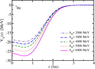
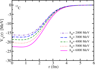
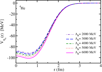
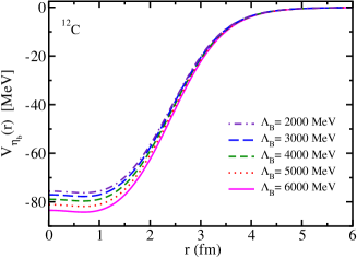
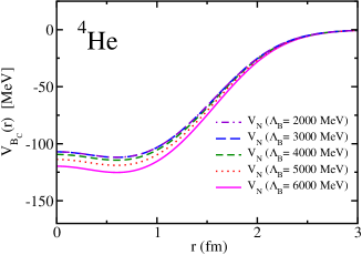
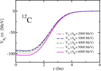
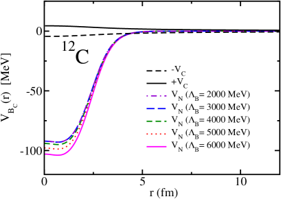
where is the distance from the center of the nucleus, is the meson mass shift (Lorentz scalar), being the in-medium effective or mass in nuclear matter, and is the nuclear density distribution in the nucleus . For the 12C nucleus, it was calculated by the QMC model Saito:1996sf , and for the 4He nucleus we use the parameterized nuclear density from Ref. Saito:1997ae . The value of the mass shift is dependent on the cutoff mass parameter that appears in the form factor used to regularize the meson self-energy Zeminiani:2020aho . Thus, the results obtained in this study depend on the values of this cutoff, as shown in Fig. 1.
II.2.2 Woods-Saxon potential form parametrization
In order to use conveniently the approximated form for the calculated quarkonium-nucleus potentials shown in Fig. 1, we adopt the Woods-Saxon potential form which is commonly used to approximately parameterize nuclear potentials,
| (4) |
where is the potential depth, is the nuclear radius and is the surface thickness of the nucleus. These parameters will be determined by the fit for each nucleus for a given numerically obtained original potential.
The use of the Woods-Saxon form parameterized potential enables us to work with an analytical form of . This is done by interpolating the numerical data to fit to the Woods-Saxon shape. The obtained parameters for each potential are presented in Table 1. The advantage of using the Woods-Saxon potential form is that, one does not need to be provided with the obtained original numerical potential data, but just may know the Woods-Saxon potential parameters.
| Woods-Saxon potential parameter values | ||||
|---|---|---|---|---|
| MeV | MeV | MeV | ||
| (MeV) | 19.83 | 22.84 | 27.54 | |
| (fm) | 1.6199 | 1.6215 | 1.6237 | |
| (fm) | 0.2832 | 0.2833 | 0.2835 | |
| (MeV) | 16.66 | 19.21 | 23.20 | |
| (fm) | 2.4638 | 2.4662 | 2.4692 | |
| (fm) | 0.4805 | 0.4806 | 0.4808 | |
| (MeV) | 91.84 | 95.91 | 101.42 | |
| (fm) | 1.6351 | 1.6352 | 1.6353 | |
| (fm) | 0.28445 | 0.28446 | 0.28447 | |
| (MeV) | 77.82 | 81.28 | 85.96 | |
| (fm) | 2.4854 | 2.4856 | 2.4858 | |
| (fm) | 0.48181 | 0.48182 | 0.48183 | |
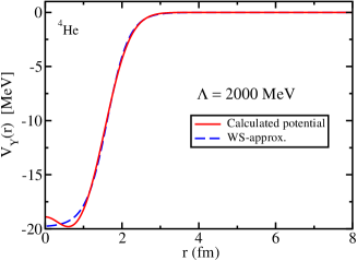
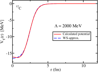
A comparison between the numerically obtained original potentials and the corresponding fitted Woods-Saxon form potentials is made in Fig. 2 for and for the case of MeV. One can easily observe that the fitted Woods-Saxon form potentials are good approximations of the original potentials, and the differences in the calculated bound state energies using the parametrized potentials are expected to be small (indeed, this will be demonstrated later).
II.3 Partial wave decomposition
The partial wave solutions for the bound state energies and the corresponding wave functions of the K.G equation require the decomposition of the meson-nucleus potential into a given angular momentum -wave. There are at least a few ways of obtaining such -wave potentials, of which we will test three methods: (i) The direct spherical Bessel transform of the originally obtained numerical potential data, (ii) the decomposition of the analytical Fourier transform of the Woods-Saxon form potential, and (iii) the direct spherical Bessel transform of the Woods-Saxon fitted potential.
II.3.1 Double spherical Bessel transform
Generally, a straightforward way to obtain the -wave decomposition of the meson-nucleus potential is to apply the double spherical Bessel transform,
| (5) |
where ( = 0, 1, 2, …) are the spherical Bessel functions. (The reason why the potential has two arguments and (as well as in the next section and ) will become clearer in Sec. III.) This transformation is applied on both the original potential from data and its fitted Woods-Saxon potential.
Since this transformation contains spherical Bessel functions, the oscillatory behaviour of these functions must be tamed properly in order to construct the wave function in momentum space, as well as when the momentum space wave function is transformed to the coordinate space for each partial wave solution. This is achieved by tuning the and grids to construct suitable discrete sets. More explanations on this will be given in a later section.
II.3.2 Fourier transform of the fitted Woods-Saxon form potential
Alternatively, the Fourier transform of the Woods-Saxon form potential of Eq. (4) can be carried out analytically using complex analysis. After the integration in the complex plane, we end up with the following equation,
| (6) | |||||
with , and . The value of does not affect significantly the final result, since the first few terms in the sum already gives nearly a converged result, and thus = 4 or 5 is sufficient.
The partial wave -projected potentials in momentum space are then calculated by
| (7) |
where are the Legendre polynomials of -th order and is the angle between and . After the Fourier transform is performed analytically, the partial wave decomposition is made numerically.
III Numerical Procedure
The partial wave expansion of Eq. (2) is given by
| (8) | |||||
The discretized Eq. (8) can be written in matrix form as
| (9) |
where . The matrix elements of the Hamiltonian are
| (10) |
with being the number of points for the momentum grid, and and are respectively the -th momentum point and -th weight.
Equation (9) can be solved as an eigenvalue equation using iterative methods, such as the inverse iteration Heddle:1985dh . It is a method for finding selected eigenvalues and eigenfunctions, that has the advantage of only requiring the inversion of an matrix. The equation to be solved is of the type
| (11) |
We begin with some guess value , and constructing the operator
| (12) |
that contains the Hamiltonian of Eq. (11). Next, we construct a state that can be expressed using the complete set of eigenfunctions
| (13) |
which is multiplied times by the operator , resulting in
| (14) |
For nondegenerate eigenstates and for a proper guess , will rapidly take over the sum. Then, for a large enough N
| (15) |
which can be written in a momentum space calculation as
| (16) |
To facilitate the iterative numerical calculation, is divided by its element with maximum modulus, , and is redefined as
| (17) |
and for sufficiently large ,
| (18) |
The eigenvalue is then given by
| (19) |
In the same way, the eigenvector is determined by Eq. (18). The obtained eigenvalue and eigenvector are the system’s eigenenergy and momentum space wave function, respectively, for each and .
III.1 Selection of gridpoints
There are two sets of gridpoints used to perform the numerical calculations: The and the gridpoints. These points must be properly chosen to be able to perform correctly the Gaussian integrations in Eqs. (5), (7), and (10). In particular, the choice of grid in momentum space is not trivial compared to that in coordinate space, and one needs some care.
For the double spherical Bessel transform, one is recommended to properly limit the maximum number of points, so that the spherical Bessel functions, depending on both and grids, do not cause many oscillations. This is necessary to obtain the stable and nonexcessively oscillating wave functions (more explanations later). Furthermore, the grid should contain the proper and sufficient points in the region where the potential is relevant. For example, the potentials presented in Fig. 1 are relevant in the region from = 0 fm up to = 2 or 3 fm. This means that most of the gridpoints should be in this region close to the center of the nucleus, leaving less points to the region outside of this. A good choice for the momentum gridpoints in this integration is found to be .
When constructing the Hamiltonian, however, the distribution of points is not necessarily the same as when performing the spherical Bessel transform. This is because of the kinetic term in the Hamiltonian. When transforming the potential to the momentum space, one should consider primarily the points where the potential is relevant, whereas in constructing the Hamiltonian of the system, Eq. (10), the points in the momentum corresponding to the regions in coordinate space further away from the center of nucleus must also be included. We use the points following Ref. Kwon:1978tz , where are the Gaussian points defined in the region .
IV Results
IV.1 Bound-state energies
After solving numerically Eq. (9), we can obtain the bound-state energies of the meson-nucleus system, that are given by . The results are presented in Tables 2 and 3 for the different methods of partial wave decomposition and cutoff values. We have obtained the energy levels by varying the eigenvalue initial guess, , for fixed . To get each eigenvalue, a different initial guess value is chosen, and this is repeated until all the desired energy levels are obtained. Each converged eigenvalue is then confirmed by analysing the number of nodes in the corresponding coordinate space wave function. (Detailed explanations are given in next subsection.) Note that, the obtained bound state energies for 1s and 1p by the ”Woods-Saxon Fourier transform” sometimes may deviate about several MeV from those obtained by the ”Direct Bessel transform” and ”Woods-Saxon Bessel transform” (see Refs. Cobos-Martinez:2020ynh ; Cobos-Martinez:2022fmt ), however, the conclusion on the existence of these states remain the same.
| Bound state energies (MeV) | ||||
| Direct Bessel transform | ||||
| 1s | -5.93 | -6.25 | -6.56 | |
| 1s | -13.22 | -15.26 | -18.41 | |
| 1p | -8.30 | -9.57 | -11.51 | |
| Woods-Saxon Fourier transform | ||||
| 1s | -5.48 | -7.4 | -10.6 | |
| 1s | -10.51 | -12.67 | -16.1 | |
| 1p | -5.95 | -7.79 | -10.78 | |
| Woods-Saxon Bessel transform | ||||
| 1s | -6.35 | -6.75 | -7.14 | |
| 1s | -13.18 | -15.22 | -18.37 | |
| 1p | -8.18 | -9.43 | -11.33 | |
| Bound state energies (MeV) | ||||
| Direct Bessel transform | ||||
| 1s | -68.71 | -71.59 | -75.44 | |
| 1p | -39.97 | -41.50 | -43.54 | |
| 1d | -37.73 | -39.56 | -42.03 | |
| 2s | -29.14 | -30.09 | -31.38 | |
| 1s | -63.70 | -66.93 | -70.27 | |
| 1p | -53.17 | -55.13 | -59.38 | |
| 1d | -46.47 | -48.50 | -51.17 | |
| 2s | -34.53 | -36.30 | -39.43 | |
| 1f | -26.56 | -28.09 | -29.97 | |
| 2p | -18.86 | -20.67 | -23.15 | |
| Woods-Saxon Fourier transform | ||||
| 1s | -63.1 | -66.7 | -71.5 | |
| 1p | -40.6 | -43.7 | -48.0 | |
| 1d | -17.2 | -19.7 | -23.2 | |
| 2s | -15.6 | -17.9 | -21.1 | |
| 1s | -65.8 | -69.0 | -73.4 | |
| 1p | -57.0 | -60.1 | -64.3 | |
| 1d | -47.5 | -50.4 | -54.4 | |
| 2s | -46.3 | -49.1 | -53.0 | |
| 1f | -37.5 | -40.2 | -43.9 | |
| 2p | -36.0 | -38.6 | -42.2 | |
| Woods-Saxon Bessel transform | ||||
| 1s | -67.79 | -70.65 | -74.48 | |
| 1p | -40.42 | -41.95 | -43.99 | |
| 1d | -36.46 | -38.23 | -40.64 | |
| 2s | -28.67 | -29.60 | -30.85 | |
| 1s | -63.41 | -66.05 | -69.59 | |
| 1p | -52.90 | -55.44 | -58.87 | |
| 1d | -46.34 | -48.35 | -51.05 | |
| 2s | -34.12 | -36.41 | -39.54 | |
| 1f | -26.90 | -28.29 | -30.18 | |
| 2p | -18.72 | -20.53 | -23.02 | |
IV.2 Coordinate-space wave functions
From the eigenvectors that come out as solutions of Eq. (9), we can use a (single) spherical Bessel transform to obtain the coordinate-space wave functions of the corresponding energy levels of the system:
| (20) |
where the normalization is performed in according to the convention (recall that the wave functions are real in the present study),
| (21) |
As commented already, this procedure enables us to confirm that the obtained eigen energies are indeed corresponding to the correct eigen wave functions.
The gridpoints used in this integration may better be the same as those used to obtain the partial wave decomposition of the nuclear potential, namely the same as those when performing the double spherical Bessel transform. Otherwise the resultant wave function would be often unstable, with exceeding oscillations. We have observed that, the more the grid points differ from the corresponding points used for the partial wave decomposition, the more oscillations in the wave function are. For this reason, when one performs the spherical Bessel transform of the potential, one needs to chose properly the gridpoints that result in a smooth wave function.
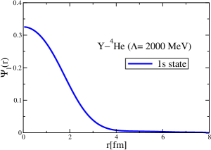
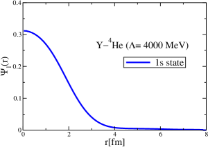
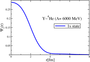
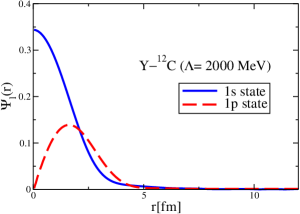
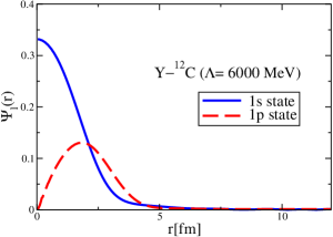
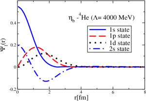
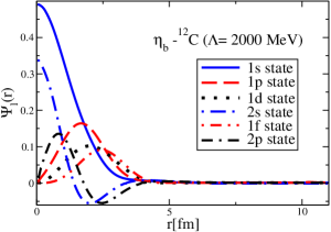
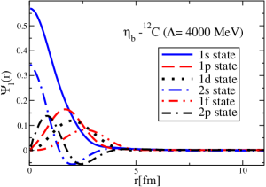
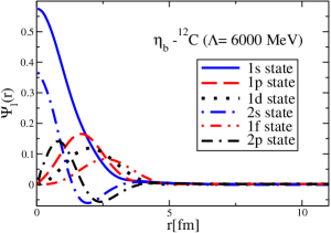
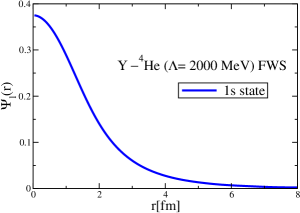
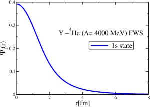
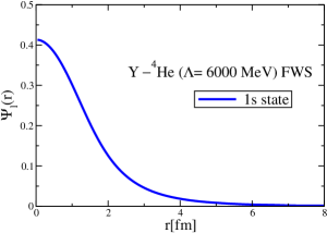
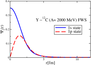
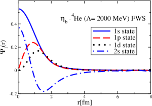
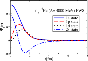
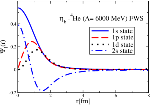
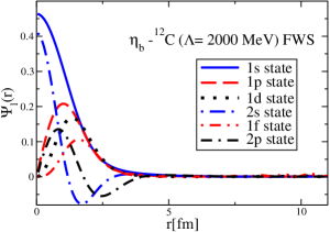
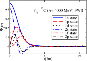
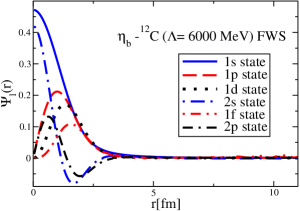
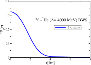
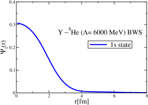
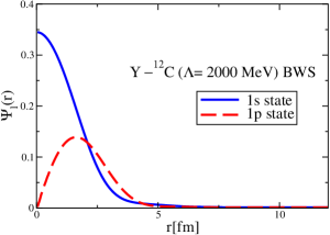
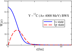
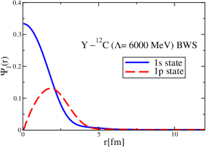
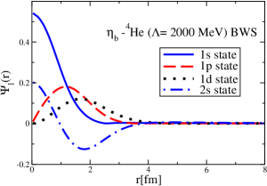
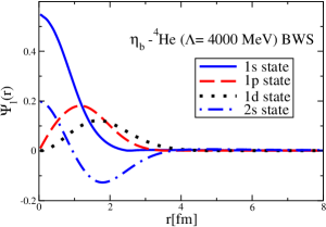
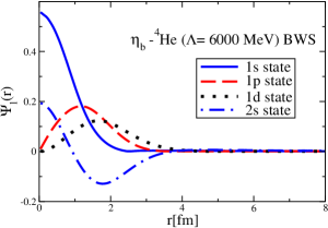
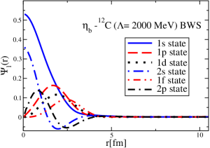
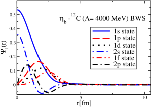
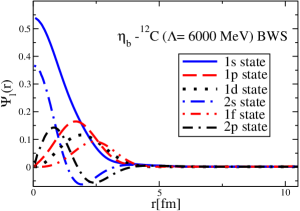
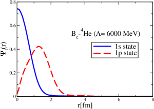
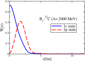
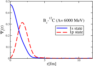
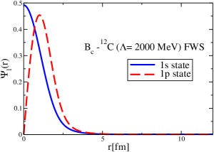
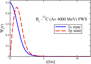
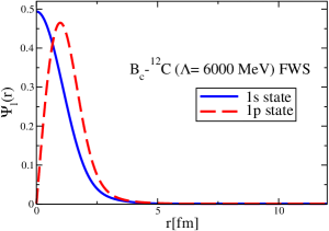
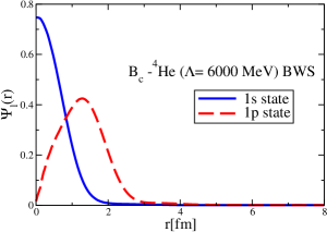
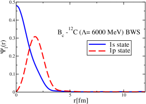
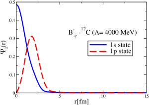
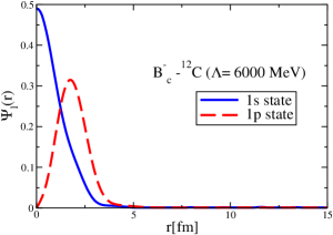
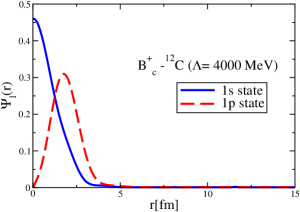
The results for the -4He, -12C, -4He and -12C wave functions, for different methods of partial-wave decomposition and cutoff values, are presented in Figs. 3 to 14.
The wave functions obtained when using the Bessel transform of the original potential and its fitted Woods-Saxon form are very similar in all energy levels. The decomposition of the Fourier transform of the fitted Woods-Saxon potential, however, produces different shapes of wave functions, more notably when comparing the wave function distributions for various energy levels. Thus, the method used for finding the partial wave decomposition of the momentum space potential significantly affects the shapes of wave functions, as it does for the bound-state energy outputs.


V Initial study of the -4He and -12C bound states with and without the Coulomb potentials
After establishing and confirming the momentum-space methods by three different ways, as well as to obtain the wave functions in the coordinate space, we now proceed to an initial study of the -4He and -12C bound states. The mass shift of meson in symmetric nuclear matter was calculated in Ref. Zeminiani:2023gqc , and we obtain the -nucleus strong potential using a local density approximation. For a realistic calculation, the Coulomb potentials should enter for -nucleus potentials, but they are absent in the and cases. First, we include only the strong interaction part of the -4He and -12C potentials, without the Coulomb potentials. Second, including the Coulomb potentials, we study the -12C bound states, and focus on the role of the Coulomb potentials. This is because the 12C nucleus is constructed self-consistently by the QMC model (relativistic, quark-based nuclear shell model), but this is not done for the 4He nucleus.
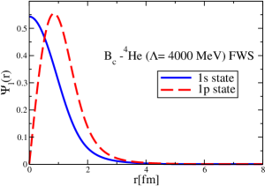
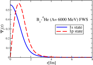
The strong interaction potentials for are presented in Fig. 15. These are calculated in the same manner as those for the and cases. The parametrization of the fitted Woods-Saxon form of these potentials is given in Table. 4. We solve the K.G. equation with the three methods mentioned previously and obtain the bound-state energies, which we present in Table 5. The corresponding wave functions are shown in Figs. 16 to 21.
| Woods-Saxon potential parameter values | ||||
|---|---|---|---|---|
| MeV | MeV | MeV | ||
| (MeV) | 112.12 | 114.61 | 125.45 | |
| (fm) | 1.6308 | 1.6311 | 1.6307 | |
| (fm) | 0.28427 | 0.2843 | 0.28426 | |
| (MeV) | 94.77 | 96.90 | 106.04 | |
| (fm) | 2.4796 | 2.4801 | 2.4795 | |
| (fm) | 0.48167 | 0.4817 | 0.48166 | |
| Bound state energies (MeV) | ||||
| Direct Bessel transform | ||||
| 1s | -75.14 | -76.67 | -83.14 | |
| 1p | -42.06 | -42.91 | -46.43 | |
| 1s | -74.55 | -76.06 | -82.43 | |
| 1p | -51.53 | -52.88 | -58.64 | |
| Woods-Saxon Fourier transform | ||||
| 1s | -78.04 | -80.22 | -89.68 | |
| 1p | -51.42 | -53.34 | -61.68 | |
| 1s | -79.67 | -81.65 | -90.14 | |
| 1p | -68.62 | -70.50 | -78.57 | |
| Woods-Saxon Bessel transform | ||||
| 1s | -74.10 | -75.53 | -82.09 | |
| 1p | -42.43 | -43.26 | -46.75 | |
| 1s | -74.31 | -75.83 | -82.21 | |
| 1p | -51.79 | -53.19 | -58.93 | |


We now study the more realistic case for the -12C, where we include the Coulomb interaction. Including the Coulomb potential in Eq. (1), it becomes
| (22) |
and the Hamiltonian for the numerical calculation in Eq. (10) now becomes
| (23) | |||||
The Coulomb potentials in the 12C nucleus (nucleon density distribution and Coulomb mean field) is obtained within the QMC model Saito:1996sf self-consistently. We show the Coulomb potentials side-by-side with the nuclear potentials for this nucleus in Fig. 22. Since the mean-field approximation of the QMC model is not good for a light nucleus such as the 4He, we do not investigate the -4He system with the Coulomb potentials in this initial study. In the near future, we plan to include the Coulomb potentials for the -4He system with a different approach, although the effects are expected to be small.
The treatment of the Coulomb potential in momentum space is known to be difficult due to the logarithmic singularity that appears in its partial wave decomposition, requiring the use of some regularization technique, such as the Lande subtraction method Heddle:1985dh ; Kwan:1978zh . In this calculation, however, the treatment is much more simple. The reason is that we can calculate the -12C Coulomb potentials in coordinate space using the self-consistent mean Coulomb field in the 12C nucleus by neglecting the feedback of the Coulomb force from (which should give very small effects). Thus, we simply get the direct partial wave decomposition of the Coulomb potentials in momentum space according to the methods already explained in Sec. II.3.
We solve Eq. (22) using the direct double spherical Bessel transform for the following cases: (i) Nuclear and attractive Coulomb potentials (-12C), (ii) nuclear and repulsive Coulomb potentials (-12C)), (iii) only nuclear potentials, (iv) only Coulomb potentials, and (v) the cases of the term in the right hand side of Eq. (22), in the right hand of the expansion, (see Eq. (23) with ). The results are presented in Table 6. We make this comparison to see the interference effect between the dominant nuclear and Coulomb potentials, which arises naturally for the relativistic K.G. equation case but not for the lowest order Schrödinger equation. Solving Eq. (22) for , and the Coulomb potential alone, we get energies, MeV for , with a small asymmetry between the cases of the attractive and repulsive Coulomb potentials, that arises from the term and diminishes the energy in both cases. Naively one could expect that the bound-state energies obtained including the nuclear and attractive (or repulsive) Coulomb potentials to be around 1.4 MeV deeper (or shallower) than the case of the nuclear potential alone, however, in fact we obtain more than 3 to 4 MeV difference for the 1s state. This happens because the nuclear potential dominates in the term that appears when we include the Coulomb potential. The ”interference” between the nuclear and Coulomb potentials is responsible for this larger difference. By making the term , we nearly recover the energies found for the case of only nuclear interaction, aside from a small difference due to the term. This shows that when including the Coulomb interaction, the nuclear potential dominates , as one can expect. Although the Coulomb effect is small, such behavior described above cannot be seen in a naive treatment using the Schrödinger equation without including up to the term.
| Bound state energies (MeV) | ||||
| -12C (Strong only) | ||||
| 1s | -74.55 | -76.06 | -82.43 | |
| 1p | -51.53 | -52.88 | -58.64 | |
| -12C | ||||
| 1s | -79.12 | -80.63 | -87.03 | |
| 1p | -56.15 | -57.53 | -63.38 | |
| -12C () | ||||
| 1s | -75.06 | -76.58 | -82.98 | |
| 1p | -52.63 | -54.01 | -59.85 | |
| -12C | ||||
| 1s | -71.01 | -72.53 | -78.94 | |
| 1p | -49.11 | -50.49 | -56.32 | |
| -12C (Coulomb only) | ||||
| -12C | -12C () | -12C | ||
| 1s | -1.43 | -0.01 | +1.46 | |
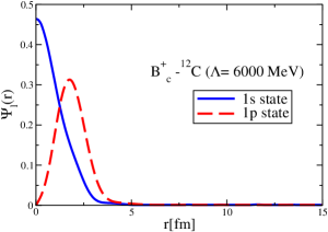
The coordinate space wave functions for the 1s and 1p states for the -12C system are presented in Fig. 23.


VI Summary and Conclusion
By solving the Klein-Gordon equation in momentum space, we have calculated the single-particle energies and the corresponding coordinate-space wave functions for the quarkonium-nucleus systems, for the and mesons and the 4He and 12C nuclei. The meson-nucleus potentials have been calculated from the mass shift of the mesons in nuclear matter using a local density approximation without the effects of the meson widths. The results depend on the cutoff parameter values, introduced in the regularization of the meson self-energies.
We have studied and compared in detail the momentum space methods for solving the Klein-Gordon equation, as well as the resultant coordinate space wave functions by three methods to construct the momentum-space potentials: (i) double spherical Bessel transform of the numerically obtained coordinate-space original potential, (ii) Fourier transform of the fitted Woods-Saxon form potential in the coordinate space, and (iii) double spherical Bessel transform of the fitted Woods-Saxon form potential in the coordinate space.
When using the double spherical Bessel transform, the choice of a suitable momentum grid is crucial to guarantee the corresponding proper coordinate space regions where the potential is relevant.
It is important to use the same momentum grid when transforming the momentum-space wave function into the coordinate space in order to obtain a stable, smooth and proper wave function. Furthermore, there is no need to interpolate.
The double spherical Bessel transform of the fitted Woods-Saxon form potential in the coordinate-space yields nearly the same results for the bound-state energies and coordinate space wave functions. Thus, we can provide the corresponding parameter sets of the fitted Woods-Saxon form potentials, instead of the original meson-nucleus potentials obtained numerically.
We also have calculated for the first time the -4He and -12C bound-state energies and coordinate space wave functions, with only the strong interaction potentials first, and then, for -12C system, we have studied including the realistic Coulomb potentials, and analyzed the ”interference” effect between the nuclear and Coulomb potentials.
In the future, more realistic studies can be made for the -, - and -nucleus systems for various nuclei, including the possible imaginary part of the potentials for the -, - and -nucleus bound states. In particular, the realistic Coulomb potentials will be included for the - and -nucleus systems.
Acknowledgements.
The authors acknowledge the support and warm hospitality of APCTP (Asia Pacific Center for Theoretical Physics) during the Workshop (APCTP PROGRAMS 2023) ”Origin of Matter and Masses in the Universe: Hadrons in free space, dense nuclear medium, and compact stars”, where important discussions and development were achieved on the topic. The authors also thank the OMEG (Origin of Matter and Evolution of Galaxies) Institute at Soongsil University for the supports in many aspects during the collaboration visit in Korea. The authors thank A. W. Thomas for his useful comments on the coordinate space wave functions at the initial stage of the study and fruitful discussions on this topic. G.N.Z. was supported by the Coordenação de Aperfeiçoamento de Pessoal de Nível Superior- Brazil (CAPES). JJCM acknowledges financial support from the University of Sonora under grant USO315009105. K.T. was supported by Conselho Nacional de Desenvolvimento Científico e Tecnológico (CNPq, Brazil), Processes No. 313063/2018-4, No. 426150/2018-0, and No. 304199/2022-2, and FAPESP Process No. 2019/00763-0 and No. 2023/073-3-6 (G.N.Z. and K.T.). The work of G.N.Z and K.T. was in the projects of Instituto Nacional de Ciência e Tecnologia - Nuclear Physics and Applications (INCT-FNA), Brazil, Process No. 464898/2014-5.References
- (1) G. Krein, A. W. Thomas and K. Tsushima, Phys. Lett. B 697 (2011), 136.
- (2) K. Tsushima, D. H. Lu, G. Krein and A. W. Thomas, Phys. Rev. C 83 (2011), 065208.
- (3) C. M. Ko, P. Levai, X. J. Qiu and C. T. Li, Phys. Rev. C 45 (1992), 1400.
- (4) M. Asakawa, C. M. Ko, P. Levai and X. J. Qiu, Phys. Rev. C 46 (1992) R1159.
- (5) S. J. Brodsky, I. A. Schmidt and G. F. de Teramond, Phys. Rev. Lett. 64 (1990), 1011.
- (6) A. Hosaka, T. Hyodo, K. Sudoh, Y. Yamaguchi and S. Yasui, Prog. Part. Nucl. Phys. 96 (2017), 88.
- (7) V. Metag, M. Nanova and E. Y. Paryev, Prog. Part. Nucl. Phys. 97 (2017), 199.
- (8) G. Krein, A. W. Thomas and K. Tsushima, Prog. Part. Nucl. Phys. 100 (2018), 161.
- (9) S. H. Lee and C. M. Ko, Phys. Rev. C 67 (2003), 038202.
- (10) G. Krein, J. Phys. Conf. Ser. 422 (2013), 012012.
- (11) F. Klingl, S. s. Kim, S. H. Lee, P. Morath and W. Weise, Phys. Rev. Lett. 82 (1999), 3396; 83 (1999), 4224.
- (12) A. Hayashigaki, Prog. Theor. Phys. 101 (1999), 923.
- (13) A. Kumar and A. Mishra, Phys. Rev. C 82 (2010), 045207.
- (14) V. B. Belyaev, N. V. Shevchenko, A. I. Fix and W. Sandhas, Nucl. Phys. A 780 (2006), 100.
- (15) A. Yokota, E. Hiyama and M. Oka, PTEP 2013 (2013), 113D01.
- (16) M. E. Peskin, Nucl. Phys. B 156 (1979), 365.
- (17) D. Kharzeev, Proc. Int. Sch. Phys. Fermi 130 (1996), 105.
- (18) A. B. Kaidalov and P. E. Volkovitsky, Phys. Rev. Lett. 69 (1992), 3155.
- (19) M. E. Luke, A. V. Manohar and M. J. Savage, Phys. Lett. B 288 (1992), 355.
- (20) G. F. de Teramond, R. Espinoza and M. Ortega-Rodriguez, Phys. Rev. D 58 (1998), 034012.
- (21) S. J. Brodsky and G. A. Miller, Phys. Lett. B 412 (1997), 125.
- (22) A. Sibirtsev and M. B. Voloshin, Phys. Rev. D 71 (2005), 076005.
- (23) M. B. Voloshin, Prog. Part. Nucl. Phys. 61 (2008), 455.
- (24) J. Tarrús Castellà and G. Krein, Phys. Rev. D 98 (2018), 014029.
- (25) J. J. Cobos-Martínez, K. Tsushima, G. Krein and A. W. Thomas, Phys. Lett. B 811 (2020), 135882.
- (26) K. Yokokawa, S. Sasaki, T. Hatsuda and A. Hayashigaki, Phys. Rev. D 74 (2006), 034504.
- (27) T. Kawanai and S. Sasaki, Phys. Rev. D 82 (2010), 091501.
- (28) U. Skerbis and S. Prelovsek, Phys. Rev. D 99 (2019), 094505.
- (29) E. Chizzali, Y. Kamiya, R. Del Grande, T. Doi, L. Fabbietti, T. Hatsuda and Y. Lyu, Phys. Lett. B 848 (2024), 138358.
- (30) F. Etminan and A. Aalimi, [arXiv:2402.06914 [nucl-th]].
- (31) G. N. Zeminiani, J. J. Cobos-Martinez and K. Tsushima, Eur. Phys. J. A 57, 259 (2021).
- (32) G. N. Zeminiani, [arXiv:2201.09158 [nucl-th]].
- (33) G. Zeminiani, J. J. Cobos-Martínez and K. Tsushima, PoS PANIC2021 (2022), 208.
- (34) J. J. Cobos-Martínez, G. N. Zeminiani and K. Tsushima, Phys. Rev. C 105, 025204 (2022).
- (35) P. A. Guichon, Phys. Lett. B 200, 235 (1988).
- (36) P. A. M. Guichon, K. Saito, E. N. Rodionov and A. W. Thomas, Nucl. Phys. A 601, 349 (1996).
- (37) K. Tsushima and F. Khanna, Phys. Lett. B 552, 138 (2003).
- (38) K. Tsushima, K. Saito, A. W. Thomas and S. V. Wright, Phys. Lett. B 429, 239 (1998); Phys. Lett. B 436, 453(E) (1998).
- (39) K. Saito, K. Tsushima and A. W. Thomas, Nucl. Phys. A 609, 339 (1996).
- (40) K. Saito, K. Tsushima and A. W. Thomas, Prog. Part. Nucl. Phys. 58, 1 (2007).
- (41) K. Tsushima, AAPPS 29, 37 (2019).
- (42) K. Saito, K. Tsushima and A. W. Thomas, Phys. Rev. C 56, 566 (1997).
- (43) D. P. Heddle, Y. R. Kwon and F. Tabakin, Comput. Phys. Commun. 38, 71 (1985).
- (44) G. N. Zeminiani, S. L. P. G. Beres and K. Tsushima, “In-medium mass shift of two-flavored heavy mesons, , , , , and ,” [arXiv:2401.00250 [hep-ph]].
- (45) Y. R. Kwon, PhD. Theis, UMI-79-17481.
- (46) Y. R. Kwan and F. Tabakin, Phys. Rev. C 18, 932 (1978).