Lifespan estimates for semilinear wave equations with space dependent damping and potential

Ning-An Lai Institute of Nonlinear Analysis and Department of Mathematics
Lishui University
Lishui 323000, P. R. China ninganlai@lsu.edu.cn , Mengyun Liu^∗ Department of Mathematics
Zhejiang Sci-Tech University
Hangzhou 310018, P. R. China mengyunliu@zstu.edu.cn , Ziheng Tu School of Data Science, Zhejiang University of Finance and Economics, 310018 Hangzhou, P. R. China tuziheng@zufe.edu.cn and Chengbo Wang School of Mathematical Sciences
Zhejiang University
Hangzhou 310027, P. R. China wangcbo@zju.edu.cn

Abstract.

In this work, we investigate the influence of general damping and potential terms on the blow-up and lifespan estimates for energy solutions to power-type semilinear wave equations. The space-dependent damping and potential functions are assumed to be critical or short range, spherically symmetric perturbation. The blow up results and the upper bound of lifespan estimates are obtained by the so-called test function method. The key ingredient is to construct special positive solutions to the linear dual problem with the desired asymptotic behavior, which is reduced, in turn, to constructing solutions to certain elliptic “eigenvalue” problems.

Key words and phrases:

semilinear wave equations, damping, potential, lifespan estimate, test function

2010 Mathematics Subject Classification:

35L05, 35L71, 35B33, 35B44, 35B40, 35B30

* Corresponding author

1. Introduction

The purpose of this paper is to investigate the influence of general damping and potential terms on the blow-up and lifespan estimates for energy solutions to power-type semilinear wave equations. The space-dependent damping and potential functions are assumed to be critical or short range, spherically symmetric perturbation.

More precisely, let $n\geq 2$ , $p>1$ , $D,V\in C(\mathbb{R}^{n}\backslash\{0\})$ , we consider the following Cauchy problem of semilinear wave equations, with small data

(1.1)

\left\{\begin{aligned} &u_{tt}-\Delta u+D(x)u_{t}+V(x)u=|u|^{p},(t,x)\in(0,T)\times\mathbb{R}^{n},\\ &u(x,0)=\varepsilon f(x),\quad u_{t}(x,0)=\varepsilon g(x)\end{aligned}\right.

Here $f,g\in C^{\infty}_{c}(\mathbb{R}^{n})$ , and the small parameter $\varepsilon>0$ measures the size of the data. As usual, to show blow up, we assume both $f$ and $g$ are nontrivial, nonnegative and supported in $B_{R}:=\{x\in\mathbb{R}^{n}:r\leq R\}$ for some $R>0$ , where $|x|=r$ . In view of scaling, we see that $D$ and $V$ are critical or short range, if $D=\mathcal{O}(|x|^{-1})$ , $V=\mathcal{O}(|x|^{-2})$ , near spatial infinity.

There have been many evidences that the critical power, $p_{c}$ , for $p$ so that the problem admits global solutions, seems to be related with two kinds of the dimensional shift due to the critical damping and potential coefficients near the spatial infinity. Here we call $p_{c}$ to be a critical power, if there exists $\delta>0$ such that there are certain class of data $(f,g)$ so that we have blow up for any $\varepsilon>0$ and $p\in(p_{c}-\delta,p_{c})$ , while there are for any $p\in(p_{c},p_{c}+\delta)$ , we have small data global existence for $\varepsilon\in(0,\varepsilon_{0})$ .

Heuristically, in the sample case $D=d_{\infty}/r$ and $V=0$ , the perturbed linear wave operator for radial solutions is of the following form

u_{tt}-\Delta u+D(x)u_{t}=(\partial_{t}^{2}-\partial_{r}^{2}-\frac{n+d_{\infty}-1}{r}\partial_{r})u+\frac{d_{\infty}}{r}(\partial_{t}+\partial_{r})u\ .

In view of the dispersive nature of the solutions for wave equations, $(\partial_{t}+\partial_{r})u$ tend to be negligible (good derivative) and thus it behaves like $n+d_{\infty}$ dimensional wave equations, which suggests the role of $n+d_{\infty}$ . On the other hand, when we consider the elliptic operator $-\Delta+V$ with $V=v_{\infty}(1+r)^{-2}$ , the asymptotic behavior of the radial solutions seems to be determined by the operator $\partial_{r}^{2}+\frac{n-1}{r}\partial_{r}-v_{\infty}r^{-2}$ , which is a linear ODE operator of the Euler type and has eigenvalues

(1.2)

\rho(v_{\infty}):=\sqrt{\big{(}\frac{n-2}{2}\big{)}^{2}+v_{\infty}}-\frac{n-2}{2},-(n-2)-\rho(v_{\infty}).

This suggests the role of $\rho(v_{\infty})$ . In conclusion, the heuristic analysis strongly suggests that, under some reasonable assumptions on $D$ and $V$ , we have a critical power given by

(1.3)

p_{c}=\max(p_{S}(n+d_{\infty}),p_{G}(n+\rho(v_{\infty})))\ ,

where, for $m\in\mathbb{R}$ ,

(1.4)

\ p_{G}(m)=\left\{\begin{array}[]{ll}1+\frac{2}{m-1}&m>1,\\ \infty&m\leq 1,\end{array}\right.d_{\infty}=\lim_{r\to\infty}rD(r),\ v_{\infty}=\lim_{r\to\infty}r^{2}V(r),\

and $p_{S}(m)$ is related to the Strauss exponent [35], which is defined to be

(1.5)

p_{S}(m)=\left\{\begin{array}[]{ll}\frac{m+1+\sqrt{m^{2}+10m-7}}{2(m-1)}&m>1\\ \infty&m\leq 1\ .\end{array}\right.

Here, $p_{G}$ is related to the Glassey exponent $p_{G}(n)$ for

u_{tt}-\Delta u=|u_{t}|^{p}\ ,x\in\mathbb{R}^{n}\ ,

or the Fujita exponent $p_{F}(n)=p_{G}(n+1)$ for heat or damped wave equations

u_{tt}+u_{t}-\Delta u=|u|^{p},u_{t}-\Delta u=|u|^{p}\ ,

see, e.g., [24, 20, 3].

Despite of some partial results, particularly on the blow up part, the problem of determining the critical power (as well as giving the sharp lifespan estimates) for the problem (1.1) is still largely open in general.

In this paper, we would like to show that, there exists a large class of the damping and potential functions of critical/long range, this conjecture is true, at least in the blow up part. At the same time, we are able to give upper bounds for the lifespan, which are expected to be sharp for the range $p\in(p_{c}-\delta,p_{c})$ .

Before proceeding, we give the definition of energy solutions.

Definition 1.1.

We say that $u$ is an energy solution of (1.1) on $[0,T]$ if

u\in C([0,T],H^{1}(\mathbb{R}^{n}))\cap C^{1}([0,T],L^{2}(\mathbb{R}^{n}))\cap L^{p}([0,T]\times\mathbb{R}^{n})

satisfies $\,\mathop{\!\mathrm{supp}}u(t,\cdot)\subset B_{t+R}$ and

(1.6)		$\displaystyle\int_{0}^{T}\int_{\mathbb{R}^{n}}\|u\|^{p}\Psi(t,x)dxdt-\left.\int_{\mathbb{R}^{n}}(u_{t}(t,x)+D(x)u(t,x))\Psi(t,x)dx\right\|_{t=0}^{T}$
	$\displaystyle=$	$\displaystyle-\int_{0}^{T}\int_{\mathbb{R}^{n}}u_{t}(t,x)\Psi_{t}(t,x)dxdt+\int_{0}^{T}\int_{\mathbb{R}^{n}}\nabla u(t,x)\cdot\nabla\Psi(t,x)dxdt$
		$\displaystyle-\int_{0}^{T}\int_{\mathbb{R}^{n}}D(x)u(t,x)\Psi_{t}(t,x)dxdt+\int_{0}^{T}\int_{\mathbb{R}^{n}}V(x)u(t,x)\Psi(t,x)dxdt$

for any $\Psi(t,x)\in(C^{0}_{t}H_{loc}^{1}\cap C^{1}_{t}L_{loc}^{2})([0,T]\times\mathbb{R}^{n})$ . When $n=2$ , we additionally suppose $\Psi,V\Psi,D\Psi_{t}\in L^{1/(1-\delta_{0})}_{loc}([0,T]\times\mathbb{R}^{n})$ , and $D(x)\Psi(0,x)\in L^{1/(1-\delta_{0})}_{loc}$ , for some $\delta_{0}>0$ , which ensures the integrals are well-defined. The supremum of all such time of existence, $T$ , is called to be the lifespan to the problem (1.1), denoted by $T_{\varepsilon}$ .

Before presenting our main results, let us first give a brief review of the history, in a broader context.

(I) Scattering damping $D=\mathcal{O}((1+|x|)^{-\beta})$ , $V=0$

When there are no damping and potential, this problem is related to the so-called Strauss conjecture, for which the critical power is given by $p_{S}(n)$ , which is the positive root of the quadratic equation

(1.7)

\gamma(p,n):=2+(n+1)p-(n-1)p^{2}=0\ ,

when $n>1$ . See [16, 8, 40, 22, 5, 19] for global results and [16, 7, 33, 34, 39, 41] for blow up results (including the critical case $p=p_{S}(n)$ ).

When there is no potential term, this problem has been widely investigated with the typical damping $D=\mu(1+|x|)^{-\beta}$

(1.8)

\left\{\begin{aligned} &u_{tt}-\Delta u+\mu(1+|x|)^{-\beta}u_{t}=|u|^{p},(t,x)\in[0,T)\times\mathbb{R}^{n},\\ &u(x,0)=f(x),\quad u_{t}(x,0)=g(x).\end{aligned}\right.

The asymptotic behavior of the solution to the corresponding linear damped equations has been comprehensively studied, in view of the works of [12, 14, 27, 30, 31, 32, 36, 37], we have the following results

\beta\in(-\infty,1)

effective

solution behaves like

that of heat equation

\beta=1

scaling invariant

weak damping

the asymptotic behavior

depends on

\mu

\beta\in(1,\infty)

scattering

solution behaves like that

of wave equation without damping

Turning to the nonlinear problem (1.8), the critical power depends on the value of $\beta$ and $\mu$ . For $\beta\in[0,1)$ , Ikehata, Todorova and Yordanov [15] showed that the critical power of (1.8) is the shifted Fujita exponent $p_{c}(n)=p_{G}(n-\beta+1)=1+\frac{2}{n-\beta}$ . Nishihara [28] studied the same damping case but with absorbed semilinear term $|u|^{p-1}u$ and proved the diffusion phenomena. For the blow-up solution, Ikeda-Sobajima [10] gave the sharp upper bound of lifespan for the effective case $\beta<1$ via the test function method, which was developed from Mitidieri-Pokhozhaev [26]. Recently, Nishihara, Sobajima and Wakasugi [29] verified that the critical power is still $1+\frac{2}{n-\beta}$ when $\beta<0$ . For the critical case $\beta=1$ with $\mu\geq n$ , Li [21] obtained the blow-up result when $p\leq p_{G}(n)$ .

Turning to the scattering case $\beta>1$ , as we have discussed, it is natural to expect that the critical power is exactly the same as that of the Strauss conjecture, i.e., $p_{c}=p_{S}(n)$ , see also the introduction in page $2$ in Ikehata-Todorova-Yordanov [13] and conjecture (iii) in page 4 in Nishihara-Sobajima-Wakasugi [29]. This conjecture has been verified at least for the blow-up part when $\beta>2$ and $n\geq 3$ in Lai-Tu [18], based on a key observation that the test function $e^{-t}\phi_{1}(x)$ satisfies the dual of the corresponding linear equation, where $\phi_{1}(x)=\int_{\mathbb{S}^{n-1}}e^{x\cdot\omega}d\omega$ is the one from Yordanov-Zhang [38]. On the other hand, when $n=3,4$ , Metcalfe-Wang [25] obtained the global existence when $p>p_{S}(n)$ and $\beta>1$ with sufficiently small $|\mu|$ .

Our first main result verifies the blow up part of the conjecture for the scattering damping, which, together with [25], shows that the critical power is $p_{S}(n)$ , at least for small scattering damping function, when $n=3,4$ . Moreover, we improve the lifespan estimates in [18] for $p\leq n/(n-1)$ .

Theorem 1.2.

Let $n\geq 2$ . Consider the Cauchy problem (1.1) with $V(x)=0$ . Suppose $D(x)\in C(\mathbb{R}^{n})\cap C^{\delta}(B_{\delta})$ for some $\delta>0$ and $0\leq D(x)\leq\mu(1+|x|)^{-\beta}$ with $\beta>1$ and $\mu\geq 0$ . Then for any $1<p\leq p_{S}(n)$ , any energy solutions for nontrivial, nonnegative, compactly supported data will blow up in finite time. In addition, there exist positive constants $C,\varepsilon_{0}$ such that the lifespan $T_{\varepsilon}$ satisfies

(1.9)

T_{\varepsilon}\leq\left\{\begin{array}[]{ll}C\varepsilon^{-\frac{2p(p-1)}{\gamma_{0}(p)}}&\mbox{for}\ 1<p\leq\frac{n}{n-1},\\ C\varepsilon^{-\frac{2p(p-1)}{\gamma(p,n)}}&\mbox{for}\ \frac{n}{n-1}\leq p<p_{S}(n),\\ \exp\left(C\varepsilon^{-p(p-1)}\right)&\mbox{for}\ p=p_{S}(n)\\ \end{array}\right.

for any $0<\varepsilon\leq\varepsilon_{0}$ , where

(1.10)

\gamma_{0}(p)=-(n-1)p(p-1)+2n(p-1)+2.

In addition, the results for $p<p_{S}(n)$ apply also for general (short range) damping function ( $D(x)\in L^{n}\cap L^{\infty}(\mathbb{R}^{n})$ without the sign condition). Here and in what follows, $C$ denotes a positive constant independent of $\varepsilon$ and may change from line to line.

(II) Critical damping $D=\mathcal{O}((1+|x|)^{-1})$ with short range potential

Concerning the potential term $V$ , when it is of short range and $D=0$ , as we have discussed, it is expected that it will not affect the critical power $p_{S}$ . Actually, when $D=0$ and $0\leq V(x)\leq\frac{\mu}{1+|x|^{\beta}}$ with $\beta>2$ and $\mu\geq 0$ , Yordanov-Zhang [38] proved blow up result for $1<p<p_{S}(n)$ when $n\geq 3$ .

Our second result addresses the problem with possibly critical damping $D=\mathcal{O}((1+|x|)^{-1})$ , together with short range potential $V$ . Here, the potential $V$ is said to be of short range, if we have $rV(r)\in L^{1}([1,\infty),dr)$ .

Theorem 1.3.

Let $n\geq 2$ . Suppose that the coefficients $V(x),~{}D(x)$ satisfy:
1.    $V(x),\ D(x)\ \in C(\mathbb{R}^{n})\cap C^{\delta}(B_{\delta})$ for some $\delta>0$ ;
2.    $V(r)\geq 0$ ( $V$ is nontrivial for $n=2$ ), $D(r)+V(r)\geq-1$ ;
3.    $rV(r)\in L^{1}([1,\infty),dr)$ ;
4.    $rD(r)=d_{\infty}+rD_{\infty}(r)$ , $D_{\infty}(r)\in L^{1}([1,\infty),dr)$ , for some $d_{\infty}\in\mathbb{R}$ , $rD\in L^{\infty}$ .
Then for any $1<p<\max(p_{G}(n),p_{S}(n+d_{\infty}))$ , there are no any global energy solutions $u$ for (1.1) with $f=0$ , nontrivial, nonnegative and compactly supported $g$ . Moreover, there exist constants $C,\varepsilon_{0}>0$ such that $T_{\varepsilon}$ is bounded from above by

(1.11)

\left\{\begin{array}[]{ll}C\varepsilon^{-(p-1)}&1<p<\frac{n}{n-1},d_{\infty}>(n-1)(\frac{2}{p}-1),\\ C\varepsilon^{-(p-1)}\left(\ln\varepsilon^{-1}\right)^{(p-1)\max(4-n,1)}&p=\frac{n}{n-1},d_{\infty}>(n-1)(\frac{2}{p}-1),\\ C\left(\varepsilon^{-1}(\ln\varepsilon^{-1})^{\max(3-n,0)}\right)^{\frac{p-1}{(n+1)-(n-1)p}}&\frac{n}{n-1}<p<p_{G}(n),d_{\infty}>n-1-\frac{2}{p},\\ C\varepsilon^{-\frac{2p(p-1)}{\gamma_{1}(p)}}\left(\ln\varepsilon^{-1}\right)^{-\frac{2(p-1)}{\gamma_{1}(p)}\max(3-n,0)}&1<p<\frac{n}{n-1},d_{\infty}\leq(n-1)(\frac{2}{p}-1),\\ C\varepsilon^{-\frac{2p(p-1)}{\gamma(p,n+{d_{\infty}})}}(\ln\varepsilon^{-1})^{\frac{2(p-1)}{\gamma(p,n+{d_{\infty}})}}&p=\frac{n}{n-1},d_{\infty}\leq(n-1)(\frac{2}{p}-1)\\ C\varepsilon^{-\frac{2p(p-1)}{\gamma(p,n+d_{\infty})}}&\frac{n}{n-1}<p<p_{S}(n+d_{\infty}),d_{\infty}\leq n-1-\frac{2}{p}\end{array}\right.

for $0<\varepsilon\leq\varepsilon_{0}$ , where

(1.12)

\gamma_{1}(p)=-(n+d_{\infty}-1)p(p-1)+2n(p-1)+2.

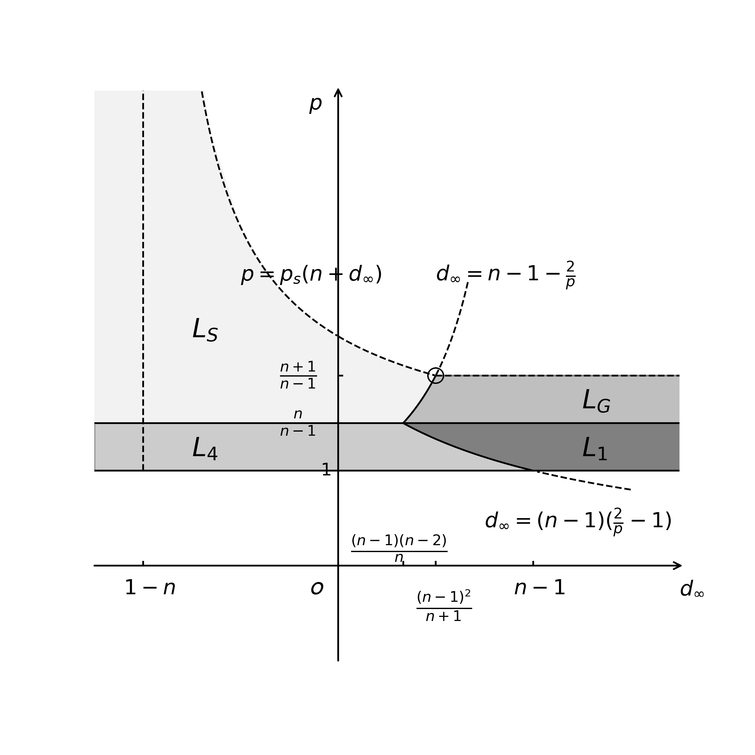
See Figure 1 for the region of $(d_{\infty},p)$ where we have blow up results. Here $L_{j}$ ( $j=1,2,\cdots,6$ ) denote the $j$ -th lifespan, with $L_{S}=L_{6}$ and $L_{G}=L_{3}$ .

Refer to caption — Figure 1. Theorem 1.3: critical powers and lifespan estimates

As mentioned above, when $D=0$ , Yordanov-Zhang [38] has shown blow-up result for $1<p<p_{S}(n)$ and $n\geq 3$ . The restriction for $n\geq 3$ comes from the proof of the existence and asymptotic behavior of test functions. By using ODE and elliptic theory, we could include the case $n=2$ , in the case of the radial nontrivial potential.

Moreover, when $d_{\infty}\leq 1-n$ , we have $p_{S}(n+d_{\infty})=\infty$ and so there are no global solutions for any $p\in(1,\infty)$ . A specific example could be $D=\frac{d_{\infty}}{d_{\infty}+r}$ and $V=V_{\infty}(1+r)^{-2}$ .

Remark 1.4.

Through scaling, we see that the technical condition $1+D(r)+V(r)\geq 0$ could be replaced by the slightly general condition $\lambda_{0}^{2}+\lambda_{0}D(r)+V(r)\geq 0$ for some $\lambda_{0}>0$ .

(III) Critical damping and potential $D=\mathcal{O}(|x|^{-1})$ , $V=\mathcal{O}(|x|^{-2})$ near spatial infinity

Finally, when both the damping and potential terms exhibit certain critical nature, it turns out that we have the blow-up phenomenon under the shifted Strauss exponent and a shifted Glassey exponent, shifted by $\rho(v_{\infty})$ or $d_{\infty}$ .

In [4], Georgiev, Kubo and Wakasa showed that the critical power for the radial solutions is the shifted Strauss exponent $p=p_{S}(3+2)$ , for a special case in $\mathbb{R}^{3}$ , with damping and potential coefficients satisfying the relation

V(r)=-D^{\prime}(r)/2+D^{2}(r)/4,

where $D(r)$ is a positive decreasing function in $C([0,\infty))\cap C^{1}(0,\infty)$ satisfying $D(r)=2/r$ for $r\geq r_{0}>0$ .

In the case of the problem with sample scale-invariant “critical” damping and potential,

D(x)=\frac{d_{\infty}}{|x|},V(x)=\frac{v_{\infty}}{|x|^{2}}\ ,

with $0\leq d_{\infty}<n-1+2\rho(v_{\infty})$ , $v_{\infty}>-(n-2)^{2}/4$ , thanks to the specific structure of the damping and potential terms, Dai, Kubo and Sobajima [2] were able to construct explicit test functions by using hypergeometric functions and obtain the upper bound of the lifespan for

\frac{n+\rho(v_{\infty})}{n+\rho(v_{\infty})-1}<p\leq p_{c}\ .

See also Ikeda-Sobajima [9] for the prior blow-up results for $\frac{n}{n-1}<p\leq p_{S}(n+d_{\infty})$ , when $v_{\infty}=0$ , $n\geq 3$ and $0\leq d_{\infty}<(n-1)^{2}/(n+1)$ .

As we can see, the above results heavily depends on the specific structure of the damping and potential terms. Our next theorem addresses on the problem with a general class of damping and potential terms, which exhibit certain critical nature.

Theorem 1.5.

Consider (1.1) with $n\geq 2$ . Assume that the coefficients $V(x),~{}D(x)$ satisfy:

1. $V(r),D(r)\in C(\mathbb{R}_{+})$ , $V(r)\geq 0$ , $D+V\geq-1$ ;

2. For the part near spatial infinity, $r>1$ ,

$\displaystyle r^{2}V(r)=v_{\infty}+rV_{\infty}(r)$ , $V_{\infty}(r)\in L^{1}_{r>1}$ , $v_{\infty}\geq 0$ (with $v_{\infty}>0$ for $n=2$ );

$\displaystyle rD(r)=d_{\infty}+rD_{\infty}(r),\ D_{\infty}(r)\in L^{1}_{r>1},\ rD_{\infty}\in L^{\infty}_{r>1}$ with $d_{\infty}\in\mathbb{R}$ ;

3. For $r\in(0,1]$ , $D=\mathcal{O}(r^{\theta-2})$ for some $\theta\in[0,2]$ , and

$\displaystyle r^{2}V(r)=v_{0}+rV_{0}(r),\ V_{0}(r)\in L^{1}_{loc}$ for $n\geq 3$ or $v_{0}>0$ ;

$\displaystyle r^{2}D(r)=d_{0}+rD_{0}(r),\ D_{0}(r)\in L_{loc}^{1}$ for $n\geq 3$ or $v_{0}+d_{0}>0$ .
For $n=2$ and the endpoint case, instead of the assumption 3, we assume the analytic conditions for some $\delta>0$ :

3’. $\displaystyle r^{2}V(r)=\sum_{j\geq 1}b_{j}r^{j}$ for $r\in(0,\delta)$ if $v_{0}=0$ ;

$\displaystyle r^{2}(V+D)=\sum_{j\geq 1}c_{j}r^{j}$ for $r\in(0,\delta)$ if $v_{0}+d_{0}=0$ .

Suppose that

p_{0}:=\frac{n+\rho(v_{0})}{n+\rho(v_{0}+\min(0,d_{0}))+\theta-2}<p_{c}=\max(p_{S}(n+d_{\infty}),p_{G}(n+\rho(v_{\infty})),

then for any $p_{0}<p<p_{c}$ , any energy solutions $u$ for (1.1), with $f=0$ , nontrivial, nonnegative and compactly supported $g$ , will blow up in finite time. Moreover, there exist constants $C,\varepsilon_{0}>0$ such that $T_{\varepsilon}$ has to satisfy

(1.13)

T_{\varepsilon}\leq\left\{\begin{array}[]{ll}C\varepsilon^{-(p-1)}&\mbox{if}\ p\in(p_{2},p_{3})\neq\emptyset\\ C\varepsilon^{-(p-1)}\left(\ln\varepsilon^{-1}\right)^{p-1}&\mbox{if}\ p=p_{3}>p_{2}\\ C\varepsilon^{-\frac{p-1}{n+\rho(v_{\infty})+1-(n+\rho(v_{\infty})-1)p}}&\mbox{if}\ p\in(\max(p_{2},p_{3}),p_{G}(n+\rho(v_{\infty})))\neq\emptyset\\ C\varepsilon^{-\frac{2p(p-1)}{\gamma_{2}(p)}}&\mbox{if}\ p\in(p_{0},\min(p_{3},p_{5}))\neq\emptyset\\ C\varepsilon^{-\frac{2p(p-1)}{\gamma(p,n+{d_{\infty}})}}(\ln\varepsilon^{-1})^{\frac{2(p-1)}{\gamma(p,n+{d_{\infty}})}}&\mbox{if}\ p=p_{3}\in(p_{0},p_{S}(n+{d_{\infty}}))\neq\emptyset\\ C\varepsilon^{-\frac{2p(p-1)}{\gamma(p,n+{d_{\infty}})}}&\mbox{if}\ p\in(\max(p_{0},p_{3}),p_{S}(n+{d_{\infty}}))\neq\emptyset\\ C\varepsilon^{-\frac{2(p-1)}{(n+d_{\infty}+1)-(n+d_{\infty}-1)p}}&\mbox{if}\ p\in(p_{4},p_{0}]\cap(p_{4},p_{G}(n+d_{\infty}))\neq\emptyset\end{array}\right.

for $0<\varepsilon\leq\varepsilon_{0}$ . Here $p_{i}$ are defined as follows:

p_{0}=\max(p_{1},p_{2}),\ p_{1}:=\frac{n+\rho(v_{0})}{n+\rho(v_{0}+d_{0})+\theta-2},\ p_{2}:=\frac{n+\rho(v_{0})}{n+\rho(v_{0})+\theta-2}

p_{3}:=\frac{n+\rho(v_{\infty})}{n+\rho(v_{\infty})-1}\ ,\ p_{4}:=\frac{n+\rho(v_{0}+d_{0})}{n+\rho(v_{0}+d_{0})+\theta-2}.

p_{5}=\left\{\begin{array}[]{ll}\frac{3n+d_{\infty}+2\rho(v_{\infty})-1+\sqrt{(3n+d_{\infty}+2\rho(v_{\infty})-1)^{2}-8(n+d_{\infty}-1)(n+\rho(v_{\infty})-1)}}{2(n+d_{\infty}-1)}&n+d_{\infty}>1\\ \infty&n+d_{\infty}\leq 1\ ,\end{array}\right.

and

(1.14)

\gamma_{2}(p):=2(n+\rho(v_{\infty})-1)(p-p_{3})+\gamma(p,n+d_{\infty})\ ,

where $\gamma$ is given in (1.7) and $p_{5}$ is the positive root of $\gamma_{2}(p)=0$ when $n+d_{\infty}>1$ .

Remark 1.6.

We observe that, in our statement, besides the expected upper bound of the blow up range, we have certain lower bound, which depends on the local behavior of $V(x)$ and $D(x)$ near the origin, as well as $v_{\infty}$ for $p_{3}$ . Heuristically, we expect that the lower bounds for the blow-up range are just technical conditions. In other words, we conjecture that we still have blow up results for any $p\in(1,p_{c})$ .

Remark 1.7.

When $n=3$ , $v_{0}=d_{0}=0$ , $v_{\infty}=d_{\infty}=2$ , and $\theta=2$ , we have $p_{1}=p_{2}=1$ , $p_{3}=4/3$ , and thus recover the blow-up result in [4] for $1<p<p_{S}(5)$ . When $d_{0}=0$ , $d_{\infty}=A$ , $v_{0}=v_{\infty}=B$ and $\theta=1$ , our result recovers and generalizes the subcritical results in [2]. The blow-up and lifespan estimate for the “critical” power are lost in our result, which seems to be much more delicate to obtain, in our general setting for the damping and potential functions. One of the unexpected features is that we could obtain blow up results for highly singular damping term near the origin. For example, for any $d_{0},v_{0},d_{\infty},v_{\infty}>0$ such that $p_{0}<p_{c}$ , the problem with

D=\frac{d_{0}}{r^{2}}+\frac{d_{\infty}}{r},\ V=\frac{v_{0}}{r^{2}}+\frac{2(v_{\infty}-v_{0})\arctan r}{\pi r^{2}}\ ,

could not admit global solutions in general, for $p\in(p_{0},p_{c})$ , despite the strong damping effect near the origin.

Concerning the comparison of the exponents $p_{i}$ , $p_{S}$ and $p_{G}$ , they depend on the the damping, potential and dimension. For example, we observe from (1.14) and (1.7) for $\gamma_{2}$ and $\gamma(p,n)$ , whose positive roots give $p_{5}$ and $p_{S}$ , as well as the obvious relation $p_{3}<p_{G}(n+\rho(v_{\infty}))$ , that we always have

\min(p_{3},p_{5})<p_{c}\ .

As $n+\rho(d_{\infty})-1>0$ , we have $\gamma_{2}(p)<\gamma(p,n+d_{\infty})$ for $p<p_{3}$ , which shows that the current lifespan estimate for $p_{0}<p<\min(p_{3},p_{5})$ is weaker than the standard one. Also, it is clear that $p_{1}<p_{2}$ iff $d_{0}>0,\theta<2$ , which is also equivalent to $p_{4}<p_{2}$ .

In relation with Remark 1.6, we would like to show blow up results for any $p\in(1,p_{c})$ . It is clear that when $\theta=2$ (which ensures that $d_{0}=0$ ), we have $p_{0}=1$ and so is the blow up results for $p\in(1,p_{c})$ . Moreover, by examining the proof of Theorem 1.5, in particular the estimates (4.8) and (4.3), we find that the technical condition $p_{3}$ for the lifespan estimates could also be avoided if the damping term vanishes $D=0$ near spatial infinity. That is, when $D(r)\in C_{c}([0,\infty))$ (so that $d_{0}=d_{\infty}=0$ and $\theta=2$ ), we have

F_{0}=\int_{T/2}^{T}\int_{B_{t+R}}T^{-2p^{\prime}}\phi_{0}dxdt{\lesssim}T^{-2p^{\prime}+\rho(v_{\infty})+n+1}\ ,

and so is the following

Corollary 1.8.

Under the same assumptions as in Theorem 1.5, with an additional assumption that $D(|x|)\in C_{c}([0,\infty))$ . Then we have blow up results for any $1<p<p_{c}=\max(p_{G}(n+\rho(v_{\infty})),p_{S}(n))$ . In addition, we have, for some constants $C,\varepsilon_{0}>0$ ,

(1.15)

T_{\varepsilon}\leq\left\{\begin{array}[]{ll}L_{S}=C\varepsilon^{-\frac{2p(p-1)}{\gamma(p,n)}}&\mbox{if}\ p\in(1,p_{S}(n))\\ L_{G}=C\varepsilon^{-\frac{p-1}{n+\rho(v_{\infty})+1-(n+\rho(v_{\infty})-1)p}}&\mbox{if}\ p\in(1,p_{G}(n+\rho(v_{\infty})))\end{array}\right.

for any $0<\varepsilon\leq\varepsilon_{0}$ .

See Figure 2 for the region of $(v_{\infty},p)$ where we have blow up results for $n=2$ . As we assume $v_{\infty}\geq 0$ , we always have $p_{S}(n)>p_{G}(n+\rho(v_{\infty}))$ and the second upper bound $L_{G}$ is effective (i.e., $L_{G}\leq L_{S}$ for $\varepsilon\ll 1$ if and only if $(2\rho(v_{\infty})+n-1)p\leq 2$ , which is nonempty only if $n\leq 2$ .

Figure 2. Corollary 1.8: lifespan estimates for

n=2

For the strategy of proof, we basically follow the test function method. The key ingredient is to construct special positive standing wave solutions, of the form $w=e^{-\lambda t}\phi_{\lambda}(x)$ , to the linear dual problem,

(\partial_{t}^{2}-\Delta-D\partial_{t}+V)w=0\ ,

with the desired asymptotic behavior. In turn, it is reduced to constructing solutions to certain elliptic “eigenvalue” problems:

(1.16)

(\lambda^{2}-\Delta+D\lambda+V)\phi_{\lambda}=0\ .

Concerning the subcritical blow up results, $p<p_{c}$ , it suffices to construct solutions for (1.16) with $\lambda=0$ and some $\lambda_{0}>0$ . While for the critical case, we will also need to find solutions with uniform estimates with respect to all $\lambda\in(0,\lambda_{0})$ .

Outline

Our paper is organized as follows. In Section 2, we present the existence results of special solutions for the elliptic “eigenvalue” problems (1.16), with certain asymptotic behavior, by applying elliptic and ODE theory. These solutions play a key role in constructing the test functions and the proof of blow up results. The proof of the existence results are given in Section 3. Equipped with the eigenfunctions, the test function method is implemented in Section 4, to give the proof of Theorem 1.5. Then, in Section 5, we give the proof of Theorem 1.3, when $n\geq 2$ and the potential is of short range. In essence, with the help of Lemma 2.2 and 2.4, Theorem 1.3 could be viewed as a corollary of Theorem 1.5 when $n\geq 3$ . At last, in Section 6, we present the required test function for the critical case, as well as the upper bound and lower bound estimates. Equipped with the test function, a relatively routine argument (see, e.g., [18] or [17]) will yield Theorem 1.2.

Notations.

We close this section by listing the notation. Let $\langle x\rangle=\sqrt{1+|x|^{2}}$ for $x\in\mathbb{R}^{n}$ . We will also use $A{\lesssim}B$ to stand for $A\leq CB$ where the constant $C$ may change from line to line.

2. Solutions to elliptic equations

In this section, we present the existence results of special solutions for some elliptic “eigenvalue” problems, with certain asymptotic behavior, which would be used to construct test functions to derive the expected lifespan estimates. We will consider two types of elliptic equations.

2.1. Eigenfunction for $V-\Delta$

At first, we consider the “zero-eigenfunction” for the positive elliptic operator $V-\Delta$ .

Lemma 2.1.

Suppose $0\leq V\in C(\mathbb{R}^{n}\backslash\{0\})$ and

r^{2}V(r)=v_{\infty}+rV_{\infty}(r)=v_{0}+rV_{0}(r)\ ,V_{\infty}(r)\in L^{1}_{r>1}\ ,V_{0}(r)\in L^{1}_{r<1}\ ,

Then if $n\geq 3$ or $v_{0},v_{\infty}>0$ , there exists a solution $\phi_{0}\in H_{loc}^{1}(\mathbb{R}^{n})\cap W_{loc}^{2,1+}(\mathbb{R}^{n})$ of

(2.1)

\Delta\phi_{0}=V\phi_{0},\ x\in\mathbb{R}^{n},\ \ n\geq 2,\

satisfying

(2.2)

\begin{split}\phi_{0}\simeq\begin{cases}r^{\rho(v_{0})},\ r\leq 1,\\ r^{\rho(v_{\infty})},\ r\geq 1\ .\end{cases}\end{split}

In addition, for $n=2$ with $v_{0}=0$ , if we assume $r^{2}V$ is analytic in $(0,\delta)$ for some $\delta>0$ , i.e.,

r^{2}V(r)=\sum^{\infty}_{j=1}b_{j}r^{j},\ 0<r<\delta\ ,

then the same result holds.

When $V$ is Hölder continuous near the origin, the regularity of the solutions could be improved.

Lemma 2.2.

Suppose $0\leq V\in C(\mathbb{R}^{n})$ , $V=V(r)=\mathcal{O}(\langle r\rangle^{-\beta})$ for some $\beta>2$ , and $V\in C^{\delta}(B_{\delta})$ for some $\delta>0$ . In addition, we assume $V$ is nontrivial when $n=2$ . Then there exists a $C^{2}$ solution of (2.1) satisfying

(2.3)

\begin{split}\phi_{0}\simeq\begin{cases}\ln(r+2),\ n=2,\\ 1,\ \ n\geq 3.\ \end{cases}\end{split}

Moreover, when $n=2$ and $V\equiv 0$ , it is clear that $\phi_{0}=1$ is a solution (2.1).

When $n\geq 3$ , $V$ is locally Hölder continuous (not necessarily radial) and $0\leq V\leq\frac{C}{1+|x|^{2+\delta}}$ with $C,\delta>0$ , Lemma 2.2 was known from Yordanov-Zhang [38].

2.2. “Eigenfunction” for $V+D-\Delta$ with negative “eigenvalue”

In this subsection, we consider the “eigenfunction” for $V+D-\Delta$ with negative “eigenvalue”:

(2.4)

\Delta\phi_{\lambda_{0}}=(\lambda_{0}^{2}+\lambda_{0}D+V)\phi_{\lambda_{0}},\ \lambda_{0}>0,\ \ x\in\mathbb{R}^{n}.\

Lemma 2.3.

Let $V=V(r),D=D(r)\in C(0,\infty)$ . Suppose $V\geq 0$ , $D\geq-\lambda_{0}-\frac{V}{\lambda_{0}}$ for some $\lambda_{0}>0$ , and

D(r)=\frac{d_{0}}{r^{2}}+\frac{1}{r}D_{0}(r),\ V(r)=\frac{v_{0}}{r^{2}}+\frac{1}{r}V_{0}(r),\ r\leq 1,\

with $D_{0}(r)\in L^{1}_{r<1}$ , $V_{0}(r)\in L^{1}_{r<1}$ . In addition, we assume for some $d_{\infty}\in\mathbb{R}$ ,

V(r)\in L^{1}_{r>1},\ D(r)=\frac{d_{\infty}}{r}+D_{\infty}(r),\ D_{\infty}(r)\in L^{1}_{r>1}.\

Then if $n\geq 3$ or $v_{0}+\lambda_{0}d_{0}>0$ , there exists a $H_{loc}^{1}(\mathbb{R}^{n})\cap W_{loc}^{2,1+}(\mathbb{R}^{n})$ solution of (2.4) satisfying

(2.5)

\begin{split}\phi_{\lambda_{0}}\sim\begin{cases}r^{\rho(v_{0}+\lambda_{0}d_{0})},\ r\leq 1,\\ r^{-\frac{n-1-d_{\infty}}{2}}e^{\lambda_{0}r},\ r\geq 1.\end{cases}\end{split}

In addition, we have the same result for $n=2$ with $v_{0}+\lambda_{0}d_{0}=0$ , when $r^{2}(V+\lambda_{0}D)$ is analytic near $0$ :

r^{2}(V+\lambda_{0}D)=\sum^{\infty}_{j=1}c_{j}r^{j}\ ,0<r<\delta\ .

Lemma 2.4.

Let $V=V(r),D=D(r)\in C(\mathbb{R}^{n})\cap C^{\delta}(B_{\delta})$ for some $\delta>0$ . Suppose $V\geq 0$ , $D\geq-\lambda_{0}-\frac{V}{\lambda_{0}}$ , and also that for some $d_{\infty}\in\mathbb{R}$ , $R>1$ and $r\geq R$ , we have

V(r)\in L^{1}([R,\infty))\ ,\ D(r)=\frac{d_{\infty}}{r}+D_{\infty}(r),\ D_{\infty}(r)\in L^{1}([R,\infty))\ .

Then there exists a $C^{2}$ solution of (2.4) satisfying

(2.6)

\phi_{\lambda_{0}}\simeq\langle r\rangle^{-\frac{n-1-d_{\infty}}{2}}e^{\lambda_{0}r}\ .

2.3. Eigenvalue problem with parameters

To handle the critical problem, we will need to construct a class of (unbounded) positive solutions for the eigenvalue problem, with certain uniform estimates for small parameters.

Lemma 2.5.

Let $n\geq 2$ , $\beta>1$ , $\mu\geq 0$ . Suppose $D(x)\in C(\mathbb{R}^{n})\cap C^{\delta}(B_{\delta})$ for some $\delta>0$ and $0\leq D(x)\leq\frac{\mu}{(1+|x|)^{\beta}}$ . Then there exists $c_{1}\in(0,1)$ such that for any $0<\lambda\leq 1$ , there is a $C^{2}$ solution of

(2.7)

\Delta\phi_{\lambda}-\lambda D(x)\phi_{\lambda}=\lambda^{2}\phi_{\lambda}

satisfying

(2.8)

c_{1}\langle\lambda|x|\rangle^{-\frac{n-1}{2}}e^{\lambda|x|}<\phi_{\lambda}(x)<c_{1}^{-1}\langle\lambda|x|\rangle^{-\frac{n-1}{2}}e^{\lambda|x|}\ .

3. Proof of Lemmas 2.1-2.5

In this section, we present the proof of Lemmas 2.1-2.5. by applying elliptic and ODE theory.

3.1. Proof of Lemma 2.1

We will find a radial solution $\phi_{0}(x)=\phi_{0}(|x|)=\phi_{0}(r)$ .

At first, for the region $0<r\leq 1$ , we observe that the equation in $r$ is of the Euler type:

\Delta\phi_{0}=(\partial^{2}_{r}+\frac{n-1}{r}\partial_{r})\phi_{0}=V\phi_{0}\ ,

for which it is natural to introduce a new variable $t$ with $r=e^{-t}$ . Then $f(t)=\phi_{0}(e^{-t})$ satisfies

\partial^{2}_{t}f-(n-2)\partial_{t}f=(v_{0}+e^{-t}V_{0}(e^{-t}))f\ ,t\geq 0\ .

Let $Y(t)=(Y_{1}(t),Y_{2}(t))^{T}$ with $Y_{1}=f$ , $Y_{2}=\partial_{t}f$ , then we have

Y^{\prime}=(A+B(t))Y,A=\left(\begin{array}[]{cc}0&1\\ v_{0}&n-2\end{array}\right),B(t)=\left(\begin{array}[]{cc}0&0\\ e^{-t}V_{0}(e^{-t})&0\end{array}\right)\ .

As $V_{0}(r)\in L^{1}_{r<1}$ , that is, $B\in L^{1}[0,\infty)$ , we could apply the Levinson theorem (see, e.g., [1, Chapter 3, Theorem 8.1]) to the system. Then there exists $t_{0}\in[0,\infty)$ so that we have two independent solutions, which have the asymptotic form as $t\to\infty$

Y_{+}(t)=\left(\begin{array}[]{c}1+o(1)\\ \lambda_{1}+o(1)\end{array}\right)e^{\lambda_{1}t}\ ,\ Y_{-}(t)=\left(\begin{array}[]{c}1+o(1)\\ \lambda_{2}+o(1)\end{array}\right)e^{\lambda_{2}t}\ ,

where $\lambda_{1}=\sqrt{(\frac{n-2}{2})^{2}+v_{0}}+\frac{n-2}{2}$ , $\lambda_{2}=-\sqrt{(\frac{n-2}{2})^{2}+v_{0}}+\frac{n-2}{2}=-\rho(v_{0})$ .

We choose $Y(t)=Y_{-}(t)$ so that

\phi_{0}(r)=f(-\ln r)=(1+o(1))r^{\rho(v_{0})}

as $r\to 0$ . It is easy to check that $\phi_{0}\in H^{1}(B_{\delta})\cap W^{2,1+}(B_{\delta})$ , and

\partial_{r}\phi_{0}=-r^{-1}\partial_{t}f|_{t=-\ln r}=(\rho(v_{0})+o(1))r^{\rho(v_{0})-1}

for $r\in(0,1]$ . Based on the assumption $n\geq 3$ or $v_{0}>0$ , we have $\rho(v_{0})>0$ and so there exists $\delta_{0}>0$ such that

(3.1)

\partial_{r}\phi_{0}\simeq r^{\rho(v_{0})-1}\ ,r\in(0,\delta_{0})\ .

In addition, for the case $n=2$ and $v_{0}=0$ when $r^{2}V$ is analytic in $(0,\delta)$ , by applying the Frobenius method, there is an analytic solution

\phi_{0}=r^{\lambda_{1}}\sum^{+\infty}_{j=0}a_{j}r^{j}\sim 1,\ r<\delta\ ,

with $a_{0}=1$ , where $\lambda_{1}=\rho(v_{0})=0$ is the root of $\lambda^{2}=0$ . If $V\equiv 0$ near $0$ , then $\phi_{0}=1$ . Otherwise, there exists $k>0$ such that $b_{j}=0$ for all $j<k$ and $b_{k}>0$ , in which we have $a_{j}=b_{j}/j^{2}$ for any $j\in[1,k]$ . Thus once again we have, for some $\delta_{0}>0$ ,

\partial_{r}\phi_{0}\simeq(\frac{b_{k}}{k}+o(1))r^{k-1}\ ,r\in(0,\delta_{0})\ .

Similarly, for $r>1$ , let $r=e^{t}$ , then $F(t)=\phi_{0}(e^{t})$ satisfies

\partial^{2}_{t}F+(n-2)\partial_{t}F=(v_{\infty}+e^{t}V_{\infty}(e^{t}))F\ ,t\geq 0\ .

Applying the Levinson theorem again, we know that there exists $c_{1},c_{2}$ such that

\phi_{0}(e^{t})=c_{1}(1+o(1))e^{\rho(v_{\infty})t}+c_{2}(1+o(1))e^{(-\rho(v_{\infty})-(n-2))t},

\partial_{t}\phi_{0}(e^{t})=c_{1}(\rho(v_{\infty})+o(1))e^{\rho(v_{\infty})t}+c_{2}(2-n-\rho(v_{\infty})+o(1))e^{(-\rho(v_{\infty})-(n-2))t}

as $t\to\infty$ . Notice that $\rho(v_{\infty})>0$ , due to the assumption $n\geq 3$ or $v_{\infty}>0$ .

By the fundamental well-posed theory of linear ordinary differential equation, we know that $\phi_{0}(r)\in C^{2}(0,\infty)$ . We claim that $\partial_{r}\phi_{0}(r)\geq 0$ for all $r>0$ . Actually, we have seen from (3.1) that $\phi_{0}>0$ and $\partial_{r}\phi_{0}\geq 0$ for $r\in(0,\delta_{0})$ . Suppose, by contradiction, there exists a $r_{2}>\delta_{0}$ such that $\phi^{\prime}_{0}(r_{2})<0$ with $\phi_{0}(r)\geq 0$ for any $r\in(0,r_{2}]$ . Then there is a $r_{1}<r_{2}$ such that $\partial_{r}\phi_{0}(r_{1})=0$ . Recall that

\partial_{r}(r^{n-1}\partial_{r}\phi_{0})=r^{n-1}V\phi_{0}\ .

By integrating it form $r_{1}$ to $r_{2}$ , we get

r^{n-1}_{2}\phi^{\prime}_{0}(r_{2})=\int^{r_{2}}_{r_{1}}\tau^{n-1}V\phi_{0}(\tau)d\tau\geq 0\ ,

which is a contradiction. Hence we get $c_{1}>0$ and

\phi_{0}\sim r^{\rho(v_{\infty})},\partial_{r}\phi_{0}\sim r^{\rho(v_{\infty})-1}\ r\gg 1\ .

3.2. Proof of Lemma 2.2

Suppose $V$ is Hölder continuous in $\overline{B_{\delta}}$ for some $\delta>0$ . Then we consider the Dirichlet problem

(3.2)

\begin{cases}\Delta\phi_{0}=V\phi_{0},x\in B_{\delta}\\ \phi_{0}|_{\partial B_{\delta}}=1\end{cases}

By Gilbarg-Trudinger [6, Theorem 6.14], there exists a unique $C^{2}(\overline{B_{\delta}})$ solution, which must be radial. For $r>0$ , with $\phi_{0}(x)=\phi_{0}(r)$ , (3.2) becomes an ordinary differential equation

(3.3)

\begin{cases}\phi^{\prime\prime}_{0}+\frac{n-1}{r}\phi^{\prime}_{0}-V\phi_{0}=0\\ \phi_{0}(\delta)=1,\phi^{\prime}_{0}(\delta)=C\end{cases}

Then by the theory of ordinary differential equation, there is a unique solution $\phi_{0}(r)\in C^{2}(0,\infty)$ , which agrees with $\phi_{0}$ in $B_{\delta}$ . Thus we get a solution $\phi_{0}(x)\in C^{2}(\mathbb{R}^{n})$ and we could apply strong maximum principle to get $\partial_{r}\phi_{0}\geq 0$ for all $r>0$ and $\phi_{0}(0)>0$ .

Recall that

(3.4)

\partial_{r}(r^{n-1}\partial_{r}\phi_{0})=r^{n-1}V\phi_{0}\ .

By integrating it from $0$ to $r$ , we get

(3.5)

r^{n-1}\partial_{r}\phi_{0}=\int^{r}_{0}\tau^{n-1}V\phi_{0}d\tau\ {\lesssim}\ \phi_{0}\int^{r}_{0}(1+\tau)^{n-1-\beta}d\tau\ .

Thus, as $\beta>2$ , if $n\geq 3$ and $r\geq 1$ , we have

\partial_{r}\phi_{0}\ {\lesssim}\ \phi_{0}r^{1-n}\int^{r}_{0}(1+\tau)^{n-1-\beta}d\tau{\lesssim}\phi_{0}r^{-1-\delta}\ ,

for some $\delta>0$ . By Gronwall’s inequality, we obtain $\phi_{0}{\lesssim}\phi_{0}(1)$ , for all $r\geq 1$ , which yields

\phi_{0}\simeq 1\ .

For $n=2$ , since $V$ is nontrivial, then there exists some $R>0$ such that $V\neq 0$ when $R\leq r\leq 2R$ . By (3.4), we have

r\partial_{r}\phi_{0}=R\partial_{r}\phi_{0}(R)+\int^{r}_{R}\tau V\phi_{0}d\tau\ \geq\ \phi_{0}(R)R\int^{2R}_{R}V(\tau)d\tau\geq C\ ,\ r\geq 2R\ ,

hence we get

\phi_{0}(r)\geq\phi_{0}(R)+\int^{r}_{R}\frac{C}{\tau}d\tau\geq C\ln\frac{r}{R}+\phi_{0}(R)\ {\gtrsim}\ \ln(2+r),\ r\geq 2R\ .

On the other hand, by (3.5), we have

r\partial_{r}\phi_{0}=\int^{r}_{0}\tau V\phi_{0}d\tau\ {\lesssim}\ \phi_{0}(r)\int^{\infty}_{0}(1+\tau)^{1-\beta}d\tau\ {\lesssim}\ \phi_{0}(r)\ ,

which gives us

(3.6)

\phi_{0}\ {\lesssim}\ 1+r\ ,\forall\ r\geq 0\ .

By inserting (3.6) into (3.5), we have for any $\delta_{1}\in(0,\beta/2-1)$ and $r\geq 1$

(3.7)

\partial_{r}\phi_{0}{\lesssim}\left\{\begin{array}[]{ll}r^{-1},&\beta>3,\\ r^{2-\beta+\delta_{1}},&\ 2<\beta\leq 3\ .\end{array}\right.

Then it easy to obtain the desired upper bound $\ln(2+r)$ for $\beta>3$ , while for $\beta\leq 3$ , we get $\phi_{0}(r){\lesssim}(1+r)^{3-\beta+\delta_{1}}$ for any $r\geq 0$ which is better than (3.6).

Thus, to obtain the expected upper bound, we do the iteration, by inserting the improved upper bound $\phi_{0}(r){\lesssim}(1+r)^{3-\beta+\delta_{1}}=(1+r)^{k}$ into (3.5) to get, for $r>1$ ,

\partial_{r}\phi_{0}{\lesssim}\begin{cases}r^{-1},\ k+2<\beta\\ r^{k+1-\beta+\delta_{2}},\ k+2\geq\beta,\end{cases}\phi_{0}{\lesssim}\begin{cases}\ln(2+r),\ k+2<\beta\\ (1+r)^{k+2-\beta+\delta_{2}},\ k+2\geq\beta\ ,\end{cases}

for any $\delta_{2}\in(0,\beta/2-1)$ . For $k+2\geq\beta$ , we can get the improved upper bound. By repeating (finitely) steps, we can finally obtain

\phi_{0}(r){\lesssim}\ln(2+r)\ ,\forall\ r\geq 0\ .

3.3. Proof of Lemma 2.3

To start with, we record a lemma from Liu-Wang [23] which we will use later.

Lemma 3.1 (Lemma 3.1 in [23]).

Let $\lambda\in(0,\lambda_{0}]$ , $\delta_{0}\in(0,1)$ , $\epsilon>0$ , $y_{0}>0$ , $K\in(\delta_{0},\delta_{0}^{-1})$ ,

(3.8)

\|K^{\prime}\|_{L^{1}([\epsilon\lambda_{0}^{-1},\infty))}\leq\delta_{0}^{-1},\|G\|_{L^{1}([\epsilon\lambda^{-1},\infty))}\leq\delta_{0}^{-1}\lambda,\forall\lambda\in(0,\lambda_{0}]\ .

Considering

(3.9)

\begin{cases}y^{\prime\prime}-\lambda^{2}K^{2}(r)y+G(r)y=0,r>\epsilon\lambda^{-1}\\ y(\epsilon\lambda^{-1})=y_{0},y^{\prime}(\epsilon\lambda^{-1})=y_{1}\in(0,\delta_{0}^{-1}\lambda y_{0})\end{cases}

Then for any solution $y$ with $y,y^{\prime}>0$ , we have the following uniform estimates, independent of $\lambda\in(0,\lambda_{0}]$ ,

(3.10)

y\simeq y_{0}e^{\lambda\int^{r}_{\epsilon/\lambda}K(\tau)d\tau}\ ,\ r\geq\epsilon\lambda^{-1}\ .

Assume in addition $1-\lambda^{-2}K^{-2}G\in(\delta_{0},\delta_{0}^{-1})$ , then the solution $y$ to (3.9) satisfies $y,y^{\prime}>0$ and we have

(3.11)

y^{\prime}\simeq y_{1}+y_{0}\lambda(e^{\lambda\int^{r}_{\epsilon/\lambda}K(\tau)d\tau}-1)\ .

Proof of Lemma 2.3.

For $r\leq\delta$ , by the similar proof of Lemma 2.1, there is a solution $\phi_{\lambda_{0}}$ satisfying

\phi_{\lambda_{0}}\sim r^{\rho(v_{0}+\lambda_{0}d_{0})}\ ,\phi_{\lambda_{0}}\in H^{1}(B_{\delta})\cap W^{2,1+}(B_{\delta}),\partial_{r}\phi_{\lambda_{0}}\geq 0\ .

When $r\geq\delta$ , with $\phi_{\lambda_{0}}(x)=\phi_{\lambda_{0}}(r)$ , we need only to consider the following ordinary differential equation

(3.12)

\phi^{\prime\prime}_{\lambda_{0}}+\frac{n-1}{r}\phi^{\prime}_{\lambda_{0}}=(\lambda_{0}^{2}+\lambda_{0}D+V)\phi_{\lambda_{0}}\ ,\phi_{\lambda_{0}}(\delta)=C_{1}>0,\ \partial_{r}\phi_{\lambda_{0}}(\delta)=C_{2}\geq 0\ .

Then, as in the proof of Lemma 2.1, there is a unique solution $\phi_{\lambda_{0}}(r)\in C^{2}(0,\infty)$ and $\partial_{r}\phi_{\lambda_{0}}(r)\geq 0$ for all $r>0$ .

For $r\geq R$ , we shall consider (3.12) with $\phi_{\lambda_{0}}(R)>0$ and $\phi^{\prime}_{\lambda_{0}}(R)\geq 0$ . Let $y=r^{\frac{n-1}{2}}\phi_{\lambda_{0}}$ , then the new function $y$ satisfies

(3.13)

\begin{cases}y^{\prime\prime}-(\lambda_{0}^{2}+\frac{d_{\infty}}{r}\lambda_{0})y-(\frac{(n-1)(n-3)}{4r^{2}}+V+\lambda_{0}D_{\infty})y=0\\ y(R)=R^{\frac{n-1}{2}}\phi_{\lambda_{0}}(R),y^{\prime}(R)\geq\frac{n-1}{2}R^{\frac{n-3}{2}}\phi_{\lambda_{0}}(R)>0\end{cases}

Thus by Lemma 3.1, we have

y\simeq e^{\int^{r}_{R}(\sqrt{\lambda_{0}^{2}+\lambda_{0}\frac{d_{\infty}}{\tau}})d\tau}\simeq r^{\frac{d_{\infty}}{2}}e^{\lambda_{0}r},r\geq R\ ,

which yields

\phi_{\lambda_{0}}\simeq r^{-\frac{n-1-d_{\infty}}{2}}e^{\lambda_{0}r},r\geq R\ .

∎

3.4. Proof of Lemma 2.4

Suppose $\lambda_{0}^{2}+V+\lambda_{0}D$ is Hölder continuous in $\overline{B_{\delta}}$ for some $\delta>0$ . Then we consider the Dirichlet problem

(3.14)

\begin{cases}\Delta\phi_{\lambda_{0}}=(\lambda_{0}^{2}+\lambda_{0}D+V)\phi_{\lambda_{0}},x\in B_{\delta}\\ \phi_{\lambda_{0}}|_{\partial B_{\delta}}=1.\end{cases}

By Theorem 6.14 in Gilbarg-Trudinger [6], there exists a unique $C^{2}(\overline{B_{\delta}})$ solution. Hence we could apply maximum principle to get $0<\phi_{\lambda_{0}}\leq 1$ in $B_{\delta}$ and $\partial_{r}\phi_{\lambda_{0}}\geq 0$ for all $0<r\leq\delta$ . When $r\geq\delta$ , with $\phi_{\lambda_{0}}(x)=\phi_{\lambda_{0}}(r)$ , (3.14) becomes an ordinary differential equation

(3.15)

\begin{cases}\phi^{\prime\prime}_{\lambda_{0}}+\frac{n-1}{r}\phi^{\prime}_{\lambda_{0}}-(\lambda_{0}^{2}+\lambda_{0}D+V)\phi_{\lambda_{0}}=0\\ \phi_{\lambda_{0}}(\delta)=1,\phi^{\prime}_{\lambda_{0}}(\delta)=C_{2}\geq 0.\end{cases}

Then $\phi_{\lambda_{0}}\in C^{2}(\mathbb{R}^{n})$ and we could apply strong maximum principle again to get $\partial_{r}\phi_{\lambda_{0}}\geq 0$ for all $r>0$ .

Furthermore, for $r\geq R$ , we consider (3.15) from $r=R$ , then we have $\phi_{\lambda_{0}}(R)>0,\phi^{\prime}_{\lambda_{0}}(R)\geq 0$ . By the same argument as in the proof of Lemma 2.3, we get

\phi_{\lambda_{0}}\simeq r^{-\frac{n-1-d_{\infty}}{2}}e^{\lambda_{0}r},r\geq R\ ,

which completes the proof.

3.5. Proof of Lemma 2.5

We first show that (2.7) admits a $C^{2}(\mathbb{R}^{n})$ solution. For $r\leq\lambda^{-1}$ , we consider the Dirichlet problem within $B_{\lambda^{-1}}$

(3.16)

\begin{cases}\Delta\phi_{\lambda}-\lambda D(x)\phi_{\lambda}=\lambda^{2}\phi_{\lambda},x\in B_{\lambda^{-1}}\\ \phi_{\lambda}|_{\partial B_{\lambda^{-1}}}=1\ .\end{cases}

By Theorem 6.14 in Gilbarg-Trudinger [6], there exists a unique (and hence radial) $C^{2}(B_{\lambda^{-1}})$ solution. For $r>0$ , the equation is reduced (2.7) to a second order ordinary differential equation

\phi^{\prime\prime}_{\lambda}+\frac{n-1}{r}\phi^{\prime}_{\lambda}-\lambda D(r)\phi_{\lambda}=\lambda^{2}\phi_{\lambda}\ ,

which ensures that $\phi_{\lambda}\in C^{2}(\mathbb{R}^{n})$ . To obtain (2.8), we need to divide $\mathbb{R}^{n}$ into two parts: $B_{1/\lambda}$ and $\mathbb{R}^{n}\backslash B_{1/\lambda}$ .

(I) Inside the ball $B_{1/\lambda}$

Considering the Dirichlet problem (3.16) within $B_{1/\lambda}$ , it is easy to see that $0<\phi_{\lambda}\leq 1$ in $B_{1/\lambda}$ . In fact, if there exists $x_{0}\in B_{1/\lambda}$ such that $\phi_{\lambda}(x_{0})\leq 0$ , then by strong maximum principle, we get $\phi_{\lambda}$ is constant within $B_{1/\lambda}$ , which is a contradiction. By Hopf’s lemma, we have $\partial_{r}\phi_{\lambda}>0$ for $0<r\leq 1/\lambda$ .

To get the uniform lower bound of $\phi_{\lambda}$ , we define rescaled function $f_{\lambda}(x)=\phi_{\lambda}(x/\lambda)$ , which satisfies

\displaystyle\begin{cases}\Delta f_{\lambda}-\frac{1}{\lambda}D(\frac{r}{\lambda})f_{\lambda}=f_{\lambda},x\in B_{1}\\ f_{\lambda}|_{\partial B_{1}}=1\ .\end{cases}

Since $f_{\lambda}$ is radial increasing, we know that

\liminf_{0<\lambda\leq 1}\inf_{x\in B_{1}}f_{\lambda}=\liminf_{0<\lambda\leq 1}f_{\lambda}(0):=C\geq 0\ .

To complete the proof, we need only to prove $C>0$ . By definition, there exists a sequence $\lambda_{j}\to 0$ such that $f_{\lambda_{j}}(0)\to C$ as $j\to\infty$ .

(i) Derivative estimates of $f_{\lambda}$ .

As $f_{\lambda}$ is radial, we have

\Delta f_{\lambda}=r^{1-n}\partial_{r}(r^{n-1}\partial_{r}f_{\lambda})\ ,

and so

(3.17)

\partial_{r}(r^{n-1}\partial_{r}f_{\lambda})=\Big{(}\frac{1}{\lambda}D(\frac{r}{\lambda})+1\Big{)}r^{n-1}f_{\lambda}.

Recall that $f_{\lambda}\in(0,1]$ and $D(r)\leq\frac{\mu}{(1+|x|)^{\beta}}$ , by integrating it from $0$ to $r$ , we get

	$\displaystyle r^{n-1}\partial_{r}f_{\lambda}=$	$\displaystyle\int_{0}^{r}\Big{(}\frac{1}{\lambda}D(\frac{\tau}{\lambda})+1\Big{)}\tau^{n-1}f_{\lambda}d\tau$
	$\displaystyle\leq$	$\displaystyle\int_{0}^{r}\Big{(}\frac{\mu\lambda^{\beta-1}}{(\lambda+\tau)^{\beta}}+1\Big{)}\tau^{n-1}f_{\lambda}d\tau$
	$\displaystyle\leq$	$\displaystyle\int_{0}^{r}\Big{(}\frac{\mu}{\tau}+1\Big{)}\tau^{n-1}d\tau$
	$\displaystyle\leq$	$\displaystyle\frac{\mu}{n-1}r^{n-1}+\frac{r^{n}}{n}\ ,$

that is,

(3.18)

\partial_{r}f_{\lambda}\leq\frac{\mu}{n-1}+\frac{r}{n}\ .

(ii) Convergence of $f_{\lambda}$ .

Since $\|f_{\lambda}\|_{H^{1}(B_{1})}$ are uniformly bounded, there exists a subsequence of $\lambda_{j}$ (for simplicity we still denote the subsequence as $\lambda_{j}$ ) such that $f_{\lambda_{j}}$ converges weakly to some $f$ in $H^{1}(B_{1})$ as $j$ goes to infinity. Moreover, by the Arzela-Ascoli theorem, $f_{\lambda_{j}}$ converges uniformly to $f$ in $C(\bar{B}_{1})$ as $j$ goes to infinity, thus $f=1$ on $\partial B_{1}$ and $f(0)=C$ .

In view of the equations satisfied by $f_{\lambda_{j}}$ , we see that, for any $\phi\in C^{\infty}_{c}(B_{1})$ , we have

(3.19)

\int_{B_{1}}\nabla f_{\lambda_{j}}\nabla\phi+f_{\lambda_{j}}\phi+\frac{1}{\lambda_{j}}D\big{(}\frac{r}{\lambda_{j}}\big{)}f_{\lambda_{j}}\phi dx=0\ .

Let $g_{\lambda_{j}}=\frac{1}{\lambda_{j}}D(\frac{r}{\lambda_{j}})f_{\lambda_{j}}\phi$ , then it is easy to see

|g_{\lambda_{j}}|\leq|\phi|\frac{\mu\lambda_{j}^{\beta-1}}{(\lambda_{j}+|x|)^{\beta}}\to 0,\ \forall x\in B_{1}\backslash\{0\}\ ,

as $\lambda_{j}\to 0$ . Notice that

|g_{\lambda_{j}}|\leq\ \frac{\mu|\phi|}{\lambda_{j}+|x|}\ \leq\ \frac{\mu\|\phi\|_{L^{\infty}}}{|x|}\in L^{1}(B_{1})\ ,

by dominated convergence theorem, we have

\lim_{\lambda_{j}\to 0}\int_{B_{1}}g_{\lambda_{j}}dx=0\ .

Thus let $\lambda_{j}\to 0$ in (3.19), we get

(3.20)

\int_{B_{1}}(\nabla f\cdot\nabla\phi+f\phi)dx=0\ ,

for any $\phi\in C^{\infty}_{c}(B_{1})$ . This tells us that $f\in H^{1}(B_{1})$ is a weak solution to the Poisson equation

\displaystyle\begin{cases}\Delta f=f,x\in B_{1},\\ f|_{\partial B_{1}}=1\ ,f(0)=C\ .\end{cases}

By regularity and strong maximum principle, we know that $f\in C^{\infty}(B_{1})$ and $f(0)=C>0$ , which completes the proof of the claim $C>0$ .

(II) Outside the ball $B_{1/\lambda}$

Inspired by Lemma 3.1, we try to reduce (2.7) to a second order ordinary differential equation by finding a radially symmetric solution when $r\geq 1/\lambda$ . Before proceeding, we need to estimate the derivative of $\phi_{\lambda}$ . Recall that $f_{\lambda}(r)=\phi_{\lambda}(\frac{r}{\lambda})$ , then by (3.18), we have

(\partial_{r}\phi_{\lambda})(\lambda^{-1})=\lambda\partial_{r}f_{\lambda}(1)\leq\left(\frac{\mu}{n-1}+\frac{1}{n}\right)\lambda=C_{1}\lambda\ .

We consider the second order ordinary differential equation

(3.21)

\begin{cases}\phi^{\prime\prime}_{\lambda}+\frac{n-1}{r}\phi^{\prime}_{\lambda}-\lambda D(r)\phi_{\lambda}=\lambda^{2}\phi_{\lambda}\\ \phi_{\lambda}(\frac{1}{\lambda})=1,\phi^{\prime}_{\lambda}(\frac{1}{\lambda})\in(0,C_{1}\lambda]\ .\end{cases}

Let $\phi_{\lambda}(r)=r^{-\frac{n-1}{2}}y(r)$ , then $y$ satisfies

(3.22)

y^{\prime\prime}-\lambda^{2}y-\Big{(}\frac{(n-1)(n-3)}{4r^{2}}+\lambda D(r)\Big{)}y=0

with initial data

y(\lambda^{-1})=\lambda^{-\frac{n-1}{2}},y^{\prime}(\lambda^{-1})=\frac{n-1}{2}\lambda^{-\frac{n-3}{2}}+\lambda^{-\frac{n-1}{2}}\phi_{\lambda}^{\prime}(\lambda^{-1})\in(0,C_{2}\lambda y(\lambda^{-1})]\ ,

where $C_{2}=\frac{n-1}{2}+C_{1}$ . Thus by Lemma 3.1 with $K=1,\epsilon=1,\lambda_{0}=1$ , we have

y\simeq\lambda^{-\frac{n-1}{2}}e^{\lambda r},r\lambda\geq 1\ ,

which yields

\phi_{\lambda}(x)\simeq(\lambda|x|)^{-\frac{n-1}{2}}e^{\lambda|x|},\lambda|x|\geq 1\ .

Combining (I), (II), we conclude that there exist uniform $c_{1}\in(0,1)$ and solutions $\phi_{\lambda}$ of (2.7) with $\lambda\in(0,1]$ satisfying the uniform estimates (2.8).

4. Proof of Theorem 1.5

In this section, we prove Theorem 1.5.

4.1. Test function method

Equipped with the test functions, we could construct two kinds of radial solutions to the linear dual problem

(\partial_{t}^{2}-\Delta-D\partial_{t}+V)\Phi=0\ ,

that is,

\Phi_{0}(t,x)=\phi_{0}(x),\ \Phi_{\lambda}(t,x)=e^{-\lambda t}\phi_{\lambda}(x)\ .

In addition to these solutions, we will also introduce a smooth cut-off function. Let $\eta(t)\in C^{\infty}([0,\infty))$ such that

\eta(t)=1,t\leq\frac{1}{2}\ ,\ \ \eta(t)=0,t\geq 1\ .

Then for $T\in(2,T_{\varepsilon})$ , we set $\eta_{T}(t)=\eta(t/T)$ .

Let $\Psi_{\lambda}=\eta_{T}^{2p^{\prime}}(t)\Phi_{\lambda}(t,x)$ , where $\Phi_{\lambda}\in C^{2}([0,T]\times(\mathbb{R}^{n}\backslash\{0\}))\cap C^{0}_{t}H_{loc}^{1}\cap C^{1}_{t}L_{loc}^{2})([0,T]\times\mathbb{R}^{n})$ . Then by the definition of energy solution (1.6), we have

			$\displaystyle\int_{0}^{T}\int_{\mathbb{R}^{n}}\|u\|^{p}\Psi_{\lambda}dxdt-\left.\int_{\mathbb{R}^{n}}(u_{t}(t,x)+D(x)u(t,x))\Psi_{\lambda}(t,x)dx\right\|_{t=0}^{T}$
		$\displaystyle=$	$\displaystyle-\int_{0}^{T}\int_{\mathbb{R}^{n}}u_{t}(t,x)\partial_{t}\Psi_{\lambda}(t,x)dxdt+\int_{0}^{T}\int_{\mathbb{R}^{n}}\nabla u(t,x)\cdot\nabla\Psi_{\lambda}(t,x)dxdt$
			$\displaystyle-\int_{0}^{T}\int_{\mathbb{R}^{n}}D(x)u(t,x)\partial_{t}\Psi_{\lambda}(t,x)dxdt+\int_{0}^{T}\int_{\mathbb{R}^{n}}V(x)u(t,x)\Psi_{\lambda}(t,x)dxdt$
		$\displaystyle=$	$\displaystyle-\int_{\mathbb{R}^{n}}u(t,x)\partial_{t}\Psi_{\lambda}(t,x)dx\|_{t=0}^{T}+\int_{0}^{T}\int_{B_{t+R}}u(\partial_{t}^{2}-\Delta-D\partial_{t}+V)\Psi_{\lambda}dxdt\ ,$

where all of the integration by parts and integrals could be justified by the properties of $\Phi_{\lambda}$ and the support assumption $\,\mathop{\!\mathrm{supp}}u(t,\cdot)\subset B_{t+R}$ .

Noticing that

\Psi_{\lambda}(T)=\partial_{t}\Psi_{\lambda}(T)=0,\partial_{t}\Psi_{\lambda}=-\lambda\Psi_{\lambda}+\partial_{t}(\eta_{T}^{2p^{\prime}})\Phi_{\lambda}\ ,

		$\displaystyle\partial_{t}\eta_{T}^{2p^{\prime}}=\frac{2p^{\prime}}{T}\eta_{T}^{2p^{\prime}-1}\eta^{\prime}(\frac{t}{T})=\mathcal{O}(\frac{\eta_{T}^{2p^{\prime}-1}}{T}\chi_{[\frac{T}{2},T]}(t)),$
		$\displaystyle\partial_{t}^{2}\eta_{T}^{2p^{\prime}}=\frac{2p^{\prime}(2p^{\prime}-1)}{T^{2}}\eta_{T}^{2p^{\prime}-2}\|\eta^{\prime}\|^{2}+\frac{2p^{\prime}}{T^{2}}\eta_{T}^{2p^{\prime}-1}\eta^{\prime\prime}=\mathcal{O}(\frac{{\eta_{T}^{2(p^{\prime}-1)}}}{T^{2}}\chi_{[\frac{T}{2},T]}(t))\ .$

The integral identity could be reorganized into the following form:

(4.1)		$\displaystyle\int_{0}^{T}\int_{\mathbb{R}^{n}}\|u\|^{p}\Psi_{\lambda}dxdt+\varepsilon\int_{\mathbb{R}^{n}}(g(x)+(\lambda+D(x))f(x))\Phi_{\lambda}(x)dx$
	$\displaystyle=$	$\displaystyle\int_{0}^{T}\int_{B_{t+R}}u(\partial_{t}^{2}-\Delta-D\partial_{t}+V)\Psi_{\lambda}dxdt$
	$\displaystyle=$	$\displaystyle\int_{0}^{T}\int_{B_{t+R}}u(\partial_{t}^{2}(\eta_{T}^{2p^{\prime}})+2\partial_{t}(\eta_{T}^{2p^{\prime}})\partial_{t}-D\partial_{t}(\eta_{T}^{2p^{\prime}}))\Phi_{\lambda}dxdt$
	$\displaystyle=$	$\displaystyle\int_{0}^{T}\int_{B_{t+R}}u(\partial_{t}^{2}(\eta_{T}^{2p^{\prime}})-2\lambda\partial_{t}(\eta_{T}^{2p^{\prime}})-D\partial_{t}(\eta_{T}^{2p^{\prime}}))\Phi_{\lambda}dxdt$
	$\displaystyle\leq$	$\displaystyle C\int_{T/2}^{T}\int_{B_{t+R}}\|u\|\eta_{T}^{2(p^{\prime}-1)}(T^{-2}+(2\lambda+\|D\|)T^{-1})\Phi_{\lambda}dxdt\ .$

Basically, the test function method is to construct specific test function, so that we could try to use the integral inequality to control the right hand side by the left hand side, which gives the lifespan estimates.

Before proceeding, let us present the following technical Lemma.

Lemma 4.1.

Let $\beta>0$ , $\alpha,\ \gamma\in\mathbb{R}$ and $R>0$ , there exists a constant $C$ , independent of $t>2$ , so that

(4.2)

\displaystyle\int_{0}^{t+R}(1+r)^{\alpha}\ln^{\gamma}(1+r)e^{-\beta(t-r)}dr\leq C(t+R)^{\alpha}\ln^{\gamma}(t+R).

Proof. We split the proof into two parts. First it is easy to see

	$\displaystyle\int_{\frac{t+R}{2}}^{t+R}(1+r)^{\alpha}\ln^{\gamma}(1+r)e^{-\beta(t-r)}dr$	$\displaystyle\leq$	$\displaystyle Ce^{-\beta t}(t+R)^{\alpha}\ln^{\gamma}(t+R)\int_{\frac{t+R}{2}}^{t+R}e^{\beta r}dr$
		$\displaystyle\leq$	$\displaystyle C(t+R)^{\alpha}\ln^{\gamma}(t+R).$

For the remaining case, we have

$\displaystyle\int_{0}^{\frac{t+R}{2}}(1+r)^{\alpha}\ln^{\gamma}(1+r)e^{-\beta(t-r)}dr$	$\displaystyle\leq$	$\displaystyle Ce^{-\frac{\beta t}{2}}\int_{0}^{\frac{t+R}{2}}(1+r)^{\|\alpha\|+1}dr$
	$\displaystyle\leq$	$\displaystyle Ce^{-\frac{\beta t}{2}}(t+R)^{\|\alpha\|+2}$
	$\displaystyle\leq$	$\displaystyle C(t+R)^{\alpha}\ln^{\gamma}(t+R)\ ,$

which completes the proof.

4.2. First choice of the test function $\Phi_{0}(t,x)$ with $\lambda=0$

Let $\lambda=0$ , we have $\phi_{0}$ ensured by Lemma 2.1. With help of $\Phi_{0}=\phi_{0}$ , the inequality (4.1) reads as follows

			$\displaystyle C_{1}(f,g)\varepsilon+\int_{0}^{T}\int_{\mathbb{R}^{n}}\|u\|^{p}\eta_{T}^{2p^{\prime}}\phi_{0}dxdt$
		$\displaystyle\leq$	$\displaystyle C\int_{0}^{T}\int_{\mathbb{R}^{n}}\|u\|\eta_{T}^{2(p^{\prime}-1)}(T^{-2}+\|D\|T^{-1})\phi_{0}dxdt$
		$\displaystyle\leq$	$\displaystyle\frac{1}{2}\int_{0}^{T}\int_{\mathbb{R}^{n}}\|u\|^{p}\eta_{T}^{2p^{\prime}}\phi_{0}dxdt+C\int_{T/2}^{T}\int_{B_{t+R}}(T^{-2}+\|D\|T^{-1})^{p^{\prime}}\phi_{0}dxdt\ ,$

where $C_{1}(f,g)=\int_{\mathbb{R}^{n}}(g(x)+D(x)f(x))dx$ and we have used the Hölder and Young’s inequality in last inequality. In conclusion,

(4.3)

C_{1}(f,g)\varepsilon+\int_{0}^{T}\int_{\mathbb{R}^{n}}|u|^{p}\eta_{T}^{2p^{\prime}}\phi_{0}dxdt\leq C\int_{T/2}^{T}\int_{B_{t+R}}(T^{-2}+|D|T^{-1})^{p^{\prime}}\phi_{0}dxdt=F_{0}\ ,

Concerning the right hand side of (4.3), by our assumption $D=\mathcal{O}(r^{\theta-2})$ locally, $D=\mathcal{O}(r^{-1})$ near spatial infinity, and Lemma 2.1, we see that $F_{0}$ could be controlled by

			$\displaystyle T^{-p^{\prime}}\int_{T/2}^{T}\int_{0}^{1}(T^{-1}+r^{\theta-2})^{p^{\prime}}r^{\rho(v_{0})+n-1}drdt$
			$\displaystyle+T^{-p^{\prime}}\int_{T/2}^{T}\int_{1}^{t+R}(T^{-1}+r^{-1})^{p^{\prime}}r^{\rho(v_{\infty})+n-1}drdt$
		$\displaystyle{\lesssim}$	$\displaystyle T^{-2p^{\prime}}\left(T+T^{\rho(v_{\infty})+n+1}\right)+T^{1-p^{\prime}}+T^{1-p^{\prime}}\int_{1}^{T+R}r^{-p^{\prime}+\rho(v_{\infty})+n-1}dr$
		$\displaystyle{\lesssim}$	$\displaystyle\left\{\begin{array}[]{ll}\max\{T^{1-2p^{\prime}},T^{-2p^{\prime}+\rho(v_{\infty})+n+1},T^{1-p^{\prime}}\}&p^{\prime}\neq\rho(v_{\infty})+n\\ T^{1-p^{\prime}}\ln T&p^{\prime}=\rho(v_{\infty})+n\end{array}\right.$
		$\displaystyle=$	$\displaystyle\left\{\begin{array}[]{ll}T^{-2p^{\prime}+\rho(v_{\infty})+n+1}&p^{\prime}<\rho(v_{\infty})+n\\ T^{1-p^{\prime}}\ln T&p^{\prime}=\rho(v_{\infty})+n\\ T^{1-p^{\prime}}&p^{\prime}>\rho(v_{\infty})+n\ ,\end{array}\right.$

where, to ensure the integrability of first term of second bracket, we need to assume

(4.6)

(\theta-2)p^{\prime}+\rho(v_{0})+n>0\Leftrightarrow p>p_{2}:=\frac{n+\rho(v_{0})}{n+\rho(v_{0})+\theta-2}\ .

Also, we observe that

(4.7)

p^{\prime}<\rho(v_{\infty})+n\Leftrightarrow p>p_{3}:=\frac{n+\rho(v_{\infty})}{n+\rho(v_{\infty})-1}\ .

In conclusion, provided that $p>p_{2}$ , we have

(4.8)

F_{0}{\lesssim}\left\{\begin{array}[]{ll}T^{-2p^{\prime}+\rho(v_{\infty})+n+1}&p>\max(p_{2},p_{3})\\ T^{1-p^{\prime}}\ln T&p=p_{3}>p_{2}\\ T^{1-p^{\prime}}&p_{2}<p<p_{3},\mathrm{if}\ p_{2}<p_{3}\ .\end{array}\right.

Recalling (4.3), if we have data such that $C_{1}(f,g)>0$ , which is always true for $f=0$ and nontrivial, nonnegative and compactly supported $g$ , we have $\varepsilon{\lesssim}F_{0}$ . Then we obtain the blow up results for $p_{2}<p<p_{G}$ , whenever $(p_{2},p_{G}(n+\rho(v_{\infty})))\neq\emptyset$ , and

-2p^{\prime}+\rho(v_{\infty})+n+1<0\Leftrightarrow p<p_{G}(n+\rho(v_{\infty}))\ .

At the same time, we could extract the first three lifespan estimates in (1.13).

4.3. Second choice of the test function $\Phi_{1}(t,x)$ with $\lambda=1$

Let $\lambda=1$ , we have $\phi_{1}$ ensured by Lemma 2.3 with $\lambda_{0}=1$ . With help of $\Phi_{1}=e^{-t}\phi_{1}$ , $\Psi_{1}=\eta_{T}^{2p^{\prime}}(t)\Phi_{1}$ , as for (4.3), the inequality (4.1) gives us

			$\displaystyle\int_{0}^{T}\int_{\mathbb{R}^{n}}\|u\|^{p}\Psi_{1}dxdt+C_{2}(f,g)\varepsilon$
		$\displaystyle\leq$	$\displaystyle C\int_{T/2}^{T}\int_{B_{t+R}}\|u\|\eta_{T}^{2(p^{\prime}-1)}\frac{2+\|D\|}{T}\Phi_{1}dxdt$
		$\displaystyle\leq$	$\displaystyle\frac{1}{2}\int_{T/2}^{T}\int_{\mathbb{R}^{n}}\|u\|^{p}\eta_{T}^{2p^{\prime}}\Phi_{1}dxdt+C\int_{T/2}^{T}\int_{B_{t+R}}\left(\frac{2+\|D\|}{T}\right)^{p^{\prime}}\Phi_{1}dxdt\ ,$

and so

(4.10)

C_{2}(f,g)\varepsilon\ {\lesssim}\int_{T/2}^{T}\int_{B_{t+R}}\left(\frac{2+|D|}{T}\right)^{p^{\prime}}\Phi_{1}dxdt\ ,

where $C_{2}(f,g):=\int_{\mathbb{R}^{n}}\phi_{1}(Df+f+g)dx$ .

As in the previous section 4.2, we could extract certain lifespan estimate from (4.10). Actually, by (4.10), Lemma 4.1 and Lemma 2.3 with $\lambda_{0}=1$ , we have

(4.11)	$\displaystyle\varepsilon{\lesssim}$	$\displaystyle T^{-p^{\prime}}\int_{\frac{T}{2}}^{T}\int_{\|x\|\leq t+R}(2+\|D(x)\|^{p^{\prime}})\Phi_{1}dxdt$
	$\displaystyle{\lesssim}$	$\displaystyle T^{-p^{\prime}}\Bigg{(}\int_{\frac{T}{2}}^{T}\int_{r\leq 1}(1+r^{(\theta-2)p^{\prime}})e^{-t}r^{\rho(v_{0}+d_{0})+n-1}drdt$
		$\displaystyle+\int_{\frac{T}{2}}^{T}\int_{1\leq r\leq t+R}(1+r^{-p^{\prime}})e^{-t}e^{r}r^{\frac{1-n+d_{\infty}}{2}+n-1}drdt\Bigg{)}$
	$\displaystyle{\lesssim}$	$\displaystyle T^{-p^{\prime}}\left(e^{-\frac{T}{2}}+T^{\frac{n+1+d_{\infty}}{2}}\right){\lesssim}T^{-p^{\prime}+\frac{n+1+d_{\infty}}{2}},$

provided that $C_{2}(f,g)>0$ , and

\rho(v_{0}+d_{0})+n+(\theta-2)p^{\prime}>0,i.e.,p>p_{4}:=\frac{n+\rho(v_{0}+d_{0})}{n+\rho(v_{0}+d_{0})+\theta-2}\ .

Based on (4.11), when

-p^{\prime}+\frac{n+1+d_{\infty}}{2}<0\Leftrightarrow p<p_{G}(n+d_{\infty})\ ,

we obtain the last lifespan estimate in (1.13) for any $p\in(p_{4},p_{G}(n+d_{\infty}))\neq\emptyset$ , whenever $f=0$ and nontrivial $g\geq 0$ .

4.4. Combination

It turns out that we have not exploited the full strength of $\Psi_{0}$ and $\Psi_{1}$ . Actually, a combination of (4.3) and (4.3) could give us more information on the lifespan estimates.

To connect (4.3) with that appeared in (4.3), we try to control the middle term in (4.3) by the left of (4.3), that is,

	$\displaystyle\varepsilon T{\lesssim}$	$\displaystyle\int_{T/2}^{T}\int_{B_{t+R}}\|u\|\eta_{T}^{2(p^{\prime}-1)}(2+\|D\|)\Phi_{1}dxdt$
	$\displaystyle{\lesssim}$	$\displaystyle\left(\int_{0}^{T}\int_{\mathbb{R}^{n}}\eta_{T}^{2p^{\prime}}\phi_{0}\|u\|^{p}dxdt\right)^{\frac{1}{p}}\left(\int_{\frac{T}{2}}^{T}\int_{\|x\|\leq t+R}(2+\|D(x)\|)^{p^{\prime}}\phi_{0}^{-\frac{p^{\prime}}{p}}\Phi_{1}^{p^{\prime}}dxdt\right)^{\frac{1}{p^{\prime}}}.$

Thus, combining it with (4.3), we derive that

(4.12)

\varepsilon^{p}T^{p}{\lesssim}F_{0}\left(\int_{\frac{T}{2}}^{T}\int_{|x|\leq t+R}(2+|D(x)|)^{p^{\prime}}\phi_{0}^{-\frac{p^{\prime}}{p}}\Phi_{1}^{p^{\prime}}dxdt\right)^{p-1}:=F_{0}F_{1}^{p-1}\ .

Concerning $F_{1}$ , by Lemma 2.1 and 2.3, we have

$\displaystyle F_{1}$	$\displaystyle=$	$\displaystyle\int_{\frac{T}{2}}^{T}\int_{\|x\|\leq t+R}(2+\|D\|^{p^{\prime}})\phi_{0}^{-\frac{p^{\prime}}{p}}\Psi_{0}^{p^{\prime}}dxdt$
	$\displaystyle{\lesssim}$	$\displaystyle\int_{\frac{T}{2}}^{T}e^{-tp^{\prime}}\int_{0}^{1}(2+r^{(\theta-2)p^{\prime}})r^{-\frac{p^{\prime}}{p}\rho(v_{0})+p^{\prime}\rho(v_{0}+d_{0})+n-1}drdt$
		$\displaystyle+\int_{\frac{T}{2}}^{T}\int_{1}^{t+R}(2+\|D\|)^{p^{\prime}}r^{-\frac{p^{\prime}}{p}\rho(v_{\infty})-p^{\prime}\frac{n-1-d_{\infty}}{2}+n-1}e^{(r-t)p^{\prime}}drdt.$

To ensure the integrability near $r=0$ , we need to require that

(\theta-2)p^{\prime}-\frac{p^{\prime}}{p}\rho(v_{0})+p^{\prime}\rho(v_{0}+d_{0})+n-1>-1,

that is

(4.13)

p>p_{1}:=\frac{n+\rho(v_{0})}{n+\rho(v_{0}+d_{0})+\theta-2}\ .

While for the second integral, we utilize Lemma 4.1 with $\beta=1$ , as well as $|D|{\lesssim}r^{-1}$ for $r>1$ , to conclude

			$\displaystyle\int_{1}^{t+R}(2+\|D\|)^{p^{\prime}}r^{-\frac{p^{\prime}}{p}\rho(v_{\infty})-p^{\prime}\frac{(n-1-d_{\infty})}{2}+n-1}e^{(r-t)\lambda_{0}p^{\prime}}dr$
		$\displaystyle{\lesssim}$	$\displaystyle\int_{1}^{t+R}r^{-\frac{p^{\prime}}{p}\rho(v_{\infty})-p^{\prime}\frac{n-1-d_{\infty}}{2}+n-1}e^{(r-t)\lambda_{0}p^{\prime}}dr$
		$\displaystyle{\lesssim}$	$\displaystyle(t+R)^{-\frac{p^{\prime}}{p}\rho(v_{\infty})-p^{\prime}\frac{n-1-d_{\infty}}{2}+n-1}.$

Thus we have

(4.14)

F_{1}{\lesssim}e^{-Tp^{\prime}/2}+T^{-\frac{p^{\prime}}{p}\rho(v_{\infty})-p^{\prime}\frac{n-1-d_{\infty}}{2}+n}{\lesssim}T^{-\frac{\rho(v_{\infty})}{p-1}-p\frac{n-1-d_{\infty}}{2(p-1)}+n}\ ,

if $p>p_{1}$ .

In view of (4.8), (4.14) and (4.12), we arrive at, for $p>\max(p_{1},p_{2})$ ,

\varepsilon^{p}{\lesssim}T^{-p}F_{0}F_{1}^{p-1}{\lesssim}\left\{\begin{array}[]{ll}T^{\frac{n+d_{\infty}-1}{2}p-2p^{\prime}+1}&p>p_{3}\\ T^{\frac{n+d_{\infty}-1}{2}p-2p^{\prime}+1}\ln T&p=p_{3}\\ T^{-\rho(v_{\infty})+p\frac{n+d_{\infty}-1}{2}-n+1-p^{\prime}}&p<p_{3}\ ,\end{array}\right.

by which we are able to obtain the final set of lifespan estimates.

When $p>\max\{p_{1},p_{2},p_{3}\}$ , we could obtain an upper bound of the lifespan, if

\frac{n+d_{\infty}-1}{2}p-2p^{\prime}+1<0\Leftrightarrow\frac{n+d_{\infty}-1}{2}p(p-1)<p+1,

that is, $p<p_{S}(n+d_{\infty})$ . This gives us the sixth lifespan estimate in (1.13):

T_{\varepsilon}\ {\lesssim}\varepsilon^{-\frac{2p(p-1)}{\gamma(p,n+d_{\infty})}}.

In the critical case, $p=p_{3}\in(\max\{p_{1},p_{2}\},p_{S}(n+d_{\infty}))$ , we obtain the estimate with log loss:

T_{\varepsilon}{\lesssim}\varepsilon^{-\frac{2p(p-1)}{\gamma(p,n+{d_{\infty}})}}(\ln\varepsilon^{-1})^{\frac{2(p-1)}{\gamma(p,n+{d_{\infty}})}}\ .

For the remaining case of $\max\{p_{1},p_{2}\}<p<p_{3}$ , we could obtain an upper bound of the lifespan, provided that ${-\rho(v_{\infty})+p\frac{n+d_{\infty}-1}{2}-n+1-p^{\prime}}<0$ , i.e.,

\frac{n+d_{\infty}-1}{2}p(p-1)+(n+\rho(v_{\infty})-1)(p_{3}-p)<p+1\Leftrightarrow\gamma_{2}>0\Leftrightarrow p<p_{5}\ ,

where $\gamma_{2}$ is given in (1.14). Thus we have blow up result and lifespan estimate, the fourth lifespan estimate in (1.13), if $\max\{p_{1},p_{2}\}<p<\min(p_{3},p_{5})$ .

Finally, we remark that the last upper bound of the lifespan in (1.13) was obtained for $p\in(p_{4},p_{G}(n+d_{\infty}))\neq\emptyset$ . However, after comparison with the corresponding estimates in the first and fourth case, we see that it gives better upper bound only for $p\in(p_{4},p_{0}]\cap(p_{4},p_{G}(n+d_{\infty}))$ , if we have $p_{4}<\min(p_{0},p_{G}(n+d_{\infty}))$ . This is the reason we state it for this restricted range in (1.13).

5. Proof of Theorem 1.3

In this section, we prove Theorem 1.3.

According to Lemma 2.2 and 2.4 we have,

\phi_{0}\simeq\begin{cases}\ln(r+2)\ ,n=2\\ 1\ ,\ n\geq 3\ ,\end{cases}\ \mbox{and}\ \ \phi_{1}\simeq\langle r\rangle^{-\frac{n-1-d_{\infty}}{2}}e^{r}\ .

Thus, when $n\geq 3$ , the situation considered in Theorem 1.3 could be viewed as a particular case of $v_{0}=d_{0}=v_{\infty}=0$ and $\theta=2$ , in Theorem 1.5. Then $p_{1}=p_{2}=1$ , $p_{3}=\frac{n}{n-1}$ , and so Theorem 1.3 for $n\geq 3$ could be obtained as the Corollary of Theorem 1.5. In the following, it suffices for us to present the proof for $n=2$ , for which we still have (4.3), (4.3), (4.10) and (4.12), with only replacements from $\phi_{0}\sim 1$ to $\phi_{0}\sim\ln(r+2)$ .

Concerning the right hand side of (4.3), we have

(5.4)	$\displaystyle\varepsilon\ {\lesssim}F_{0}$	$\displaystyle{\lesssim}$	$\displaystyle T^{-p^{\prime}}\int_{T/2}^{T}\int_{0}^{t+R}(T^{-1}+\langle r\rangle^{-1})^{p^{\prime}}r\ln(r+2)drdt$
		$\displaystyle{\lesssim}$	$\displaystyle T^{-2p^{\prime}}T^{3}\ln T+T^{-p^{\prime}}\int_{T/2}^{T}\int_{0}^{t+R}\langle r\rangle^{1-p^{\prime}}\ln(r+2)drdt$
		$\displaystyle{\lesssim}$	$\displaystyle\left\{\begin{array}[]{ll}T^{1-p^{\prime}}&p<2\\ T^{1-p^{\prime}}(\ln T)^{2}&p=2\\ T^{3-2p^{\prime}}\ln T&p>2\ .\end{array}\right.$

Based on this inequality, we could extract the first three lifespan estimates in (1.11) for $p\in(1,3)$ and $n=2$ , which have certain log loss for the case $p\geq n/(n-1)=2$ .

Concerning $F_{1}$ in (4.12), by Lemma 4.1, we have

$\displaystyle F_{1}$	$\displaystyle=$	$\displaystyle\int_{\frac{T}{2}}^{T}\int_{\|x\|\leq t+R}(2+\|D\|^{p^{\prime}})\phi_{0}^{-\frac{p^{\prime}}{p}}\Psi_{0}^{p^{\prime}}dxdt$
	$\displaystyle{\lesssim}$	$\displaystyle\int_{\frac{T}{2}}^{T}\int_{0}^{t+R}(1+r)^{-p^{\prime}\frac{1-d_{\infty}}{2}+1}(\ln(r+2))^{-\frac{p^{\prime}}{p}}e^{(r-t)p^{\prime}}drdt$
	$\displaystyle{\lesssim}$	$\displaystyle T^{2-p^{\prime}\frac{1-d_{\infty}}{2}}(\ln T)^{-\frac{p^{\prime}}{p}}\ .$

Plugging these estimates in (4.12), we derive that

(5.5)

\varepsilon^{p}T^{p}{\lesssim}F_{0}F_{1}^{p-1}{\lesssim}T^{2(p-1)-p\frac{1-d_{\infty}}{2}}\times\left\{\begin{array}[]{ll}T^{1-p^{\prime}}(\ln T)^{-1}&p<2\\ T^{1-p^{\prime}}\ln T&p=2\\ T^{3-2p^{\prime}}&p>2\ .\end{array}\right.\ .

Similarly, based on this inequality, we could extract the second set (fourth to sixth) of lifespan estimates in (1.11) for $p\in(1,p_{S}(n+d_{\infty}))$ and $n=2$ , which have certain log adjustment for the case $p<n/(n-1)=2$ .

6. Proof of Theorem 1.2

6.1. Subcritical case

In this subsection, we present the proof of Theorem 1.2 for $p<p_{S}(n)$ , under the assumption that $V=0$ and $D(x)\in C(\mathbb{R}^{n})\cap C^{\delta}(B_{\delta})$ , which is of short range, in the sense that $D\in L^{n}\cap L^{\infty}(\mathbb{R}^{n})$ . The proof follows the same lines as that of Theorem 1.5 or Theorem 1.3.

At first, with $\phi_{0}=1$ , by (4.3), we have

(6.1)

C_{1}(f,g)\varepsilon+\int_{0}^{T}\int_{\mathbb{R}^{n}}|u|^{p}\eta_{T}^{2p^{\prime}}dxdt\leq C\int_{T/2}^{T}\int_{B_{t+R}}(T^{-2}+|D|T^{-1})^{p^{\prime}}dxdt=F_{0}\ .

When $p^{\prime}\geq n$ , i.e., $p\leq\frac{n}{n-1}$ , we know that $D\in L^{n}\cap L^{\infty}(\mathbb{R}^{n})\subset L^{p^{\prime}}$ , and so

F_{0}=C\int_{T/2}^{T}\int_{B_{t+R}}(T^{-2}+|D|T^{-1})^{p^{\prime}}dxdt{\lesssim}T^{n+1-2p^{\prime}}+T^{1-p^{\prime}}{\lesssim}T^{1-p^{\prime}}.

Otherwise, for $p^{\prime}<n$ , i.e., $p>\frac{n}{n-1}$ , by using Hölder’s inequality, we obtain

\int_{B_{T+R}}|D|^{p^{\prime}}dx{\lesssim}\||D|^{p^{\prime}}\|_{L^{n/p^{\prime}}}\|1\|_{L^{n/(n-p^{\prime})}(B_{T+R})}{\lesssim}T^{n-p^{\prime}}\ ,

and thus

F_{0}{\lesssim}T^{n+1-2p^{\prime}}+T^{1-p^{\prime}}\int_{B_{T+R}}|D|^{p^{\prime}}dx{\lesssim}T^{n+1-2p^{\prime}}\ .

In conclusion, we have

(6.2)

\int_{0}^{T}\int_{\mathbb{R}^{n}}|u|^{p}\eta_{T}^{2p^{\prime}}dxdt\lesssim\left\{\begin{array}[]{ll}T^{1-p^{\prime}}&\mbox{if}\ 1<p\leq\frac{n}{n-1},\\ T^{n+1-2p^{\prime}}&\mbox{if}\ p\geq\frac{n}{n-1}.\\ \end{array}\right.

As $D\in L^{\infty}(\mathbb{R}^{n})$ , there exists $\lambda_{0}>0$ such that $|D|\leq\lambda_{0}$ and then we choose $\phi_{\lambda_{0}}$ which is ensured by Lemma 2.4. Let $\Psi(t,x)=\eta_{T}^{2p^{\prime}}\Phi(t,x)=\eta_{T}^{2p^{\prime}}e^{-\lambda_{0}t}\phi_{\lambda_{0}}(x)$ be the test function, as for (4.3) and (4.12), we get from (4.1) and Lemma 4.1 that

(6.3)		$\displaystyle\int_{0}^{T}\int_{\mathbb{R}^{n}}\|u\|^{p}\Psi dxdt+C_{2}(f,g)\varepsilon$
	$\displaystyle{\lesssim}$	$\displaystyle\int_{T/2}^{T}\int_{B_{t+R}}\|u\|\eta_{T}^{2(p^{\prime}-1)}\frac{2+\|D\|}{T}\Phi dxdt$
	$\displaystyle{\lesssim}$	$\displaystyle T^{-1}\left(\int_{T/2}^{T}\int_{\mathbb{R}^{n}}\eta_{T}^{2p^{\prime}}\|u\|^{p}dxdt\right)^{\frac{1}{p}}\left(\int_{T/2}^{T}\int_{B_{t+R}}\Phi^{p^{\prime}}dxdt\right)^{\frac{1}{p^{\prime}}}$
	$\displaystyle\leq$	$\displaystyle CT^{-1+(n-\frac{n-1}{2}p^{\prime})\frac{1}{p^{\prime}}}\left(\int_{T/2}^{T}\int_{\mathbb{R}^{n}}\eta_{T}^{2p^{\prime}}\|u\|^{p}dxdt\right)^{\frac{1}{p}},$

which yields

(6.4)

\displaystyle\varepsilon^{p}T^{n-\frac{n-1}{2}p}=\varepsilon^{p}T^{p-(n-\frac{n-1}{2}p^{\prime})(p-1)}\lesssim\int_{T/2}^{T}\int_{\mathbb{R}^{n}}\eta_{T}^{2p^{\prime}}|u|^{p}dxdt\ .

Based on (6.2) and (6.4), we obtain the first and second lifespan estimates in (1.9) in Theorem 1.2.

6.2. Critical case

Turning to the critical case, $p=p_{S}(n)$ , the proof is parallel to that in [18], which heavily relies on Lemma 2.5. For completeness, we present a proof here.

Based on the family of test functions $\phi_{\lambda}$ , with $\lambda\in(0,1]$ , satisfying

(6.5)

\displaystyle\Delta\phi_{\lambda}-\lambda D(x)\phi_{\lambda}=\lambda^{2}\phi_{\lambda},~{}~{}~{}x\in\mathbb{R}^{n}\ ,

we construct a new class of test functions, with parameters $q>0$ ,

b_{q}(t,x)=\int_{0}^{1}e^{-\lambda t}\phi_{\lambda}(x)\lambda^{q-1}d\lambda\ .

The magic of the test functions $b_{q}(t,x)$ lie on the facts that they satisfy

(6.6)

\partial^{2}_{t}b_{q}-\Delta b_{q}-D(x)\partial_{t}b_{q}=0,~{}~{}~{}\partial_{t}b_{q}=-b_{q+1}\ ,

and enjoy the asymptotic behavior for $n\geq 2$ and $r\leq t+R$

(6.7)

b_{q}(t,x)\gtrsim(t+R)^{-q},\ q>0\ ,

and

(6.8)

b_{q}(t,x)\lesssim\left\{\begin{array}[]{ll}(t+R)^{-q}&\mbox{if}\ 0<q<\frac{n-1}{2},\\ (t+R)^{-\frac{n-1}{2}}(t+R+1-|x|)^{\frac{n-1}{2}-q}&\mbox{if}\ q>\frac{n-1}{2}.\\ \end{array}\right.

Based on (6.6)-(6.8), the same argument in [18] will yield a proof for the last lifespan of Theorem 1.2.

6.2.1. Estimates of the test functions: (6.7) and (6.8)

In [18], the asymptotic behavior (6.8) was proved by employing the property of the hypergeometric function, when $\beta>2$ and $n\geq 3$ . In the following we will use a relatively simpler way to show it, in the general case $\beta>1$ and $n\geq 2$ , inspired by the method in [17].

We first consider the lower bound (6.7). From the definition of $b_{q}$ we know

(6.9)	$\displaystyle b_{q}(t,x)$	$\displaystyle\gtrsim\int_{\frac{1}{2(t+R)}}^{\frac{1}{t+R}}e^{-\lambda t}\phi_{\lambda}(x)\lambda^{q-1}d\lambda$
		$\displaystyle\gtrsim\int_{\frac{1}{2(t+R)}}^{\frac{1}{t+R}}e^{-\lambda(t+R)}\lambda^{q-1}d\lambda$
		$\displaystyle\gtrsim(t+R)^{-q}\int_{\frac{1}{2}}^{1}e^{-\theta}\theta^{q-1}d\theta$
		$\displaystyle\gtrsim(t+R)^{-q},$

where we used the fact $\phi_{\lambda}\thicksim 1$ when $r\lambda\leq\frac{r}{t+R}\leq 1$ by (2.8).

For the upper bound (6.8), we divide the proof into two parts: $r\leq\frac{t+R}{2}$ and $\frac{t+1}{2}\leq r\leq t+R$ . For the former case, we have

(6.10)	$\displaystyle b_{q}(t,x)$	$\displaystyle\lesssim\int_{0}^{1}e^{-\frac{\lambda(t+R)}{2}}(1+\lambda r)^{-\frac{n-1}{2}}\lambda^{q-1}d\lambda$
		$\displaystyle\lesssim\int_{0}^{1}e^{-\frac{\lambda(t+R)}{2}}\lambda^{q-1}d\lambda$
		$\displaystyle\lesssim(t+R)^{-q}\int_{0}^{\infty}e^{-\theta}\theta^{q-1}d\theta$
		$\displaystyle\lesssim(t+R)^{-q}.$

If $\frac{t+R}{2}\leq r\leq t+R$ and $0<q<\frac{n-1}{2}$ , it is clear that

(6.11)	$\displaystyle b_{q}(t,x)$	$\displaystyle\lesssim\int_{0}^{1}(1+\lambda(t+R))^{-\frac{n-1}{2}}\lambda^{q-1}d\lambda$
		$\displaystyle\lesssim(t+R)^{-q}\int_{0}^{\infty}(1+\theta)^{-\frac{n-1}{2}}\theta^{q-1}d\theta$
		$\displaystyle\lesssim(t+R)^{-q}.$

For the remaining case: $\frac{t+R}{2}\leq r\leq t+R$ and $q>\frac{n-1}{2}$ , we see that

(6.12)	$\displaystyle b_{q}(t,x)$	$\displaystyle\lesssim\int_{0}^{1}e^{-\lambda(t+R+1-r)}(\lambda(t+R))^{-\frac{n-1}{2}}\lambda^{q-1}d\lambda$
		$\displaystyle\lesssim(t+R)^{-\frac{n-1}{2}}\int_{0}^{1}e^{-\lambda(t+R+1-r)}\lambda^{q-1-\frac{n-1}{2}}d\lambda$
		$\displaystyle\lesssim(t+R)^{-\frac{n-1}{2}}(t+R+1-r)^{\frac{n-1}{2}-q}\int_{0}^{\infty}e^{-\theta}\theta^{q-1-\frac{n-1}{2}}d\theta$
		$\displaystyle\lesssim(t+R)^{-\frac{n-1}{2}}(t+R+1-r)^{\frac{n-1}{2}-q}\ .$

6.2.2. Proof

With $b_{q}$ and its asymptotic behavior in hand, we use $\Psi_{T}=\eta_{T}^{2p^{\prime}}b_{q}$ as the test function, which gives us

		$\displaystyle\int_{0}^{T}\int_{\mathbb{R}^{n}}\eta_{T}^{2p^{\prime}}b_{q}\|u\|^{p}dxdt$
	$\displaystyle=$	$\displaystyle\int_{0}^{T}\int_{\mathbb{R}^{n}}\left(\partial_{t}^{2}u-\Delta u+D(x)\partial_{t}u\right)b_{q}\eta_{T}^{2p^{\prime}}dxdt$
	$\displaystyle\lesssim$	$\displaystyle\int_{0}^{T}\int_{\mathbb{R}^{n}}\|u\|\left(\|2\partial_{t}b_{q}\partial_{t}\eta_{T}^{2p^{\prime}}\|+\|b_{q}\partial_{t}^{2}\eta_{T}^{2p^{\prime}}\|+\Big{\|}D(x)b_{q}\partial_{t}\eta_{T}^{2p^{\prime}}\Big{\|}\right)dxdt$
	$\displaystyle\leq$	$\displaystyle(\int_{\frac{T}{2}}^{T}\int_{\mathbb{R}^{n}}\|u\|^{p}\Psi_{T}dxdt)^{\frac{1}{p}}\left(\int_{\frac{T}{2}}^{T}\int_{B_{t+R}}b_{q}^{-\frac{p^{\prime}}{p}}\left[(T^{-1}+D)b_{q}+b_{q+1}\right]^{p^{\prime}}T^{-p^{\prime}}dxdt\right)^{\frac{1}{p^{\prime}}}\ .$

Let $q=\frac{n-1}{2}-\frac{1}{p}$ . As $p>(n+1)/(n-1)$ , $p^{\prime}<(n+1)/2\leq n$ , $D\leq\mu(1+r)^{-\beta}$ , we have

	$\displaystyle\int_{\frac{T}{2}}^{T}\int_{B_{t+R}}(T^{-1}+D)^{p^{\prime}}T^{-p^{\prime}}b_{q}dxdt$	$\displaystyle{\lesssim}$	$\displaystyle\int_{\frac{T}{2}}^{T}\int_{B_{t+R}}(t+R)^{\frac{1}{p}-\frac{n-1}{2}}T^{-p^{\prime}}(1+r)^{-p^{\prime}}dxdt$
		$\displaystyle{\lesssim}$	$\displaystyle T^{\frac{1}{p}-\frac{n-1}{2}-2p^{\prime}+n+1}=1$

where we used (6.8) and the fact that

\frac{1}{p}-\frac{n-1}{2}-2p^{\prime}+n+1=\frac{1}{p}+\frac{n-1}{2}-\frac{2}{p-1}=0

for $p=p_{S}(n)$ . By (6.7)-(6.8), we see that

b_{q}\simeq(t+R)^{-q},b_{q+1}{\lesssim}(t+R)^{-\frac{n-1}{2}}(t+R+1-|x|)^{\frac{n-1}{2}-q-1}\simeq(t+R)^{-\frac{n-1}{2}}(t+R+1-|x|)^{-\frac{1}{p^{\prime}}}\ ,

and so

			$\displaystyle\int_{\frac{T}{2}}^{T}\int_{B_{t+R}}b_{q+1}^{p^{\prime}}b_{q}^{-\frac{p^{\prime}}{p}}T^{-p^{\prime}}dxdt$
		$\displaystyle{\lesssim}$	$\displaystyle\int_{\frac{T}{2}}^{T}\int_{B_{t+R}}(t+R)^{-\frac{n-1}{2}-\frac{1}{p(p-1)}}(t+R+1-\|x\|)^{-1}(t+R)^{-(\frac{n-1}{2}-q)\frac{1}{p-1}}T^{-p^{\prime}}dxdt$
		$\displaystyle{\lesssim}$	$\displaystyle\int_{\frac{T}{2}}^{T}\int_{0}^{{t+R}}T^{\frac{n-1}{2}-\frac{1}{p(p-1)}-p^{\prime}}(t+R+1-r)^{-1}drdt$
		$\displaystyle{\lesssim}$	$\displaystyle\int_{\frac{T}{2}}^{T}\int_{0}^{{t+R}}T^{-1}(t+R+1-r)^{-1}drdt{\lesssim}\ln T\ .$

In conclusion, we have

(6.13)

\int_{0}^{T}\int_{\mathbb{R}^{n}}\eta_{T}^{2p^{\prime}}b_{q}|u|^{p}dxdt{\lesssim}(\ln T)^{1/p^{\prime}}Z(T)^{1/p}\ ,

where

Z(T)\triangleq\int_{T/2}^{T}\int_{\mathbb{R}^{n}}|u|^{p}b_{q}\eta_{T}^{2p^{\prime}}dxdt\leq\int_{0}^{T}\int_{\mathbb{R}^{n}}|u|^{p}b_{q}\eta_{T}^{2p^{\prime}}dxdt\triangleq X(T)\ .

To relate $Z$ and $X$ , and recall the critical nature of the situation, let $Z=TY^{\prime}$ and $Y(2)=0$ , then

Y(M)=\int_{2}^{M}Z(T)T^{-1}dT,

and

	$\displaystyle Y(M)=$	$\displaystyle\int_{2}^{M}\left(\int_{T/2}^{T}\int_{\mathbb{R}^{n}}b_{q}\|u\|^{p}(\eta_{T}(t))^{2p^{\prime}}dxdt\right)T^{-1}dT$
	$\displaystyle\leq$	$\displaystyle\int_{1}^{M}\int_{\mathbb{R}^{n}}b_{q}\|u\|^{p}\int_{t}^{\min(M,2t)}(\eta_{T}(t))^{2p^{\prime}}T^{-1}dTdxdt$
	$\displaystyle=$	$\displaystyle\int_{1}^{M}\int_{\mathbb{R}^{n}}b_{q}\|u\|^{p}\int^{1}_{\max(t/M,1/2)}(\eta(s))^{2p^{\prime}}s^{-1}dsdxdt$
	$\displaystyle\leq$	$\displaystyle\int_{1}^{M}\int_{\mathbb{R}^{n}}b_{q}\|u\|^{p}(\eta(t/M))^{2p^{\prime}}\int^{1}_{1/2}s^{-1}dsdxdt$
	$\displaystyle\leq$	$\displaystyle\ln 2\int_{1}^{M}\int_{\mathbb{R}^{n}}b_{q}\|u\|^{p}(\eta(t/M))^{2p^{\prime}}dxdt\leq\ln 2\int_{0}^{M}\int_{\mathbb{R}^{n}}\|u\|^{p}b_{q}\eta_{T}dxdt{\lesssim}X(M)\ ,$

where we used the assumption that $\eta$ is decreasing. Thus, recalling (6.13), we have

(6.14)

Y(T){\lesssim}(\ln T)^{1/p^{\prime}}(TY^{\prime}(T))^{1/p},\ TY^{\prime}(T)\geq cY^{p}(\ln T)^{1-p},\forall T\in[2,T_{\varepsilon})\ .

In addition, by (6.4) and (6.7), we have

(6.15)

TY^{\prime}=Z(T)\triangleq\int_{T/2}^{T}\int_{\mathbb{R}^{n}}|u|^{p}b_{q}\eta_{T}^{2p^{\prime}}dxdt\gtrsim\varepsilon^{p}T^{n-\frac{n-1}{2}p-q}=\varepsilon^{p}.

where we used the fact

n-\frac{n-1}{2}p=q=\frac{n-1}{2}-\frac{1}{p}

for $p=p_{S}(n)$ .

Equipped with (6.15) and (6.14), we could apply Lemma 3.10 in [11] to conclude the last lifespan in (1.9). Actually, by (6.15), integration from $2$ to $T>4$ yields

(6.16)

Y(T)\geq Y(2)+c\varepsilon^{p}(\ln T-\ln 2)\gtrsim\varepsilon^{p}\ln T,\ \forall T\in(4,T_{\varepsilon})\ .

Similarly, for (6.14), integration from $T_{1}$ to $T_{2}>T_{1}$ gives us

Y(T_{2})^{1-p}\leq Y(T_{1})^{1-p}-c(p-1)\int_{\ln T_{1}}^{\ln T_{2}}\tau^{1-p}d\tau\ ,\forall 2<T_{1}<T_{2}<T_{\varepsilon}\ .

As $Y(T)\geq 0$ , letting $T_{2}\to T_{\varepsilon}$ , and using (6.16), we see that

\int_{\ln T_{1}}^{\ln T_{\varepsilon}}\tau^{1-p}d\tau{\lesssim}Y(T_{1})^{1-p}{\lesssim}\varepsilon^{-p(p-1)}(\ln T_{1})^{1-p},\forall 4<T_{1}<T_{\varepsilon}\ .

Setting $T_{1}=\sqrt{T}_{\varepsilon}$ , it follows that

\ln T_{\varepsilon}{\lesssim}\varepsilon^{-p(p-1)}\ ,

which gives us the desired lifespan for the critical case, in (1.9).

ACKNOWLEDGMENTS

The first author is supported by NSF of Zhejiang Province(LY18A010008) and NSFC 11771194. The second and fourth author were supported in part by NSFC 11971428.

References

[1] E. A. Coddington, N. Levinson. Theory of ordinary differential equations. McGraw-Hill Book Company, Inc., New York-Toronto-London, 1955.
[2] W. Dai, H. Kubo, M. Sobajima,Blow-up for Strauss type wave equation with damping and potential, Nonlinear Anal. Real World Appl. 57 (2021), 103195, 15 pp.
[3] H. Fujita,On the blowing up of solutions of the Cauchy problem for $u_{t}=\Delta u+u^{1+\alpha}$ , J. Fac. Sci. Univ. Tokyo Sec. I, 13 (1966), 109-124.
[4] V. Georgiev, H. Kubo, K. Wakasa,Critical exponent for nonlinear damped wave equations with non-negative potential in 3D, J. Differential Equations, 267 (2019), 3271-3288.
[5] V. Georgiev, H. Lindblad, C. D. Sogge,Weighted Strichartz estimates and global existence for semi-linear wave equations, Amer. J. Math. 119 (1997), no. 6, 1291-1319.
[6] D. Gilbarg, N. S. Trudinger. Elliptic partial differential equations of second order. Reprint of the 1998 edition. Classics in Mathematics. Springer-Verlag, Berlin, 2001. xiv+517 pp.
[7] R. T. Glassey, Finite-time blow up for solutions of nonlinear wave equations, Math. Z. 177(3) (1981), 323-340.
[8] R. T. Glassey, Existence in the large for $u=F(u)$ in two space dimensions, Math. Z. 178(2) (1981), 233-261.
[9] M. Ikeda, M. Sobajima,Life-span of blowup solutions to semilinear wave equation with space-dependent critical damping, to appear in Funkcialaj Ekvacioj, arXiv:1709.04401v1.
[10] M. Ikeda, M. Sobajima,Sharp upper bound for lifespan of solutions to some critical semilinear parabolic, dispersive and hyperbolic equations via a test function method, Nonlinear Anal., 182 (2019), 57-74.
[11] M.Ikeda, M.Sobajima and K. Wakasa, Blow-up phenomena of semilinear wave equations and their weakly coupled systems, J. Differential Equations, 267 (2019), no. 9, 5165-5201.
[12] R. Ikehata, H. Takeda, Uniform energy decay for wave equations with unbounded damping coefficients, Funkcialaj Ekvacioj, 63 (2020), 133-152.
[13] R. Ikehata, G. Todorova, B. Yordanov,Critical exponent for semilinear wave equations with space-dependent potential, Funkcial. Ekvac., 52 (2009), no. 3, 411-435.
[14] R. Ikehata, G. Todorova, B. Yordanov, Optimal decay rate of the energy for wave equations with critical potential, J. Math. Soc. Jpn., 65 (2013), 183-236.
[15] R. Ikehata, G. Todorova, B. Yordanov,Critical exponent for semilinear wave equations with space-dependent potential, Funkcial. Ekvac., 52 (2009), no. 3, 411-435.
[16] F. John, Blow-up of solutions of nonlinear wave equations in three space dimension Manuscripta Math., 28 (1979), no. 1-3, 235-268.
[17] N. Lai, M. Liu, K. Wakasa, C. Wang, Lifespan estimates for 2-dimensional semilinear wave equations in asymptotically Euclidean exterior domains. arXiv:2006.12192.
[18] N. Lai, Z. Tu. Strauss exponent for semilinear wave equations with scattering space dependent damping. J. Math. Anal. Appl. 489 (2020), no. 2, 124189, 24 pp.
[19] N. Lai, Y. Zhou,An elementary proof of Strauss conjecture, J. Funct. Anal., 267 (2014), no. 5, 1364-1381.
[20] T.T.Li, Y.Zhou,Breakdown of solutions to $\Box u+u_{t}=|u|^{1+\alpha}$ , Discrete Contin. Dyn. Syst., 1 (1995), 503-520.
[21] X. Li,Critical exponent for semilinear wave equation with critical potential, Nonlinear Differ. Equ. Appl., 20 (2013), 1379-1391.
[22] H. Lindblad, C D. Sogge, Long-time existence for small amplitude semilinear wave equations, Amer. J. Math., 118 (1996), no. 5, 1047-1135.
[23] M. Liu, C. Wang, The blow up of solutions to semilinear wave equations on asymptotically Euclidean manifolds. ArXiv:1912.02540, 2019.
[24] M. Liu, C. Wang, Blow up for small-amplitude semilinear wave equations with mixed nonlinearities on asymptotically Euclidean manifolds. J. Differential Equations 269 (2020), no. 10, 8573–8596.
[25] J. Metcalfe, C. Wang, The Strauss conjecture on asymptotically flat spac-time, SIAM J. Math. Anal. 49 (2017), 4579–4594.
[26] E. Mitidieri, S.I. Pokhozhaev, A priori estimates and the absence of solutions of nonlinear partial differential equations and inequalities, Tr. Mat. Inst. Steklova 234 (2001) 1-384, (Russian) translation in Proc. Steklov Inst. Math. 234 (2001) 1–362.
[27] K. Mochizuki, Scattering theory for wave equations with dissipative terms, Publ. RIMS 12 (1976), 383-390.
[28] K. Nishihara, Decay properties for the damped wave equation with space dependent potential and absorbed semilinear term, Comm. Partial Differential Equations, 35 (2010), no. 8, 1402-1418.
[29] K. Nishihara, M. Sobajima, Y. Wakasugi, Critical exponent for the semilinear wave equations with a damping increasing in the far field, Nonlinear Differential Equations Appl., 25 (2018), no. 6, Paper No. 55, 32 pp.
[30] P. Radu, G. Todorova, B. Yordanov, Higher order energy decay rates for damped wave equations with variable coefficients, Discrete Contin. Dyn. Syst. Ser. S., 2 (2009), 609-629.
[31] P. Radu, G. Todorova, B. Yordanov, Decay estimates for wave equations with variable coefficients, Trans. Am. Math. Soc., 362 (2010), 2279-2299.
[32] P. Radu, G. Todorova, B. Yordanov, The generalized diffusion phenomenon and applications, SIAM J. Math. Anal., 48 (2016), 174-203.
[33] J. Schaeffer The equation $u_{tt}-\Delta u=|u|^{p}$ for the critical value of $p$ , Proc. Roy. Soc. Edinburgh Sect. A. 101 (1985), no. 1-2, 31-44.
[34] T C. Sideris Nonexistence of global solutions to semilinear wave equations in high dimensions, J. Differential Equations, 52 (1984), no. 3, 378-406.
[35] W.A. Strauss Nonlinear scattering theory at low energy, J. Funct. Anal., 41 (1981), no. 1, 110-133.
[36] G. Todorova, B. Yordanov, Weighted $L^{2}$ -estimates for dissipative wave equations with variable coefficients, J. Differential Equations, 246 (2009), 4497-4518.
[37] Y. Wakasugi, On diffusion phenomena for the linear wave equation with space-dependent damping, J. Hyp. Differ. Equ., 11 (2014), 795-819.
[38] B. Yordanov, Q.S. Zhang, Finite-time blowup for wave equations with a potential, SIAM J. Math. Anal., 36 (2005), no. 5, 1426-1433.
[39] B. Yordanov and Q.S. Zhang, Finite time blow up for critical wave equations in high dimensions, J. Funct. Anal., 231 (2006), 361-374.
[40] Y. Zhou, Cauchy problem for semi-linear wave equations in four space dimensions with small initial data, J. Differential Equations, 8 (1995), 135-144.
[41] Y. Zhou, Blow up of solutions to semilinear wave equations with critical exponent in high dimensions, Chin. Ann. Math. Ser. B, 28 (2007), 205-212.

			$\displaystyle C_{1}(f,g)\varepsilon+\int_{0}^{T}\int_{\mathbb{R}^{n}}\|u\|^{p}\eta_{T}^{2p^{\prime}}\phi_{0}dxdt$
		$\displaystyle\leq$	$\displaystyle C\int_{0}^{T}\int_{\mathbb{R}^{n}}\|u\|\eta_{T}^{2(p^{\prime}-1)}(T^{-2}+\|D\|T^{-1})\phi_{0}dxdt$
		$\displaystyle\leq$	$\displaystyle\frac{1}{2}\int_{0}^{T}\int_{\mathbb{R}^{n}}\|u\|^{p}\eta_{T}^{2p^{\prime}}\phi_{0}dxdt+C\int_{T/2}^{T}\int_{B_{t+R}}(T^{-2}+\|D\|T^{-1})^{p^{\prime}}\phi_{0}dxdt\ ,$

			$\displaystyle\int_{0}^{T}\int_{\mathbb{R}^{n}}\|u\|^{p}\Psi_{1}dxdt+C_{2}(f,g)\varepsilon$
		$\displaystyle\leq$	$\displaystyle C\int_{T/2}^{T}\int_{B_{t+R}}\|u\|\eta_{T}^{2(p^{\prime}-1)}\frac{2+\|D\|}{T}\Phi_{1}dxdt$
		$\displaystyle\leq$	$\displaystyle\frac{1}{2}\int_{T/2}^{T}\int_{\mathbb{R}^{n}}\|u\|^{p}\eta_{T}^{2p^{\prime}}\Phi_{1}dxdt+C\int_{T/2}^{T}\int_{B_{t+R}}\left(\frac{2+\|D\|}{T}\right)^{p^{\prime}}\Phi_{1}dxdt\ ,$

Lifespan estimates for semilinear wave equations with space dependent damping and potential

Abstract.

Key words and phrases:

2010 Mathematics Subject Classification:

1. Introduction

Definition 1.1.

Theorem 1.2.

Theorem 1.3.

Remark 1.4.

Theorem 1.5.

Remark 1.6.

Remark 1.7.

Corollary 1.8.

Outline

Notations.

2. Solutions to elliptic equations

2.1. Eigenfunction for V−ΔV-\Delta

Lemma 2.1.

Lemma 2.2.

2.2. “Eigenfunction” for V+D−ΔV+D-\Delta with negative “eigenvalue”

Lemma 2.3.

Lemma 2.4.

2.3. Eigenvalue problem with parameters

Lemma 2.5.

3. Proof of Lemmas 2.1-2.5

3.1. Proof of Lemma 2.1

3.2. Proof of Lemma 2.2

3.3. Proof of Lemma 2.3

Lemma 3.1 (Lemma 3.1 in [23]).

Proof of Lemma 2.3.

3.4. Proof of Lemma 2.4

3.5. Proof of Lemma 2.5

4. Proof of Theorem 1.5

4.1. Test function method

Lemma 4.1.

4.2. First choice of the test function Φ0​(t,x)\Phi_{0}(t,x) with λ=0\lambda=0

4.3. Second choice of the test function Φ1​(t,x)\Phi_{1}(t,x) with λ=1\lambda=1

4.4. Combination

5. Proof of Theorem 1.3

6. Proof of Theorem 1.2

6.1. Subcritical case

6.2. Critical case

6.2.1. Estimates of the test functions: (6.7) and (6.8)

6.2.2. Proof

References

2.1. Eigenfunction for $V-\Delta$

2.2. “Eigenfunction” for $V+D-\Delta$ with negative “eigenvalue”

4.2. First choice of the test function $\Phi_{0}(t,x)$ with $\lambda=0$

4.3. Second choice of the test function $\Phi_{1}(t,x)$ with $\lambda=1$