This paper was converted on www.awesomepapers.org from LaTeX by an anonymous user.
Want to know more? Visit the Converter page.

\newfloatcommand

capbtabboxtable[][\FBwidth]

Lifting Weak Supervision To Structured Prediction

Harit Vishwakarma Dept. of Computer Sciences, University of Wisconsin-Madison Nicholas Roberts Dept. of Computer Sciences, University of Wisconsin-Madison Frederic Sala Dept. of Computer Sciences, University of Wisconsin-Madison
Abstract

Weak supervision (WS) is a rich set of techniques that produce pseudolabels by aggregating easily obtained but potentially noisy label estimates from a variety of sources. WS is theoretically well understood for binary classification, where simple approaches enable consistent estimation of pseudolabel noise rates. Using this result, it has been shown that downstream models trained on the pseudolabels have generalization guarantees nearly identical to those trained on clean labels. While this is exciting, users often wish to use WS for structured prediction, where the output space consists of more than a binary or multi-class label set: e.g. rankings, graphs, manifolds, and more. Do the favorable theoretical properties of WS for binary classification lift to this setting? We answer this question in the affirmative for a wide range of scenarios. For labels taking values in a finite metric space, we introduce techniques new to weak supervision based on pseudo-Euclidean embeddings and tensor decompositions, providing a nearly-consistent noise rate estimator. For labels in constant-curvature Riemannian manifolds, we introduce new invariants that also yield consistent noise rate estimation. In both cases, when using the resulting pseudolabels in concert with a flexible downstream model, we obtain generalization guarantees nearly identical to those for models trained on clean data. Several of our results, which can be viewed as robustness guarantees in structured prediction with noisy labels, may be of independent interest. Empirical evaluation validates our claims and shows the merits of the proposed method111https://github.com/SprocketLab/WS-Structured-Prediction.

1 Introduction

Weak supervision (WS) is an array of methods used to construct pseudolabels for training supervised models in label-constrained settings. The standard workflow [26, 22, 10] is to assemble a set of cheaply-acquired labeling functions—simple heuristics, small programs, pretrained models, knowledge base lookups—that produce multiple noisy estimates of what the true label is for each unlabeled point in a training set. These noisy outputs are modeled and aggregated into a single higher-quality pseudolabel. Any conventional supervised end model can be trained on these pseudolabels. This pattern has been used to deliver excellent performance in a range of domains in both research and industry settings [9, 25, 27], bypassing the need to invest in large-scale manual labeling. Importantly, these successes are usually found in binary or small-cardinality classification settings.

While exciting, users often wish to use weak supervision in structured prediction (SP) settings, where the output space consists of more than a binary or multiclass label set [5, 14]. In such cases, there exists meaningful algebraic or geometric structure to exploit. Structured prediction includes, for example, learning rankings used for recommendation systems [13], regression in metric spaces [20], learning on manifolds [23], graph-based learning [12], and more.

An important advantage of WS in the standard setting of binary classification is that it sometimes yields models with nearly the same generalization guarantees as their fully-supervised counterparts. Indeed, the penalty for using pseudolabels instead of clean labels is only a multiplicative constant. This is a highly favorable tradeoff since acquiring more unlabeled data is easy. This property leads us to ask the key question for this work: does weak supervision for structured prediction preserve generalization guarantees? We answer this question in the affirmative, justifying the application of WS to settings far from its current use.

Generalization results in WS rely on two steps [24, 10]: (i) showing that the estimator used to learn the model of the labeling functions is consistent, thus recovering the noise rates for these noisy voters, and (ii) using a noise-aware loss to de-bias end-model training [18]. Lifting these two results to structured prediction is challenging. The only available weak supervision technique suitable for SP is that of [28]. It suffers from several limitations. First, it relies on the availability of isometric embeddings of metric spaces into d\mathbb{R}^{d}—but does not explain how to find these. Second, it does not tackle downstream generalization at all. We resolve these two challenges.

We introduce results for a wide variety of structured prediction problems, requiring only that the labels live in some metric space. We consider both finite and continuous (manifold-valued) settings. For finite spaces, we apply two tools that are new to weak supervision. The approach we propose combines isometric pseudo-Euclidean embeddings with tensor decompositions—resulting in a nearly-consistent noise rate estimator. In the continuous case, we introduce a label model suitable for the so-called model spaces—Riemannian manifolds of constant curvature—along with extensions to even more general spaces. In both cases, we show generalization results when using the resulting pseudolabels in concert with a flexible end model from [7, 23].

Contributions:

  • New techniques for performing weak supervision in finite metric spaces based on isometric pseudo-Euclidean embeddings and tensor decomposition algorithms,

  • Generalizations to manifold-valued regression in constant-curvature manifolds,

  • Finite-sample error bounds for noise rate estimation in each scenario,

  • Generalization error guarantees for training downstream models on pseudolabels,

  • Experiments confirming the theoretical results and showing improvements over [28].

2 Background and Problem Setup

Our goal is to theoretically characterize how well learning with pseudolabels (built with weak supervision techniques) performs in structured prediction. We seek to understand the interplay between the noise in WS sources and the generalization performance of the downstream structured prediction model. We provide brief background and introduce our problem and some useful notation.

2.1 Structured Prediction

Structured prediction (SP) involves predicting labels in spaces with rich structure. Denote the label space by 𝒴\mathcal{Y}. Conventionally 𝒴\mathcal{Y} is a set, e.g., 𝒴={1,+1}\mathcal{Y}=\{-1,+1\} for binary classification. In the SP setting, 𝒴\mathcal{Y} has some additional algebraic or geometric structure. In this work we assume that 𝒴\mathcal{Y} is a metric space with metric (distance) d𝒴d_{\mathcal{Y}}. This covers many types of problems, including

  • Rankings, where 𝒴=Sρ\mathcal{Y}=S_{\rho}, the symmetric group on {1,,ρ}\{1,\ldots,\rho\}, i.e., labels are permutations,

  • Graphs, where 𝒴=𝒢ρ\mathcal{Y}=\mathcal{G}_{\rho}, the space of graphs with vertex set V={1,,ρ}V=\{1,\ldots,\rho\},

  • Riemannian manifolds, including 𝒴=𝕊d\mathcal{Y}=\mathbb{S}_{d}, the sphere, or d\mathbb{H}_{d}, the hyperboloid.

Learning and Generalization in Structured Prediction

In conventional supervised learning we have a dataset {(x1,y1),,(xn,yn)}\{(x_{1},y_{1}),\ldots,(x_{n},y_{n})\} of i.i.d. samples drawn from distribution ρ\rho over 𝒳×𝒴\mathcal{X}\times\mathcal{Y}. As usual, we seek to learn a model that generalizes well to points not seen during training. Let ={f:𝒳𝒴}\mathcal{F}=\{f:\mathcal{X}\mapsto\mathcal{Y}\} be a family of functions from 𝒳\mathcal{X} to 𝒴\mathcal{Y}. Define the risk R(f)R(f) for ff\in\mathcal{F} and ff^{*} as

R(f)=𝒳×𝒴d𝒴2(f(x),y)𝑑ρ(x,y)fargminfR(f).\displaystyle R(f)=\int_{\mathcal{X}\times\mathcal{Y}}d^{2}_{\mathcal{Y}}(f(x),y)d\rho(x,y)\qquad f^{*}\in\operatorname*{arg\,min}_{f\in\mathcal{F}}R(f). (1)

For a large class of settings (including all of those we consider in this paper), [7, 23] have shown that the estimator f^\hat{f} is consistent:

f^(x)=argminy𝒴F(x,y)F(x,y):=1ni=1nαi(x)d𝒴2(y,yi),\displaystyle\hat{f}(x)=\arg\min_{y\in\mathcal{Y}}F(x,y)\qquad F(x,y)\vcentcolon=\frac{1}{n}\sum_{i=1}^{n}\alpha_{i}(x)d^{2}_{\mathcal{Y}}(y,y_{i}), (2)

where α(x)=(𝐊+ν𝐈)1𝐊x\alpha(x)=({\bf K}+\nu{\bf I})^{-1}{\bf K}_{x}. Here, 𝐊{\bf K} is the kernel matrix for a p.d. kernel k:𝒳×𝒳k:\mathcal{X}\times\mathcal{X}\rightarrow\mathbb{R}, so that 𝐊i,j=k(xi,xj){\bf K}_{i,j}=k(x_{i},x_{j}), (𝐊x)i=k(x,xi)({\bf K}_{x})_{i}=k(x,x_{i}), and ν\nu is a regularization parameter. The procedure here is to first compute the weights α\alpha and then to perform the optimization in (2) to make a prediction.

An exciting contribution of [7, 23] is the generalization bound

R(f^)R(f)+𝒪(n14),R(\hat{f})\leq R(f^{*})+\mathcal{O}(n^{-\frac{1}{4}}),

that holds with high probability, as long as there is no label noise. The key question we tackle is does the use of pseudolabels instead of true labels yiy_{i} affect the generalization rate?

2.2 Weak Supervision

In WS, we cannot access any of the ground-truth labels yiy_{i}. Instead we observe for each xix_{i} the noisy votes λ1,i,,λm,i\lambda_{1,i},\ldots,\lambda_{m,i}. These are mm weak supervision outputs provided by labeling functions (LFs) sas_{a}, where sa:𝒳𝒴s_{a}:\mathcal{X}\rightarrow\mathcal{Y} and λa,i=sa(xi)\lambda_{a,i}=s_{a}(x_{i}). A two step process is used to construct pseudolabels. First, we learn a noise model (also called a label model) that determines how reliable each source sas_{a} is. That is, we must learn 𝜽\bm{\theta} for P𝜽(λ1,λ2,,λm|y)P_{\bm{\theta}}(\lambda_{1},\lambda_{2},\ldots,\lambda_{m}|y)—without having access to any samples of yy. Second, the noise model is used to infer a distribution (or its mode) for each point: P𝜽(yi|λ1,i,,λm,i)P_{\bm{\theta}}(y_{i}|\lambda_{1,i},\dots,\lambda_{m,i}).

We adopt the noise model from [28], which is suitable for our SP setting:

P𝜽(λ1,,λm|Y=y)=1Zexp(a=1mθad𝒴2(λa,y)(a,b)Eθa,bd𝒴2(λa,λb)).P_{\bm{\theta}}(\lambda_{1},\ldots,\lambda_{m}|Y=y)=\frac{1}{Z}\exp\left(-\sum_{a=1}^{m}\theta_{a}d^{2}_{\mathcal{Y}}(\lambda_{a},y){-\sum_{(a,b)\in E}\theta_{a,b}d^{2}_{\mathcal{Y}}(\lambda_{a},\lambda_{b})}\right). (3)

ZZ is the normalizing partition function, 𝜽=[θ1,,θm]T>0\bm{\theta}=[\theta_{1},\ldots,\theta_{m}]^{T}>0 are canonical parameters, and EE is a set of correlations. The model can be described in terms of the mean parameters 𝔼[d𝒴2(λa,y)]\mathbb{E}[d^{2}_{\mathcal{Y}}(\lambda_{a},y)]. Intuitively, if θa\theta_{a} is large, the typical distance from λa\lambda_{a} to yy is small and the LF is reliable; if θa\theta_{a} is small, the LF is unreliable. This model is appropriate for several reasons. It is an exponential family model with useful theoretical properties. It subsumes popular special cases of noise, including, for regression, zero-mean multivariate Gaussian noise; for permutations, a generalization of the popular Mallows model; for the binary case, it produces a close relative of the Ising model.

Our goal is to form estimates 𝜽^\hat{\bm{\theta}} in order to construct pseudolabels. One way to build such pseudolabels is to compute y~=argminz𝒴1/ma=1mθ^ad𝒴2(z,λa)\tilde{y}=\operatorname*{arg\,min}_{z\in\mathcal{Y}}1/m\sum_{a=1}^{m}\hat{\theta}_{a}d^{2}_{\mathcal{Y}}(z,\lambda_{a}). Observe how the estimated parameters θ^a\hat{\theta}_{a} are used to weight the labeling functions, ensuring that more reliable votes receive a larger weight.

We are now in a position to state the main research question for this work:

Do there exist estimation approaches yielding θ^\hat{\bm{\theta}} that produce pseudolabels y~\tilde{y} that maintain the same generalization error rate 𝒪(n1/4)\mathcal{O}(n^{-1/4}) when used in (2), or a modified version of (2)?

3 Noise Rate Recovery in Finite Metric Spaces

In the next two sections we handle finite metric spaces. Afterwards we tackle continuous (manifold-valued) spaces. We first discuss learning the noise parameters 𝜽\bm{\theta}, then the use of pseudolabels.

Roadmap

For finite metric spaces with |𝒴|=r|\mathcal{Y}|=r, we apply two tools new to weak supervision. First, we embed 𝒴\mathcal{Y} into a pseudo-Euclidean space [11]. These spaces generalize Euclidean space, enabling isometric (distance-preserving) embeddings for any metric. Using pseudo-Euclidean spaces make our analysis slightly more complex, but we gain the isometry property, which is critical.

Second, we form three-way tensors from embeddings of observed labeling functions. Applying tensor product decomposition algorithms [1], we can recover estimates of the mean parameters 𝔼^[d𝒴2(λa,y)]\hat{\mathbb{E}}[d^{2}_{\mathcal{Y}}(\lambda_{a},y)] and ultimately θ^a\hat{\theta}_{a}. Finally, we reweight the model (2) to preserve generalization.

The intuition behind this approach is the following. First, we need a technique that can provide consistent or nearly-consistent estimates of the parameters in the noise model. Second, we need to handle any finite metric space. Techniques like the one introduced in [10] handle the first—but do not work for generic finite metric spaces, only binary labels and certain sequences. Techniques like the one in [28] handle any metric space—but only have consistency guarantees in highly restrictive settings (e.g., it requires an isometric embedding, that the distribution over the resulting embeddings is isomorphic to certain distributions, the true label only takes on two values). Pseudo-Euclidean embeddings used with tensor decomposition algorithms meet both requirements

Refer to caption
Figure 1: Illustration of our weak supervision pipeline for the finite label space setting.

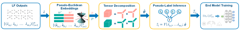
3.1 Pseudo-Euclidean Embeddings

Our first task is to embed the metric space into a continuous space—enabling easier computation and potential dimensionality reduction. A standard approach is multi-dimensional scaling (MDS) [15], which embeds 𝒴\mathcal{Y} into d\mathbb{R}^{d}. A downside of MDS is that not all metric spaces embed (isometrically) into Euclidean space, as the square distance matrix 𝐃{\bf D} must be positive semi-definite.

A simple and elegant way to overcome this difficulty is to instead use pseudo-Euclidean spaces for embeddings. These pseudo-spaces do not require a p.s.d. inner product. As an outcome, any finite metric space can be embedded into a pseudo-Euclidean space with no distortion [11]—so that distances are exactly preserved. Such spaces have been applied to similarity-based learning methods [21, 17, 19]. A vector 𝐮{\bf u} in a pseudo-Euclidean space d+,d\mathbb{R}^{d^{+},d^{-}} has two parts: 𝐮+d+{\bf u}^{+}\in\mathbb{R}^{d^{+}} and 𝐮d{\bf u}^{-}\in\mathbb{R}^{d^{-}}. The dot product and the squared distance between any two vectors 𝐮,𝐯{\bf u},{\bf v} are 𝐮,𝐯ϕ=𝐮+,𝐯+𝐮,𝐯\langle{\bf u},{\bf v}\rangle_{\phi}=\langle{\bf u}^{+},{\bf v}^{+}\rangle-\langle{\bf u}^{-},{\bf v}^{-}\rangle and dϕ2(𝐮,𝐯)=𝐮+𝐯+22𝐮𝐯22d^{2}_{\phi}({\bf u},{\bf v})=||{\bf u}^{+}-{\bf v}^{+}||_{2}^{2}-||{\bf u}^{-}-{\bf v}^{-}||_{2}^{2}. These properties enable isometric embeddings: the distance can be decomposed into two components that are individually induced from p.s.d. inner products—and can thus be embedded via MDS. Indeed, pseudo-Euclidean embeddings effectively run MDS for each component (see Algorithm 1 steps 4-9). To recover the original distance, we obtain 𝐮+𝐯+22||{\bf u}^{+}-{\bf v}^{+}||_{2}^{2} and 𝐮𝐯22||{\bf u}^{-}-{\bf v}^{-}||_{2}^{2} and subtract.

Example: To see why such embeddings are advantageous, we compare with a one-hot vector representation (whose dimension is |𝒴||\mathcal{Y}|). Consider a tree with a root node and three branches, each of which is a path with tt nodes. Let 𝒴\mathcal{Y} be the nodes in the tree with the shortest-hops distance as the metric. The pseudo-Euclidean embedding dimension is just d=3d=3; see Appendix for more details. The one-hot embedding dimension is d=|𝒴|=3t+1d=|\mathcal{Y}|=3t+1—arbitrarily larger!

Now we are ready to apply these embeddings to our problem. Abusing notation, we write 𝝀a\bm{\lambda}_{a} and 𝐲{\bf y} for the pseudo-Euclidean embeddings of λa,y\lambda_{a},y, respectively. We have that d𝒴2(λa,y)=dϕ2(𝝀a,𝐲)d^{2}_{\mathcal{Y}}(\lambda_{a},y)=d^{2}_{\phi}(\bm{\lambda}_{a},{\bf y}), so that there is no loss of information from working with these spaces. In addition, we write the mean as 𝝁a,y=𝔼[𝝀a|𝐲]\bm{\mu}_{a,y}=\mathbb{E}[\bm{\lambda}_{a}|{\bf y}] and the covariance as 𝚺a,y\bm{\Sigma}_{a,y}. Our goal is to obtain an accurate estimate 𝝁^a,y=𝔼^[𝝀a|𝐲]\hat{\bm{\mu}}_{a,y}=\hat{\mathbb{E}}[\bm{\lambda}_{a}|{\bf y}], which we will use to estimate the mean parameters 𝔼[d𝒴2(λa,y)]\mathbb{E}[d^{2}_{\mathcal{Y}}(\lambda_{a},y)]. If we could observe yy, it would be easy to empirically estimate 𝝁a,y\bm{\mu}_{a,y}—but we do not have access to it. Our approach will be to apply tensor decomposition for multi-view mixtures [2].

3.2 Multi-View Mixtures and Tensor Decompositions

In a multi-view mixture model, multiple views {λa}a=1m\{\lambda_{a}\}_{a=1}^{m} of a latent variable YY are observed. These views are independent when conditioned on YY. We treat the positive and negative components 𝝀a+d+\bm{\lambda}_{a}^{+}\in\mathbb{R}^{d^{+}} and 𝝀ad\bm{\lambda}_{a}^{-}\in\mathbb{R}^{d^{-}} of our pseudo-Euclidean embedding as separate multi-view mixtures:

𝝀a+|𝐲𝝁a,y++σd+ϵa+ and 𝝀a|𝐲𝝁a,y+σdϵaa[m],\bm{\lambda}_{a}^{+}|{\bf y}\sim\bm{\mu}_{a,y}^{+}+\sigma\sqrt{d^{+}}\cdot\bm{\epsilon}_{a}^{+}\quad\text{ and }\quad\bm{\lambda}_{a}^{-}|{\bf y}\sim\bm{\mu}_{a,y}^{-}+\sigma\sqrt{d^{-}}\cdot\bm{\epsilon}_{a}^{-}\qquad\forall a\in[m], (4)

where 𝝁a,y+=𝔼[𝝀a+|𝐲]\bm{\mu}^{+}_{a,y}=\mathbb{E}[\bm{\lambda}_{a}^{+}|{\bf y}], 𝝁a,y=𝔼[𝝀a|𝐲]\bm{\mu}^{-}_{a,y}=\mathbb{E}[\bm{\lambda}_{a}^{-}|{\bf y}] and ϵa+,ϵa\bm{\epsilon}_{a}^{+},\bm{\epsilon}_{a}^{-} are mean zero random vectors with covariances 1d+𝐈d+,1d𝐈d\frac{1}{d^{+}}{\bf I}_{d^{+}},\frac{1}{d^{-}}{\bf I}_{d^{-}} respectively. Here σ2\sigma^{2} is a proxy variance whose use is described in Assumption 3.

1: Labeling function outputs 𝐋={(λ1,i,,λm,i)}i=1n{\bf L}=\{(\lambda_{1,i},\ldots,\lambda_{m,i})\}_{i=1}^{n}, Label Space 𝒴={y0,,yr1}\mathcal{Y}=\{y_{0},\ldots,y_{r-1}\}
2: Pseudolabels for each data point 𝐙={z~i}i=1n{\bf Z}=\{\tilde{z}_{i}\}_{i=1}^{n}
3:
4:\triangleright Step 1: Compute pseudo-Euclidean Embeddings
5:Construct matrices 𝐃r×r{\bf D}\in\mathbb{R}^{r\times r}, 𝐃ij=d𝒴2(yi,yj){\bf D}_{ij}=d^{2}_{\mathcal{Y}}(y_{i},y_{j}) and 𝐌r×r{\bf M}\in\mathbb{R}^{r\times r}, 𝐌ij=12(𝐃0i2+𝐃0j2𝐃ij2){\bf M}_{ij}=\frac{1}{2}({\bf D}_{0i}^{2}+{\bf D}_{0j}^{2}-{\bf D}_{ij}^{2})
6:Compute eigendecomposition of 𝐌{\bf M} and let 𝐌=𝐔𝐂𝐔T{\bf M}={\bf U}{\bf C}{\bf U}^{T}
7:Set l+,ll^{+},l^{-} be indices of positive and negative eigenvalues sorted by their magnitude
8:Let d+=|l+|,d=|l|d^{+}=|l^{+}|,\quad d^{-}=|l^{-}| i.e. the sizes of lists l+l^{+} and ll^{-} respectively.
9:Construct permutation matrix 𝐈permr×(d++d){\bf I}_{perm}\in\mathbb{R}^{r\times(d^{+}+d^{-})} by concatenating l+,ll^{+},l^{-} in order
10:𝐂¯=𝐂𝐈perm,𝐔¯=𝐔𝐈perm\bar{{\bf C}}={\bf C}{\bf I}_{perm},\bar{{\bf U}}={\bf U}{\bf I}_{perm}
11:𝕐=𝐔¯T𝐂¯12r×(d++d)\mathbb{Y}=\bar{{\bf U}}^{T}\bar{{\bf C}}^{\frac{1}{2}}\in\mathbb{R}^{r\times(d^{+}+d^{-})} and let this define the mapping g:𝒴𝕐g:\mathcal{Y}\mapsto\mathbb{Y}
12:
13:\triangleright Step 2: Parameter Estimation Using Tensor Decomposition
14:for a1a\leftarrow 1 to m3m-3 do
15:     Obtain embeddings 𝝀a,i=g(λa,i),𝝀b,i=g(λb,i),𝝀c,i=g(λc,i)i[n]\bm{\lambda}_{a,i}=g(\lambda_{a,i}),\bm{\lambda}_{b,i}=g(\lambda_{b,i}),\bm{\lambda}_{c,i}=g(\lambda_{c,i})\quad\forall i\in[n] where a,b,ca,b,c are uncorrelated
16:     Construct tensors 𝐓^+\hat{{\bf T}}^{+} and 𝐓^\hat{{\bf T}}^{-} as defined in (5) for triplet (a,b,c)(a,b,c)
17:     𝝁^a,y+,𝝁^b,y+,𝝁^c,y+\hat{\bm{\mu}}_{a,y}^{+},\hat{\bm{\mu}}_{b,y}^{+},\hat{\bm{\mu}}_{c,y}^{+} = TensorDecomposition(𝐓^+\hat{{\bf T}}^{+})
18:     𝝁^a,y,𝝁^b,y,𝝁^c,y\hat{\bm{\mu}}_{a,y}^{-},\hat{\bm{\mu}}_{b,y}^{-},\hat{\bm{\mu}}_{c,y}^{-} = TensorDecomposition(𝐓^\hat{{\bf T}}^{-})
19:     sa,y+=minz{1,+1}ϕ(z𝝁^a,y+,𝐲+)s^{+}_{a,y}=\min_{z\in\{-1,+1\}}\phi(z\cdot\hat{\bm{\mu}}^{+}_{a,y},{\bf y}^{+}) and similarly sb,y+,sc,y+,sa,y,sb,y,sc,ys^{+}_{b,y},s^{+}_{c,y},s^{-}_{a,y},s^{-}_{b,y},s^{-}_{c,y}
20:     𝝁^a,y+=sa,y+𝝁^a,y+\hat{\bm{\mu}}^{+}_{a,y}=s^{+}_{a,y}\cdot\hat{\bm{\mu}}^{+}_{a,y} and similarly correct signs of 𝝁^b,y+,𝝁^c,y+,𝝁^a,y,𝝁^b,y,𝝁^c,y\hat{\bm{\mu}}^{+}_{b,y},\hat{\bm{\mu}}^{+}_{c,y},\hat{\bm{\mu}}^{-}_{a,y},\hat{\bm{\mu}}^{-}_{b,y},\hat{\bm{\mu}}^{-}_{c,y}
21:
22:\triangleright Step 3: Infer Pseudo-Labels
23:Z~(i)=z~iY|λa=λa(i),λm=λm(i);𝜽^\tilde{Z}^{(i)}=\tilde{z}_{i}\sim Y|\lambda_{a}=\lambda_{a}^{(i)},\ldots\lambda_{m}=\lambda_{m}^{(i)};\hat{\bm{\theta}}
24:
25:return {z~i}i=1n\{\tilde{z}_{i}\}_{i=1}^{n}
Algorithm 1 Algorithm for Pseudolabel Construction

We cannot directly estimate these parameters from observations of 𝝀a\bm{\lambda}_{a}, due to the fact that 𝐲{\bf y} is not observed. However, we can observe various moments of the outputs of the LFs such as tensors of outer products of LF triplets. We require that for each aa such a triplet exists. Then,

𝐓+:=𝔼[𝝀a+𝝀b+𝝀c+]=y𝒴swy𝝁a,y+𝝁b,y+𝝁c,y+ and 𝐓^+:=1ni=1n𝝀a,i+𝝀b,i+𝝀c,i+.{\bf T}^{+}\vcentcolon=\mathbb{E}[\bm{\lambda}_{a}^{+}\otimes\bm{\lambda}_{b}^{+}\otimes\bm{\lambda}_{c}^{+}]=\sum_{y\in\mathcal{Y}_{s}}w_{y}\bm{\mu}_{a,y}^{+}\otimes\bm{\mu}_{b,y}^{+}\otimes\bm{\mu}_{c,y}^{+}\text{ and }\hat{{\bf T}}^{+}\vcentcolon=\frac{1}{n}\sum_{i=1}^{n}\bm{\lambda}_{a,i}^{+}\otimes\bm{\lambda}_{b,i}^{+}\otimes\bm{\lambda}_{c,i}^{+}. (5)

Here wyw_{y} are the mixture probabilities (prior probabilities of YY) and 𝒴s={y:wy>0}\mathcal{Y}_{s}=\{y:w_{y}>0\}. We similarly define 𝐓{\bf T}^{-} and 𝐓^\hat{{\bf T}}^{-}. We then obtain estimates 𝝁^a,y+,𝝁^a,y\hat{\bm{\mu}}_{a,y}^{+},\hat{\bm{\mu}}_{a,y}^{-} using an algorithm from [1] with minor modifications to handle pseudo-Euclidean rather than Euclidean space. The overall approach is shown in Algorithm 1. We have three key assumptions for our analysis,

Assumption 1.

The support of PYP_{Y}, i.e., k=|{y:wy>0}|k=|\{y:w_{y}>0\}| and the label space 𝒴\mathcal{Y} is such that min(d+,d)k\min(d^{+},d^{-})\geq k, 𝛍a,y+2=1,𝛍a,y2=1||\bm{\mu}^{+}_{a,y}||_{2}=1,||\bm{\mu}^{-}_{a,y}||_{2}=1 for a[m],y𝒴a\in[m],y\in\mathcal{Y}.

Assumption 2.

(Bounded angle between 𝛍\bm{\mu} and 𝐲{\bf y}) Let ω(𝐮,𝐯)\omega({\bf u},{\bf v}) denote the angle between any two vectors 𝐮,𝐯{\bf u},{\bf v} in a Euclidean space. We assume that ω(𝛍a,y+,𝐲+)[0,π/2c)\omega(\bm{\mu}^{+}_{a,y},{\bf y}^{+})\in[0,\pi/2-c), ω(𝛍a,y,𝐲)[0,π/2c)\omega(\bm{\mu}^{-}_{a,y},{\bf y}^{-})\in[0,\pi/2-c) a[m]\forall a\in[m], and y𝒴sy\in\mathcal{Y}_{s}, for some sufficiently small c(0,π/4]c\in(0,\pi/4] such that sin(c)max(ϵ0(d+),ϵ0(d))\sin(c)\geq\max(\epsilon_{0}(d^{+}),\epsilon_{0}(d^{-})), where ϵ0(d)\epsilon_{0}(d) is defined for some n>n0n>n_{0} samples in (6).

Assumption 3.

σ\sigma is such that the recovery error with model (4) is at least as large as with (3) .

These enable providing guarantees on recovering the mean vector magnitudes (1) and signs (2) and simplify the analysis (1), (3); all three can be relaxed at the expense of a more complex analysis.

Our first theoretical result shows that we have near-consistency in estimating the mean parameters in (3). We use standard notation 𝒪~\tilde{\mathcal{O}} ignoring logarithmic factors.

Theorem 1.

Let 𝛍^a,y+,𝛍^a,y\hat{\bm{\mu}}^{+}_{a,y},\hat{\bm{\mu}}^{-}_{a,y} be the estimates of 𝛍a,y+,𝛍a,y{\bm{\mu}}^{+}_{a,y},{\bm{\mu}}^{-}_{a,y} returned by Algorithm 1 with input 𝐓^+,𝐓^\hat{{\bf T}}^{+},\hat{{\bf T}}^{-} constructed using isometric pseudo-Euclidean embeddings (in d+,d\mathbb{R}^{d^{+},d^{-}}). Suppose Assumptions 1 and 2 are met, a sufficiently large number of samples nn are drawn from the model in  (3), and k=|𝒴s|k=|\mathcal{Y}_{s}|. Then there exists a constant C0>0C_{0}>0 such that with high probability a[m]\forall a\in[m] and y𝒴sy\in\mathcal{Y}_{s},

|θaθ^a|C0|𝔼[d𝒴2(λa,y)]𝔼^[d𝒴2(λa,y)]|ϵ(d+)+ϵ(d),\displaystyle|\theta_{a}-\hat{\theta}_{a}|\leq C_{0}\Big{|}\mathbb{E}[d^{2}_{\mathcal{Y}}(\lambda_{a},y)]-\hat{\mathbb{E}}[d^{2}_{\mathcal{Y}}(\lambda_{a},y)]\Big{|}\leq\epsilon(d^{+})+\epsilon(d^{-}),

where

ϵ(d):={𝒪~(kdn)+𝒪~(kd) if σ2=Θ(1),𝒪~(kn)+𝒪~(kd) if σ2=Θ(1d).\epsilon(d)\vcentcolon=\begin{cases}\tilde{\mathcal{O}}\Big{(}k\sqrt{\frac{d}{n}}\Big{)}+\tilde{\mathcal{O}}\Big{(}\frac{\sqrt{k}}{d}\Big{)}\quad&\text{ if }\,\sigma^{2}=\Theta(1),\\ \tilde{\mathcal{O}}\Big{(}\sqrt{\frac{k}{n}}\Big{)}+\tilde{\mathcal{O}}\Big{(}\frac{\sqrt{k}}{d}\Big{)}\quad&\text{ if }\,\sigma^{2}=\Theta(\frac{1}{d}).\end{cases} (6)

We interpret Theorem 6. It is a nearly direct application of [2]. There are two noise cases for σ\sigma. In the high-noise case, σ\sigma is independent of dimension dd (and thus |𝒴||\mathcal{Y}|). Intuitively, this means the average distance balls around each LF begin to overlap as the number of points grows—explaining the multiplicative kk term. If the noise scales down as we add more embedded points, this problem is removed, as in the low-noise case. In both cases, the second error term comes from using the algorithm of [1] and is independent of the sampling error. Since k=Θ(d)k=\Theta(d), this term goes down with dd. The first error term is due to sampling noise and goes to zero in the number of samples nn. Note the tradeoffs of using the embeddings. If we used one-hot encoding, d=|𝒴|d=|\mathcal{Y}|, and in the high-noise case, we would pay a very heavy cost for d/n\sqrt{d/n}. However, while sampling error is minimized when using a very small dd, we pay a cost in the second error term. This leads to a tradeoff in selecting the appropriate embedding dimension.

4 Generalization Error for Structured Prediction in Finite Metric Spaces

We have access to labeling function outputs λ1,i,,λm,i\lambda_{1,i},\ldots,\lambda_{m,i} for points xix_{i} and noise rate estimates θ^a,,θ^m\hat{\theta}_{a},\ldots,\hat{\theta}_{m}. How can we use these to infer unobserved labels yy in (2)? Our approach is based on [18, 31],where the underlying loss function is modified to deal with noise. Analogously, we modify (2) in such a way that the generalization guarantee is nearly preserved.

4.1 Prediction with Pseudolabels

First, we construct the posterior distribution P𝜽^(Y=y|λ)P_{\hat{\bm{\theta}}}(Y=y|\lambda). We use our estimated noise model P𝜽^(λ|Y)P_{\hat{\bm{\theta}}}(\lambda|Y) and the prior P(Y=y)P(Y=y). We create pseudo-labels for each data point by drawing a random sample from the posterior distribution conditioned on the output of labeling functions: Z~(i)=z~iY|λa=λa(i),,λm=λm(i);𝜽^.\tilde{Z}^{(i)}=\tilde{z}_{i}\sim Y|\lambda_{a}=\lambda_{a}^{(i)},\ldots,\lambda_{m}=\lambda_{m}^{(i)};\hat{\bm{\theta}}. We thus observe (x1,z~1),,(xn,z~n)(x_{1},\tilde{z}_{1}),\ldots,(x_{n},\tilde{z}_{n}) where z~i\tilde{z}_{i} is sampled as above. To overcome the effect of noise we create a perturbed version of the distance function using the noise rates, generalizing [18]. This requires us to characterize the noise distribution induced by our inference procedure. In particular we seek the probability that Z~=yj\tilde{Z}=y_{j} when the true label is yjy_{j}. This can be expressed as follows. Let 𝒴m\mathcal{Y}^{m} denote the mm-fold Cartesian product of 𝒴\mathcal{Y} and let Λu=(λ1(u),,λm(u))\Lambda_{u}=(\lambda_{1}^{(u)},\ldots,\lambda_{m}^{(u)}) denote its uthu^{th} entry. We write

𝐏ij=P𝜽(Z~=yj|Y=yi)=u=1|𝒴m|P𝜽(Z~=yj|Λ=Λ(u))P𝜽(Λ=Λ(u)|Y=yi).{\bf P}_{ij}=P_{\bm{\theta}}(\tilde{Z}=y_{j}|Y=y_{i})=\sum_{u=1}^{|\mathcal{Y}^{m}|}P_{\bm{\theta}}(\tilde{Z}=y_{j}|\Lambda=\Lambda^{(u)})\cdot P_{\bm{\theta}}(\Lambda=\Lambda^{(u)}|Y=y_{i}). (7)

We define 𝐐ij=P𝜽^(Z~=yj|Y=yi){\bf Q}_{ij}=P_{\hat{\bm{\theta}}}(\tilde{Z}=y_{j}|Y=y_{i}) using 𝜽^\hat{\bm{\theta}}. 𝐏{\bf P} is the noise distribution induced by the true parameters 𝜽\bm{\theta} and 𝐐{\bf Q} is an approximation obtained from inference with the estimated parameters 𝜽^\hat{\bm{\theta}}. With this terminology, we can define the perturbed version of the distance function and a corresponding replacement of (2):

d~q(T,Y~=yj):=i=1k(𝐐1)jid𝒴2(T,Y=yi)yj𝒴s,\tilde{d}_{q}(T,\tilde{Y}=y_{j})\vcentcolon=\sum_{i=1}^{k}({\bf Q}^{-1})_{ji}d^{2}_{\mathcal{Y}}(T,Y=y_{i})\quad\forall y_{j}\in\mathcal{Y}_{s}, (8)
F~q(x,y):=1ni=1nαi(x)d~q(y,z~i)f^q(x)=argminy𝒴F~q(x,y).\tilde{F}_{q}(x,y)\vcentcolon=\frac{1}{n}\sum_{i=1}^{n}\alpha_{i}(x)\tilde{d}_{q}(y,\tilde{z}_{i})\qquad\hat{f}_{q}(x)=\arg\min_{y\in\mathcal{Y}}\tilde{F}_{q}(x,y). (9)

We similarly define d~p,F~p,f^p\tilde{d}_{p},\tilde{F}_{p},\hat{f}_{p} using the true noise distribution 𝐏{\bf P}. The perturbed distance d~p\tilde{d}_{p} is an unbiased estimator of the true distance. However we do not know the true noise distribution 𝐏{\bf P} hence we cannot use it for prediction. Instead we use d~q\tilde{d}_{q}. Note that d~q\tilde{d}_{q} is no longer an unbiased estimator—its bias can be expressed as function of the parameter recovery error bound in Theorem 6.

4.2 Bounding the Generalization Error

What can we say about the excess risk R(f^q)R(f)R(\hat{f}_{q})-R(f^{*})? Note that compared to the prediction based on clean labels, there are two additional sources of error. One is the noise in the labels (i.e., even if we know the true 𝐏{\bf P}, the quality of the pseudolabels is imperfect). The other is our estimation procedure for the noise distribution. We must address both sources of error.

Our analysis uses the following assumptions on the minimum and maximum singular values σmin(𝐏)\sigma_{\min}({\bf P}) , σmax(𝐏)\sigma_{\max}({\bf P}) and the condition number κ(𝐏)\kappa({\bf P}) of true noise matrix 𝐏{\bf P} and the function FF. Additional detail is provided in the Appendix.

Assumption 4.

(Noise model is not arbitrary) The true parameters 𝛉\bm{\theta} are such that σmin(𝐏)>0\sigma_{\min}({\bf P})>0, and the condition number κ(𝐏)\kappa({\bf P}) is sufficiently small.

Assumption 5.

(Normalized features) |α(x)|1|\alpha(x)|\leq 1, for all x𝒳x\in\mathcal{X}.

Assumption 6.

(Proxy strong convexity) The function FF in (2) satisfies the following property with some β>0\beta>0. As we move away from the minimizer of FF, the function increases and the rate of increase is proportional to the distance between the points:

F(x,f(x))F(x,f^(x))+βd𝒴2(f(x),f^(x))x𝒳,f.F\big{(}x,f(x)\big{)}\geq F\big{(}x,\hat{f}(x)\big{)}+\beta\cdot d_{\mathcal{Y}}^{2}\big{(}f(x),\hat{f}(x)\big{)}\qquad\forall x\in\mathcal{X},\forall f\in\mathcal{F}. (10)

With these assumptions, we provide a generalization result for prediction with pseudolabels,

Theorem 2.

(Generalization Error ) Let f^\hat{f} be the minimizer as defined in (2) over the clean labels and let f^q\hat{f}_{q} (defined in (9)) be the minimizer over the noisy labels obtained from inference in Algorithm 1. Suppose Assumptions 4,5,10 hold. Then for ϵ2=k5/2𝒪~(ϵ(d+)+ϵ(d))(1+κ(𝐏)σmin(𝐏))\epsilon_{2}=k^{5/2}\cdot\tilde{\mathcal{O}}(\epsilon(d^{+})+\epsilon(d^{-}))\cdot\Big{(}1+\frac{\kappa({\bf P})}{\sigma_{\min}({\bf P})}\Big{)} and c1=1+kσmin(𝐏)c_{1}=1+\frac{\sqrt{k}}{\sigma_{\min}({\bf P})}, with high probability,

R(f^q)R(f)+𝒪(n14)+𝒪~(c1βn12)+𝒪~(3ϵ2βn12).R(\hat{f}_{q})\leq R(f^{*})+\mathcal{O}(n^{-\frac{1}{4}})+\tilde{\mathcal{O}}\Big{(}\frac{c_{1}}{\beta}n^{-\frac{1}{2}}\Big{)}+\tilde{\mathcal{O}}\Big{(}\frac{3\epsilon_{2}}{\beta}n^{-\frac{1}{2}}\Big{)}. (11)

Implications and Tradeoffs:

We interpret each term in the bound. The first term is present even with access to the clean labels and hence unavoidable. The second term is the additional error we incur if we learn with the knowledge of the true noise distribution. The third term is due to the use of the estimated noise model. It is dominated by the noise rate recovery result in Theorem 6. If the third term goes to 0 (perfect recovery) then we obtain the rate 𝒪(n1/4)\mathcal{O}(n^{-1/4}), the same as in the case of access to clean labels. The third term is introduced by our noise rate recovery algorithm and has two terms: one dominated by 𝒪~(n1/2)\tilde{\mathcal{O}}(n^{-1/2}) and the other on 𝒪~(k/d)\tilde{\mathcal{O}}(\sqrt{k}/d) (see discussion of Theorem 6). Thus we only pay an extra additive factor 𝒪(k/d)\mathcal{O}(\sqrt{k}/d) in the excess risk when using pseudolabels.

5 Manifold-Valued Label Spaces: Noise Recovery and Generalization

We introduce a simple recovery method for weak supervision in constant-curvature Riemannian manifolds. First we briefly introduce some background notation on these spaces, then provide our estimator and consistency result, then the downstream generalization result. Finally, we discuss extensions to symmetric Riemannian manifolds, an even more general class of spaces.

Background on Riemannian manifolds

The following is necessarily a very abridged background; more detail can be found in [16, 30]. A smooth manifold MM is a space where each point is located in a neighborhood diffeomorphic to d\mathbb{R}^{d}. Attached to each point pp\in\mathcal{M} is a tangent space TpMT_{p}M; each such tangent space is a dd-dimensional vector space enabling the use of calculus.

A Riemannian manifold equips a smooth manifold with a Riemannian metric: a smoothly-varying inner product ,p\langle\cdot,\cdot\rangle_{p} at each point pp. This tool allows us to compute angles, lengths, and ultimately, distances d(p,q)d_{\mathcal{M}}(p,q) between points on the manifold as shortest-path distances. These shortest paths are called geodesics and can be parameterized as curves γ(t)\gamma(t), where γ(0)=p\gamma(0)=p, or by tangent vectors vTpMv\in T_{p}M. The exponential map operation exp:Tp\exp:T_{p}\mathcal{M}\rightarrow\mathcal{M} takes tangent vectors to manifold points. It enables switching between these tangent vectors: expp(v)=q\exp_{p}(v)=q implies that d(p,q)=vd_{\mathcal{M}}(p,q)=\|v\|.

Invariant

Our first contribution is a simple invariant that enables us to recover the error parameters. Note that we cannot rely on the finite metric-space technique, since the manifolds we consider have an infinite number of points. Nor do we need an embedding—we have a continuous representation as-is. Instead, we propose a simple idea based on the law of cosines. Essentially, on average, the geodesic triangle formed by the latent variable yy\in\mathcal{M} and two observed LFs λa,λb\lambda_{a},\lambda_{b}, is a right triangle. This means it can be characterized by the (Riemannian) version of the Pythagorean theorem:

Lemma 1.

For 𝒴=\mathcal{Y}=\mathcal{M}, a hyperbolic manifold, yPy\sim P for some distribution PP on \mathcal{M} and labeling functions λa,λb\lambda_{a},\lambda_{b} drawn from (3), 𝔼coshd𝒴(λa,λb)=𝔼coshd𝒴(λb,y)𝔼coshd𝒴(λb,y)\mathbb{E}\cosh d_{\mathcal{Y}}(\lambda_{a},\lambda_{b})=\mathbb{E}\cosh d_{\mathcal{Y}}(\lambda_{b},y)\mathbb{E}\cosh d_{\mathcal{Y}}(\lambda_{b},y), while for 𝒴=\mathcal{Y}=\mathcal{M} a spherical manifold, 𝔼cosd𝒴(λa,λb)=𝔼cosd𝒴(λb,y)𝔼cosd𝒴(λb,y).\mathbb{E}\cos d_{\mathcal{Y}}(\lambda_{a},\lambda_{b})=\mathbb{E}\cos d_{\mathcal{Y}}(\lambda_{b},y)\mathbb{E}\cos d_{\mathcal{Y}}(\lambda_{b},y).

These invariants enable us to easily learn by forming a triplet system. Suppose we construct the equation in Lemma 1 for three pairs of labeling functions. The resulting system can be solved to express 𝔼[cosh(d𝒴(λa,y))]\mathbb{E}[\cosh(d_{\mathcal{Y}}(\lambda_{a},y))] in terms of 𝔼cosh(d𝒴(λa,λb)),𝔼cosh(d𝒴(λa,λc)),𝔼cosh(d𝒴(λb,λc))\mathbb{E}\cosh(d_{\mathcal{Y}}(\lambda_{a},\lambda_{b})),\mathbb{E}\cosh(d_{\mathcal{Y}}(\lambda_{a},\lambda_{c})),\mathbb{E}\cosh(d_{\mathcal{Y}}(\lambda_{b},\lambda_{c})). Specifically,

𝔼cosh(d𝒴(λa,y))=𝔼coshd𝒴(λa,λb)𝔼coshd𝒴(λa,λc)(𝔼cosh(d𝒴(λb,λc))2.{\mathbb{E}}\cosh(d_{\mathcal{Y}}(\lambda_{a},y))=\sqrt{\frac{{\mathbb{E}}\cosh d_{\mathcal{Y}}(\lambda_{a},\lambda_{b}){\mathbb{E}}\cosh d_{\mathcal{Y}}(\lambda_{a},\lambda_{c})}{({\mathbb{E}}\cosh(d_{\mathcal{Y}}(\lambda_{b},\lambda_{c}))^{2}}}.

Note that we can estimate 𝔼^\hat{\mathbb{E}} via the empirical versions of terms on the right , as these are based on observable quantities. This is a generalization of the binary case in [10] and the Gaussian (Euclidean) case in [28] to hyperbolic manifolds. A similar estimator can be obtained for spherical manifolds by replacing cosh\cosh with cos\cos.

Using this tool, we can obtain a consistent estimator for θa\theta_{a} for each of a=1,,ma=1,\ldots,m. Let C0C_{0} satisfy the following inequality 𝔼|𝔼^cosh(d𝒴(λa,λb))𝔼cosh(d𝒴(λa,λb))|C0𝔼|𝔼^d𝒴2(λa,λb))𝔼d𝒴2(λa,λb)|\mathbb{E}|\hat{\mathbb{E}}\cosh(d_{\mathcal{Y}}(\lambda_{a},\lambda_{b}))-\mathbb{E}\cosh(d_{\mathcal{Y}}(\lambda_{a},\lambda_{b}))|\geq C_{0}\mathbb{E}|\hat{\mathbb{E}}d_{\mathcal{Y}}^{2}(\lambda_{a},\lambda_{b}))-\mathbb{E}d_{\mathcal{Y}}^{2}(\lambda_{a},\lambda_{b})|; that is, C0C_{0} reflects the preservation of concentration when moving from distribution cosh(d)\cosh(d) to d2d^{2}. Then,

Theorem 3.

Let \mathcal{M} be a hyperbolic manifold. Fix 0<δ<10<\delta<1 and let Δ(δ)=minρPr(i,d𝒴(λa,i,λb,i))ρ)1δ\Delta(\delta)=\min_{\rho}\text{Pr}\Big{(}\forall i,d_{\mathcal{Y}}(\lambda_{a,i},\lambda_{b,i)})\leq\rho\Big{)}\geq 1-\delta. Then, there exists a constant C1C_{1} so that with probability at least 1δ1-\delta, 𝔼|𝔼^d𝒴2(λa,y))𝔼d𝒴2(λa,y)|C1cosh(Δ(δ))3/2/C02n.\mathbb{E}|\hat{\mathbb{E}}d_{\mathcal{Y}}^{2}(\lambda_{a},y))-\mathbb{E}d_{\mathcal{Y}}^{2}(\lambda_{a},y)|\leq{C_{1}\cosh(\Delta(\delta))^{3/2}}/{C_{0}\sqrt{2n}}.

As we hoped, our estimator is consistent. Note that we pay a price for a tighter bound: Δ(δ)\Delta(\delta) is large for smaller probability δ\delta. It is possible to estimate the size of Δ(δ)\Delta(\delta) (more generally, it is a function of the curvature). We provide more details in the Appendix.

Next, we adapt the downstream model predictor (2) in the following way. Let μ^a2=𝔼^[d𝒴2(λa,y)]\hat{\mu}_{a}^{2}=\hat{\mathbb{E}}[d_{\mathcal{Y}}^{2}(\lambda_{a},y)]. Let β=[β1,,βm]T\beta=[\beta_{1},\ldots,\beta_{m}]^{T} be such that aβa=1\sum_{a}\beta_{a}=1 and β\beta minimizes aβa2μ^a2\sum_{a}\beta_{a}^{2}\hat{\mu}_{a}^{2}. Then, we set

f~(x)=argminy𝒴1ni=1nαi(x)a=1mβa2d𝒴2(y,λa,i).\displaystyle\tilde{f}(x)=\operatorname*{arg\,min}_{y\in\mathcal{Y}}\frac{1}{n}\sum_{i=1}^{n}\alpha_{i}(x)\sum_{a=1}^{m}\beta_{a}^{2}d_{\mathcal{Y}}^{2}(y,\lambda_{a,i}).

We simply replace each of the true labels with a combination of the labeling functions. With this, we can state our final result. First, we introduce our assumptions.

Let q=argminz𝒴𝔼[α(x)(y)d𝒴2(z,y)]q=\operatorname*{arg\,min}_{z\in\mathcal{Y}}\mathbb{E}[\alpha(x)(y)d_{\mathcal{Y}}^{2}(z,y)], where the expectation is taken over the population level distribution and α(x)(y)\alpha(x)(y) denotes the kernel at yy.

Assumption 7.

(Bounded Hugging Function c.f. [29]) Let qq be defined as above. For all a,ba,b\in\mathcal{M}, the hugging function at qq is given by kqb(a)=1(logq(a)logq(b)2d𝒴2(a,b))/d𝒴2(q,b)k_{q}^{b}(a)=1-(\|\log_{q}(a)-\log_{q}(b)\|^{2}-d_{\mathcal{Y}}^{2}(a,b))/d_{\mathcal{Y}}^{2}(q,b). We assume that kqb(a)k_{q}^{b}(a) is lower bounded by kmink_{\min}.

Assumption 8.

(Kernel Symmetry) We assume that for all xx and all vTqv\in T_{q}\mathcal{M}, α(x)(expq(v))=α(x)(expq(v))\alpha(x)(\exp_{q}(v))=\alpha(x)(\exp_{q}(-v)).

The first condition provides control on how geodesic triangles behave; it relates to the curvature. We provide more details on this in the Appendix. The second assumption restricts us to kernels symmetric about the minimizers of the objective FF. Finally, suppose we draw (x,y)(x,y) and (x,y)(x^{\prime},y^{\prime}) independently from PXYP_{XY}. Set σo2=α(x)(y)𝔼d𝒴2(y,y)\sigma^{2}_{o}=\alpha(x)(y)\mathbb{E}d_{\mathcal{Y}}^{2}(y,y^{\prime}).

Theorem 4.

Let \mathcal{M} be a complete manifold and suppose the assumptions above hold. Then, there exist constants C3C_{3}, C4C_{4}

𝔼[d𝒴2(f^(x),f~(x))]C3σo2nkmin+C4a=1mβa2μ^a2mnkmin.\mathbb{E}[d_{\mathcal{Y}}^{2}(\hat{f}(x),\tilde{f}(x))]\leq\frac{C_{3}\sigma_{o}^{2}}{nk_{\min}}+\frac{C_{4}\sum_{a=1}^{m}\beta^{2}_{a}\hat{\mu}_{a}^{2}}{mnk_{\min}}.
Refer to caption
Refer to caption
Refer to caption
Figure 2: Finite metric space case. Parameter estimation improves with samples nn in learning to rank—showing nearly-consistent behavior. Our tensor decomposition estimator outperforms [28]. In particular, (top left) as the number of samples increases, our estimates of the positive and negative components of 𝐓\mathbf{T} improve. (Top right) the improvements in 𝐓\mathbf{T} recovery with more samples translates to significantly improved performance over [28], which is close to constant across nn. (Bottom) this improved parameter estimation further translates to improvements in label model accuracy (using only the noisy estimates for prediction, without training an end model) and end model generalization. For the top two plots, we use 𝜽=[6,3,8]\bm{\theta}=[6,3,8], and in the bottom plot, we use 𝜽=[0,0,1]\bm{\theta}=[0,0,1]. In all plots, we report medians along with upper and lower quartiles across 10 trials.

Note that as both mm and nn grow, as long as our worst-quality LF has bounded variance, our estimator of the true predictor is consistent. Moreover, we also have favorable dependence on the noise rate. This is because the only error we incur is in computing sub-optimal β\beta coefficients. We comment on this suboptimality in the Appendix.

A simple corollary of Theorem 4 provides the generalization guarantees we sought,

Corollary 1.

Let \mathcal{M} be a complete manifold and suppose the assumptions above hold. Then, with high probability, R(f~)R(f)+𝒪(n14).R(\tilde{f})\leq R(f^{*})+\mathcal{O}(n^{-\frac{1}{4}}).

Extensions to Other Manifolds

First, we note that all of our approaches almost immediately lift to products of constant-curvature spaces. For example, we have that 1×2\mathcal{M}_{1}\times\mathcal{M}_{2} has metric d𝒴2(p,q)=d12(p1,q1)+d22(p2,q2)d_{\mathcal{Y}}^{2}(p,q)=d^{2}_{\mathcal{M}_{1}}(p_{1},q_{1})+d^{2}_{\mathcal{M}_{2}}(p_{2},q_{2}), where pi,qip_{i},q_{i} are the projections of p,qp,q onto the iith component.

We can go beyond products of constant-curvature spaces as well. To do so, we can build generalizations of the law of cosines (as needed for the invariance in Lemma 1). For example, it is possible to do so for symmetric Riemannian manifolds using the tools in [3].

6 Experiments

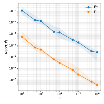
Finally, we validate our theoretical claims with experimental results demonstrating improved parameter recovery and end model generalization using our techniques over that of prior work [28]. We illustrate both the finite metric space and continuous space cases by targeting rankings (i.e., permutations) and hyperbolic spaces. In the case of rankings we show that our pseudo-Euclidean embeddings with tensor decomposition estimator yields stronger parameter recovery and downstream generalization than [28]. In the case of hyperbolic regression (an example of a Riemannian manifold), we show that our estimator yields improved parameter recovery over [28].

Finite metric spaces: Learning to rank

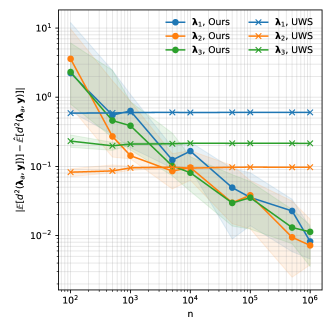
To experimentally evaluate our tensor decomposition estimator for finite metric spaces, we consider the problem of learning to rank. We construct a synthetic dataset whose ground truth comprises nn samples of two distinct rankings among the finite metric space of all length-four permutations. We construct three labeling functions by sampling rankings according to a Mallows model, for which we obtain pseudo-Euclidean embeddings to use with our tensor decomposition estimator.

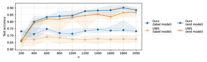
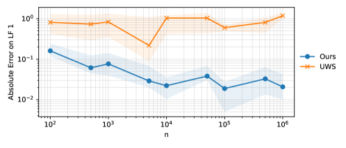
In Figure 2 (top left), we show that as we increase the number of samples, we can obtain an increasingly accurate estimate of 𝐓\mathbf{T}—exhibiting the nearly-consistent behavior predicted by our theoretical claims. This leads to downstream improvements in parameter estimates, which also become more accurate as nn increases. In contrast, we find that the estimates of the same parameters given by [28] do not improve substantially as nn increases, and are ultimately worse (see Figure 2, top right). Finally, this leads to improvements in the label model accuracy as compared to that of [28], and translates to improved accuracy of an end model trained using synthetic samples (see Figure 2, bottom).

Riemannian manifolds: Hyperbolic regression

We similarly evaluate our estimator using synthetic labels from a hyperbolic manifold, matching the setting of Section 5. As shown in Figure 3, we find that our estimator consistently outperforms that of [28], often by an order of magnitude.

Refer to caption
Figure 3: Continuous case. Parameter estimation improves with more samples in the hyperbolic regression problem. Our estimator outperforms [28]. Here, we use different randomly sampled values of 𝜽\bm{\theta} for each run. We report medians along with upper and lower quartiles across 10 trials.

7 Conclusion

We studied the theoretical properties of weak supervision applied to structured prediction in two general scenarios: label spaces that are finite metric spaces or constant-curvature manifolds. We introduced ways to estimate the noise rates of labeling functions, achieving consistency or near-consistency. Using these tools, we established that with suitable modifications downstream structured prediction models maintain generalization guarantees. Future directions include extending these results to even more general manifolds and removing some of the assumptions needed in our analysis.

Acknowledgments

We are grateful for the support of the NSF (CCF2106707), the American Family Funding Initiative and the Wisconsin Alumni Research Foundation (WARF).

References

  • AGH+ [14] Animashree Anandkumar, Rong Ge, Daniel Hsu, Sham M Kakade, and Matus Telgarsky. Tensor decompositions for learning latent variable models. Journal of Machine Learning Research, 15:2773–2832, 2014.
  • AGJ [14] Animashree Anandkumar, Rong Ge, and Majid Janzamin. Sample complexity analysis for learning overcomplete latent variable models through tensor methods. arXiv preprint arXiv:1408.0553, 2014.
  • AH [91] Helmer Aslaksen and Hsueh-Ling Huynh. Laws of trigonometry in symmetric spaces. Geometry from the Pacific Rim, 1991.
  • BDDH [14] Richard Baraniuk, Mark A Davenport, Marco F Duarte, and Chinmay Hegde. An introduction to compressive sensing. 2014.
  • BHS+ [07] Gükhan H. Bakir, Thomas Hofmann, Bernhard Schölkopf, Alexander J. Smola, Ben Taskar, and S. V. N. Vishwanathan. Predicting Structured Data (Neural Information Processing). The MIT Press, 2007.
  • BS [16] R.B. Bapat and Sivaramakrishnan Sivasubramanian. Squared distance matrix of a tree: Inverse and inertia. Linear Algebra and its Applications, 491:328–342, 2016.
  • CRR [16] Carlo Ciliberto, Lorenzo Rosasco, and Alessandro Rudi. A consistent regularization approach for structured prediction. In Advances in Neural Information Processing Systems 30 (NIPS 2016), volume 30, 2016.
  • Dem [92] James Demmel. The component-wise distance to the nearest singular matrix. SIAM Journal on Matrix Analysis and Applications, 13(1):10–19, 1992.
  • DRS+ [20] Jared A. Dunnmon, Alexander J. Ratner, Khaled Saab, Nishith Khandwala, Matthew Markert, Hersh Sagreiya, Roger Goldman, Christopher Lee-Messer, Matthew P. Lungren, Daniel L. Rubin, and Christopher Ré. Cross-modal data programming enables rapid medical machine learning. Patterns, 1(2), 2020.
  • FCS+ [20] Daniel Y. Fu, Mayee F. Chen, Frederic Sala, Sarah M. Hooper, Kayvon Fatahalian, and Christopher Ré. Fast and three-rious: Speeding up weak supervision with triplet methods. In Proceedings of the 37th International Conference on Machine Learning (ICML 2020), 2020.
  • Gol [85] Lev Goldfarb. A new approach to pattern recognition. Progress in Pattern Recognition 2, pages 241–402, 1985.
  • GS [19] Colin Graber and Alexander Schwing. Graph structured prediction energy networks. In Advances in Neural Information Processing Systems 33 (NeurIPS 2019), volume 33, 2019.
  • KAG [18] Anna Korba and Florence d’Alché-Buc Alexandre Garcia. A structured prediction approach for label ranking. In Advances in Neural Information Processing Systems 32 (NeurIPS 2018), volume 32, 2018.
  • KL [15] Volodymyr Kuleshov and Percy S Liang. Calibrated structured prediction. In Advances in Neural Information Processing Systems 28 (NIPS 2015), 2015.
  • KW [78] J.B. Kruskal and M. Wish. Multidimensional Scaling. Sage Publications, 1978.
  • Lee [00] John M. Lee. Introduction to Smooth Manifolds. Springer, 2000.
  • LRBM [06] Julian Laub, Volker Roth, Joachim M Buhmann, and Klaus-Robert Müller. On the information and representation of non-euclidean pairwise data. Pattern Recognition, 39(10):1815–1826, 2006.
  • NDRT [13] Nagarajan Natarajan, Inderjit S. Dhillon, Pradeep Ravikumar, and Ambuj Tewari. Learning with noisy labels. In Proceedings of the 26th International Conference on Neural Information Processing Systems - Volume 1, NIPS’13, page 1196–1204, 2013.
  • PHD+ [06] Elżbieta Pękalska, Artsiom Harol, Robert P. W. Duin, Barbara Spillmann, and Horst Bunke. Non-euclidean or non-metric measures can be informative. In Dit-Yan Yeung, James T. Kwok, Ana Fred, Fabio Roli, and Dick de Ridder, editors, Structural, Syntactic, and Statistical Pattern Recognition, pages 871–880, 2006.
  • PM [19] Alexander Petersen and Hans-Georg Müller. Fréchet regression for random objects with euclidean predictors. Annals of Statistics, 47(2):691–719, 2019.
  • PPD [01] Elżbieta Pękalska, Pavel Paclik, and Robert P.W. Duin. A generalized kernel approach to dissimilarity-based classification. Journal of Machine Learning Research, 2:175–211, 2001.
  • RBE+ [18] Alexander Ratner, Stephen H. Bach, Henry Ehrenberg, Jason Fries, Sen Wu, and Christopher Ré. Snorkel: Rapid training data creation with weak supervision. In Proceedings of the 44th International Conference on Very Large Data Bases (VLDB), Rio de Janeiro, Brazil, 2018.
  • RCMR [18] Alessandro Rudi, Carlo Ciliberto, GianMaria Marconi, and Lorenzo Rosasco. Manifold structured prediction. In Advances in Neural Information Processing Systems 32 (NeurIPS 2018), volume 32, 2018.
  • RHD+ [19] A. J. Ratner, B. Hancock, J. Dunnmon, F. Sala, S. Pandey, and C. Ré. Training complex models with multi-task weak supervision. In Proceedings of the AAAI Conference on Artificial Intelligence, Honolulu, Hawaii, 2019.
  • RNGS [20] Christopher Ré, Feng Niu, Pallavi Gudipati, and Charles Srisuwananukorn. Overton: A data system for monitoring and improving machine-learned products. In Proceedings of the 10th Annual Conference on Innovative Data Systems Research, 2020.
  • RSW+ [16] A. J. Ratner, Christopher M. De Sa, Sen Wu, Daniel Selsam, and C. Ré. Data programming: Creating large training sets, quickly. In Proceedings of the 29th Conference on Neural Information Processing Systems (NIPS 2016), Barcelona, Spain, 2016.
  • SLB [20] Esteban Safranchik, Shiying Luo, and Stephen Bach. Weakly supervised sequence tagging from noisy rules. In Proceedings of the AAAI Conference on Artificial Intelligence (AAAI), pages 5570–5578, Apr. 2020.
  • SLV+ [22] Changho Shin, Winfred Li, Harit Vishwakarma, Nicholas Carl Roberts, and Frederic Sala. Universalizing weak supervision. In International Conference on Learning Representations, 2022.
  • Str [20] Austin J. Stromme. Wasserstein Barycenters: Statistics and Optimization. MIT, 2020.
  • Tu [11] Loring W. Tu. An Introduction to Manifolds. Springer, 2011.
  • vRW [18] Brendan van Rooyen and Robert C. Williamson. A theory of learning with corrupted labels. Journal of Machine Learning Research, 18(228):1–50, 2018.
  • ZS [16] Hongyi Zhang and Suvrit Sra. First-order methods for geodesically convex optimization. In Conference on Learning Theory, COLT 2016, 2016.

Appendix

The Appendix is organized as follows. First, we provide a glossary that summarizes the notation we use throughout the paper. Afterwards, we provide the proofs for the finite-valued metric space cases. We continue with the proofs and additional discussion for the manifold-valued label spaces. Finally, we give some additional explanations for pseudo-Euclidean spaces.

Appendix A Glossary

The glossary is given in Table 1 below.

Symbol Definition
𝒳\mathcal{X} feature space
𝒴\mathcal{Y} label metric space
𝒴s\mathcal{Y}_{s} support of prior distribution on true labels
d𝒴d_{\mathcal{Y}} label metric (distance) function
x1,x2,,xnx_{1},x_{2},\ldots,x_{n} unlabeled datapoints from 𝒳\mathcal{X}
y1,y2,,yny_{1},y_{2},\ldots,y_{n} latent (unobserved) labels from 𝒴\mathcal{Y}
s1,s2,,sms_{1},s_{2},\ldots,s_{m} labeling functions / sources
λ1,λ2,,λm\lambda_{1},\lambda_{2},\ldots,\lambda_{m} output of labeling functions (LFs)
𝝀1,𝝀2,,𝝀m\bm{\lambda}_{1},\bm{\lambda}_{2},\ldots,\bm{\lambda}_{m} pseudo-Euclidean embeddings of LFs outputs
λa,i\lambda_{a,i} output of aath LF on iith data point xix_{i}
𝝀a,i\bm{\lambda}_{a,i} pseudo-Euclidean embedding of output of aath LF on iith data point xix_{i}
nn number of data points
mm number of LFs
kk size of the support of prior on 𝒴\mathcal{Y} i.e. k=|𝒴s|k=|\mathcal{Y}_{s}|
rr size of 𝒴\mathcal{Y} for the finite case
θa,θ^a\theta_{a},\hat{\theta}_{a} true and estimated canonical parameters of model in (3)
𝜽,𝜽^\bm{\theta},\hat{\bm{\theta}} true and estimated canonical parameters arranged as vectors
𝔼[d𝒴2(λa,y)]\mathbb{E}[d^{2}_{\mathcal{Y}}(\lambda_{a},y)] mean parameters in (3)
gg pseudo-Euclidean embedding mapping
𝐏{\bf P} true noise model Pij=P𝜽(Y~=yj|Y=yi)P_{ij}=P_{\bm{\theta}}(\tilde{Y}=y_{j}|Y=y_{i}) with true parameters 𝜽\bm{\theta}
𝐐{\bf Q} estimated noise model with parameters 𝜽^\hat{\bm{\theta}}, Qij=P𝜽^(Y~=yj|Y=yi)Q_{ij}=P_{\hat{\bm{\theta}}}(\tilde{Y}=y_{j}|Y=y_{i})
Λ\Lambda a random element in 𝒴m\mathcal{Y}^{m} the mm-fold Cartesian product of 𝒴\mathcal{Y}
Λ(u)\Lambda^{(u)} uuth element in 𝒴m\mathcal{Y}^{m}
𝝁a,y+,𝝁a,y\bm{\mu}_{a,y}^{+},\bm{\mu}_{a,y}^{-} means of distributions in (4) corresponding to d+,d\mathbb{R}^{d^{+}},\mathbb{R}^{d^{-}}
ϵ(d+),ϵ(d)\epsilon(d^{+}),\epsilon(d^{-}) error in recovering the mean parameters (6)
σ\sigma proxy noise variance in (4)
F(x,y)F(x,y) the score function in (2) with true labels
F~p(x,y),F~q(x,y)\tilde{F}_{p}(x,y),\tilde{F}_{q}(x,y) the score function in (9) with noisy labels from distributions 𝐏{\bf P} and 𝐐{\bf Q}
f^\hat{f} minimizer of FF defined in (2)
f^p,f^q\hat{f}_{p},\hat{f}_{q} minimizers of F~p,F~q\tilde{F}_{p},\tilde{F}_{q} as defined in (2)
σmax(𝐏)\sigma_{\max}({\bf P}) maximum singular value of 𝐏{\bf P}
σmin(𝐏)\sigma_{\min}({\bf P}) minimum singular value of 𝐏{\bf P}
κ(𝐏)\kappa({\bf P}) the condition number of matrix 𝐏{\bf P}
ω(𝐮,𝐯)\omega({\bf u},{\bf v}) angle between vectors 𝐮,𝐯d{\bf u},{\bf v}\in\mathbb{R}^{d}
Table 1: Glossary of variables and symbols used in this paper.

Appendix B Proofs for Parameter Estimation Error in Discrete Spaces

We introduce results leading to the proofs of the theorems for the finite-valued metric space case.

Lemma 2.

([2]) Let 𝐓^+,𝐓^\hat{{\bf T}}^{+},\hat{{\bf T}}^{-} be the third order observed moments for mutually independent labeling functions triplet, as defined in (5) using a sufficiently large number nn of i.i.d observations drawn from models in equation (4). Suppose there are sufficiently many such triplets to cover all labeling functions. Let 𝛍^a,y+,𝛍^a,y\hat{\bm{\mu}}_{a,y}^{+},\hat{\bm{\mu}}_{a,y}^{-} be the estimated parameters returned by the algorithm 1 for all a[m]a\in[m]. Let ϵ(d)\epsilon(d) be defined as above in equation (6), then the following holds with high probability for all labeling functions,

𝝁a,y+𝝁^a,y+2𝒪(ϵ(d+)) and 𝝁a,y𝝁^a,y2𝒪(ϵ(d))a[m]y𝒴s||\bm{\mu}_{a,y}^{+}-\hat{\bm{\mu}}_{a,y}^{+}||_{2}\leq\mathcal{O}(\epsilon(d^{+}))\quad\text{ and }\quad||\bm{\mu}_{a,y}^{-}-\hat{\bm{\mu}}_{a,y}^{-}||_{2}\leq\mathcal{O}(\epsilon(d^{-}))\quad\forall a\in[m]\,\,\forall y\in\mathcal{Y}_{s} (12)
Proof.

The result follows by first showing that our setting and assumptions imply that the conditions of Theorems 1 and 5 in [2] are satisfied, which allows us to adopt their results. We then translate the result in order to state it in terms of the 2\ell_{2} distance.

The tensor concentration result in Theorem 1 in [2] relies heavily on the noise matrices satisfying the Restricted Isometry Property (RIP) property. The authors make an explicit assumption that the noise model satisfies this condition. In our setting, we have a specific form of the noise model that allows us to show that this assumption is satisfied. The RIP condition is satisfied for sub-Gaussian noise matrices [4]. Our noise matrices are supported on a discrete space and have bounded entries, and so are sub-Gaussian.

The other required conditions on the norms of factor matrices and the number of latent factors are implied by Assumption 1. Thus, we can adopt the results on recovery of parameters 𝝁a,y\bm{\mu}_{a,y} and the prior weights wyw_{y} from [2]. The result gives us for all a[m],y𝒴sa\in[m],y\in\mathcal{Y}_{s},

dist(𝝁a,y+,𝝁^a,y+)𝒪(ϵ(d+)),dist(𝝁a,y,𝝁^a,y)𝒪(ϵ(d)),\text{dist}(\bm{\mu}_{a,y}^{+},\hat{\bm{\mu}}_{a,y}^{+})\leq\mathcal{O}\big{(}\epsilon(d^{+})\big{)},\quad\text{dist}(\bm{\mu}_{a,y}^{-},\hat{\bm{\mu}}_{a,y}^{-})\leq\mathcal{O}\big{(}\epsilon(d^{-})\big{)},

and

|wyw^y|𝒪(max(ϵ(d+),ϵ(d))/k),\quad|w_{y}-\hat{w}_{y}|\leq\mathcal{O}\Big{(}\max\big{(}\epsilon(d^{+}),\epsilon(d^{-})\big{)}/k\Big{)},

where dist(𝐮,𝐯)\text{dist}({\bf u},{\bf v}) is defined as follows. For any 𝐮,𝐯d{\bf u},{\bf v}\in\mathbb{R}^{d},

dist(𝐮,𝐯)=sup𝐳𝐮𝐳,𝐯𝐳2𝐯2=sup𝐳𝐯𝐳,𝐮𝐳2𝐮2.\text{dist}({\bf u},{\bf v})=\sup_{{\bf z}\perp{\bf u}}\frac{\langle{\bf z},{\bf v}\rangle}{||{\bf z}||_{2}||{\bf v}||_{2}}=\sup_{{\bf z}\perp{\bf v}}\frac{\langle{\bf z},{\bf u}\rangle}{||{\bf z}||_{2}||{\bf u}||_{2}}.

Next, we translate the result to the Euclidean distance. For 𝐮,𝐯d{\bf u},{\bf v}\in\mathbb{R}^{d} with 𝐮,𝐯=1||{\bf u}||,||{\bf v}||=1, it is easy to see that

minz{1,+1}z𝐮𝐯22dist(𝐮,𝐯).\min_{z\in\{-1,+1\}}||z{\bf u}-{\bf v}||_{2}\leq\sqrt{2}\,\text{dist}({\bf u},{\bf v}).

This notion of distance is oblivious to sign recovery. However, when sign recovery is possible then the Euclidean distance can be bounded as follows,

𝐮𝐯22dist(𝐮,𝐯).||{\bf u}-{\bf v}||_{2}\leq\sqrt{2}\,\text{dist}({\bf u},{\bf v}).

Next we make use of Assumption 2 to recover the signs of 𝝁+,𝝁\bm{\mu}^{+},\bm{\mu}^{-}. The assumption bounds the angle between true 𝝁a,y+\bm{\mu}_{a,y}^{+} and 𝐲+{\bf y}^{+} between [0,π/2c)[0,\pi/2-c) for some sufficiently small c(0,π/4]c\in(0,\pi/4] such that sin(c)>max(ϵ0(d+),ϵ0(d))\sin(c)>\max(\epsilon_{0}(d^{+}),\epsilon_{0}(d^{-})), where ϵ0(d)\epsilon_{0}(d) is defined for some n0<nn_{0}<n samples in equation (6). We measure ω(𝝁^a,y+,𝐲+)\omega(\hat{\bm{\mu}}_{a,y}^{+},{\bf y}^{+}) and ω(𝝁^a,y+,𝐲+)\omega(-\hat{\bm{\mu}}_{a,y}^{+},{\bf y}^{+}) and claim that whichever makes an acute angle with 𝐲+{\bf y}^{+} has the correct sign.

We have that ω(𝝁^a,y+,𝐲+)ω(𝝁^a,y+,𝝁a,y+)+ω(𝝁a,y+,𝐲+).\omega(\hat{\bm{\mu}}_{a,y}^{+},{\bf y}^{+})\leq\omega(\hat{\bm{\mu}}_{a,y}^{+},\bm{\mu}_{a,y}^{+})+\omega(\bm{\mu}_{a,y}^{+},{\bf y}^{+}). Let s{1,+1}s\in\{-1,+1\} be the correct sign, then,

ω(s𝝁^a,y+,𝐲+)\displaystyle\omega(s\hat{\bm{\mu}}_{a,y}^{+},{\bf y}^{+}) ω(s𝝁^a,y+,𝝁a,y+)+ω(s𝝁a,y+,𝐲+)\displaystyle\leq\omega(s\hat{\bm{\mu}}_{a,y}^{+},\bm{\mu}_{a,y}^{+})+\omega(s\bm{\mu}_{a,y}^{+},{\bf y}^{+})
sin1(ϵ(d+))+π/2c\displaystyle\leq\sin^{-1}(\epsilon(d^{+}))+\pi/2-c
<π/2(sin1(max(ϵ0(d+),ϵ0(d)))sin1(ϵ(d+)))\displaystyle<\pi/2-\Big{(}\sin^{-1}\big{(}\max(\epsilon_{0}(d^{+}),\epsilon_{0}(d^{-}))\big{)}-\sin^{-1}\big{(}\epsilon(d^{+})\big{)}\Big{)}
<π/2since sin1 is an increasing function in the domain under consideration.\displaystyle<\pi/2\quad\text{since }\sin^{-1}\text{ is an increasing function in the domain under consideration.}

With the correct sign sin1(ϵ(d+))<π/2\sin^{-1}(\epsilon(d^{+}))<\pi/2 and so is ω(s𝝁^a,y+,𝐲+)\omega(s\hat{\bm{\mu}}^{+}_{a,y},{\bf y}^{+}). Thus with incorrect sign ω(s𝝁^a,y+,𝐲+)>π/2\omega(-s\hat{\bm{\mu}}_{a,y}^{+},{\bf y}^{+})>\pi/2.

Hence, after disambiguating the signs we have,

𝝁a,y+𝝁^a,y+2𝒪(dist(𝝁a,y+,𝝁a,y))𝒪(ϵ(d+))||\bm{\mu}_{a,y}^{+}-\hat{\bm{\mu}}_{a,y}^{+}||_{2}\leq\mathcal{O}(\text{dist}(\bm{\mu}_{a,y}^{+},\bm{\mu}_{a,y}^{-}))\leq\mathcal{O}(\epsilon(d^{+}))

and similarly for 𝝁a,y\bm{\mu}^{-}_{a,y}. Next with n,dn,d sufficiently large such that ϵ(d+),ϵ(d)1\epsilon(d^{+}),\epsilon(d^{-})\leq 1, the result holds for squared distances. ∎

See 1

Proof.

We prove this by using the bounds on errors in the estimates of 𝝁a,y+\bm{\mu}^{+}_{a,y} and 𝝁a,y\bm{\mu}^{-}_{a,y} from Lemma 12. We proceed by bounding the errors in two parts for 𝔼[dϕ2(𝝀a+,𝐲+)]\mathbb{E}[d^{2}_{\phi}(\bm{\lambda}_{a}^{+},{\bf y}^{+})] and 𝔼[dϕ2(𝝀a,𝐲)]\mathbb{E}[d^{2}_{\phi}(\bm{\lambda}_{a}^{-},{\bf y}^{-})] separately and then combine them to get the bound on overall parameter estimation error.

We first bound the error for 𝔼[dϕ2(𝝀a+,𝐲+)]\mathbb{E}[d^{2}_{\phi}(\bm{\lambda}_{a}^{+},{\bf y}^{+})]. The true mean parameter (i.e., the true expected squared distance) can be expanded as follows:

𝔼[dϕ2(𝝀a+,𝐲+)]\displaystyle\mathbb{E}[d^{2}_{\phi}(\bm{\lambda}_{a}^{+},{\bf y}^{+})] =𝔼[𝝀a+22+𝐲+222𝝀a+,𝐲+],\displaystyle=\mathbb{E}\Big{[}||\bm{\lambda}_{a}^{+}||_{2}^{2}+||{\bf y}^{+}||_{2}^{2}-2\langle\bm{\lambda}_{a}^{+},{\bf y}^{+}\rangle\Big{]},
=𝔼𝝀[𝝀a+22]+𝔼𝐲[𝐲+22]2𝔼𝐲[𝝁a,y+,𝐲+].\displaystyle=\mathbb{E}_{\bm{\lambda}}[||\bm{\lambda}_{a}^{+}||_{2}^{2}]+\mathbb{E}_{{\bf y}}[||{\bf y}^{+}||_{2}^{2}]-2\mathbb{E}_{{\bf y}}[\langle\bm{\mu}_{a,y}^{+},{\bf y}^{+}\rangle].

The estimate 𝔼^𝝀[𝝀a+22]\hat{\mathbb{E}}_{\bm{\lambda}}[||\bm{\lambda}_{a}^{+}||_{2}^{2}] is computed empirically. The first term is estimated observed LF outputs, i.e. 𝔼^𝝀[𝝀a+22]=1ni=1n𝝀a(i),+22\hat{\mathbb{E}}_{\bm{\lambda}}[||\bm{\lambda}_{a}^{+}||_{2}^{2}]=\frac{1}{n}\sum_{i=1}^{n}||\bm{\lambda}_{a}^{(i),+}||_{2}^{2}. The second term is computed by using the estimated prior on the labels and for the last term we plug in the estimate of 𝝁a,y+\bm{\mu}_{a,y}^{+} computed using the tensor-decomposition algorithm. Putting them all together we have the following estimator:

𝔼^[dϕ2(𝝀a+,𝐲+)]\displaystyle\hat{\mathbb{E}}[d^{2}_{\phi}(\bm{\lambda}_{a}^{+},{\bf y}^{+})] =𝔼^𝝀[𝝀a+22]+𝔼^𝐲[𝐲+22]2𝔼^𝐲𝝁^a,y+,𝐲+.\displaystyle=\hat{\mathbb{E}}_{\bm{\lambda}}[||\bm{\lambda}_{a}^{+}||_{2}^{2}]+\hat{\mathbb{E}}_{{\bf y}}[||{\bf y}^{+}||_{2}^{2}]-2\hat{\mathbb{E}}_{{\bf y}}\langle\hat{\bm{\mu}}_{a,y}^{+},{\bf y}^{+}\rangle.

We want to bound the error of our estimator i.e. the difference |𝔼[dϕ2(𝝀a+,𝐲)]𝔼^[dϕ2(𝝀a+,𝐲)]||\mathbb{E}[d^{2}_{\phi}(\bm{\lambda}_{a}^{+},{\bf y})]-\hat{\mathbb{E}}[d^{2}_{\phi}(\bm{\lambda}_{a}^{+},{\bf y})]|. For this first consider the following,

|𝔼𝐲𝝁a,y+,𝐲+𝔼^𝐲𝝁^a,y+,𝐲+|\displaystyle|\mathbb{E}_{\bf y}\langle\bm{\mu}_{a,y}^{+},{\bf y}^{+}\rangle-\hat{\mathbb{E}}_{{\bf y}}\langle\hat{\bm{\mu}}_{a,y}^{+},{\bf y}^{+}\rangle| =y|(wy𝝁a,y+w^y𝝁^a,y+),𝐲+|\displaystyle=\sum_{y}\Big{|}\big{\langle}\big{(}w_{y}\bm{\mu}^{+}_{a,y}-\hat{w}_{y}\hat{\bm{\mu}}^{+}_{a,y}\big{)},{\bf y}^{+}\big{\rangle}\Big{|}
=y|(wy𝝁a,y+wy𝝁^a,y++wy𝝁^a,y+w^y𝝁^a,y+),𝐲+|\displaystyle=\sum_{y}\Big{|}\big{\langle}\big{(}w_{y}\bm{\mu}^{+}_{a,y}-w_{y}\hat{\bm{\mu}}^{+}_{a,y}+w_{y}\hat{\bm{\mu}}^{+}_{a,y}-\hat{w}_{y}\hat{\bm{\mu}}^{+}_{a,y}\big{)},{\bf y}^{+}\big{\rangle}\Big{|}
y|wy(𝝁a,y+𝝁^a,y+),𝐲+|+y𝒪(ϵ(d+)/k)|𝝁^a,y+,𝐲+|\displaystyle\leq\sum_{y}\big{|}w_{y}\big{\langle}\big{(}\bm{\mu}^{+}_{a,y}-\hat{\bm{\mu}}^{+}_{a,y}\big{)},{\bf y}^{+}\big{\rangle}\big{|}+\sum_{y}\mathcal{O}(\epsilon(d^{+})/k)\big{|}\langle\hat{\bm{\mu}}_{a,y}^{+},{\bf y}^{+}\rangle\big{|}
y|wy(𝝁a,y+𝝁^a,y+),𝐲+|+𝒪(ϵ(d+))\displaystyle\leq\sum_{y}\big{|}w_{y}\big{\langle}\big{(}\bm{\mu}^{+}_{a,y}-\hat{\bm{\mu}}^{+}_{a,y}\big{)},{\bf y}^{+}\big{\rangle}\big{|}+\mathcal{O}(\epsilon(d^{+}))
ywy𝝁a,y+𝝁^a,y+2𝐲+2+𝒪(ϵ(d+))\displaystyle\leq\sum_{y}w_{y}||\bm{\mu}^{+}_{a,y}-\hat{\bm{\mu}}^{+}_{a,y}||_{2}||{\bf y}^{+}||_{2}+\mathcal{O}(\epsilon(d^{+}))
𝒪(ϵ(d+)).\displaystyle\leq\mathcal{O}(\epsilon(d^{+})).

Here we used 𝝁a,y+𝝁^a,y+2𝒪(ϵ(d+))||\bm{\mu}_{a,y}^{+}-\hat{\bm{\mu}}_{a,y}^{+}||_{2}\leq\mathcal{O}(\epsilon(d^{+})) and 𝝁a,y+2,𝝁^a,y+2=1,𝐲+21,𝝀a+221||\bm{\mu}_{a,y}^{+}||_{2},||\hat{\bm{\mu}}_{a,y}^{+}||_{2}=1,||{\bf y}^{+}||_{2}\leq 1,||\bm{\lambda}_{a}^{+}||_{2}^{2}\leq 1 and |wyw^y|𝒪(ϵ(d+))/k|w_{y}-\hat{w}_{y}|\leq\mathcal{O}(\epsilon(d^{+}))/k. Similarly,

|𝔼^𝐲[𝐲+22]𝔼𝐲[𝐲+22]|=|ywy𝐲+22w^y𝐲+22|y|wyw^y|𝐲+22𝒪(ϵ(d+))\displaystyle\big{|}\hat{\mathbb{E}}_{{\bf y}}[||{\bf y}^{+}||_{2}^{2}]-\mathbb{E}_{{\bf y}}[||{\bf y}^{+}||_{2}^{2}]\big{|}=\big{|}\sum_{y}w_{y}||{\bf y}^{+}||_{2}^{2}-\hat{w}_{y}||{\bf y}^{+}||_{2}^{2}\big{|}\leq\sum_{y}|w_{y}-\hat{w}_{y}|\cdot||{\bf y}^{+}||_{2}^{2}\leq\mathcal{O}(\epsilon(d^{+})) (13)

Hence the parameter estimator error,

|𝔼[dϕ2(𝝀a+,𝐲)]𝔼^[dϕ2(𝝀a+,𝐲)]|\displaystyle\Big{|}\mathbb{E}[d^{2}_{\phi}(\bm{\lambda}_{a}^{+},{\bf y})]-\hat{\mathbb{E}}[d^{2}_{\phi}(\bm{\lambda}_{a}^{+},{\bf y})]\Big{|} |𝔼𝝀[||𝝀a+||22𝔼^𝝀[||𝝀a+||22]|+2|𝔼𝐲𝝁a,y+,𝐲+𝔼^𝐲𝝁^a,y+,𝐲+|\displaystyle\leq\Big{|}\mathbb{E}_{\bm{\lambda}}[||\bm{\lambda}_{a}^{+}||_{2}^{2}-\hat{\mathbb{E}}_{\bm{\lambda}}[||\bm{\lambda}_{a}^{+}||_{2}^{2}]\Big{|}+2|\mathbb{E}_{\bf y}\langle\bm{\mu}_{a,y}^{+},{\bf y}^{+}\rangle-\hat{\mathbb{E}}_{{\bf y}}\langle\hat{\bm{\mu}}_{a,y}^{+},{\bf y}^{+}\rangle|
+|𝔼^𝐲[𝐲+22]𝔼𝐲[𝐲+22]|\displaystyle\hskip 142.26378pt+\big{|}\hat{\mathbb{E}}_{{\bf y}}[||{\bf y}^{+}||_{2}^{2}]-\mathbb{E}_{{\bf y}}[||{\bf y}^{+}||_{2}^{2}]\big{|}
𝒪(1/n)+𝒪(ϵ(d+))+𝒪(ϵ(d+))\displaystyle\leq\mathcal{O}(1/\sqrt{n})+\mathcal{O}(\epsilon(d^{+}))+\mathcal{O}(\epsilon(d^{+}))
𝒪(ϵ(d+)).\displaystyle\leq\mathcal{O}(\epsilon(d^{+})).

In the second step, we bound the first term by 𝒪(1/n)\mathcal{O}(1/\sqrt{n}) via standard concentration inequalities.

Doing the same calculations for 𝝀a\bm{\lambda}_{a}^{-}, we obtain

|𝔼[dϕ2(𝝀a,𝐲)]𝔼^[dϕ2(𝝀a,𝐲)]|𝒪(ϵ(d)).\displaystyle\Big{|}\mathbb{E}[d^{2}_{\phi}(\bm{\lambda}_{a}^{-},{\bf y})]-\hat{\mathbb{E}}[d^{2}_{\phi}(\bm{\lambda}_{a}^{-},{\bf y})]\Big{|}\leq\mathcal{O}(\epsilon(d^{-})).

The overall error in mean parameters is then

|𝔼[dϕ2(𝝀a,𝐲)]𝔼^[dϕ2(𝝀a,𝐲)]|\displaystyle\Big{|}\mathbb{E}[d^{2}_{\phi}(\bm{\lambda}_{a},{\bf y})]-\hat{\mathbb{E}}[d^{2}_{\phi}(\bm{\lambda}_{a},{\bf y})]\Big{|} |𝔼[dϕ2(𝝀a+,𝐲)]𝔼^[dϕ2(𝝀a+,𝐲)]|+\displaystyle\leq\Big{|}\mathbb{E}[d^{2}_{\phi}(\bm{\lambda}_{a}^{+},{\bf y})]-\hat{\mathbb{E}}[d^{2}_{\phi}(\bm{\lambda}_{a}^{+},{\bf y})]\Big{|}+
|𝔼[dϕ2(𝝀a,𝐲)]𝔼^[dϕ2(𝝀a,𝐲)]|,\displaystyle\qquad\Big{|}\mathbb{E}[d^{2}_{\phi}(\bm{\lambda}_{a}^{-},{\bf y})]-\hat{\mathbb{E}}[d^{2}_{\phi}(\bm{\lambda}_{a}^{-},{\bf y})]\Big{|},
𝒪(ϵ(d+))+𝒪(ϵ(d)).\displaystyle\leq\mathcal{O}(\epsilon(d^{+}))+\mathcal{O}(\epsilon(d^{-})).

Next, we use a known relation between the mean and the canonical parameters of the exponential model to get the result in terms of the canonical parameters:

|θaθ^a|1emin(Aa(θ))|𝔼[d𝒴2(λa,y)𝔼^[d𝒴2(λa,y)]|.|\theta_{a}-\hat{\theta}_{a}|\leq\frac{1}{e_{\min}(A_{a}(\theta))}\big{|}\mathbb{E}[d^{2}_{\mathcal{Y}}(\lambda_{a},y)-\hat{\mathbb{E}}[d^{2}_{\mathcal{Y}}(\lambda_{a},y)]\big{|}.

where Aa(θ)A_{a}{(\theta)} is the log partition function of the label model in (3) and emin(Aa)=infθΘd2dθ2Aa(θ)e_{\min}(A_{a})=\inf_{\theta\in\Theta}\frac{d^{2}}{d\theta^{2}}A_{a}(\theta) over the parameter space Θ\Theta. For more details see Lemma 8 from [10] and Theorem 4.3 in [28]. Letting C0=maxa[m]emin(Aa)C_{0}=\max_{a\in[m]}e_{\min}(A_{a}) concludes the proof. ∎

Appendix C Proofs for Generalization Error in Discrete Space

In this section we give the proof for the generalization error bound in the discrete label spaces. We first show that the perturbed (noise-aware) distance function dp~\tilde{d_{p}} is an unbiased estimator of the true distance. Using this we show that the noise aware score function F~p\tilde{F}_{p} is a good uniform approximation of the score function FF. Then we show that the minimizer f^p\hat{f}_{p} of F~p\tilde{F}_{p} is close to the minimizer f^\hat{f} and that this closeness depends on how well F~p\tilde{F}_{p} approximates FF. Next, showing that F~q\tilde{F}_{q} is a good uniform approximation of F~p\tilde{F}_{p} using the results from previous section on parameter recovery leads to the result on generalization error of f^q\hat{f}_{q}.

Lemma 3.

Let the distribution Y~|Y\tilde{Y}|Y be given by 𝐏{\bf P} a k×kk\times k transition probability matrix with 𝐏ij=(Y~=yj|Y=yi){\bf P}_{ij}=\mathbb{P}(\tilde{Y}=y_{j}|Y=y_{i}) and suppose 𝐏{\bf P} is invertible. Let pseudo-distance d~p(T,Y~=yj):=i=1k(𝐏1)jid𝒴2(T,Y=yi)yj𝒴s,\tilde{d}_{p}(T,\tilde{Y}=y_{j})\vcentcolon=\sum_{i=1}^{k}({\bf P}^{-1})_{ji}d^{2}_{\mathcal{Y}}(T,Y=y_{i})\quad\forall y_{j}\in\mathcal{Y}_{s}, then,

𝔼Y~|Y=yi[d~p(T,Y~)]=d𝒴2(T,yi).\mathbb{E}_{\tilde{Y}|Y=y_{i}}\big{[}\tilde{d}_{p}(T,\tilde{Y})\big{]}=d_{\mathcal{Y}}^{2}(T,y_{i}). (14)
Proof.

Here we adopt the same ideas as in [18] to create the unbiased estimator d~p\tilde{d}_{p} as follows, First we write the equations for the expectations for each yiy_{i}. Which gives us a system of linear equations and solving them for d~p\tilde{d}_{p} gives us the expression for the unbiased estimator.

𝔼Y~|Y=yi[d~p(T,Y~)]=Pθ(Y~=y1|Y=yi)d~p(T,Y~=y1)++Pθ(Y~=yj|Y=yi)d~p(T,Y~=yj)+\displaystyle\mathbb{E}_{\tilde{Y}|Y=y_{i}}[\tilde{d}_{p}(T,\tilde{Y})]=P_{\theta}(\tilde{Y}=y_{1}|Y=y_{i})\tilde{d}_{p}(T,\tilde{Y}=y_{1})+\ldots+P_{\theta}(\tilde{Y}=y_{j}|Y=y_{i})\tilde{d}_{p}(T,\tilde{Y}=y_{j})+\ldots
+Pθ(Y~=yk|Y=yi)d~p(T,Y~=yk)=d𝒴2(T,yi)i[k]\displaystyle+P_{\theta}(\tilde{Y}=y_{k}|Y=y_{i})\tilde{d}_{p}(T,\tilde{Y}=y_{k})=d^{2}_{\mathcal{Y}}(T,y_{i})\quad\forall i\in[k]

Set 𝐝~pk\tilde{{\bf d}}_{p}\in\mathbb{R}^{k} with iith entry 𝐝~p[i]\tilde{{\bf d}}_{p}[i] given by d~p(T,Y~=yi)\tilde{d}_{p}(T,\tilde{Y}=y_{i}) and similarly define 𝐝{\bf d} with 𝐝[i]=d𝒴2(T,yi){\bf d}[i]=d^{2}_{\mathcal{Y}}(T,y_{i}). Then the above system of linear equations can be expressed as follows,

𝐏𝐝~p=𝐝𝐝~p=𝐏1𝐝d~p(T,Y~=yj)=i=1k(𝐏1)jid𝒴2(T,Y=yi)yj𝒴s{\bf P}\tilde{{\bf d}}_{p}={\bf d}\implies\tilde{{\bf d}}_{p}={\bf P}^{-1}{\bf d}\implies\tilde{d}_{p}(T,\tilde{Y}=y_{j})=\sum_{i=1}^{k}({\bf P}^{-1})_{ji}d^{2}_{\mathcal{Y}}(T,Y=y_{i})\forall y_{j}\in\mathcal{Y}_{s}

Next, we show that the noisy score function F~p\tilde{F}_{p} concentrates around the true score function FF for all xx and yy with high probability.

Lemma 4.

Let FF and F~p\tilde{F}_{p} be defined as in (9) and (2) over nn i.i.d. samples. Then the following holds for any x𝒳,y𝒴x\in\mathcal{X},y\in\mathcal{Y} with high probability,

|F(x,y)F~p(x,y)|𝒪~((1+kσmin(𝐏))1n)x𝒳,y𝒴s,|F(x,y)-\tilde{F}_{p}(x,y)|\leq\tilde{\mathcal{O}}\Big{(}\big{(}1+\frac{\sqrt{k}}{\sigma_{\min}({\bf P})}\big{)}\sqrt{\frac{1}{n}}\Big{)}\quad\forall x\in\mathcal{X},\forall y\in\mathcal{Y}_{s}, (15)

where σmin(𝐏)\sigma_{\min}({\bf P}) is the minimum singular value of 𝐏{\bf P}.

Proof.

Let {yi}i=1n\{y_{i}\}_{i=1}^{n} be the true labels of points {xi}i=1n\{x_{i}\}_{i=1}^{n} and let the pseudo-label for iith point drawn from the true noise model 𝐏{\bf P} be y~i\tilde{y}_{i}. Let 𝐝~pk\tilde{{\bf d}}_{p}\in\mathbb{R}^{k} be a vector such that its ithi^{th} entry is given as 𝐝~p[i]=d~p(T,Z~=yi)\tilde{{\bf d}}_{p}[i]=\tilde{d}_{p}(T,\tilde{Z}=y_{i}), and similarly and 𝐝k{\bf d}\in\mathbb{R}^{k} with 𝐝[i]=d𝒴2(T,Y=yi){\bf d}[i]=d^{2}_{\mathcal{Y}}(T,Y=y_{i}). Recall the definitions of the score functions FF and F~p\tilde{F}_{p} for any x𝒳x\in\mathcal{X} and yy in 𝒴\mathcal{Y},

F(x,y):=1ni=1nαi(x)d𝒴2(y,yi),F~p(x,y):=1ni=1nαi(x)d~p(y,y~i).\displaystyle F(x,y)\vcentcolon=\frac{1}{n}\sum_{i=1}^{n}\alpha_{i}(x)d^{2}_{\mathcal{Y}}(y,y_{i}),\qquad\tilde{F}_{p}(x,y)\vcentcolon=\frac{1}{n}\sum_{i=1}^{n}\alpha_{i}(x)\tilde{d}_{p}(y,\tilde{y}_{i}).

Taking their difference,

F~p(x,y)F(x,y)\displaystyle\tilde{F}_{p}(x,y)-F(x,y) =1ni=1nαi(x)(d~p(y,y~i)d𝒴2(y,yi)),\displaystyle=\frac{1}{n}\sum_{i=1}^{n}\alpha_{i}(x)\Big{(}\tilde{d}_{p}(y,\tilde{y}_{i})-d^{2}_{\mathcal{Y}}(y,y_{i})\Big{)},
=1ni=1nαi(x)ξ(y,yi,y~i).\displaystyle=\frac{1}{n}\sum_{i=1}^{n}\alpha_{i}(x)\xi(y,y_{i},\tilde{y}_{i}).

Here y,yiy,y_{i} are fixed and the randomness is over y~i\tilde{y}_{i}, thus we can think of y~i\tilde{y}_{i} as random variable Y~i\tilde{Y}_{i} and take the expectation of ξ\xi over the distribution 𝐏{\bf P}. From Lemma 14 we have 𝔼Y~|Y=yi[ξ(y,yi,Y~)]=0\mathbb{E}_{\tilde{Y}|Y=y_{i}}[\xi(y,y_{i},\tilde{Y})]=0 and this implies 𝔼[F~p(x,y)F(x,y)]=0\mathbb{E}[\tilde{F}_{p}(x,y)-F(x,y)]=0.

Moreover, αi(x)ξ(y,yi,Y~i)\alpha_{i}(x)\cdot\xi(y,y_{i},\tilde{Y}_{i}) are independent random variables and αi(x)1\alpha_{i}(x)\leq 1. The ξ\xi are bounded as follows as long as the spectral decomposition of 𝐏{\bf P} is not arbitrary,

maxz𝒴sd~p(y,z)=𝐝~p=𝐏1𝐝𝐏1𝐝.\max_{z\in\mathcal{Y}_{s}}\tilde{d}_{p}(y,z)=||\tilde{{\bf d}}_{p}||_{\infty}=||{\bf P}^{-1}{\bf d}||_{\infty}\leq||{\bf P}^{-1}||_{\infty}||{\bf d}||_{\infty}.

Now using the fact that 𝐝1||{\bf d}||_{\infty}\leq 1 and properties of matrix norms we get,

𝐏1𝐝𝐏1k𝐏12kσmin(𝐏).||{\bf P}^{-1}||_{\infty}||{\bf d}||_{\infty}\leq||{\bf P}^{-1}||_{\infty}\leq\sqrt{k}||{\bf P}^{-1}||_{2}\leq\frac{\sqrt{k}}{\sigma_{\min}({\bf P})}.

Moreover, y,z𝒴s,d𝒴2(y,z)1\forall y,z\in\mathcal{Y}_{s},d^{2}_{\mathcal{Y}}(y,z)\leq 1 which gives us the magnitude of random variables ξ(y,z,z~)\xi(y,z,\tilde{z}) is upper bounded by c1:=1+kσmin(𝐏)y,z,z~𝒴sc_{1}\vcentcolon=1+\frac{\sqrt{k}}{\sigma_{\min}({\bf P})}\,\forall y,z,\tilde{z}\in\mathcal{Y}_{s}. Thus using Hoeffding’s inequality and union bound over all y𝒴sy\in\mathcal{Y}_{s} we get,

|F~p(x,y)F(x,y)|𝒪~(c11n)y𝒴s,x𝒳.|\tilde{F}_{p}(x,y)-F(x,y)|\leq\tilde{\mathcal{O}}\Big{(}c_{1}\sqrt{\frac{1}{n}}\Big{)}\quad\forall y\in\mathcal{Y}_{s},x\in\mathcal{X}.

Note that, the statement holds for x𝒳x\in\mathcal{X} without requiring an explicit union bound over xx. It is because the above concentration depends only on the labels and the events that the above inequality does not hold for any distinct x1,x2𝒳x_{1},x_{2}\in\mathcal{X} are the same. ∎

Now, we show that the distance between minimizer of F~p\tilde{F}_{p} and FF is bounded.

Lemma 5.

Let f^\hat{f} be the minimizer as defined in (2) over the clean labels and let f^p\hat{f}_{p} (defined in eq. (9)) be the minimizer over the noisy labels obtained from conditional distribution Y~|Y\tilde{Y}|Y i.e. 𝐏{\bf P} such that lemma 14, 15 hold, and let the risk function be defined as in (1), then with high probability,

d𝒴2(f^p(x),f^(x))𝒪~(c1β1n)x𝒳.d^{2}_{\mathcal{Y}}\big{(}\hat{f}_{p}(x),\hat{f}(x)\big{)}\leq\tilde{\mathcal{O}}\Big{(}\frac{c_{1}}{\beta}\sqrt{\frac{1}{n}}\Big{)}\quad\forall x\in\mathcal{X}. (16)
Proof.

Recall the definitions,

f^(x)=argminy𝒴F(x,y)f^p(x)=argminy𝒴F~p(x,y)\displaystyle\hat{f}(x)=\operatorname*{arg\,min}_{y\in\mathcal{Y}}F(x,y)\qquad\hat{f}_{p}(x)=\operatorname*{arg\,min}_{y\in\mathcal{Y}}\tilde{F}_{p}(x,y)

Let d𝒴2(f1,f2)=supx𝒳d𝒴2(f1(x),f2(x))d^{2}_{\mathcal{Y}}(f_{1},f_{2})=\sup_{x\in\mathcal{X}}d^{2}_{\mathcal{Y}}\big{(}f_{1}(x),f_{2}(x)\big{)} and let (f^,r)={f:d𝒴2(f^,f)r}\mathcal{B}(\hat{f},r)=\{f:d^{2}_{\mathcal{Y}}(\hat{f},f)\leq r\} denote the ball of radius rr around f^\hat{f}.

From Lemma 15 we know for t=𝒪~(c11n),t=\tilde{\mathcal{O}}\Big{(}c_{1}\sqrt{\frac{1}{n}}\Big{)},

F(x,f(x))tF~p(x,f(x))F(x,f(x))+tf:𝒳𝒴s.\displaystyle F\big{(}x,f(x)\big{)}-t\leq\tilde{F}_{p}\big{(}x,f(x)\big{)}\leq F\big{(}x,f(x)\big{)}+t\quad\forall f:\mathcal{X}\mapsto\mathcal{Y}_{s}.

From Assumption 10 we have,

F(x,f(x))F(x,f^(x))+βd𝒴2(f(x),f^(x)).\displaystyle F\big{(}x,f(x)\big{)}\geq F\big{(}x,\hat{f}(x)\big{)}+\beta\cdot d_{\mathcal{Y}}^{2}(f(x),\hat{f}(x)).

Combining the two we get a lower bound on F~p\tilde{F}_{p},

F~p(x,f(x))F(x,f^(x))+βd𝒴2(f(x),f^(x))t.\displaystyle\tilde{F}_{p}(x,f(x))\geq F\big{(}x,\hat{f}(x)\big{)}+\beta\cdot d_{\mathcal{Y}}^{2}(f(x),\hat{f}(x))-t.

We want to find a sufficiently large ball around f^\hat{f} such that the minimizer of F~p\tilde{F}_{p} does not lie outside this ball. To see this let LBLB and UBUB denote the above mentioned lower and upper bounds on F~p\tilde{F}_{p},

LB(F~p,f,x)\displaystyle LB(\tilde{F}_{p},f,x) :=F(x,f^(x))+βd𝒴2(f(x),f^(x))t.\displaystyle\vcentcolon=F\big{(}x,\hat{f}(x)\big{)}+\beta\cdot d_{\mathcal{Y}}^{2}(f(x),\hat{f}(x))-t.
UB(F~p,f,x)\displaystyle UB(\tilde{F}_{p},f,x) :=F(x,f(x))+t.\displaystyle\vcentcolon=F\big{(}x,f(x)\big{)}+t.

For f(f^,2tβ)f\in\mathcal{B}(\hat{f},\frac{2t}{\beta}) and some ff^{\prime} such that

UB(F~p,f,x)\displaystyle UB(\tilde{F}_{p},f,x) LB(F~p,f,x)x,\displaystyle\leq LB(\tilde{F}_{p},f^{\prime},x)\quad\forall x,
F(x,f(x))+t\displaystyle F\big{(}x,f(x)\big{)}+t F(x,f^(x))+βd𝒴2(f(x),f^(x))t,\displaystyle\leq F\big{(}x,\hat{f}(x)\big{)}+\beta\cdot d_{\mathcal{Y}}^{2}(f^{\prime}(x),\hat{f}(x))-t,
F(x,f(x))F(x,f^(x))+t\displaystyle F\big{(}x,f(x)\big{)}-F\big{(}x,\hat{f}(x)\big{)}+t βd𝒴2(f(x),f^(x))t,\displaystyle\leq\beta\cdot d_{\mathcal{Y}}^{2}(f^{\prime}(x),\hat{f}(x))-t,
βd𝒴2(f(x),f^(x))+t\displaystyle\beta d^{2}_{\mathcal{Y}}(f(x),\hat{f}(x))+t βd𝒴2(f(x),f^(x))t,\displaystyle\leq\beta\cdot d_{\mathcal{Y}}^{2}(f^{\prime}(x),\hat{f}(x))-t,
d𝒴2(f(x),f^(x))\displaystyle d_{\mathcal{Y}}^{2}(f^{\prime}(x),\hat{f}(x)) 2t/β+d𝒴2(f(x),f^(x)).\displaystyle\geq 2t/\beta+d^{2}_{\mathcal{Y}}(f(x),\hat{f}(x)).

Thus considering the greatest lower bound, any ff^{\prime} with d𝒴2(f(x),f^(x))4tβd_{\mathcal{Y}}^{2}(f^{\prime}(x),\hat{f}(x))\geq\frac{4t}{\beta} cannot be the minimizer of F~p\tilde{F}_{p}, since there exists some other ff with smaller distance from f^\hat{f} that has smaller value compared to ff^{\prime}. ∎

Next we show that a good estimate of true noise matrix 𝐏{\bf P} by 𝐐{\bf Q} leads to F~q\tilde{F}_{q} being uniformly close to F~p\tilde{F}_{p}.

Lemma 6.

Let 𝐐{\bf Q}, 𝐏{\bf P} be the distributions defined in equation (7), and d~q(T,Y~)\tilde{d}_{q}(T,\tilde{Y}) be the distance function as in (8), if maxij|𝐏ij𝐐ij|=ϵ\max_{ij}|{\bf P}_{ij}-{\bf Q}_{ij}|=\epsilon,

|d~q(y,z~i)d~p(y,z~i)|𝒪(k2(σmax(𝐏)+κ(𝐏)σmin(𝐏))ϵ)y𝒴s.\big{|}\tilde{d}_{q}(y,\tilde{z}_{i})-\tilde{d}_{p}(y,\tilde{z}_{i})\big{|}\leq\mathcal{O}\Big{(}k^{2}\Big{(}\sigma_{\max}({\bf P})+\frac{\kappa({\bf P})}{\sigma_{\min}({\bf P})}\Big{)}\cdot\epsilon\Big{)}\qquad\forall y\in\mathcal{Y}_{s}. (17)
Proof.

Let 𝐝~qk\tilde{{\bf d}}_{q}\in\mathbb{R}^{k} be a vector such that its ithi^{th} entry is given as 𝐝~q[i]=d~q(T,Z~=yi)\tilde{{\bf d}}_{q}[i]=\tilde{d}_{q}(T,\tilde{Z}=y_{i}), and similarly, let 𝐝~pk\tilde{{\bf d}}_{p}\in\mathbb{R}^{k} with 𝐝~p[i]=d~p(T,Y~=yi),\tilde{{\bf d}}_{p}[i]=\tilde{d}_{p}(T,\tilde{Y}=y_{i}), and 𝐝k{\bf d}\in\mathbb{R}^{k} with 𝐝[i]=d𝒴2(T,Y=yi){\bf d}[i]=d^{2}_{\mathcal{Y}}(T,Y=y_{i}). It is easy to see that 𝐝~q=𝐐1𝐝\tilde{{\bf d}}_{q}={\bf Q}^{-1}{\bf d} and 𝐝~p=𝐏1𝐝\tilde{{\bf d}}_{p}={\bf P}^{-1}{\bf d}. Now consider the following expectation w.r.t 𝐏{\bf P},

𝐝~q𝐝~p=𝐐1𝐝𝐏1𝐝=(𝐐1𝐏1)𝐝.\displaystyle\tilde{{\bf d}}_{q}-\tilde{{\bf d}}_{p}={\bf Q}^{-1}{\bf d}-{\bf P}^{-1}{\bf d}=\big{(}{\bf Q}^{-1}-{\bf P}^{-1}\big{)}{\bf d}.

Let Δ𝐏=𝐏𝐐\Delta{\bf P}={\bf P}-{\bf Q}, and using standard matrix inversion results for small perturbations, [8], and 𝐝1||{\bf d}||_{\infty}\leq 1 we get the following. As maxij(Δ𝐏)ijϵ\max_{ij}(\Delta{\bf P})_{ij}\leq\epsilon, we have Δ𝐏2Δ𝐏Fϵk||\Delta{\bf P}||_{2}\leq||\Delta{\bf P}||_{F}\leq\epsilon k

𝐝~p𝐝~q\displaystyle||\tilde{{\bf d}}_{p}-\tilde{{\bf d}}_{q}||_{\infty} (𝐏+Δ𝐏)1𝐏1𝐝,\displaystyle\leq||({\bf P}+\Delta{\bf P})^{-1}-{\bf P}^{-1}||_{\infty}||{\bf d}||_{\infty},
k(𝐏+Δ𝐏)1𝐏12𝐝,\displaystyle\leq\sqrt{k}||({\bf P}+\Delta{\bf P})^{-1}-{\bf P}^{-1}||_{2}||{\bf d}||_{\infty},
=k(κ(𝐏)𝐏12Δ𝐏2)+k𝒪(Δ𝐏22),\displaystyle=\sqrt{k}\Big{(}\kappa({\bf P})||{\bf P}^{-1}||_{2}||\Delta{\bf P}||_{2}\Big{)}+\sqrt{k}\mathcal{O}(||\Delta{\bf P}||_{2}^{2}),
kκ(𝐏)𝐏12ϵk+𝒪(ϵ2k5/2),\displaystyle\leq\sqrt{k}\cdot\kappa({\bf P})||{\bf P}^{-1}||_{2}\cdot\epsilon k+\mathcal{O}(\epsilon^{2}k^{5/2}),
𝒪(k5/2(1+κ(𝐏)σmin(𝐏))ϵ)=:c2.\displaystyle\leq\mathcal{O}\Big{(}k^{5/2}\Big{(}1+\frac{\kappa({\bf P})}{\sigma_{\min}({\bf P})}\Big{)}\cdot\epsilon\Big{)}=\vcentcolon c_{2}.

Lemma 7.

For F~p\tilde{F}_{p} and F~q\tilde{F}_{q} defined in (9) w.r.t. noise distributions 𝐏{\bf P} and 𝐐{\bf Q} respectively, and let maxij|𝐏ij𝐐ij|ϵ\max_{ij}|{\bf P}_{ij}-{\bf Q}_{ij}|\leq\epsilon then we have w.h.p.

|F~p(x,y)F~q(x,y)|𝒪~((2c1+c2)1n)y𝒴s,x𝒳.|\tilde{F}_{p}(x,y)-\tilde{F}_{q}(x,y)|\leq\tilde{\mathcal{O}}\Big{(}(2c_{1}+c_{2})\sqrt{\frac{1}{n}}\Big{)}\qquad\forall y\in\mathcal{Y}_{s},\forall x\in\mathcal{X}. (18)

with c2=k5/2ϵ(1+κ(𝐏)σmin(𝐏))c_{2}=k^{5/2}\cdot\epsilon\cdot\Big{(}1+\frac{\kappa({\bf P})}{\sigma_{\min}({\bf P})}\Big{)} and c1=1+kσmin(𝐏)c_{1}=1+\frac{\sqrt{k}}{\sigma_{\min}({\bf P})},

Proof.

Recall, random variables Y~\tilde{Y},Z~\tilde{Z} denote the noisy labels drawn from true and estimated noise distributions 𝐏,𝐐{\bf P},{\bf Q} respectively and y~i,z~i\tilde{y}_{i},\tilde{z}_{i} denote their draw for data point xix_{i}. Note that we do not know 𝐏{\bf P} and y~i\tilde{y}_{i} in practice and we only know 𝐐,z~i{\bf Q},\tilde{z}_{i}. Here we are using 𝐏{\bf P} and y~i\tilde{y}_{i} to compare our actual estimates using samples z~i\tilde{z}_{i} against the estimates one could have obtained from y~i\tilde{y}_{i}.

Recall the definitions,

F~p(x,y):=1ni=1nαi(x)d~p(y,y~i),F~q(x,y):=1ni=1nαi(x)d~q(y,z~i).\displaystyle\tilde{F}_{p}(x,y)\vcentcolon=\frac{1}{n}\sum_{i=1}^{n}\alpha_{i}(x)\tilde{d}_{p}(y,\tilde{y}_{i}),\qquad\tilde{F}_{q}(x,y)\vcentcolon=\frac{1}{n}\sum_{i=1}^{n}\alpha_{i}(x)\tilde{d}_{q}(y,\tilde{z}_{i}).

Then,

F~p(x,y)F~q(x,y)\displaystyle\tilde{F}_{p}(x,y)-\tilde{F}_{q}(x,y) =1ni=1nαi(x)(d~p(y,y~i)d~q(y,z~i))=1ni=1nαi(x)ξ(y,y~i,z~i).\displaystyle=\frac{1}{n}\sum_{i=1}^{n}\alpha_{i}(x)\Big{(}\tilde{d}_{p}(y,\tilde{y}_{i})-\tilde{d}_{q}(y,\tilde{z}_{i})\Big{)}=\frac{1}{n}\sum_{i=1}^{n}\alpha_{i}(x)\xi(y,\tilde{y}_{i},\tilde{z}_{i}).

Thus,

𝔼Y~,Z~|Y=yi[d~p(y,Y~)d~q(y,Z~)]\displaystyle\mathbb{E}_{\tilde{Y},\tilde{Z}|Y=y_{i}}\big{[}\tilde{d}_{p}(y,\tilde{Y})-\tilde{d}_{q}(y,\tilde{Z})\big{]} =𝔼Z~|Y=yi[d~q(y,Y~)]𝔼Z~|Y=yi[d~q(y,Z~)]\displaystyle=\mathbb{E}_{\tilde{Z}|Y=y_{i}}[\tilde{d}_{q}(y,\tilde{Y})\big{]}-\mathbb{E}_{\tilde{Z}|Y=y_{i}}[\tilde{d}_{q}(y,\tilde{Z})\big{]}
=d𝒴2(y,yi)d𝒴2(y,yi)=0\displaystyle=d_{\mathcal{Y}}^{2}(y,y_{i})-d^{2}_{\mathcal{Y}}(y,y_{i})=0

Finally 𝔼Y~,Z~[ξ(y,Y~,Z~)]=0\mathbb{E}_{\tilde{Y},\tilde{Z}}[\xi(y,\tilde{Y},\tilde{Z})]=0.

Next,

d~p(y,y~i)d~q(y,z~i)\displaystyle\tilde{d}_{p}(y,\tilde{y}_{i})-\tilde{d}_{q}(y,\tilde{z}_{i}) |d~p(y,y~i)d~q(y,z~i)|\displaystyle\leq|\tilde{d}_{p}(y,\tilde{y}_{i})-\tilde{d}_{q}(y,\tilde{z}_{i})|
|d~p(y,y~i)d~p(y,z~i)+d~p(y,z~i)d~q(y,z~i)|\displaystyle\leq|\tilde{d}_{p}(y,\tilde{y}_{i})-\tilde{d}_{p}(y,\tilde{z}_{i})+\tilde{d}_{p}(y,\tilde{z}_{i})-\tilde{d}_{q}(y,\tilde{z}_{i})|
|d~p(y,y~i)d𝒴2(y,z~i)+d𝒴2(y,z~i)d~p(y,z~i)+d~p(y,z~i)d~q(y,z~i)|\displaystyle\leq|\tilde{d}_{p}(y,\tilde{y}_{i})-d_{\mathcal{Y}}^{2}(y,\tilde{z}_{i})+d_{\mathcal{Y}}^{2}(y,\tilde{z}_{i})-\tilde{d}_{p}(y,\tilde{z}_{i})+\tilde{d}_{p}(y,\tilde{z}_{i})-\tilde{d}_{q}(y,\tilde{z}_{i})|
|d~p(y,y~i)d𝒴2(y,z~i)|+|d𝒴2(y,z~i)d~p(y,z~i)|+|d~p(y,z~i)d~q(y,z~i)|\displaystyle\leq|\tilde{d}_{p}(y,\tilde{y}_{i})-d_{\mathcal{Y}}^{2}(y,\tilde{z}_{i})|+|d_{\mathcal{Y}}^{2}(y,\tilde{z}_{i})-\tilde{d}_{p}(y,\tilde{z}_{i})|+|\tilde{d}_{p}(y,\tilde{z}_{i})-\tilde{d}_{q}(y,\tilde{z}_{i})|
2c1+|d~p(y,z~i)d~q(y,z~i)|\displaystyle\leq 2c_{1}+|\tilde{d}_{p}(y,\tilde{z}_{i})-\tilde{d}_{q}(y,\tilde{z}_{i})|
2c1+c2.\displaystyle\leq 2c_{1}+c_{2}.

The first two terms are upper bounded as in Lemma 15 and the last term is bounded using Lemma 17. Since αi(x)1\alpha_{i}(x)\leq 1 and |ξ(y,y~i,z~i)||\xi(y,\tilde{y}_{i},\tilde{z}_{i})| are upper bounded by 2c1+c22c_{1}+c_{2} as shown above, we have that |αi(x)ξ(y,y~i,z~i)|2c1+c2\alpha_{i}(x)\cdot\xi(y,\tilde{y}_{i},\tilde{z}_{i})|\leq 2c_{1}+c_{2}. ∎

Lemma 8.

Let f^p\hat{f}_{p} be the minimizer as defined in (9) over the noisy labels drawn from 𝐏{\bf P}, and let f^q\hat{f}_{q} (defined in eq. (9)) be the minimizer over the noisy labels obtained from conditional distribution 𝐐{\bf Q}. Then with high probability,

d𝒴2(f^q(x),f^(x))𝒪~(1β(3c1+c2)1n)x𝒳.d^{2}_{\mathcal{Y}}\big{(}\hat{f}_{q}(x),\hat{f}(x)\big{)}\leq\tilde{\mathcal{O}}\Big{(}\frac{1}{\beta}\big{(}3c_{1}+c_{2}\big{)}\sqrt{\frac{1}{n}}\Big{)}\qquad\forall x\in\mathcal{X}. (19)
Proof.

Let t1=𝒪~(c11n))t_{1}=\tilde{\mathcal{O}}\Big{(}c_{1}\sqrt{\frac{1}{n}}\Big{)}\Big{)} and t2=𝒪~((2c1+c2)1n))t_{2}=\tilde{\mathcal{O}}\Big{(}(2c_{1}+c_{2})\sqrt{\frac{1}{n}}\Big{)}\Big{)}, then combining Lemma 18 and 15 we have,

F(x,f(x))t1t2F~q(x,f(x))F(x,f(x))+t1+t2.\displaystyle F\big{(}x,f(x)\big{)}-t_{1}-t_{2}\leq\tilde{F}_{q}\big{(}x,f(x)\big{)}\leq F\big{(}x,f(x)\big{)}+t_{1}+t_{2}.

Then following same argument as in Lemma 16, we get the result. ∎

The following lemmas bound the estimation error between noise matrices 𝐏{\bf P} and 𝐐{\bf Q} using the estimation error in the canonical parameters.

Lemma 9.

The posterior distribution function P𝛉(Y=y|Λ=Λu)P_{\bm{\theta}}(Y=y|\Lambda=\Lambda^{u}) is (2,)(2,\ell_{\infty})-Lipshcitz continuous in 𝛉\bm{\theta} for any y𝒴 and Λu𝒴m.y\in\mathcal{Y}\text{ and }\Lambda^{u}\in\mathcal{Y}^{m}.

|P𝜽1(Y=y|Λ=Λu)P𝜽2(Y=y|Λ=Λu)|2||𝜽1𝜽2||𝜽1,𝜽2m.|P_{\bm{\theta}_{1}}(Y=y|\Lambda=\Lambda^{u})-P_{\bm{\theta}_{2}}(Y=y|\Lambda=\Lambda^{u})|\leq 2||\bm{\theta}_{1}-\bm{\theta}_{2}||_{\infty}\qquad\forall\bm{\theta}_{1},\bm{\theta}_{2}\in\mathbb{R}^{m}.
Proof.

Recall the definition of the posterior distribution,

P𝜽(Y=yi|Λ=Λu)=p(Y=yi)P𝜽(Λ=Λu|Y=yi)yj𝒴p(Y=yj)P𝜽(Λ=Λu|Y=yj).\displaystyle P_{\bm{\theta}}(Y=y_{i}|\Lambda=\Lambda^{u})=\frac{p(Y=y_{i})P_{\bm{\theta}}(\Lambda=\Lambda^{u}|Y=y_{i})}{\sum_{y_{j}\in\mathcal{Y}}p(Y=y_{j})P_{\bm{\theta}}(\Lambda=\Lambda^{u}|Y=y_{j})}.

For convenience let 𝐝(u,i)m{\bf d}^{(u,i)}\in\mathbb{R}^{m} be such that its atha^{th} entry 𝐝a(u,i)=d𝒴2(Λau,yi){\bf d}^{(u,i)}_{a}=d_{\mathcal{Y}}^{2}(\Lambda^{u}_{a},y_{i})

P𝜽(Y=yi|Λ=Λu)=P(Y=yi)exp(𝜽T𝐝(u,i))yj𝒴P(Y=yj)exp(𝜽T𝐝(u,j)).\displaystyle P_{\bm{\theta}}(Y=y_{i}|\Lambda=\Lambda^{u})=\frac{P(Y=y_{i})\exp(-\bm{\theta}^{T}{\bf d}^{(u,i)})}{\sum_{y_{j}\in\mathcal{Y}}P(Y=y_{j})\exp(-\bm{\theta}^{T}{\bf d}^{(u,j)})}.

Let Z2(𝜽)=yj𝒴P(Y=yj)exp(𝜽T𝐝(u,j)),Z_{2}(\bm{\theta})=\sum_{y_{j}\in\mathcal{Y}}P(Y=y_{j})\exp(-\bm{\theta}^{T}{\bf d}^{(u,j)}), then

𝜽log(Z2(𝜽))=yj𝒴𝐝(u,j)P(Y=yj)exp(𝜽T𝐝(u,j))Z2(𝜽)=𝔼Y|Λ[𝐝].-\nabla_{\bm{\theta}}\log(Z_{2}(\bm{\theta}))=\frac{\sum_{y_{j}\in\mathcal{Y}}{\bf d}^{(u,j)}P(Y=y_{j})\exp(-\bm{\theta}^{T}{\bf d}^{(u,j)})}{Z_{2}(\bm{\theta})}=\mathbb{E}_{Y|\Lambda}[{\bf d}].

Since distances are upper bounded by 1, 𝐝1||{\bf d}||_{\infty}\leq 1, so 𝔼Y|Λ[𝐝]1.||\mathbb{E}_{Y|\Lambda}[{\bf d}]||_{\infty}\leq 1.
Now,

𝜽log(P𝜽(Y=y|Λ=Λu))=𝐝(u,i)𝜽log(Z2(𝜽)).\displaystyle\nabla_{\bm{\theta}}\log\big{(}P_{\bm{\theta}}(Y=y|\Lambda=\Lambda^{u})\big{)}=-{\bf d}^{(u,i)}-\nabla_{\bm{\theta}}\log(Z_{2}(\bm{\theta})).

Thus ||𝜽log(P𝜽(Y=y|Λ=Λu))||2||\nabla_{\bm{\theta}}\log\big{(}P_{\bm{\theta}}(Y=y|\Lambda=\Lambda^{u})\big{)}||_{\infty}\leq 2.

|log(P𝜽1(Y=y|Λ=Λu))log(P𝜽2(Y=y|Λ=Λu))|2||𝜽1𝜽2||.\implies|\log\big{(}P_{\bm{\theta}_{1}}(Y=y|\Lambda=\Lambda^{u})\big{)}-\log\big{(}P_{\bm{\theta}_{2}}(Y=y|\Lambda=\Lambda^{u})\big{)}|\leq 2||\bm{\theta}_{1}-\bm{\theta}_{2}||_{\infty}.

Using the fact that for any t1,t2[0,1]t_{1},t_{2}\in[0,1] |t1t2||log(t1)log(t2)|,|t_{1}-t_{2}|\leq|\log(t_{1})-\log(t_{2})|, gives us the result.

Lemma 10.

The distribution function P𝛉(Λ=Λu|Y=y)P_{\bm{\theta}}(\Lambda=\Lambda^{u}|Y=y) is (2,)(2,\ell_{\infty})-Lipshcitz continuous in 𝛉\bm{\theta} for any y𝒴 and Λu𝒴m.y\in\mathcal{Y}\text{ and }\Lambda^{u}\in\mathcal{Y}^{m}.

|P𝜽1(Λ=Λu|Y=y)P𝜽2(Λ=Λu|Y=y)|2||𝜽1𝜽2||𝜽1,𝜽2m.|P_{\bm{\theta}_{1}}(\Lambda=\Lambda^{u}|Y=y)-P_{\bm{\theta}_{2}}(\Lambda=\Lambda^{u}|Y=y)|\leq 2||\bm{\theta}_{1}-\bm{\theta}_{2}||_{\infty}\qquad\forall\bm{\theta}_{1},\bm{\theta}_{2}\in\mathbb{R}^{m}.
Proof.

Doing the same steps as in the proof of Lemma 9 gives the result. ∎

Lemma 11.

For the noise distributions 𝐏,𝐐{\bf P},{\bf Q} in (7) with parameters 𝛉\bm{\theta}, 𝛉^\hat{\bm{\theta}} respectively and 𝒴\mathcal{Y} restricted only to the elements with non-zero prior probability, 𝒴={y𝒴:P(Y=y)>0}\mathcal{Y}^{\prime}=\{y\in\mathcal{Y}:P(Y=y)>0\} the following holds,

maxij|𝐏ij𝐐ij|4km𝜽𝜽^.\max_{ij}|{\bf P}_{ij}-{\bf Q}_{ij}|\leq 4\cdot k^{m}||\bm{\theta}-\hat{\bm{\theta}}||_{\infty}\,.
Proof.

It is easy to see that for any two bounded functions f1,f2f_{1},f_{2} with |f1(x)|1,|f2(x)|1|f_{1}(x)|\leq 1,|f_{2}(x)|\leq 1 and Lipschitz continuous with constants L1,L2L_{1},L_{2}, the product of them is also Lipschitz continuous but with constant L1+L2L_{1}+L_{2}. Using this fact along with lemma 9 and lemma 10 gives the result,

|𝐏ij𝐐ij|Λu𝒴|P𝜽(yi|Λu)P𝜽(Λu|yj)P𝜽^(yi|Λu)P𝜽^(Λu|yj)|4km||𝜽𝜽^||.|{\bf P}_{ij}-{\bf Q}_{ij}|\leq\sum_{\Lambda^{u}\in\mathcal{Y}^{\prime}}|P_{\bm{\theta}}(y_{i}|\Lambda^{u})P_{\bm{\theta}}(\Lambda^{u}|y_{j})-P_{\hat{\bm{\theta}}}(y_{i}|\Lambda^{u})P_{\hat{\bm{\theta}}}(\Lambda^{u}|y_{j})|\leq 4\cdot k^{m}||\bm{\theta}-\hat{\bm{\theta}}||_{\infty}.

It is important to note that we are restricting the values of yy and λ\lambda to 𝒴\mathcal{Y}^{\prime} which is the set of yy with non-zero prior probability and by our assumption it is small.

Finally, we restate and prove our generalization error result: See 2

Proof.

Recall the definition of risk function,

R(f)=𝔼x,y[d𝒴2(f(x),y)].R(f)=\mathbb{E}_{x,y}\big{[}d^{2}_{\mathcal{Y}}\big{(}f(x),y\big{)}\big{]}.
R(f^q)\displaystyle R(\hat{f}_{q}) =𝔼x,y[d𝒴2(f^q(x),y)],\displaystyle=\mathbb{E}_{x,y}\big{[}d^{2}_{\mathcal{Y}}\big{(}\hat{f}_{q}(x),y\big{)}\big{]},
𝔼x,y[d𝒴2(f^q(x),f^(x))+d𝒴2(f^(x),y)+2d𝒴(f^q(x),f^(x))d𝒴(f^(x),y)],\displaystyle\leq\mathbb{E}_{x,y}\big{[}d^{2}_{\mathcal{Y}}\big{(}\hat{f}_{q}(x),\hat{f}(x)\big{)}+d^{2}_{\mathcal{Y}}(\hat{f}(x),y)+2d_{\mathcal{Y}}(\hat{f}_{q}(x),\hat{f}(x))\cdot d_{\mathcal{Y}}(\hat{f}(x),y)\big{]},
=𝔼x[d𝒴2(f^q(x),f^(x))]+R(f^)+𝒪~(n1/4),\displaystyle=\mathbb{E}_{x}[d^{2}_{\mathcal{Y}}\big{(}\hat{f}_{q}(x),\hat{f}(x)\big{)}]+R(\hat{f})+\tilde{\mathcal{O}}(n^{-1/4}),
𝒪~(1β(c1+c2)1n+c2βϵ)+R(f^)+𝒪~(n1/4).\displaystyle\leq\tilde{\mathcal{O}}\Big{(}\frac{1}{\beta}\big{(}c_{1}+c2\big{)}\sqrt{\frac{1}{n}}+\frac{c_{2}}{\beta}\epsilon\Big{)}+R(\hat{f})+\tilde{\mathcal{O}}(n^{-1/4}).

Using the result from [7],

R(f^)R(f)+𝒪(n1/4).R(\hat{f})\leq R(f^{*})+\mathcal{O}(n^{-1/4}).

Combining the two we get

R(f^q)R(f)+𝒪~(n1/4)+𝒪~(1β(c1+c2)1n+c3βϵ)).R(\hat{f}_{q})\leq R(f^{*})+\tilde{\mathcal{O}}(n^{-1/4})+\tilde{\mathcal{O}}\Big{(}\frac{1}{\beta}\big{(}c_{1}+c2\big{)}\sqrt{\frac{1}{n}}+\frac{c_{3}}{\beta}\epsilon)\Big{)}.

We get the end result by plugging in the bound on ϵ=maxij𝐏𝐐\epsilon=\max_{ij}||{\bf P}-{\bf Q}|| from Lemma 11 and the bound on parameter recovery error 𝜽𝜽^||\bm{\theta}-\hat{\bm{\theta}}||_{\infty} from Theorem 6.

Appendix D Proofs for Continuous Label Spaces

Next we present the proofs for the results in the continuous (manifold-valued) label spaces. We restate the first result on invariance: See 1

Proof.

We start with the hyperbolic law of cosines, which states that

coshd(λa,λb)=coshd(λa,y)coshd(λb,y)+sinhd(λa,y)sinhd(λb,y)cosα,\cosh d(\lambda_{a},\lambda_{b})=\cosh d(\lambda_{a},y)\cosh d(\lambda_{b},y)+\sinh d(\lambda_{a},y)\sinh d(\lambda_{b},y)\cos\alpha,

where α\alpha is the angle between the sides of the triangle formed by (y,λ)(y,\lambda_{)} and (y,λb)(y,\lambda_{b}). We can rewrite this as follows. Let va=logy(λa)v_{a}=\log_{y}(\lambda_{a}), vb=logy(λb)v_{b}=\log_{y}(\lambda_{b}) be tangent vectors in TyMT_{y}M. Then,

coshd(λa,λb)=coshd(λa,y)coshd(λb,y)+(sinhvasinhvb)vava,vbvb.\cosh d(\lambda_{a},\lambda_{b})=\cosh d(\lambda_{a},y)\cosh d(\lambda_{b},y)+(\sinh\|v_{a}\|\sinh\|v_{b}\|)\langle\frac{v_{a}}{\|v_{a}\|},\frac{v_{b}}{\|v_{b}\|}\rangle.

Next, we take the expectation conditioned on yy. The right-most term is then

𝔼[(sinhvasinhvb)vava,vbvb|y]\displaystyle\mathbb{E}[(\sinh\|v_{a}\|\sinh\|v_{b}\|)\langle\frac{v_{a}}{\|v_{a}\|},\frac{v_{b}}{\|v_{b}\|}\rangle|y]
=𝔼[(sinhvasinhvb)|y]𝔼[vava,vbvb|y]\displaystyle\qquad=\mathbb{E}[(\sinh\|v_{a}\|\sinh\|v_{b}\|)|y]\mathbb{E}[\langle\frac{v_{a}}{\|v_{a}\|},\frac{v_{b}}{\|v_{b}\|}\rangle|y]
=0,\displaystyle\qquad=0,

where the last equality follows from the fact that vav_{a} and vbv_{b} are independent conditioned on yy. This leaves us with the cosh\cosh product terms. Taking expectation again with respect to yy gives the result.

The spherical version of the result is nearly identical, replacing hyperbolic sines and cosines with sines and cosines, respectively. ∎

Note, in addition, that it is easy to obtain a version of this result for curvatures that are not equal to 1-1 in the hyperbolic case (or +1+1 in the spherical case).

We will use this result for our consistency result, restated below. See 3

Proof.

First, we will condition on the event that the observed outputs have maximal distance (i.e., diameter) Δ\Delta. This implies that our statements hold with high probability. Then, we use McDiarmid’s inequality. For each pair of distinct LFs a,ba,b, we have that

P(1n|i=1ncosh(d(λa,i,λb,i))𝔼cosh(d(λa,λb))|t)2exp(2nt2cosh(Δ)),P\left(\frac{1}{n}|\sum_{i=1}^{n}\cosh(d(\lambda_{a,i},\lambda_{b,i}))-\mathbb{E}\cosh(d(\lambda_{a},\lambda_{b}))|\geq t\right)\leq 2\exp\left(-\frac{2nt^{2}}{\cosh(\Delta)}\right),

Integrating the expression above in tt, we obtain

𝔼|𝔼^cosh(d(λa,λb))𝔼cosh(d(λa,λb))|πcosh(Δ)2n.\displaystyle\mathbb{E}|\hat{\mathbb{E}}\cosh(d(\lambda_{a},\lambda_{b}))-\mathbb{E}\cosh(d(\lambda_{a},\lambda_{b}))|\leq\frac{\sqrt{\pi\cosh(\Delta)}}{\sqrt{2n}}. (20)

Next, we use this to control the gap on our estimator. Recall that using the triplet approach, we estimate

𝔼^cosh(d(λa,y))=𝔼^coshd(λa,λb)𝔼^coshd(λa,λc)(𝔼^d(λb,λc))2.\hat{\mathbb{E}}\cosh(d(\lambda_{a},y))=\sqrt{\frac{\hat{\mathbb{E}}\cosh d(\lambda_{a},\lambda_{b})\hat{\mathbb{E}}\cosh d(\lambda_{a},\lambda_{c})}{(\hat{\mathbb{E}}d(\lambda_{b},\lambda_{c}))^{2}}}.

For notational convenience, we write ν(a)\nu(a) for 𝔼(cosh(d(λa,y)))\mathbb{E}(\cosh(d(\lambda_{a},y))), ν^(a)\hat{\nu}(a) for its empirical counterpart, and ν(a,b)\nu(a,b) and ν^(a,b)\hat{\nu}(a,b) for the versions between pairs of LFs a,ba,b. Then, the above becomes

ν^(a)=ν^(a,b)ν^(a,c)(ν^(b,c))2.\hat{\nu}(a)=\sqrt{\frac{\hat{\nu}(a,b)\hat{\nu}(a,c)}{(\hat{\nu}(b,c))^{2}}}.

Note that cosh(x)1\cosh(x)\geq 1, so that ν^(a,b)1\hat{\nu}(a,b)\geq 1 and similarly for the empirical versions. We also have that ν^(a,b)cosh(Δ)\hat{\nu}(a,b)\leq\cosh(\Delta). With this, we can begin our perturbation analysis. Applying Lemma 1, we have that

𝔼|ν^(a)ν(a)|\displaystyle\mathbb{E}|\hat{\nu}(a)-\nu(a)| =𝔼|ν^(a,b)ν^(a,c)ν^(b,c)2ν(a,b)ν(a,c)ν(b,c)2|\displaystyle=\mathbb{E}\left|\sqrt{\frac{\hat{\nu}(a,b)\hat{\nu}(a,c)}{\hat{\nu}(b,c)^{2}}}-\sqrt{\frac{\nu(a,b)\nu(a,c)}{\nu(b,c)^{2}}}\right|
=𝔼|ν^(a,b)ν^(a,c)ν^(b,c)2ν(a,b)ν^(a,c)ν^(b,c)2+ν(a,b)ν^(a,c)ν^(b,c)2ν(a,b)ν(a,c)ν(b,c)2|\displaystyle=\mathbb{E}\left|\sqrt{\frac{\hat{\nu}(a,b)\hat{\nu}(a,c)}{\hat{\nu}(b,c)^{2}}}-\sqrt{\frac{\nu(a,b)\hat{\nu}(a,c)}{\hat{\nu}(b,c)^{2}}}+\sqrt{\frac{\nu(a,b)\hat{\nu}(a,c)}{\hat{\nu}(b,c)^{2}}}-\sqrt{\frac{\nu(a,b)\nu(a,c)}{\nu(b,c)^{2}}}\right|
𝔼|ν^(a,b)ν^(a,c)ν^(b,c)2ν(a,b)ν^(a,c)ν^(b,c)2|+𝔼|ν(a,b)ν^(a,c)ν^(b,c)2ν(a,b)ν(a,c)ν(b,c)2|\displaystyle\leq\mathbb{E}\left|\sqrt{\frac{\hat{\nu}(a,b)\hat{\nu}(a,c)}{\hat{\nu}(b,c)^{2}}}-\sqrt{\frac{\nu(a,b)\hat{\nu}(a,c)}{\hat{\nu}(b,c)^{2}}}\right|+\mathbb{E}\left|\sqrt{\frac{\nu(a,b)\hat{\nu}(a,c)}{\hat{\nu}(b,c)^{2}}}-\sqrt{\frac{\nu(a,b)\nu(a,c)}{\nu(b,c)^{2}}}\right|
=𝔼|ν^(a,c)ν^(b,c)2(ν^(a,b)ν(a,b))|+𝔼|ν(a,b)ν^(a,c)ν^(b,c)2ν(a,b)ν(a,c)ν(b,c)2|\displaystyle=\mathbb{E}\left|\sqrt{\frac{\hat{\nu}(a,c)}{\hat{\nu}(b,c)^{2}}}(\sqrt{\hat{\nu}(a,b)}-\sqrt{\nu(a,b)})\right|+\mathbb{E}\left|\sqrt{\frac{\nu(a,b)\hat{\nu}(a,c)}{\hat{\nu}(b,c)^{2}}}-\sqrt{\frac{\nu(a,b)\nu(a,c)}{\nu(b,c)^{2}}}\right|
πcosh(Δ2)2n+𝔼|ν(a,b)ν^(a,c)ν^(b,c)2ν(a,b)ν(a,c)ν(b,c)2|.\displaystyle\leq\frac{\sqrt{\pi}\cosh(\Delta^{2})}{\sqrt{2n}}+\mathbb{E}\left|\sqrt{\frac{\nu(a,b)\hat{\nu}(a,c)}{\hat{\nu}(b,c)^{2}}}-\sqrt{\frac{\nu(a,b)\nu(a,c)}{\nu(b,c)^{2}}}\right|.

To see why the last step holds, note that ν^(a,c)cosh(Δ)\sqrt{\hat{\nu}(a,c)}\leq\sqrt{\cosh(\Delta)}, while ν^(b,c)1\hat{\nu}(b,c)\geq 1. Next, for α,β1\alpha,\beta\geq 1, αβ=αβαβαβ\sqrt{\alpha}-\sqrt{\beta}=\frac{\alpha-\beta}{\sqrt{\alpha}-\sqrt{\beta}}\leq\alpha-\beta. This means that 𝔼|ν^(a,b)ν(a,b)|𝔼|ν^(a,b)ν(a,b)|πcosh(Δ)2n\mathbb{E}|\sqrt{\hat{\nu}(a,b)}-\sqrt{\nu(a,b)}|\leq\mathbb{E}|\hat{\nu}(a,b)-\nu(a,b)|\leq\frac{\sqrt{\pi\cosh(\Delta^{)}}}{\sqrt{2n}} using (20).

Now we can continue, adding and subtracting as before. We have that

𝔼\displaystyle\mathbb{E} |ν(a,b)ν^(a,c)ν^(b,c)2ν(a,b)ν(a,c)ν(b,c)2|\displaystyle\left|\sqrt{\frac{\nu(a,b)\hat{\nu}(a,c)}{\hat{\nu}(b,c)^{2}}}-\sqrt{\frac{\nu(a,b)\nu(a,c)}{\nu(b,c)^{2}}}\right|
𝔼|ν(a,b)ν^(a,c)ν^(b,c)2ν(a,b)ν(a,c)ν^(b,c)2|+𝔼|ν(a,b)ν(a,c)ν^(b,c)2ν(a,b)ν(a,c)ν(b,c)2|\displaystyle\qquad\leq\mathbb{E}\left|\sqrt{\frac{\nu(a,b)\hat{\nu}(a,c)}{\hat{\nu}(b,c)^{2}}}-\sqrt{\frac{\nu(a,b)\nu(a,c)}{\hat{\nu}(b,c)^{2}}}\right|+\mathbb{E}\left|\sqrt{\frac{\nu(a,b)\nu(a,c)}{\hat{\nu}(b,c)^{2}}}-\sqrt{\frac{\nu(a,b)\nu(a,c)}{\nu(b,c)^{2}}}\right|
πcosh(Δ)2n+𝔼|ν(a,b)ν(a,c)ν^(b,c)2ν(a,b)ν(a,c)ν(b,c)2|\displaystyle\qquad\leq\frac{\sqrt{\pi}\cosh(\Delta)}{\sqrt{2n}}+\mathbb{E}\left|\sqrt{\frac{\nu(a,b)\nu(a,c)}{\hat{\nu}(b,c)^{2}}}-\sqrt{\frac{\nu(a,b)\nu(a,c)}{\nu(b,c)^{2}}}\right|
πcosh(Δ)2n+πcosh(Δ)3/22n.\displaystyle\qquad\leq\frac{\sqrt{\pi}\cosh(\Delta)}{\sqrt{2n}}+\frac{\sqrt{\pi}\cosh(\Delta)^{3/2}}{\sqrt{2n}}.

Putting it all together, with probability at least 1δ1-\delta,

𝔼|𝔼^cosh(d(λa,y))𝔼cosh(d(λa,y))|2πcosh(Δ)+πcosh(Δ)3/22n.\displaystyle\mathbb{E}|\hat{\mathbb{E}}\cosh(d(\lambda_{a},y))-\mathbb{E}\cosh(d(\lambda_{a},y))|\leq\frac{2\sqrt{\pi}\cosh(\Delta)+\sqrt{\pi}\cosh(\Delta)^{3/2}}{\sqrt{2n}}. (21)

Next, recall that C0C_{0} satisfies 𝔼|𝔼^cosh(d(λa,λb))𝔼cosh(d(λa,λb))|C0𝔼|𝔼^d(λa,λb))𝔼d(λa,λb)|\mathbb{E}|\hat{\mathbb{E}}\cosh(d(\lambda_{a},\lambda_{b}))-\mathbb{E}\cosh(d(\lambda_{a},\lambda_{b}))|\geq C_{0}\mathbb{E}|\hat{\mathbb{E}}d(\lambda_{a},\lambda_{b}))-\mathbb{E}d(\lambda_{a},\lambda_{b})|. Thus,

𝔼|𝔼^d2(λa,y)𝔼d2(λa,y)|2πcosh(Δ)+πcosh(Δ)3/2C02n.\mathbb{E}|\hat{\mathbb{E}}d^{2}(\lambda_{a},y)-\mathbb{E}d^{2}(\lambda_{a},y)|\leq\frac{2\sqrt{\pi}\cosh(\Delta)+\sqrt{\pi}\cosh(\Delta)^{3/2}}{C_{0}\sqrt{2n}}.

This concludes the proof. ∎

Next, we will prove a simple result that is needed in the proof of Theorem 4. Consider the distribution PP of the quantities α(x)(y)d𝒴2(z,y)\alpha(x)(y)d_{\mathcal{Y}}^{2}(z,y) for some fixed zz\in\mathcal{M}. We can think of this as the population-level version of sample distances that are observed in the supervised version of the problem. We do not have access to it in our approach; it will be used only as an object in our proof. Recall we set q=argminz𝒴𝔼[α(x)(y)d𝒴2(z,y)]q=\operatorname*{arg\,min}_{z\in\mathcal{Y}}\mathbb{E}[\alpha(x)(y)d_{\mathcal{Y}}^{2}(z,y)] to be the population-level minimizer. Here we use the notation α(x)(y)\alpha(x)(y) to denote the corresponding kernel value at a point yy. Finally, let us denote PP^{\prime} to be the distribution over the quantities α(x)(y)a=1mβa2d𝒴2(z,λa,i)\alpha(x)(y)\sum_{a=1}^{m}\beta^{2}_{a}d^{2}_{\mathcal{Y}}(z,\lambda_{a,i}).

Lemma 12.

Let the distributions PP and PP^{\prime} be defined as above, with qq the minimizer of 𝔼P[α(x)(y)d𝒴2(z,y)]\mathbb{E}_{P}[\alpha(x)(y)d_{\mathcal{Y}}^{2}(z,y)]. Suppose that Assumptions 7 and  8 hold. Then, qq is also the minimizer of 𝔼P[α(x)(y)a=1mβa2d𝒴2(z,λa,i)]\mathbb{E}_{P}^{\prime}[\alpha(x)(y)\sum_{a=1}^{m}\beta^{2}_{a}d^{2}_{\mathcal{Y}}(z,\lambda_{a,i})].

Proof.

We will use a simple symmetry argument. First, note that we can write qq in the following way,

q=argminz𝒴Tqα(x)(logq(v))d𝒴2(z,expq(v))𝑑P.q=\operatorname*{arg\,min}_{z\in\mathcal{Y}}\int_{T_{q}\mathcal{M}}\alpha(x)(\log_{q}(v))d_{\mathcal{Y}}^{2}(z,\exp_{q}(v))dP.

Since \mathcal{M} is a symmetric manifold, if vTqv\in T_{q}\mathcal{M}, there is an isometry sending vv to vTq-v\in T_{q}\mathcal{M}. Using this isometry and Assumption 8, we can also write

q=argminz𝒴Tqα(x)(logq(v))d𝒴2(z,expq(v))𝑑P.q=\operatorname*{arg\,min}_{z\in\mathcal{Y}}\int_{T_{q}\mathcal{M}}\alpha(x)(\log_{q}(-v))d_{\mathcal{Y}}^{2}(z,\exp_{q}(-v))dP.

Our approach will be to formulate similar symmetric expressions for the minimizer, but this time for the loss over the distribution PP^{\prime}. We will then be able to show, using triangle inequality, that qq remains the minimizer.

We can similarly express the minimizer of the loss for PP^{\prime} as

argminz𝒴Tq(Texpq(v))m)α(x)(logq(v))a=1mβa2d𝒴2(z,expexpq(v)(va))dP.\operatorname*{arg\,min}_{z\in\mathcal{Y}}\int_{T_{q}\mathcal{M}}\int_{(T_{\exp_{q}(v)}\mathcal{M})^{\otimes m})}\alpha(x)(\log_{q}(v))\sum_{a=1}^{m}\beta^{2}_{a}d_{\mathcal{Y}}^{2}(z,\exp_{\exp_{q}(v)}(v_{a}))dP^{\prime}.

Here we have broken down the expectation over PP^{\prime} by applying the tower law; the inner expectation is conditioned on point expq(v)\exp_{q}(v) and runs over the labeling function outputs λ1,,λm\lambda_{1},\ldots,\lambda_{m}.

Again using Assumption 8, we can write the minimizer for the loss over PP^{\prime} as argminz𝒴F(z)\operatorname*{arg\,min}_{z\in\mathcal{Y}}F^{\prime}(z), where

F(z)=Tq(Texpq(v))m)α(x)(logq(v))a=1mβa2d𝒴2(z,expexpq(v)(va))dP.F^{\prime}(z)=\int_{T_{q}\mathcal{M}}\int_{(T_{\exp_{q}(-v)}\mathcal{M})^{\otimes m})}\alpha(x)(\log_{q}(-v))\sum_{a=1}^{m}\beta^{2}_{a}d_{\mathcal{Y}}^{2}(z,\exp_{\exp_{q}(-v)}(-v_{a}))dP^{\prime}.

Thus we can also write the minimizer as argminz𝒴F(z)\operatorname*{arg\,min}_{z\in\mathcal{Y}}F^{\prime}(z), where

F(z)=Tq(Texpq(v))m)α(x)(logq(v))a=1mβa2d𝒴2(z,expexpq(v)(va))dP.F^{\prime}(z)=\int_{T_{q}\mathcal{M}}\int_{(T_{\exp_{q}(-v)}\mathcal{M})^{\otimes m})}\alpha(x)(\log_{q}(-v))\sum_{a=1}^{m}\beta^{2}_{a}d_{\mathcal{Y}}^{2}(z,\exp_{\exp_{q}(-v)}(-v_{a}))dP^{\prime}.

With this, we can write

F(z)\displaystyle F^{\prime}(z) =12(Tq(Texpq(v))m)α(x)(logq(v))a=1mβa2d𝒴2(z,expexpq(v)(va))dP\displaystyle=\frac{1}{2}\left(\int_{T_{q}\mathcal{M}}\int_{(T_{\exp_{q}(v)}\mathcal{M})^{\otimes m})}\alpha(x)(\log_{q}(v))\sum_{a=1}^{m}\beta^{2}_{a}d_{\mathcal{Y}}^{2}(z,\exp_{\exp_{q}(v)}(v_{a}))dP^{\prime}\right.
+Tq(Texpq(v))m)α(x)(logq(v))a=1mβa2d𝒴2(z,expexpq(v)(va))dP)\displaystyle\left.\qquad+\int_{T_{q}\mathcal{M}}\int_{(T_{\exp_{q}(-v)}\mathcal{M})^{\otimes m})}\alpha(x)(\log_{q}(-v))\sum_{a=1}^{m}\beta^{2}_{a}d_{\mathcal{Y}}^{2}(z,\exp_{\exp_{q}(-v)}(-v_{a}))dP^{\prime}\right)
=12(Tq(Texpq(v))m)α(x)(logq(v))a=1mβa2d𝒴2((z,expexpq(v)(va))\displaystyle=\frac{1}{2}\left(\int_{T_{q}\mathcal{M}}\int_{(T_{\exp_{q}(v)}\mathcal{M})^{\otimes m})}\alpha(x)(\log_{q}(v))\sum_{a=1}^{m}\beta^{2}_{a}d_{\mathcal{Y}}^{2}\left((z,\exp_{\exp_{q}(v)}(v_{a}))\right.\right.
+d𝒴2(z,expexpq(v)(PTexpq(v)expq(v)(va))))dP),\displaystyle\qquad+\left.\left.d_{\mathcal{Y}}^{2}(z,\exp_{\exp_{q}(-v)}(PT_{\exp_{q}(v)\rightarrow\exp_{q}(-v)}(-v_{a})))\right)dP^{\prime}\right),

where PTpsPT_{p\rightarrow s} denotes parallel transport from pp to ss.

Note that qq is on the geodesic between expexpq(v)(va)\exp_{\exp_{q}(v)}(v_{a}) and expexpq(v)(PTexpq(v)expq(v)(va))\exp_{\exp_{q}(-v)}(PT_{\exp_{q}(v)\rightarrow\exp_{q}(-v)}(-v_{a})). We exploit this fact by applying the following squared-distance inequality. For three points p,s,zp,s,z, from the triangle inequality,

d𝒴(p,z)+d𝒴(s,z)d𝒴(p,s).d_{\mathcal{Y}}(p,z)+d_{\mathcal{Y}}(s,z)\geq d_{\mathcal{Y}}(p,s).

Squaring both sides and applying

d𝒴2(p,z)+d𝒴2(s,z)2d𝒴(p,z)d𝒴(s,z),d_{\mathcal{Y}}^{2}(p,z)+d_{\mathcal{Y}}^{2}(s,z)\geq 2d_{\mathcal{Y}}(p,z)d_{\mathcal{Y}}(s,z),

we obtain that

2(d𝒴2(p,z)+d𝒴2(s,z))d𝒴2(p,s),2(d_{\mathcal{Y}}^{2}(p,z)+d_{\mathcal{Y}}^{2}(s,z))\geq d_{\mathcal{Y}}^{2}(p,s),

so that

d𝒴2(p,z)+d𝒴2(q,z)12d𝒴2(p,q).d_{\mathcal{Y}}^{2}(p,z)+d_{\mathcal{Y}}^{2}(q,z)\geq\frac{1}{2}d_{\mathcal{Y}}^{2}(p,q).

Setting pp to be expexpq(v)(va)\exp_{\exp_{q}(v)}(v_{a}) and ss to be expexpq(v)(PTexpq(v)expq(v)(va))\exp_{\exp_{q}(-v)}(PT_{\exp_{q}(v)\rightarrow\exp_{q}(-v)}(-v_{a})) in the above gives

F(z)\displaystyle F^{\prime}(z) 12(Tq(Texpq(v))m)α(x)(logq(v))a=1mβa2\displaystyle\geq\frac{1}{2}\left(\int_{T_{q}\mathcal{M}}\int_{(T_{\exp_{q}(v)}\mathcal{M})^{\otimes m})}\alpha(x)(\log_{q}(v))\sum_{a=1}^{m}\beta^{2}_{a}\right.
12d𝒴2(expexpq(v)(va),expexpq(v)(PTexpq(v)expq(v)(va)))dP).\displaystyle\qquad\left.\frac{1}{2}d_{\mathcal{Y}}^{2}(\exp_{\exp_{q}(v)}(v_{a}),\exp_{\exp_{q}(-v)}(PT_{\exp_{q}(v)\rightarrow\exp_{q}(-v)}(-v_{a})))dP^{\prime}\right).

Now we can apply the fact that qq is on the geodesic to rewrite this as

F(z)\displaystyle F^{\prime}(z) 12(Tq(Texpq(v))m)α(x)(logq(v))a=1mβa2124d𝒴2(q,expexpq(v)(va))dP).\displaystyle\geq\frac{1}{2}\left(\int_{T_{q}\mathcal{M}}\int_{(T_{\exp_{q}(v)}\mathcal{M})^{\otimes m})}\alpha(x)(\log_{q}(v))\sum_{a=1}^{m}\beta^{2}_{a}\frac{1}{2}4d_{\mathcal{Y}}^{2}(q,\exp_{\exp_{q}(v)}(v_{a}))dP^{\prime}\right).

This is because the length of the geodesic connecting expexpq(v)(va)\exp_{\exp_{q}(v)}(v_{a}) and expexpq(v)(PTexpq(v)expq(v)(va))\exp_{\exp_{q}(-v)}(PT_{\exp_{q}(v)\rightarrow\exp_{q}(-v)}(-v_{a})) is twice that of the geodesic connecting expexpq(v)(va)\exp_{\exp_{q}(v)}(v_{a}) to qq.

Thus, we have

F(z)\displaystyle F^{\prime}(z) F(q),\displaystyle\geq F^{\prime}(q),

and we are done. ∎

Finally, this enables us to prove our main result, Theorem 4, restated below: See 4

Proof.

We use Lemma 12 and compute a bound on the expected distance from the empirical estimates to the common center. In both cases, the approach is nearly identical to that of [29] (proof of Theorem 3.2.1); we include these steps for clarity. Suppose that the minimum and maximum values of α\alpha are αmin\alpha_{\min} and αmax\alpha_{\max}, respectively.

Then, letting we have that, using the hugging function assumption

logq(f^(x))logq(yi)2kmind𝒴2(q,f^(x))+d𝒴2(f^(x),yi).\|\log_{q}(\hat{f}(x))-\log_{q}(y_{i})\|^{2}\leq k_{\min}d^{2}_{\mathcal{Y}}(q,\hat{f}(x))+d_{\mathcal{Y}}^{2}(\hat{f}(x),y_{i}).

We also have that

logq(f^(x))logq(yi)2=d𝒴2(q,f^(x))2logq(f^(x)),logq(yi)+d𝒴2(q,yi).\|\log_{q}(\hat{f}(x))-\log_{q}(y_{i})\|^{2}=d_{\mathcal{Y}}^{2}(q,\hat{f}(x))-2\langle\log_{q}(\hat{f}(x)),\log_{q}(y_{i})\rangle+d_{\mathcal{Y}}^{2}(q,y_{i}).

Then,

(1kmin)d𝒴2(q,f^(x))2logq(f^(x)),logq(yi)+d𝒴2(f^(x),yi)d𝒴2(q,yi).(1-k_{\min})d^{2}_{\mathcal{Y}}(q,\hat{f}(x))\leq 2\langle\log_{q}(\hat{f}(x)),\log_{q}(y_{i})\rangle+d_{\mathcal{Y}}^{2}(\hat{f}(x),y_{i})-d_{\mathcal{Y}}^{2}(q,y_{i}).

Now, multiply each of the equations by αi\alpha_{i} and sum over them. In that case, the different on the right side is non-positive, as f^(x)\hat{f}(x) is the empirical minimizer. This yields

i=1nα(x)i(1kmin)d𝒴2(q,f^(x))i=1nα(x)i2logq(f^(x)),logq(yi).\sum_{i=1}^{n}\alpha(x)_{i}(1-k_{\min})d^{2}_{\mathcal{Y}}(q,\hat{f}(x))\leq\sum_{i=1}^{n}\alpha(x)_{i}2\langle\log_{q}(\hat{f}(x)),\log_{q}(y_{i})\rangle.

Using the minimum and maximum values of α\alpha, and setting q¯=i=1nlogq(yi)\bar{q}=\sum_{i=1}^{n}\log_{q}(y_{i}), we get

αmin(1kmin)d𝒴2(q,f^(x))2αmaxlogq(f^(x)),q¯.\alpha_{\min}(1-k_{\min})d^{2}_{\mathcal{Y}}(q,\hat{f}(x))\leq 2\alpha_{\max}\langle\log_{q}(\hat{f}(x)),\bar{q}\rangle.

We can apply Cauchy-Schwarz, simplify, then square, obtaining

αmin2(1kmin)2d𝒴2(q,f^(x))4αmax2q¯2.\alpha_{\min}^{2}(1-k_{\min})^{2}d^{2}_{\mathcal{Y}}(q,\hat{f}(x))\leq 4\alpha_{\max}^{2}\|\bar{q}\|^{2}.

What remains is to take expectation and use the fact that the tangent vectors summed up to form q¯\bar{q} are independent. This yields

αmin2(1kmin)2𝔼d𝒴2(q,f^(x))4αmax2σo2n.\alpha_{\min}^{2}(1-k_{\min})^{2}\mathbb{E}d^{2}_{\mathcal{Y}}(q,\hat{f}(x))\leq 4\alpha_{\max}^{2}\frac{\sigma_{o}^{2}}{n}.

Thus we obtain

αmin2(1kmin)2𝔼d𝒴2(q,f^(x))4αmax2σo2n,\alpha_{\min}^{2}(1-k_{\min})^{2}\mathbb{E}d^{2}_{\mathcal{Y}}(q,\hat{f}(x))\leq 4\alpha_{\max}^{2}\frac{\sigma_{o}^{2}}{n},

or

𝔼d𝒴2(q,f^(x))4αmax2αmin2σo2nkmin.\displaystyle\mathbb{E}d^{2}_{\mathcal{Y}}(q,\hat{f}(x))\leq 4\frac{\alpha_{\max}^{2}}{\alpha_{\min}^{2}}\frac{\sigma_{o}^{2}}{nk_{\min}}. (22)

We use the same approach, but this apply it to the m×nm\times n points given by the LFs drawn from distribution PP^{\prime}. This yields

αmin2(1kmin)2𝔼d𝒴2(q,f~(x))4αmax2i=1mβa2σa2mn,\alpha_{\min}^{2}(1-k_{\min})^{2}\mathbb{E}d^{2}_{\mathcal{Y}}(q,\tilde{f}(x))\leq 4\alpha_{\max}^{2}\frac{\sum_{i=1}^{m}\beta_{a}^{2}\sigma_{a}^{2}}{mn},

where σa2\sigma_{a}^{2} corresponds to the expected squared distance for LF aa to qq. We bound this with triangle inequality, obtaining σa22σo2+2μ^a2\sigma_{a}^{2}\leq 2\sigma_{o}^{2}+2\hat{\mu}_{a}^{2}, so that

αmin2(1kmin)2𝔼d𝒴2(q,f~(x))8αmax2i=1mβa2(σo+μ^a2mn,\alpha_{\min}^{2}(1-k_{\min})^{2}\mathbb{E}d^{2}_{\mathcal{Y}}(q,\tilde{f}(x))\leq 8\alpha_{\max}^{2}\frac{\sum_{i=1}^{m}\beta_{a}^{2}(\sigma_{o}+\hat{\mu}_{a}^{2}}{mn},

or,

𝔼d𝒴2(q,f~(x))8αmax2αmin2i=1mβa2(σo+μ^a2mnkmin.\displaystyle\mathbb{E}d^{2}_{\mathcal{Y}}(q,\tilde{f}(x))\leq 8\frac{\alpha_{\max}^{2}}{\alpha_{\min}^{2}}\frac{\sum_{i=1}^{m}\beta_{a}^{2}(\sigma_{o}+\hat{\mu}_{a}^{2}}{mnk_{\min}}. (23)

Now, again using triangle inequality,

𝔼d𝒴2(f^(x),f~(x))2𝔼d𝒴2(q,f^(x))+2𝔼d𝒴2(q,f~(x)).\mathbb{E}d^{2}_{\mathcal{Y}}(\hat{f}(x),\tilde{f}(x))\leq 2\mathbb{E}d^{2}_{\mathcal{Y}}(q,\hat{f}(x))+2\mathbb{E}d^{2}_{\mathcal{Y}}(q,\tilde{f}(x)).

Plugging (23) and (22) into this bound produces the result. ∎

Appendix E Additional Details on Continuous Label Space

We provide some additional details on the continuous (manifold-valued) case.

Computing Δ(δ)\Delta(\delta)

In Theorem 3, we stated the result in terms of Δ(δ)\Delta(\delta), a quantity that trades off the probability of failure δ\delta for the diameter of the largest ball that contains the observed points. Note that if we fix the curvature of the manifold, it is possible to compute an exact bound for this quantity by using formulas for the sizes of balls in dd-dimensional manifolds of fixed curvature.

Hugging number

Note that it is possible to derive a lower bound on the hugging number as a function of the curvature. The way to do so is to use comparison theorems that upper bound triangle edge lengths with those of larger-curvature triangles. This makes it possible to establish a concrete value for kmink_{\min} as a function of the curvature.

We note, as well, that an upper bound kmaxk_{\max} on the hugging number can be obtained by a simple rearrangement of Lemma 6 from [32]. This result follows from a curvature lower bound based on hyperbolic law of cosines; the bound we describe follows from the opposite—an upper bound based on spherical triangles.

β\beta Weights and Suboptimality

An intuitive way to think of the estimator we described is the following simple Euclidean version. Suppose we have labeling functions λ1,,λm\lambda_{1},\ldots,\lambda_{m} that are equal to y+εay+\varepsilon_{a}, where εa𝒩(0,σa2)\varepsilon_{a}\sim\mathcal{N}(0,\sigma^{2}_{a}). In this case, if we seek an unbiased estimator with lowest variance, we require a set of weights βa\beta_{a} so that aβa=1\sum_{a}\beta_{a}=1 and Var[1ma=1mβaλa]\text{Var}[\frac{1}{m}\sum_{a=1}^{m}\beta_{a}\lambda_{a}] is minimized. It is not hard to derive a closed-form solution for the βa\beta_{a} coefficients as a function of the terms σa2\sigma^{2}_{a}.

Now, suppose we use the same solution, but with noisy estimates σ^2\hat{\sigma}^{2} instead. Our weights β^\hat{\beta} will yield a suboptimal variance, but this will not affect the scaling of the rate in terms of the number of samples nn.

Appendix F Extended Background on Pseudo-Euclidean Embeddings

We provide some additional background on pseudo-metric spaces and pseudo-Euclidean embeddings. Our roadmap is as follows. First, we note that pseudo-Euclidean spaces are a particular kind of pseudo-metric space, so we provide additional background and formal definitions for these pseudo-metric spaces. Afterwards, we explain some of the ideas behind pseudo-Euclidean spaces, comparing them to standard Euclidean spaces in the context of embeddings.

F.1 Pseudo-metric Spaces

Pseudo-metric spaces generalize metric spaces by removing the requirement that pairs of points at distance zero must be identical:

Definition 1.

(Pseudo-metric Space) A set 𝒴\mathcal{Y} along with a distance function d𝒴:𝒴×𝒴+d_{\mathcal{Y}}:\mathcal{Y}\times\mathcal{Y}\mapsto\mathbb{R}^{+} is called pseudo-metric space if d𝒴d_{\mathcal{Y}} satisfies the following conditions,

𝐲,𝐳𝒴\displaystyle\forall{\bf y},{\bf z}\in\mathcal{Y} d𝒴(𝐲,𝐳)=d𝒴(𝐲,𝐳)\displaystyle\quad\quad d_{\mathcal{Y}}({\bf y},{\bf z})=d_{\mathcal{Y}}({\bf y},{\bf z}) (24)
𝐲𝒴\displaystyle\forall{\bf y}\in\mathcal{Y} d𝒴(𝐲,𝐲)=0\displaystyle\quad\quad d_{\mathcal{Y}}({\bf y},{\bf y})=0 (25)
𝐱,𝐲,𝐳𝒴\displaystyle\forall{\bf x},{\bf y},{\bf z}\in\mathcal{Y} d𝒴(𝐲,𝐱)d𝒴(𝐲,𝐳)+d𝒴(𝐱,𝐳)\displaystyle\quad\quad d_{\mathcal{Y}}({\bf y},{\bf x})\leq d_{\mathcal{Y}}({\bf y},{\bf z})+d_{\mathcal{Y}}({\bf x},{\bf z}) (26)

These spaces have additional flexibility compared to standard metric spaces: note that while d(y,y)=0d(y,y)=0, d(x,y)=0d(x,y)=0 does not imply that xx and yy are identical. The downside of using such spaces, however, is that conventional algebra may not produce the usual results. For example, limits where the distance between a sequence of points and a particular point tends to zero do not convey the same information as in standard metric spaces. However, these odd properties do not concern us, as we only use the spaces for representing a set of distances from our given metric space.

A finite pseudo-metric space has |𝒴|<|\mathcal{Y}|<\infty.

F.2 Pseudo-Euclidean Spaces

The following definitions are for finite-dimensional vector spaces defined over the field \mathbb{R}.

Definition 2.

(Symmetric Bilinear Form / Generalized Inner Product) For a vector space 𝒴\mathcal{Y} over the field \mathbb{R}, a symmetric bilinear form is a function ϕ:𝒴×𝒴\phi:\mathcal{Y}\times\mathcal{Y}\mapsto\mathbb{R} satisfying the following properties y1,y2,z,y𝒴,c\forall y_{1},y_{2},z,y\in\mathcal{Y},c\in\mathbb{R}:

  1. P1)

    ϕ(y1+y2,y)=ϕ(y1,y)+ϕ(y2,y),\phi(y_{1}+y_{2},y)=\phi(y_{1},y)+\phi(y_{2},y),

  2. P2)

    ϕ(cy,z)=cϕ(y,z),\phi(cy,z)=c\phi(y,z),

  3. P3)

    ϕ(y,z)=ϕ(z,y)\phi(y,z)=\phi(z,y).

Definition 3.

(Squared Distance w.r.t. ϕ\phi) Let VV be a real vector space equipped with generalized inner product ϕ\phi, then the squared distance w.r.t. ϕ\phi between any two vectors 𝐲,𝐳V{\bf y},{\bf z}\in V is defined as,

𝐲𝐳ϕ2:=ϕ(𝐲𝐳,𝐲𝐳)||{\bf y}-{\bf z}||_{\phi}^{2}\vcentcolon=\phi({\bf y}-{\bf z},{\bf y}-{\bf z})

This definition also gives a notion of squared length for every 𝐲V{\bf y}\in V,

𝐲ϕ2:=ϕ(𝐲,𝐲)||{\bf y}||_{\phi}^{2}\vcentcolon=\phi({\bf y},{\bf y})

The inner product can also be expressed in terms of a basis of the vector space VV. Let the dimension of 𝒴\mathcal{Y} be dd, and {𝐛i}i=1d\{{\bf b}_{i}\}_{i=1}^{d} be a basis of 𝒴\mathcal{Y}, then for any two vectors 𝐲=[y1,yd],𝐳=[z1,zd]V{\bf y}=[y_{1},\ldots y_{d}],{\bf z}=[z_{1},\ldots z_{d}]\in V,

ϕ(𝐲,𝐳)=i=1dj=1dyiziϕ(𝐛i,𝐛j)\phi({\bf y},{\bf z})=\sum_{i=1}^{d}\sum_{j=1}^{d}y_{i}z_{i}\phi({\bf b}_{i},{\bf b}_{j})

The matrix 𝐌(ϕ):=[ϕ(𝐛i,𝐛j)]1i,jd{\bf M}(\phi)\vcentcolon=[\phi({\bf b}_{i},{\bf b}_{j})]_{1\leq i,j\leq d} is called the matrix of ϕ\phi w.r.t the basis {𝐛i}i=1d\{{\bf b}_{i}\}_{i=1}^{d} It gives a convenient way to express the inner product as ϕ(𝐲,𝐳)=𝐲T𝐌(ϕ)𝐳\phi({\bf y},{\bf z})={\bf y}^{T}{\bf M}(\phi){\bf z}. A symmetric bilinear form ϕ\phi on a vector space of dimension dd, is said to be non-degenerate if the rank of 𝐌(ϕ){\bf M}(\phi) w.r.t to some basis is equal to dd.

Example: For the dd- dimensional euclidean space with standard basis and ϕ\phi as dot product we get 𝐌(ϕ)=𝐈d{\bf M}(\phi)={\bf I}_{d}

Definition 4.

(Pseudo-euclidean Spaces) A real vector space d+,d\mathbb{R}^{d^{+},d^{-}} of dimension d=d++dd=d^{+}+d^{-}, equipped with a non-degenerate symmetric bilinear form ϕ\phi is called a pseudo-euclidean (or Minkowski) vector space of signature (d+,d)(d^{+},d^{-}) if the matrix of ϕ\phi w.r.t a basis {𝐛i}i=1d\{{\bf b}_{i}\}_{i=1}^{d} of d+,d\mathbb{R}^{d^{+},d^{-}}, is given as,

𝐌(ϕ)=(𝐈d+𝟎𝟎𝐈d)d×d{\bf M}(\phi)=\begin{pmatrix}{\bf I}_{d^{+}}&\bf 0\\ \bf 0&-{\bf I}_{d^{-}}\end{pmatrix}_{d\times d}

Embedding Algorithms

The tool that ensures we can produce isometric embeddings is the following result:

Proposition 1.

([11]) Let 𝒴={y0,yk}\mathcal{Y}=\{y_{0},\ldots y_{k}\} be a finite pseudo-metric space equipped with distance function d𝒴d_{\mathcal{Y}}, and let 𝐕={𝐯i,,𝐯k}{\bf V}=\{{\bf v}_{i},\ldots,{\bf v}_{k}\} be a collection of vectors in d+,d\mathbb{R}^{d^{+},d^{-}}. Then 𝒴\mathcal{Y} is isometrically embeddable in d+,d\mathbb{R}^{d^{+},d^{-}} if and only if,

𝐯i,𝐯jϕ=12(d𝒴2(yi,y0)+d𝒴2(yj,y0)d𝒴2(yi,yj))i,j[k]\langle{\bf v}_{i},{\bf v}_{j}\rangle_{\phi}=\frac{1}{2}\Big{(}d^{2}_{\mathcal{Y}}(y_{i},y_{0})+d^{2}_{\mathcal{Y}}(y_{j},y_{0})-d^{2}_{\mathcal{Y}}(y_{i},y_{j})\Big{)}\quad\forall i,j\in[k] (27)

This bilinear form is very similar to the one used for MDS embeddings [15]—it is closely related to the squared distance matrix. The main information needed is what the signature (i.e., how many positive, negative, and zero eigenvalues) of this bilinear form is. If the dimension of the pseudo-Euclidean space we choose to embed in is at least as large as the number of positive and negative eigenvalues, we can obtain isometric embeddings. Because we are working with finite metric spaces, this number is always finite, and, in fact, is never larger than the size of the metric space. This means we can always produce isometric embeddings.

The practical aspects of how to produce the embedding are shown in the first half of Algorithm 1. The basic idea is to do an eigendecomposition and capture eigenvectors corresponding to the positive and negative eigenvalues. These allow us to perfectly reproduce the positive and negative components of the distances separately; the resulting distance is the difference between the two components. The process of performing the eigendecomposition is standard, so that the overall procedure has the same complexity as running MDS. Compare this to MDS: there, we only capture the eigenvectors corresponding to the positive eigenvalues and ignore the negative ones. Otherwise the procedure is identical.

We note that in fact it is possible to embed pseudo-metric spaces isometrically into pseudo-Euclidean spaces, but we never use this fact. Our only application of this tool is to embed conventional metric spaces. However, our results directly lift to this more general setting.

The idea of using pseudo-Euclidean spaces for embeddings that can then be used in kernel-based or other classifiers or other approaches to machine learning is not new. For example, [21] used these spaces for kernel-based learning, [17] used them for generic pairwise learning, and [19] showed that they are among several non-standard spaces that provide high-quality representations. Our contribution is using these in the context of weak supervision and learning latent variable models.

Dimensionality

We also give more detail on the example we provided showing that pseudo-Euclidean embeddings can have arbitrarily better dimensionality compared to one-hot encodings. The idea here is simple. We start with a particular kind of tree with a root and three branches that are simply long chains (paths) and have tt nodes each, for a total of 3t+13t+1 nodes. One-hot encodings have dimension that scales with the number of nodes, i.e., dimension 3t+13t+1.

Pseudo-euclidean embeddings enable us to embed such a tree into a space of finite (and in fact, very small) dimension while preserving the shortest-hops distances between each pair of nodes in the graph. As described above, the key question is what the number of positive and negative eigenvalues for the squared distance matrix (and thus the bilinear form) is. Fortunately, for such graphs, the signature of the squared-distance matrix is known (Theorem 20 in [6]). Applying this result shows that the pseudo-Euclidean dimension is just 3, a tiny fixed value regardless of the value of tt above.